Fluctuation Theory for Upwards Skip-Free Lévy Chains

Abstract

A fluctuation theory and, in particular, a theory of scale functions is developed for upwards skip-free Lévy chains, i.e., for right-continuous random walks embedded into continuous time as compound Poisson processes. This is done by analogy to the spectrally negative class of Lévy processes—several results, however, can be made more explicit/exhaustive in the compound Poisson setting. Importantly, the scale functions admit a linear recursion, of constant order when the support of the jump measure is bounded, by means of which they can be calculated—some examples are presented. An application to the modeling of an insurance company’s aggregate capital process is briefly considered.

1. Introduction

It was shown in Vidmar (2015) that precisely two types of Lévy processes exhibit the property of non-random overshoots: those with no positive jumps a.s., and compound Poisson processes, whose jump chain is (for some $h>0$) a random walk on ${\mathbb{Z}}_h:=\{hk:k\in \mathbb{Z}\}$, skip-free to the right. The latter class was then referred to as “upwards skip-free Lévy chains”. Also in the same paper it was remarked that this common property which the two classes share results in a more explicit fluctuation theory (including the Wiener-Hopf factorization) than for a general Lévy process, this being rarely the case (cf. (Kyprianou 2006, p. 172, sct. 6.5.4)).

Now, with reference to existing literature on fluctuation theory, the spectrally negative case (when there are no positive jumps, a.s.) is dealt with in detail in (Bertoin 1996, chp. VII); (Sato 1999, sct. 9.46) and especially (Kyprianou 2006, chp. 8). On the other hand, no equally exhaustive treatment of the right-continuous random walk seems to have been presented thus far, but see Brown et al. (2010); Marchal (2001); Quine (2004); (De Vylder and Goovaerts 1988, sct. 4); (Dickson and Waters 1991, sct. 7); (Doney 2007, sct. 9.3); (Spitzer 2001, passim).1 In particular, no such exposition appears forthcoming for the continuous-time analogue of such random walks, wherein the connection and analogy to the spectrally negative class of Lévy processes becomes most transparent and direct.

In the present paper, we proceed to do just that, i.e., we develop, by analogy to the spectrally negative case, a complete fluctuation theory (including theory of scale functions) for upwards skip-free Lévy chains. Indeed, the transposition of the results from the spectrally negative to the skip-free setting is mostly straightforward. Over and above this, however, and beyond what is purely analogous to the exposition of the spectrally negative case, (i) further specifics of the reflected process (Theorem 1-1), of the excursions from the supremum (Theorem 1-3) and of the inverse of the local time at the maximum (Theorem 1-4) are identified, (ii) the class of subordinators that are the descending ladder heights processes of such upwards skip-free Lévy chains is precisely characterized (Theorem 4), and (iii) a linear recursion is presented which allows us to directly compute the families of scale functions (Equations (20), (21), Proposition 9 and Corollary 1).

Application-wise, note that the classical continuous-time Bienaymé-Galton-Watson branching process is associated with upwards skip-free Lévy chains via a suitable time change (Kyprianou 2006, sct. 1.3.4). Besides, our chains feature as a natural continuous-time approximation of the more subtle spectrally negative Lévy family, that, because of its overall tractability, has been used extensively in applied probability (in particular to model the risk process of an insurance company; see the papers Avram et al. (2007); Chiu and Yin (2005); Yang and Zhang (2001) among others). This approximation point of view is developed in Mijatović et al. (2014, 2015). Finally, focusing on the insurance context, the chains may be used directly to model the aggregate capital process of an insurance company, in what is a continuous-time embedding of the discrete-time compound binomial risk model (for which see Avram and Vidmar (2017); Bao and Liu (2012); Wat et al. (2018); Xiao and Guo (2007) and the references therein). We elaborate on this latter point of view in Section 5.

The organisation of the rest of this paper is as follows. Section 2 introduces the setting and notation. Then Section 3 develops the relevant fluctuation theory, in particular details of the Wiener-Hopf factorization. Section 4 deals with the two-sided exit problem and the accompanying families of scale functions. Finally, Section 5 closes with an application to the risk process of an insurance company.

2. Setting and Notation

Let $(\mathsf{\Omega },\mathcal{F},\mathbb{F}={\left({\mathcal{F}}_t\right)}_{t\ge 0},\mathsf{P})$ be a filtered probability space supporting a Lévy process (Kyprianou 2006, p. 2, Definition 1.1) X (X is assumed to be $\mathbb{F}$-adapted and to have independent increments relative to $\mathbb{F}$). The Lévy measure (Sato 1999, p. 38, Definition 8.2) of X is denoted by $\lambda$. Next, recall from Vidmar (2015) (with $\mathrm{supp}\left(\nu \right)$ denoting the support (Kallenberg 1997, p. 9) of a measure $\nu$ defined on the Borel $\sigma$-field of some topological space):

Definition 1 (Upwards skip-free Lévy chain).

X is an upwards skip-free Lévy chain, if it is a compound Poisson process (Sato 1999, p. 18, Definition 4.2), viz. if $\mathsf{E}\left[e^{iz{X}_t}\right]=e^{t\int (e^{izx}-1)\lambda \left(dx\right)}$ for $z\in \mathbb{R}$ and $t\in [0,\infty )$, and if for some $h>0$, $\mathrm{supp}\left(\lambda \right)\subset {\mathbb{Z}}_h$, whereas $\mathrm{supp}\left(\lambda {|}_{\mathcal{B}\left(\right(0,\infty \left)\right)}\right)=\left\{h\right\}$.

Remark 1.

Of course to say that X is a compound Poisson process means simply that it is a real-valued continuous-time Markov chain, vanishing a.s. at zero, with holding times exponentially distributed of rate $\lambda \left(\mathbb{R}\right)$ and the law of the jumps given by $\lambda /\lambda \left(\mathbb{R}\right)$ (Sato 1999, p. 18, Theorem 4.3).

In the sequel, X will be assumed throughout an upwards skip-free Lévy chain, with $\lambda \left(\right\{h\left\}\right)>0$ ($h>0$) and characteristic exponent $\mathsf{\Psi }\left(p\right)=\int (e^{ipx}-1)\lambda \left(dx\right)$ ($p\in \mathbb{R}$). In general, we insist on (i) every sample path of X being càdlàg (i.e., right-continuous, admitting left limits) and (ii) $(\mathsf{\Omega },\mathcal{F},\mathbb{F},\mathsf{P})$ satisfying the standard assumptions (i.e., the $\sigma$-field $\mathcal{F}$ is $\mathsf{P}$-complete, the filtration $\mathbb{F}$ is right-continuous and ${\mathcal{F}}_0$ contains all $\mathsf{P}$-null sets). Nevertheless, we shall, sometimes and then only provisionally, relax assumption (ii), by transferring X as the coordinate process onto the canonical space ${\mathbb{D}}_h:=\{\omega \in {\mathbb{Z}}_h^{[0,\infty )}:\omega \mathrm{is}\mathrm{c}à\mathrm{dl}à\mathrm{g}\}$ of càdlàg paths, mapping $[0,\infty )\to {\mathbb{Z}}_h$, equipping ${\mathbb{D}}_h$ with the $\sigma$-algebra and natural filtration of evaluation maps; this, however, will always be made explicit. We allow $e_1$ to be exponentially distributed, mean one, and independent of X; then define $e_p:=e_1/p$ ($p\in (0,\infty )\backslash \left\{1\right\}$).

Furthermore, for $x\in \mathbb{R}$, introduce $T_x:=\inf \{t\ge 0:X_t\ge x\}$, the first entrance time of X into $[x,\infty )$. Please note that $T_x$ is an $\mathbb{F}$-stopping time (Kallenberg 1997, p. 101, Theorem 6.7). The supremum or maximum (respectively infimum or minimum) process of X is denoted ${\overline{X}}_t:=sup\{X_s:s\in [0,t]\}$ (respectively ${\underline{X}}_t:=\inf \{X_s:s\in [0,t]\}$) ($t\ge 0$). ${\underline{X}}_{\infty }:=\inf \{X_s:s\in [0,\infty )\}$ is the overall infimum.

With regard to miscellaneous general notation we have:

• The nonnegative, nonpositive, positive and negative real numbers are denoted by ${\mathbb{R}}_{+}:=\{x\in \mathbb{R}:x\ge 0\}$, ${\mathbb{R}}_{-}:=\{x\in \mathbb{R}:x\le 0\}$, ${\mathbb{R}}^{+}:={\mathbb{R}}_{+}\backslash \left\{0\right\}$ and ${\mathbb{R}}^{-}:={\mathbb{R}}_{-}\backslash \left\{0\right\}$, respectively. Then ${\mathbb{Z}}_{+}:={\mathbb{R}}_{+}\cap \mathbb{Z}$, ${\mathbb{Z}}_{-}:={\mathbb{R}}_{-}\cap \mathbb{Z}$, ${\mathbb{Z}}^{+}:={\mathbb{R}}^{+}\cap \mathbb{Z}$ and ${\mathbb{Z}}^{-}:={\mathbb{R}}^{-}\cap \mathbb{Z}$ are the nonnegative, nonpositive, positive and negative integers, respectively.
• Similarly, for $h>0$: ${\mathbb{Z}}_h^{+}:={\mathbb{Z}}_h\cap {\mathbb{R}}_{+}$, ${\mathbb{Z}}_h^{++}:={\mathbb{Z}}_h\cap {\mathbb{R}}^{+}$, ${\mathbb{Z}}_h^{-}:={\mathbb{Z}}_h\cap {\mathbb{R}}_{-}$ and ${\mathbb{Z}}_h^{--}:={\mathbb{Z}}_h\cap {\mathbb{R}}^{-}$ are the apposite elements of ${\mathbb{Z}}_h$.
• The following introduces notation for the relevant half-planes of $\mathbb{C}$; the arrow notation is meant to be suggestive of which half-plane is being considered: ${\mathbb{C}}^{\to }:=\{z\in \mathbb{C}:\Re z>0\}$, ${\mathbb{C}}^{\leftarrow }:=\{z\in \mathbb{C}:\Re z<0\}$, ${\mathbb{C}}^{\downarrow }:=\{z\in \mathbb{C}:\Im z<0\}$ and ${\mathbb{C}}^{\uparrow }:=\{z\in \mathbb{C}:\Im z>0\}$. $\overline{{\mathbb{C}}^{\to }}$, $\overline{{\mathbb{C}}^{\leftarrow }}$, $\overline{{\mathbb{C}}^{\downarrow }}$ and $\overline{{\mathbb{C}}^{\uparrow }}$ are then the respective closures of these sets.
• $\mathbb{N}=\{1,2,\dots \}$ and ${\mathbb{N}}_0=\mathbb{N}\cup \left\{0\right\}$ are the positive and nonnegative integers, respectively. $\lceil x\rceil :=\inf \{k\in \mathbb{Z}:k\ge x\}$ ($x\in \mathbb{R}$) is the ceiling function. For $\{a,b\}\subset [-\infty ,+\infty ]$: $a\wedge b:=min\{a,b\}$ and $a\vee b:=max\{a,b\}$.
• The Laplace transform of a measure $\mu$ on $\mathbb{R}$, concentrated on $[0,\infty )$, is denoted by $\widehat{\mu }$: $\widehat{\mu }\left(\beta \right)={\int }_{[0,\infty )}{e}^{-\beta x}\mu \left(dx\right)$ (for all $\beta \ge 0$ such that this integral is finite). To a nondecreasing right-continuous function $F:\mathbb{R}\to \mathbb{R}$, a measure $dF$ may be associated in the Lebesgue-Stieltjes sense.

The geometric law $\mathrm{geom}\left(p\right)$ with success parameter $p\in (0,1]$ has $\mathrm{geom}\left(p\right)\left(\left\{k\right\}\right)=p{(1-p)}^k$ ($k\in {\mathbb{N}}_0$), $1-p$ is then the failure parameter. The exponential law $\mathrm{Exp}\left(\beta \right)$ with parameter $\beta >0$ is specified by the density $\mathrm{Exp}\left(\beta \right)\left(dt\right)=\beta e^{-\beta t}{𝟙}_{(0,\infty )}\left(t\right)dt$. A function $f:[0,\infty )\to [0,\infty )$ is said to be of exponential order, if there are $\{\alpha ,A\}\subset {\mathbb{R}}_{+}$, such that $f\left(x\right)\le A{e}^{\alpha x}$ ($x\ge 0$); $f(+\infty ):={\lim }_{x\to \infty }f\left(x\right)$, when this limit exists. DCT (respectively MCT) stands for the dominated (respectively monotone) convergence theorem. Finally, increasing (respectively decreasing) will mean strictly increasing (respectively strictly decreasing), nondecreasing (respectively nonincreasing) being used for the weaker alternative; we will understand $a/0=\pm \infty$ for $a\in \pm (0,\infty )$.

3. Fluctuation Theory

In the following section, to fully appreciate the similarity (and eventual differences) with the spectrally negative case, the reader is invited to directly compare the exposition of this subsection with that of (Bertoin 1996, sct. VII.1) and (Kyprianou 2006, sct. 8.1).

3.1. Laplace Exponent, the Reflected Process, Local Times and Excursions from the Supremum, Supremum Process and Long-Term Behaviour, Exponential Change of Measure

Since the Poisson process admits exponential moments of all orders, it follows that $\mathsf{E}[e^{\beta {\overline{X}}_t}]<\infty$ and, in particular, $\mathsf{E}\left[e^{\beta X_t}\right]<\infty$ for all $\{\beta ,t\}\subset [0,\infty )$. Indeed, it may be seen by a direct computation that for $\beta \in \overline{{\mathbb{C}}^{\to }}$, $t\ge 0$, $\mathsf{E}\left[e^{\beta X_t}\right]=\exp \left\{t\psi \left(\beta \right)\right\}$, where $\psi \left(\beta \right):={\int }_{\mathbb{R}}(e^{\beta x}-1)\lambda \left(dx\right)$ is the Laplace exponent of X. Moreover, $\psi$ is continuous (by the DCT) on $\overline{{\mathbb{C}}^{\to }}$ and analytic in ${\mathbb{C}}^{\to }$ (use the theorems of Cauchy (Rudin 1970, p. 206, 10.13 Cauchy’s theorem for triangle), Morera (Rudin 1970, p. 209, 10.17 Morera’s theorem) and Fubini).

Next, note that $\psi \left(\beta \right)$ tends to $+\infty$ as $\beta \to \infty$ over the reals, due to the presence of the atom of $\lambda$ at h. Upon restriction to $[0,\infty )$, $\psi$ is strictly convex, as follows first on $(0,\infty )$ by using differentiation under the integral sign and noting that the second derivative is strictly positive, and then extends to $[0,\infty )$ by continuity.

Denote then by $\mathsf{\Phi }\left(0\right)$ the largest root of ${\psi |}_{[0,\infty )}$. Indeed, 0 is always a root, and due to strict convexity, if $\mathsf{\Phi }\left(0\right)>0$, then 0 and $\mathsf{\Phi }\left(0\right)$ are the only two roots. The two cases occur, according as to whether ${\psi }^{\prime }(0+)\ge 0$ or ${\psi }^{\prime }(0+)<0$, which is clear. It is less obvious, but nevertheless true, that this right derivative at 0 actually exists, indeed ${\psi }^{\prime }(0+)={\int }_{\mathbb{R}}x\lambda \left(dx\right)\in [-\infty ,\infty )$. This follows from the fact that $(e^{\beta x}-1)/\beta$ is nonincreasing as $\beta \downarrow 0$ for $x\in {\mathbb{R}}_{-}$ and hence the monotone convergence applies. Continuing from this, and with a similar justification, one also gets the equality ${\psi }^{″}(0+)=\int x^2\lambda \left(dx\right)\in (0,+\infty ]$ (where we agree ${\psi }^{″}(0+)=+\infty$ if ${\psi }^{\prime }(0+)=-\infty$). In any case, $\psi :\left[\mathsf{\Phi }\right(0),\infty )\to [0,\infty )$ is continuous and increasing, it is a bijection and we let $\mathsf{\Phi }:[0,\infty )\to \left[\mathsf{\Phi }\right(0),\infty )$ be the inverse bijection, so that $\psi \circ \mathsf{\Phi }={\mathrm{id}}_{\mathbb{R}}+$.

With these preliminaries having been established, our first theorem identifies characteristics of the reflected process, the local time of X at the maximum (for a definition of which see e.g., (Kyprianou 2006, p. 140, Definition 6.1)), its inverse, as well as the expected length of excursions and the probability of an infinite excursion therefrom (for definitions of these terms see e.g., (Kyprianou 2006, pp. 140–47); we agree that an excursion (from the maximum) starts immediately after X leaves its running maximum and ends immediately after it returns to it; by its length we mean the amount of time between these two time points).

Theorem 1 (Reflected process; (inverse) local time; excursions).

Let $q_n:=\lambda \left(\{-nh\}\right)/\lambda \left(\mathbb{R}\right)$ for $n\in \mathbb{N}$ and $p:=\lambda \left(\right\{h\left\}\right)/\lambda \left(\mathbb{R}\right)$.

• The generator matrix $\tilde{Q}$ of the Markov process $Y:=\overline{X}-X$ on ${\mathbb{Z}}_h^{+}$ is given by (with $\{s,s^{\prime }\}\subset {\mathbb{Z}}_h^{+}$): ${\tilde{Q}}_{s{s}^{\prime }}=\lambda \left(\{s-s^{\prime }\}\right)-{\delta }_{s{s}^{\prime }}\lambda \left(\mathbb{R}\right)$, unless $s=s^{\prime }=0$, in which case we have ${\tilde{Q}}_{s{s}^{\prime }}=-\lambda \left((-\infty ,0)\right)$.
• For the reflected process Y, 0 is a holding point. The actual time spent at 0 by Y, which we shall denote L, is a local time at the maximum. Its right-continuous inverse $L^{-1}$, given by $L_t^{-1}:=\inf \{s\ge 0:L_s>t\}$ (for $0\le t<L_{\infty }$; $L_t^{-1}:=\infty$ otherwise), is then a (possibly killed) compound Poisson subordinator with unit positive drift.
• Assuming that $\lambda \left(\right(-\infty ,0\left)\right)>0$ to avoid the trivial case, the expected length of an excursion away from the supremum is equal to $\frac{\lambda \left(\left\{h\right\}\right)h-{\psi }^{\prime }(0+)}{({\psi }^{\prime }(0+)\vee 0)\lambda \left((-\infty ,0)\right)}$; whereas the probability of such an excursion being infinite is $\frac{\lambda \left(\right\{h\left\}\right)}{\lambda \left(\right(-\infty ,0\left)\right)}(e^{\mathsf{\Phi }\left(0\right)h}-1)=:p^{*}$.
• Assume again $\lambda \left(\right(-\infty ,0\left)\right)>0$ to avoid the trivial case. Let N, taking values in $\mathbb{N}\cup \{+\infty \}$, be the number of jumps the chain makes before returning to its running maximum, after it has first left it (it does so with probability 1). Then the law of $L^{-1}$ is given by (for $\theta \in [0,+\infty )$):

  $$-\log \mathsf{E}\left[\exp (-\theta L_1^{-1}){𝟙}_{\{L_1^{-1}<+\infty \}}\right]=\theta +\lambda \left((-\infty ,0)\right)\left(1-\sum _{k=1}^{\infty }\mathsf{P}(N=k){\left(\frac{\lambda \left(\mathbb{R}\right)}{\lambda \left(\mathbb{R}\right)+\theta }\right)}^k\right).$$
  In particular, $L^{-1}$ has a killing rate of $\lambda \left((-\infty ,0)\right)p^{*}$, Lévy mass $\lambda \left((-\infty ,0)\right)(1-p^{*})$ and its jumps have the probability law on $(0,+\infty )$ given by the length of a generic excursion from the supremum, conditional on it being finite, i.e., that of an independent N-fold sum of independent $\mathrm{Exp}\left(\lambda \right(\mathbb{R}\left)\right)$-distributed random variables, conditional on N being finite. Moreover, one has, for $k\in \mathbb{N}$, $\mathsf{P}(N=k)={\sum }_{l=1}^k{q}_l{p}_{l,k}$, where the coefficients ${\left(p_{l,k}\right)}_{l,k=1}^{\infty }$ satisfy the initial conditions:

  $$p_{l,1}=p{\delta }_{l1},l\in \mathbb{N};$$

  the recursions:

  $$p_{l,k+1}=\left\{\begin{array}{cc}0\hfill & ifl=korl>k+1\hfill \\ \sum _{m=1}^{k-1}{q}_m{p}_{m+1,k}\hfill & ifl=1\hfill \\ p^{k+1}\hfill & ifl=k+1\hfill \\ p{p}_{l-1,k}+\sum _{m=1}^{k-l}{q}_m{p}_{m+l,k}\hfill & if1<l<k\hfill \end{array}\right.,\{l,k\}\subset \mathbb{N};$$

  and $p_{l,k}$ may be interpreted as the probability of X reaching level 0 starting from level $-lh$ for the first time on precisely the k-th jump ($\{l,k\}\subset \mathbb{N}$).

Proof. 

Theorem 1-1 is clear, since, e.g., Y transitions away from 0 at the rate at which X makes a negative jump; and from $s\in {\mathbb{Z}}_h^{+}\backslash \left\{0\right\}$ to 0 at the rate at which X jumps up by s or more etc.

Theorem 1-2 is standard (Kyprianou 2006, p. 141, Example 6.3 & p. 149, Theorem 6.10).

We next establish Theorem 1-3. Denote, provisionally, by $\beta$ the expected excursion length. Furthermore, let the discrete-time Markov chain W (on the state space ${\mathbb{N}}_0$) be endowed with the initial distribution $w_j:=\frac{q_j}{1-p}$ for $j\in \mathbb{N}$, $w_0:=0$; and transition matrix P, given by $P_{0i}={\delta }_{0i}$, whereas for $i\ge 1$: $P_{ij}=p$, if $j=i-1$; $P_{ij}=q_{j-i}$, if $j>i$; and $P_{ij}=0$ otherwise (W jumps down with probability p, up i steps with probability $q_i$, $i\ge 1$, until it reaches 0, where it gets stuck). Further let N be the first hitting time for W of $\left\{0\right\}$, so that a typical excursion length of X is equal in distribution to an independent sum of N (possibly infinite) $\mathrm{Exp}\left(\lambda \right(\mathbb{R}\left)\right)$-random variables. It is Wald’s identity that $\beta =(1/\lambda (\mathbb{R}\left)\right)\mathsf{E}\left[N\right]$. Then (in the obvious notation, where $\underline{\infty }$ indicates the sum is inclusive of ∞), by Fubini: $\mathsf{E}\left[N\right]={\sum }_{n=1}^{\underline{\infty }}n{\sum }_{l=1}^{\infty }{w}_l{\mathsf{P}}_l(N=n)={\sum }_{l=1}^{\infty }{w}_l{k}_l$, where $k_l$ is the mean hitting time of $\left\{0\right\}$ for W, if it starts from $l\in {\mathbb{N}}_0$, as in (Norris 1997, p. 12). From the skip-free property of the chain W it is moreover transparent that $k_i=\alpha i$, $i\in {\mathbb{N}}_0$, for some $0<\alpha \le \infty$ (with the usual convention $0·\infty =0$). Moreover we know (Norris 1997, p. 17, Theorem 1.3.5) that $(k_i:i\in {\mathbb{N}}_0)$ is the minimal solution to $k_0=0$ and $k_i=1+{\sum }_{j=1}^{\infty }{P}_{ij}{k}_j$ ($i\in \mathbb{N}$). Plugging in $k_i=\alpha i$, the last system of linear equations is equivalent to (provided $\alpha <\infty$) $0=1-p\alpha +\alpha \zeta$, where $\zeta :={\sum }_{j=1}^{\infty }j{q}_j$. Thus, if $\zeta <p$, the minimal solution to the system is $k_i=i/(p-\zeta )$, $i\in {\mathbb{N}}_0$, from which $\beta =\zeta /\left(\lambda \right((-\infty ,0)\left)\right(p-\zeta \left)\right)$ follows at once. If $\zeta \ge p$, clearly we must have $\alpha =+\infty$, hence $\mathsf{E}\left[N\right]=+\infty$ and thus $\beta =+\infty$.

To establish the probability of an excursion being infinite, i.e., ${\sum }_{i=1}^{\infty }{q}_i(1-{\alpha }_i)/{\sum }_{i=1}^{\infty }{q}_i$, where ${\alpha }_i:={\mathsf{P}}_i(N<\infty )>0$, we see that (by the skip-free property) ${\alpha }_i={\alpha }_1^i$, $i\in {\mathbb{N}}_0$, and by the strong Markov property, for $i\in \mathbb{N}$, ${\alpha }_i=p{\alpha }_{i-1}+{\sum }_{j=1}^{\infty }{q}_j{\alpha }_{i+j}$. It follows that $1=p{\alpha }_1^{-1}+{\sum }_{j=1}^{\infty }{q}_j{\alpha }_1^j$, i.e., $0=\psi (\log \left({\alpha }_1^{-1}\right)/h)$. Hence, by Theorem 2-2, whose proof will be independent of this one, ${\alpha }_1=e^{-\mathsf{\Phi }\left(0\right)h}$ (since ${\alpha }_1<1$, if and only if X drifts to $-\infty$).

Finally, Theorem 1-4 is straightforward. ☐

We turn our attention now to the supremum process $\overline{X}$. First, using the lack of memory property of the exponential law and the skip-free nature of X, we deduce from the strong Markov property applied at the time $T_a$, that for every $a,b\in {\mathbb{Z}}_h^{+}$, $p>0$: $\mathsf{P}(T_{a+b}<e_p)=\mathsf{P}(T_a<e_p)\mathsf{P}(T_b<e_p).$ In particular, for any $n\in {\mathbb{N}}_0$: $\mathsf{P}(T_{nh}<e_p)=\mathsf{P}{(T_h<e_p)}^n.$ And since for $s\in {\mathbb{Z}}_h^{+}$, $\{T_s<e_p\}=\{{\overline{X}}_{e_p}\ge s\}$ ($\mathsf{P}$-a.s.) one has (for $n\in {\mathbb{N}}_0$): $\mathsf{P}({\overline{X}}_{e_p}\ge nh)=\mathsf{P}{({\overline{X}}_{e_p}\ge h)}^n$. Therefore ${\overline{X}}_{e_p}/h\sim \mathrm{geom}(1-\mathsf{P}({\overline{X}}_{e_p}\ge h))$.

Next, to identify $\mathsf{P}({\overline{X}}_{e_p}\ge h)$, $p>0$, observe that (for $\beta \ge 0$, $t\ge 0$): $\mathsf{E}\left[\exp \left\{\mathsf{\Phi }\left(\beta \right)X_t\right\}\right]=e^{t\beta }$ and hence ${\left(\exp \{\mathsf{\Phi }\left(\beta \right)X_t-\beta t\}\right)}_{t\ge 0}$ is an $(\mathbb{F},\mathsf{P})$-martingale by stationary independent increments of X, for each $\beta \ge 0$. Then apply the optional sampling theorem at the bounded stopping time $T_x\wedge t$ ($t,x\ge 0$) to get:

$$\mathsf{E}\left[\exp \{\mathsf{\Phi }\left(\beta \right)X(T_x\wedge t)-\beta (T_x\wedge t)\}\right]=1.$$

Please note that $X(T_x\wedge t)\le h\lceil x/h\rceil$ and $\mathsf{\Phi }\left(\beta \right)X(T_x\wedge t)-\beta (T_x\wedge t)$ converges to $\mathsf{\Phi }\left(\beta \right)h\lceil x/h\rceil -\beta T_x$ ($\mathsf{P}$-a.s.) as $t\to \infty$ on $\{T_x<\infty \}$. It converges to $-\infty$ on the complement of this event, $\mathsf{P}$-a.s., provided $\beta +\mathsf{\Phi }\left(\beta \right)>0$. Therefore we deduce by dominated convergence, first for $\beta >0$ and then also for $\beta =0$, by taking limits:

$$\mathsf{E}\left[\exp \{-\beta T_x\}{𝟙}_{\{T_x<\infty \}}\right]=\exp \{-\mathsf{\Phi }\left(\beta \right)h\lceil x/h\rceil \}.$$

(1)

Before we formulate our next theorem, recall also that any non-zero Lévy process either drifts to $+\infty$, oscillates or drifts to $-\infty$ (Sato 1999, pp. 255–56, Proposition 37.10 and Definition 37.11).

Theorem 2 (Supremum process and long-term behaviour).

• The failure probability for the geometrically distributed ${\overline{X}}_{e_p}/h$ is $\exp \{-\mathsf{\Phi }(p\left)h\right\}$ ($p>0$).
• X drifts to $+\infty$, oscillates or drifts to $-\infty$ according as to whether ${\psi }^{\prime }(0+)$ is positive, zero, or negative. In the latter case ${\overline{X}}_{\infty }/h$ has a geometric distribution with failure probability $\exp \{-\mathsf{\Phi }(0\left)h\right\}$.
• ${\left(T_{nh}\right)}_{n\in {\mathbb{N}}_0}$ is a discrete-time increasing stochastic process, vanishing at 0 and having stationary independent increments up to the explosion time, which is an independent geometric random variable; it is a killed random walk.

Remark 2.

Unlike in the spectrally negative case (Bertoin 1996, p. 189), the supremum process cannot be obtained from the reflected process, since the latter does not discern a point of increase in X when the latter is at its running maximum.

Proof. 

We have for every $s\in {\mathbb{Z}}_h^{+}$:

$$\mathsf{P}({\overline{X}}_{e_p}\ge s)=\mathsf{P}(T_s<e_p)=\mathsf{E}\left[\exp \{-p{T}_s\}{𝟙}_{\{T_s<\infty \}}\right]=\exp \{-\mathsf{\Phi }\left(p\right)s\}.$$

(2)

Thus Theorem 2-1 obtains.

For Theorem 2-2 note that letting $p\downarrow 0$ in (2), we obtain ${\overline{X}}_{\infty }<\infty$ ($\mathsf{P}$-a.s.), if and only if $\mathsf{\Phi }\left(0\right)>0$, which is equivalent to ${\psi }^{\prime }(0+)<0$. If so, ${\overline{X}}_{\infty }/h$ is geometrically distributed with failure probability $\exp \{-\mathsf{\Phi }(0\left)h\right\}$ and then (and only then) does X drift to $-\infty$.

It remains to consider the case of drifting to $+\infty$ (the cases being mutually exclusive and exhaustive). Indeed, X drifts to $+\infty$, if and only if $\mathsf{E}\left[T_s\right]$ is finite for each $s\in {\mathbb{Z}}_h^{+}$(Bertoin 1996, p. 172, Proposition VI.17). Using again the nondecreasingness of $(e^{-\beta T_s}-1)/\beta$ in $\beta \in [0,\infty )$, we deduce from (1), by the monotone convergence, that one may differentiate under the integral sign, to get $\mathsf{E}\left[T_s{𝟙}_{\{T_s<\infty \}}\right]={(\beta \mapsto -\exp \{-\mathsf{\Phi }\left(\beta \right)s\})}^{\prime }(0+)$. So the $\mathsf{E}\left[T_s\right]$ are finite, if and only if $\mathsf{\Phi }\left(0\right)=0$ (so that $T_s<\infty$$\mathsf{P}$-a.s.) and ${\mathsf{\Phi }}^{\prime }(0+)<\infty$. Since $\mathsf{\Phi }$ is the inverse of ${\psi |}_{\left[\mathsf{\Phi }\right(0),\infty )}$, this is equivalent to saying ${\psi }^{\prime }(0+)>0$.

Finally, Theorem 2-3 is clear. ☐

Table 1. Connections between the quantities ${\psi }^{\prime }(0+)$, $\mathsf{\Phi }\left(0\right)$, ${\mathsf{\Phi }}^{\prime }(0+)$, the behaviour of X at large times, and the behaviour of its excursions away from the running supremum (the latter when $\lambda \left(\right(-\infty ,0\left)\right)>0$).

${\mathit{\psi }}^{\prime }(0+)$	$\mathsf{\Phi }\left(0\right)$	${\mathsf{\Phi }}^{\prime }(0+)$	Long-Term Behaviour	Excursion Length
$\in (0,\infty )$	0	$\in (0,\infty )$	drifts to $+\infty$	finite expectation
0	0	$+\infty$	oscillates	a.s. finite with infinite expectation
$\in [-\infty ,0)$	$\in (0,\infty )$	$\in (0,\infty )$	drifts to $-\infty$	infinite with a positive probability

briefly summarizes for the reader’s convenience some of our main findings thus far.

We conclude this section by offering a way to reduce the general case of an upwards skip-free Lévy chain to one which necessarily drifts to $+\infty$. This will prove useful in the sequel. First, there is a pathwise approximation of an oscillating X, by (what is again) an upwards skip-free Lévy chain, but drifting to infinity.

Remark 3.

Suppose X oscillates. Let (possibly by enlarging the probability space to accommodate for it) N be an independent Poisson process with intensity 1 and $N_t^{ϵ}:=N_{tϵ}$ ($t\ge 0$) so that $N^{ϵ}$ is a Poisson process with intensity ϵ, independent of X. Define $X^{ϵ}:=X+h{N}^{ϵ}$. Then, as $ϵ\downarrow 0$, $X^{ϵ}$ converges to X, uniformly on bounded time sets, almost surely, and is clearly an upwards skip-free Lévy chain drifting to $+\infty$.

The reduction of the case when X drifts to $-\infty$ is somewhat more involved and is done by a change of measure. For this purpose assume until the end of this subsection, that X is already the coordinate process on the canonical space $\mathsf{\Omega }={\mathbb{D}}_h$, equipped with the $\sigma$-algebra $\mathcal{F}$ and filtration $\mathbb{F}$ of evaluation maps (so that $\mathsf{P}$coincides with the law of X on ${\mathbb{D}}_h$ and $\mathcal{F}=\sigma ({\mathrm{pr}}_s:s\in [0,+\infty ))$, while for $t\ge 0$, ${\mathcal{F}}_t=\sigma ({\mathrm{pr}}_s:s\in [0,t])$, where ${\mathrm{pr}}_s\left(\omega \right)=\omega \left(s\right)$, for $(s,\omega )\in [0,+\infty )\times {\mathbb{D}}_h$). We make this transition in order to be able to apply the Kolmogorov extension theorem in the proposition, which follows. Note, however, that we are no longer able to assume the standard conditions on $(\mathsf{\Omega },\mathcal{F},\mathbb{F},\mathsf{P})$. Notwithstanding this, ${\left(T_x\right)}_{x\in \mathbb{R}}$ remain $\mathbb{F}$-stopping times, since by the nature of the space ${\mathbb{D}}_h$, for $x\in \mathbb{R}$, $t\ge 0$, $\{T_x\le t\}=\{{\overline{X}}_t\ge x\}\in {\mathcal{F}}_t$.

Proposition 1 (Exponential change of measure).

Let $c\ge 0$. Then, demanding:

$${\mathsf{P}}_c\left(\mathsf{\Lambda }\right)=\mathsf{E}\left[\exp \{c{X}_t-\psi \left(c\right)t\}{𝟙}_{\mathsf{\Lambda }}\right](\mathsf{\Lambda }\in {\mathcal{F}}_t,t\ge 0)$$

(3)

this introduces a unique measure ${\mathsf{P}}_c$ on $\mathcal{F}$. Under the new measure, X remains an upwards skip-free Lévy chain with Laplace exponent ${\psi }_c=\psi (·+c)-\psi \left(c\right)$, drifting to $+\infty$, if $c\ge \mathsf{\Phi }\left(0\right)$, unless $c={\psi }^{\prime }(0+)=0$. Moreover, if ${\lambda }_c$ is the new Lévy measure of X under ${\mathsf{P}}_c$, then ${\lambda }_c\ll \lambda$ and $\frac{d{\lambda }_c}{d\lambda }\left(x\right)=e^{cx}$λ-a.e. in $x\in \mathbb{R}$. Finally, for every $\mathbb{F}$-stopping time T, ${\mathsf{P}}_c\ll \mathsf{P}$ on restriction to ${\mathcal{F}}_T^{\prime }:=\{A\cap \{T<\infty \}:A\in {\mathcal{F}}_T\}$, and:

$$\frac{d{\mathsf{P}}_c{|}_{{\mathcal{F}}_T^{\prime }}}{{d\mathsf{P}|}_{{\mathcal{F}}_T^{\prime }}}=\exp \{c{X}_T-\psi \left(c\right)T\}.$$

Proof. 

That ${\mathsf{P}}_c$ is introduced consistently as a probability measure on $\mathcal{F}$ follows from the Kolmogorov extension theorem (Parthasarathy 1967, p. 143, Theorem 4.2). Indeed, $M:={\left(\exp \{c{X}_t-\psi \left(c\right)t\}\right)}_{t\ge 0}$ is a nonnegative martingale (use independence and stationarity of increments of X and the definition of the Laplace exponent), equal identically to 1 at time 0.

Furthermore, for all $\beta \in \overline{{\mathbb{C}}^{\to }}$, $\{t,s\}\subset {\mathbb{R}}_{+}$ and $\mathsf{\Lambda }\in {\mathcal{F}}_t$:

$$\begin{array}{ccc}\hfill {\mathsf{E}}_c\left[\exp \left\{\beta (X_{t+s}-X_t)\right\}{𝟙}_{\mathsf{\Lambda }}\right]& =& \mathsf{E}\left[\exp \{c{X}_{t+s}-\psi \left(c\right)(t+s)\}\exp \left\{\beta (X_{t+s}-X_t)\right\}{𝟙}_{\mathsf{\Lambda }}\right]\hfill \\ & =& \mathsf{E}\left[\exp \{(c+\beta )(X_{t+s}-X_t)-\psi \left(c\right)s\}\right]\mathsf{E}\left[\exp \{c{X}_t-\psi \left(c\right)t\}{𝟙}_{\mathsf{\Lambda }}\right]\hfill \\ & =& \exp \left\{s(\psi (c+\beta )-\psi \left(c\right))\right\}{\mathsf{P}}_c\left(\mathsf{\Lambda }\right).\hfill \end{array}$$

An application of the Functional Monotone Class Theorem then shows that X is indeed a Lévy process on $(\mathsf{\Omega },\mathcal{F},\mathbb{F},{\mathsf{P}}_c)$ and its Laplace exponent under ${\mathsf{P}}_c$ is as stipulated (that $X_0=0$${\mathsf{P}}_c$-a.s. follows from the absolute continuity of ${\mathsf{P}}_c$ with respect to $\mathsf{P}$ on restriction to ${\mathcal{F}}_0$).

Next, from the expression for ${\psi }_c$, the claim regarding ${\lambda }_c$ follows at once. Then clearly X remains an upwards skip-free Lévy chain under ${\mathsf{P}}_c$, drifting to $+\infty$, if ${\psi }^{\prime }(c+)>0$.

Finally, let $A\in {\mathcal{F}}_T$ and $t\ge 0$. Then $A\cap \{T\le t\}\in {\mathcal{F}}_{T\wedge t}$, and by the Optional Sampling Theorem:

$${\mathsf{P}}_c(A\cap \{T\le t\})=\mathsf{E}\left[M_t{𝟙}_{A\cap \{T\le t\}}\right]=\mathsf{E}\left[\mathsf{E}\left[M_t{𝟙}_{A\cap \{T\le t\}}\right|{\mathcal{F}}_{T\wedge t}]\right]=\mathsf{E}\left[M_{T\wedge t}{𝟙}_{A\cap \{T\le t\}}\right]=\mathsf{E}\left[M_T{𝟙}_{A\cap \{T\le t\}}\right].$$

Using the MCT, letting $t\to \infty$, we obtain the equality ${\mathsf{P}}_c(A\cap \{T<\infty \})=\mathsf{E}\left[M_T{𝟙}_{A\cap \{T<\infty \}}\right]$. ☐

Proposition 2 (Conditioning to drift to +∞).

Assume $\mathsf{\Phi }\left(0\right)>0$ and denote ${\mathsf{P}}^{♮}:={\mathsf{P}}_{\mathsf{\Phi }\left(0\right)}$ (see (3)). We then have as follows.

• For every $\mathsf{\Lambda }\in \mathcal{A}:={\cup }_{t\ge 0}{\mathcal{F}}_t$, ${\lim }_{n\to \infty }\mathsf{P}\left(\mathsf{\Lambda }\right|{\overline{X}}_{\infty }\ge nh)={\mathsf{P}}^{♮}\left(\mathsf{\Lambda }\right)$.
• For every $x\ge 0$, the stopped process $X^{T_x}={\left(X_{t\wedge T_x}\right)}_{t\ge 0}$ is identical in law under the measures ${\mathsf{P}}^{♮}$ and $\mathsf{P}(·|T_x<\infty )$ on the canonical space ${\mathbb{D}}_h$.

Proof. 

With regard to Proposition 2-1, we have as follows. Let $t\ge 0$. By the Markov property of X at time t, the process $\stackrel{▵}{X}:={(X_{t+s}-X_t)}_{s\ge 0}$ is identical in law with X on ${\mathbb{D}}_h$ and independent of ${\mathcal{F}}_t$ under $\mathsf{P}$. Thus, letting ${\stackrel{▵}{T}}_y:=\inf \{t\ge 0:{\stackrel{▵}{X}}_t\ge y\}$ ($y\in \mathbb{R}$), one has for $\mathsf{\Lambda }\in {\mathcal{F}}_t$ and $n\in {\mathbb{N}}_0$, by conditioning:

$$\mathsf{P}(\mathsf{\Lambda }\cap \{t<T_{nh}<\infty \})=\mathsf{E}[\mathsf{E}[{𝟙}_{\mathsf{\Lambda }}{𝟙}_{\{t<T_{nh}\}}{𝟙}_{\{{\stackrel{▵}{T}}_{nh-X_t}<\infty \}}|{\mathcal{F}}_t]]=\mathsf{E}[e^{\mathsf{\Phi }\left(0\right)(X_t-nh)}{𝟙}_{\mathsf{\Lambda }\cap \{t<T_{nh}\}}],$$

since $\{\mathsf{\Lambda },\{t<T_{nh}\}\}\cup \sigma \left(X_t\right)\subset {\mathcal{F}}_t$. Next, noting that $\{{\overline{X}}_{\infty }\ge nh\}=\{T_{nh}<\infty \}$:

$$\begin{array}{ccc}\hfill \mathsf{P}\left(\mathsf{\Lambda }\right|{\overline{X}}_{\infty }>nh)& =& e^{\mathsf{\Phi }\left(0\right)nh}\left(\mathsf{P}(\mathsf{\Lambda }\cap \{T_{nh}\le t\})+\mathsf{P}(\mathsf{\Lambda }\cap \{t<T_{nh}<\infty \})\right)\hfill \\ & =& e^{\mathsf{\Phi }\left(0\right)nh}\left(\mathsf{P}(\mathsf{\Lambda }\cap \{T_{nh}\le t\})+\mathsf{E}[e^{\mathsf{\Phi }\left(0\right)(X_t-nh)}{𝟙}_{\mathsf{\Lambda }\cap \{t<T_{nh}\}}]\right)\hfill \\ & =& e^{\mathsf{\Phi }\left(0\right)nh}\mathsf{P}(\mathsf{\Lambda }\cap \{T_{nh}\le t\})+{\mathsf{P}}^{♮}(\mathsf{\Lambda }\cap \{t<T_{nh}\}).\hfill \end{array}$$

The second term clearly converges to ${\mathsf{P}}^{♮}\left(\mathsf{\Lambda }\right)$ as $n\to \infty$. The first converges to 0, because by (2) $\mathsf{P}({\overline{X}}_{e_1}\ge nh)=e^{-nh\mathsf{\Phi }\left(1\right)}=o\left(e^{-nh\mathsf{\Phi }\left(0\right)}\right)$, as $n\to \infty$, and we have the estimate $\mathsf{P}(T_{nh}\le t)=\mathsf{P}({\overline{X}}_t\ge nh)=\mathsf{P}({\overline{X}}_t\ge nh|e_1\ge t)\le \mathsf{P}({\overline{X}}_{e_1}\ge nh|e_1\ge t)\le e^t\mathsf{P}({\overline{X}}_{e_1}\ge nh)$.

We next show Proposition 2-2. Note first that X is $\mathbb{F}$-progressively measurable (in particular, measurable), hence the stopped process $X^{T_x}$ is measurable as a mapping into ${\mathbb{D}}_h$ (Karatzas and Shreve 1988, p. 5, Problem 1.16).

Furthermore, by the strong Markov property, conditionally on $\{T_x<\infty \}$, ${\mathcal{F}}_{T_x}$ is independent of the future increments of X after $T_x$, hence also of $\{T_{x^{\prime }}<\infty \}$ for any $x^{\prime }>x$. We deduce that the law of $X^{T_x}$ is the same under $\mathsf{P}(·|T_x<\infty )$ as it is under $\mathsf{P}(·|T_{x^{\prime }}<\infty )$ for any $x^{\prime }>x$. Proposition 2-2 then follows from Proposition 2-1 by letting $x^{\prime }$ tend to $+\infty$, the algebra $\mathcal{A}$ being sufficient to determine equality in law by a $\pi$/$\lambda$-argument. ☐

3.2. Wiener-Hopf Factorization

Definition 2.

We define, for $t\ge 0$, ${\overline{G}}_t^{*}:=\inf \{s\in [0,t]:X_s={\overline{X}}_t\}$, i.e., $\mathsf{P}$-a.s., ${\overline{G}}_t^{*}$ is the last time in the interval $[0,t]$ that X attains a new maximum. Similarly we let ${\underline{G}}_t:=sup\{s\in [0,t]:X_s={\underline{X}}_s\}$ be, $\mathsf{P}$-a.s., the last time on $[0,t]$ of attaining the running infimum ($t\ge 0$).

While the statements of the next proposition are given for the upwards skip-free Lévy chain X, they in fact hold true for the Wiener-Hopf factorization of any compound Poisson process. Moreover, they are (essentially) known in Kyprianou (2006). Nevertheless, we begin with these general observations, in order to (a) introduce further relevant notation and (b) provide the reader with the prerequisites needed to understand the remainder of this subsection. Immediately following Proposition 3, however, we particularize to our the skip-free setting.

Proposition 3.

Let $p>0$. Then:

• The pairs $({\overline{G}}_{e_p}^{*},{\overline{X}}_{e_p})$ and $(e_p-{\overline{G}}_{e_p}^{*},{\overline{X}}_{e_p}-X_{e_p})$ are independent and infinitely divisible, yielding the factorisation:

  $$\frac{p}{p-i\eta -\mathsf{\Psi }\left(\theta \right)}={\mathsf{\Psi }}_p^{+}(\eta ,\theta ){\mathsf{\Psi }}_p^{-}(\eta ,\theta ),$$

  where for $\{\theta ,\eta \}\subset \mathbb{R}$,

  $${\mathsf{\Psi }}_p^{+}(\eta ,\theta ):=\mathsf{E}[\exp \{i\eta {\overline{G}}_{e_p}^{*}+i\theta {\overline{X}}_{e_p}\}]\mathrm{and}{\mathsf{\Psi }}_p^{-}(\eta ,\theta ):=\mathsf{E}[\exp \{i\eta {\underline{G}}_{e_p}+i\theta {\underline{X}}_{e_p}\}].$$
  Duality: $(e_p-{\overline{G}}_{e_p}^{*},{\overline{X}}_{e_p}-X_{e_p})$ is equal in distribution to $({\underline{G}}_{e_p},-{\underline{X}}_{e_p})$. ${\mathsf{\Psi }}_p^{+}$ and ${\mathsf{\Psi }}_p^{-}$ are the Wiener-Hopf factors.
• The Wiener-Hopf factors may be identified as follows:

  $$\mathsf{E}[\exp \{-\alpha {\overline{G}}_{e_p}^{*}-\beta {\overline{X}}_{e_p}\}]=\frac{{\kappa }^{*}(p,0)}{{\kappa }^{*}(p+\alpha ,\beta )}$$

  and

  $$\mathsf{E}[\exp \{-\alpha {\underline{G}}_{e_p}+\beta {\underline{X}}_{e_p}\}]=\frac{\widehat{\kappa }(p,0)}{\widehat{\kappa }(p+\alpha ,\beta )}$$

  for $\{\alpha ,\beta \}\subset \overline{{\mathbb{C}}^{\to }}$.
• Here, in terms of the law of X,

  $${\kappa }^{*}(\alpha ,\beta ):=k^{*}\exp \left({\int }_0^{\infty }{\int }_{(0,\infty )}(e^{-t}-e^{-\alpha t-\beta x})\frac{1}{t}\mathsf{P}(X_t\in dx)dt\right)$$

  and

  $$\widehat{\kappa }(\alpha ,\beta )=\widehat{k}\exp \left({\int }_0^{\infty }{\int }_{(-\infty ,0]}(e^{-t}-e^{-\alpha t+\beta x})\frac{1}{t}\mathsf{P}(X_t\in dx)dt\right)$$

  for $\alpha \in {\mathbb{C}}^{\to }$, $\beta \in \overline{{\mathbb{C}}^{\to }}$ and some constants $\{k^{*},\widehat{k}\}\subset {\mathbb{R}}^{+}$.

Proof. 

These claims are contained in the remarks regarding compound Poisson processes in (Kyprianou 2006, pp. 167–68) pursuant to the proof of Theorem 6.16 therein. Analytic continuations have been effected in part Proposition 3-3 using properties of zeros of holomorphic functions (Rudin 1970, p. 209, Theorem 10.18), the theorems of Cauchy, Morera and Fubini, and finally the finiteness/integrability properties of q-potential measures (Sato 1999, p. 203, Theorem 30.10(ii)). ☐

Remark 4.

• (Kyprianou 2006, pp. 157, 168) $\widehat{\kappa }$ is also the Laplace exponent of the (possibly killed) bivariate descending ladder subordinator $({\widehat{L}}^{-1},\widehat{H})$, where $\widehat{L}$ is a local time at the minimum, and the descending ladder heights process $\widehat{H}=X_{{\widehat{L}}^{-1}}$ (on $\{{\widehat{L}}^{-1}<\infty \}$; $+\infty$ otherwise) is X sampled at its right-continuous inverse ${\widehat{L}}^{-1}$:

  $$\mathsf{E}[e^{-\alpha {\widehat{L}}_1^{-1}-\beta {\widehat{H}}_1}{𝟙}_{\{1<{\widehat{L}}_{\infty }\}}]=e^{-\widehat{\kappa }(\alpha ,\beta )},\{\alpha ,\beta \}\subset \overline{{\mathbb{C}}^{\to }}.$$
• As for the strict ascending ladder heights subordinator $H^{*}:=X_{{L^{*}}^{-1}}$ (on ${L^{*}}^{-1}<\infty$; $+\infty$ otherwise), ${L^{*}}^{-1}$ being the right-continuous inverse of $L^{*}$, and $L^{*}$ denoting the amount of time X has spent at a new maximum, we have, thanks to the skip-free property of X, as follows. Since $\mathsf{P}(T_h<\infty )=e^{-\mathsf{\Phi }\left(0\right)h}$, X stays at a newly achieved maximum each time for an $\mathrm{Exp}\left(\lambda \right(\mathbb{R}\left)\right)$-distributed amount of time, departing it to achieve a new maximum later on with probability $e^{-\mathsf{\Phi }\left(0\right)h}$, and departing it, never to achieve a new maximum thereafter, with probability $1-e^{-\mathsf{\Phi }\left(0\right)h}$. It follows that the Laplace exponent of $H^{*}$ is given by:

  $$-\log \mathsf{E}[e^{-\beta H_1}𝟙(H_1<+\infty )]=(1-e^{-\beta h})\lambda \left(\mathbb{R}\right)e^{-\mathsf{\Phi }\left(0\right)h}+\lambda \left(\mathbb{R}\right)(1-e^{-\mathsf{\Phi }\left(0\right)h})=\lambda \left(\mathbb{R}\right)(1-e^{-(\beta +\mathsf{\Phi }(0\left)\right)h})$$

  (where $\beta \in {\mathbb{R}}_{+}$). In other words, $H^{*}/h$ is a killed Poisson process of intensity $\lambda \left(\mathbb{R}\right)e^{-\mathsf{\Phi }\left(0\right)h}$ and with killing rate $\lambda \left(\mathbb{R}\right)(1-e^{-\mathsf{\Phi }\left(0\right)h})$.

Again thanks to the skip-free nature of X, we can expand on the contents of Proposition 3, by offering further details of the Wiener-Hopf factorization. Indeed, if we let $N_t:={\overline{X}}_t/h$ and $T_k:=T_{kh}$ ($t\ge 0$, $k\in {\mathbb{N}}_0$) then clearly $T:={\left(T_k\right)}_{k\ge 0}$ are the arrival times of a renewal process (with a possibly defective inter-arrival time distribution) and $N:={\left(N_t\right)}_{t\ge 0}$ is the ‘number of arrivals’ process. One also has the relation: ${\overline{G}}_t^{*}=T_{N_t}$, $t\ge 0$ ($\mathsf{P}$-a.s.). Thus the random variables entering the Wiener-Hopf factorization are determined in terms of the renewal process $(T,N)$.

Moreover, we can proceed to calculate explicitly the Wiener-Hopf factors as well as $\widehat{\kappa }$ and ${\kappa }^{*}$. Let $p>0$. First, since ${\overline{X}}_{e_p}/h$ is a geometrically distributed random variable, we have, for any $\beta \in \overline{{\mathbb{C}}^{\to }}$:

$$\mathsf{E}[e^{-\beta {\overline{X}}_{e_p}}]=\sum _{k=0}^{\infty }{e}^{-\beta hk}(1-e^{-\mathsf{\Phi }\left(p\right)h})e^{-\mathsf{\Phi }\left(p\right)hk}=\frac{1-e^{-\mathsf{\Phi }\left(p\right)h}}{1-e^{-\beta h-\mathsf{\Phi }\left(p\right)h}}.$$

(4)

Note here that $\mathsf{\Phi }\left(p\right)>0$ for all $p>0$. On the other hand, using conditioning (for any $\alpha \ge 0$):

$$\begin{array}{ccc}\hfill \mathsf{E}\left[e^{-\alpha {\overline{G}}_{e_p}^{*}}\right]& =& \mathsf{E}\left[\left((u,t)\mapsto \sum _{k=0}^{\infty }{𝟙}_{[0,\infty )}\left(t_k\right)e^{-\alpha t_k}{𝟙}_{[t_k,t_{k+1})}\left(u\right)\right)\circ (e_p,T)\right]\hfill \\ & =& \mathsf{E}\left[\left(t\mapsto \sum _{k=0}^{\infty }{𝟙}_{[0,\infty )}\left(t_k\right)e^{-\alpha t_k}(e^{-p{t}_k}-e^{-p{t}_{k+1}})\right)\circ T\right],\sin \mathrm{ce}{e}_p\perp T\hfill \\ & =& \mathsf{E}\left[\sum _{k=0}^{\infty }{𝟙}_{\{T_k<\infty \}}\left(e^{-(p+\alpha )T_k}-e^{-(p+\alpha )T_k}{e}^{-p(T_{k+1}-T_k)}\right)\right]\hfill \\ & =& \mathsf{E}\left[\sum _{k=0}^{\infty }{e}^{-(p+\alpha )T_k}{𝟙}_{\{T_k<\infty \}}\left(1-e^{-p(T_{k+1}-T_k)}\right)\right].\hfill \end{array}$$

Now, conditionally on $T_k<\infty$, $T_{k+1}-T_k$ is independent of $T_k$ and has the same distribution as $T_1$. Therefore, by (1) and the theorem of Fubini:

$$\mathsf{E}[e^{-\alpha {\overline{G}}_{e_p}^{*}}]=\sum _{k=0}^{\infty }{e}^{-\mathsf{\Phi }(p+\alpha )hk}(1-e^{-\mathsf{\Phi }\left(p\right)h})=\frac{1-e^{-\mathsf{\Phi }\left(p\right)h}}{1-e^{-\mathsf{\Phi }(p+\alpha )h}}.$$

(5)

We identify from (4) for any $\beta \in \overline{{\mathbb{C}}^{\to }}$: $\frac{{\kappa }^{*}(p,0)}{{\kappa }^{*}(p,\beta )}=\frac{1-e^{-\mathsf{\Phi }\left(p\right)h}}{1-e^{-\beta h-\mathsf{\Phi }\left(p\right)h}}$ and therefore for any $\alpha \ge 0$: $\frac{{\kappa }^{*}(p+\alpha ,0)}{{\kappa }^{*}(p+\alpha ,\beta )}=\frac{1-e^{-\mathsf{\Phi }(p+\alpha )h}}{1-e^{-\beta h-\mathsf{\Phi }(p+\alpha )h}}.$ We identify from (5) for any $\alpha \ge 0$: $\frac{{\kappa }^{*}(p,0)}{{\kappa }^{*}(p+\alpha ,0)}=\frac{1-e^{-h\mathsf{\Phi }\left(p\right)}}{1-e^{-\mathsf{\Phi }(p+\alpha )h}}.$ Therefore, multiplying the last two equalities, for $\alpha \ge 0$ and $\beta \in \overline{{\mathbb{C}}^{\to }}$, the equality:

$$\frac{{\kappa }^{*}(p,0)}{{\kappa }^{*}(p+\alpha ,\beta )}=\frac{1-e^{-\mathsf{\Phi }\left(p\right)h}}{1-e^{-\beta h-\mathsf{\Phi }(p+\alpha )h}}$$

(6)

obtains. In particular, for $\alpha >0$ and $\beta \in \overline{{\mathbb{C}}^{\to }}$, we recognize for some constant $k^{*}\in (0,\infty )$: ${\kappa }^{*}(\alpha ,\beta )=k^{*}(1-e^{-(\beta +\mathsf{\Phi }(\alpha \left)\right)h})$. Next, observe that by independence and duality (for $\alpha \ge 0$ and $\theta \in \mathbb{R}$):

$$\begin{array}{c}\mathsf{E}[\exp \{-\alpha {\overline{G}}_{e_p}^{*}+i\theta {\overline{X}}_{e_p}\}]\mathsf{E}[\exp \{-\alpha {\underline{G}}_{e_p}+i\theta {\underline{X}}_{e_p}\}]={\int }_0^{\infty }dtp{e}^{-pt}\mathsf{E}\left[\exp \{-\alpha t+i\theta X_t\}\right]=\hfill \\ {\int }_0^{\infty }dtp{e}^{-pt-\alpha t+\mathsf{\Psi }\left(\theta \right)t}=\frac{p}{p+\alpha -\mathsf{\Psi }\left(\theta \right)}.\hfill \end{array}$$

Therefore:

$$(p+\alpha -\psi \left(i\theta \right))\frac{\widehat{\kappa }(p,0)}{\widehat{\kappa }(p+\alpha ,i\theta )}=p\frac{1-e^{i\theta h-\mathsf{\Phi }(p+\alpha )h}}{1-e^{-\mathsf{\Phi }\left(p\right)h}}.$$

Both sides of this equality are continuous in $\theta \in \overline{{\mathbb{C}}^{\downarrow }}$ and analytic in $\theta \in {\mathbb{C}}^{\downarrow }$. They agree on $\mathbb{R}$, hence agree on $\overline{{\mathbb{C}}^{\downarrow }}$ by analytic continuation. Therefore (for all $\alpha \ge 0$, $\beta \in \overline{{\mathbb{C}}^{\to }}$):

$$(p+\alpha -\psi \left(\beta \right))\frac{\widehat{\kappa }(p,0)}{\widehat{\kappa }(p+\alpha ,\beta )}=p\frac{1-e^{\beta h-\mathsf{\Phi }(p+\alpha )h}}{1-e^{-\mathsf{\Phi }\left(p\right)h}},$$

(7)

i.e., for all $\beta \in \overline{{\mathbb{C}}^{\to }}$ and $\alpha \ge 0$ for which $p+\alpha \ne \psi \left(\beta \right)$ one has:

$$\mathsf{E}\left[\exp \{-\alpha {\underline{G}}_{e_p}+\beta {\underline{X}}_{e_p}\}\right]=\frac{p}{p+\alpha -\psi \left(\beta \right)}\frac{1-e^{(\beta -\mathsf{\Phi }(p+\alpha \left)\right)h}}{1-e^{-\mathsf{\Phi }\left(p\right)h}}.$$

Moreover, for the unique ${\beta }_0>0$, for which $\psi \left({\beta }_0\right)=p+\alpha$, one can take the limit $\beta \to {\beta }_0$ in the above to obtain: $\mathsf{E}[\exp \{-\alpha {\underline{G}}_{e_p}+{\beta }_0{\underline{X}}_{e_p}\}]=\frac{ph}{{\psi }^{\prime }\left({\beta }_0\right)(1-e^{-\mathsf{\Phi }\left(p\right)h})}=\frac{ph{\mathsf{\Phi }}^{\prime }(p+\alpha )}{1-e^{-\mathsf{\Phi }\left(p\right)h}}$. We also recognize from (7) for $\alpha >0$ and $\beta \in \overline{{\mathbb{C}}^{\to }}$ with $\alpha \ne \psi \left(\beta \right)$, and some constant $\widehat{k}\in (0,\infty )$: $\widehat{\kappa }(\alpha ,\beta )=\widehat{k}\frac{\alpha -\psi \left(\beta \right)}{1-e^{(\beta -\mathsf{\Phi }(\alpha \left)\right)h}}$. With ${\beta }_0=\mathsf{\Phi }\left(\alpha \right)$ one can take the limit in the latter as $\beta \to {\beta }_0$ to obtain: $\widehat{\kappa }(\alpha ,{\beta }_0)=\widehat{k}{\psi }^{\prime }\left({\beta }_0\right)/h=\frac{\widehat{k}}{h{\mathsf{\Phi }}^{\prime }\left(\alpha \right)}$.

In summary:

Theorem 3 (Wiener-Hopf factorization for upwards skip-free Lévy chains).

We have the following identities in terms of ψ and Φ:

• For every $\alpha \ge 0$ and $\beta \in \overline{{\mathbb{C}}^{\to }}$:

  $$\mathsf{E}[\exp \{-\alpha {\overline{G}}_{e_p}^{*}-\beta {\overline{X}}_{e_p}\}]=\frac{1-e^{-\mathsf{\Phi }\left(p\right)h}}{1-e^{-(\beta +\mathsf{\Phi }(p+\alpha \left)\right)h}}$$

  and

  $$\mathsf{E}[\exp \{-\alpha {\underline{G}}_{e_p}+\beta {\underline{X}}_{e_p}\}]=\frac{p}{p+\alpha -\psi \left(\beta \right)}\frac{1-e^{(\beta -\mathsf{\Phi }(p+\alpha \left)\right)h}}{1-e^{-\mathsf{\Phi }\left(p\right)h}}$$

  (the latter whenever $p+\alpha \ne \psi \left(\beta \right)$; for the unique ${\beta }_0>0$ such that $\psi \left({\beta }_0\right)=p+\alpha$, i.e., for ${\beta }_0=\mathsf{\Phi }(p+\alpha )$, one has the right-hand side given by $\frac{ph}{{\psi }^{\prime }\left({\beta }_0\right)(1-e^{-\mathsf{\Phi }\left(p\right)h})}=\frac{ph{\mathsf{\Phi }}^{\prime }(p+\alpha )}{1-e^{-\mathsf{\Phi }\left(p\right)h}}$).
• For some $\{k^{*},\widehat{k}\}\subset {\mathbb{R}}^{+}$ and then for every $\alpha >0$ and $\beta \in \overline{{\mathbb{C}}^{\to }}$:

  $${\kappa }^{*}(\alpha ,\beta )=k^{*}(1-e^{-(\beta +\mathsf{\Phi }(\alpha \left)\right)h})$$

  and

  $$\widehat{\kappa }(\alpha ,\beta )=\widehat{k}\frac{\alpha -\psi \left(\beta \right)}{1-e^{(\beta -\mathsf{\Phi }(\alpha \left)\right)h}}$$

  (the latter whenever $\alpha \ne \psi \left(\beta \right)$; for the unique ${\beta }_0>0$ such that $\psi \left({\beta }_0\right)=\alpha$, i.e., for ${\beta }_0=\mathsf{\Phi }\left(\alpha \right)$, one has the right-hand side given by $\widehat{k}{\psi }^{\prime }\left({\beta }_0\right)/h=\frac{\widehat{k}}{h{\mathsf{\Phi }}^{\prime }\left(\alpha \right)}$).

 ☐

As a consequence of Theorem 3-1, we obtain the formula for the Laplace transform of the running infimum evaluated at an independent exponentially distributed random time:

$$\mathsf{E}\left[e^{\beta {\underline{X}}_{e_p}}\right]=\frac{p}{p-\psi \left(\beta \right)}\frac{1-e^{(\beta -\mathsf{\Phi }(p\left)\right)h}}{1-e^{-\mathsf{\Phi }\left(p\right)h}}(\beta \in {\mathbb{R}}_{+}\backslash \left\{\mathsf{\Phi }\left(p\right)\right\})$$

(8)

(and $\mathsf{E}[e^{\mathsf{\Phi }\left(p\right){\underline{X}}_{e_p}}]=\frac{p{\mathsf{\Phi }}^{\prime }\left(p\right)h}{1-e^{-\mathsf{\Phi }\left(p\right)h}}$). In particular, if ${\psi }^{\prime }(0+)>0$, then letting $p\downarrow 0$ in (8), one obtains by the DCT:

$$\mathsf{E}\left[e^{\beta {\underline{X}}_{\infty }}\right]=\frac{e^{\beta h}-1}{{\mathsf{\Phi }}^{\prime }(0+)h\psi \left(\beta \right)}(\beta >0).$$

(9)

We obtain next from Theorem 3-2 (recall also Remark 4-1), by letting $\alpha \downarrow 0$ therein, the Laplace exponent $\varphi \left(\beta \right):=-\log \mathsf{E}[e^{-\beta {\widehat{H}}_1}𝟙({\widehat{H}}_1<\infty )]$ of the descending ladder heights process $\widehat{H}$:

$$\varphi \left(\beta \right)(e^{\beta h}-e^{\mathsf{\Phi }\left(0\right)h})=\psi \left(\beta \right),\beta \in {\mathbb{R}}_{+},$$

(10)

where we have set for simplicity $\widehat{k}=e^{-\mathsf{\Phi }\left(0\right)h}$, by insisting on a suitable choice of the local time at the minimum. This gives the following characterization of the class of Laplace exponents of the descending ladder heights processes of upwards skip-free Lévy chains (cf. (Hubalek and Kyprianou 2011, Theorem 1)):

Theorem 4.

Let $h\in (0,\infty )$, $\{\gamma ,q\}\subset {\mathbb{R}}_{+}$, and ${\left({\varphi }_k\right)}_{k\in \mathbb{N}}\subset {\mathbb{R}}_{+}$, with $q+{\sum }_{k\in \mathbb{N}}{\varphi }_k\in (0,\infty )$. Then:

There exists (in law) an upwards skip-free Lévy chain X with values in ${\mathbb{Z}}_h$ and with (i) γ being the killing rate of its strict ascending ladder heights process (see Remark 4-2), and (ii) $\varphi \left(\beta \right)=q+{\sum }_{k=1}^{\infty }{\varphi }_k(1-e^{-\beta kh})$, $\beta \in {\mathbb{R}}_{+}$, being the Laplace exponent of its descending ladder heights process.

if and only if the following conditions are satisfied:

• $\gamma q=0$.
• Setting x equal to 1, when $\gamma =0$, or to the unique solution of the equation:

  $$\gamma =(1-1/x)\left({\varphi }_1+x\sum _{k\in \mathbb{N}}{\varphi }_k\right)$$

  on the interval $x\in (1,\infty )$, otherwise2; and then defining ${\lambda }_1:=q+{\sum }_{k\in \mathbb{N}}{\varphi }_k$, ${\lambda }_{-k}:=x{\varphi }_k-{\varphi }_{k+1}$, $k\in \mathbb{N}$; it holds:

  $${\lambda }_{-k}\ge 0,k\in \mathbb{N}.$$

Such an X is then unique (in law), is called the parent process, its Lévy measure is given by ${\sum }_{k\in \mathbb{N}}{\lambda }_{-k}{\delta }_{-kh}+{\lambda }_1{\delta }_h$, and $x=e^{\mathsf{\Phi }\left(0\right)h}$.

Remark 5.

Condition Theorem 4-2 is actually quite explicit. When $\gamma =0$ (equivalently, the parent process does not drift to $-\infty$), it simply says that the sequence ${\left({\varphi }_k\right)}_{k\in \mathbb{N}}$ should be nonincreasing. In the case when the parent process X drifts to $-\infty$ (equivalently, $\gamma >0$ (hence $q=0$)), we might choose $x\in (1,\infty )$ first, then ${\left({\varphi }_k\right)}_{k\ge 1}$, and finally γ.

Proof. 

Please note that with $\varphi \left(\beta \right)=:q+{\sum }_{k=1}^{\infty }{\varphi }_k(1-e^{-\beta kh})$, $x:=e^{\mathsf{\Phi }\left(0\right)h}$, and comparing the respective Fourier components of the left and the right hand-side, (10) is equivalent to:

• $q+{\sum }_{k\in \mathbb{N}}{\varphi }_k=\lambda \left(\left\{h\right\}\right)$.
• $x(q+{\sum }_{k\in \mathbb{N}}{\varphi }_k)+{\varphi }_1=\lambda \left(\mathbb{R}\right)$.
• $x{\varphi }_k-{\varphi }_{k+1}=\lambda \left(\{-kh\}\right)$, $k\in \mathbb{N}$.

Moreover, the killing rate of the strict ascending ladder heights processes expresses as $\lambda \left(\mathbb{R}\right)(1-1/x)$, whereas (1) and (3) alone, together imply $q+x{\sum }_{k\in \mathbb{N}}{\varphi }_k+{\varphi }_1=\lambda \left(\mathbb{R}\right)$.

Necessity of the conditions. Remark that the strict ascending ladder heights and the descending ladder heights processes cannot simultaneously have a strictly positive killing rate. Everything else is trivial from the above (in particular, we obtain that such an X, when it exists, is unique, and has the stipulated Lévy measure and $\mathsf{\Phi }\left(0\right)$).

Sufficiency of the conditions. The compound Poisson process X whose Lévy measure is given by $\lambda ={\sum }_{k\in \mathbb{N}}{\lambda }_{-k}{\delta }_{-kh}+{\lambda }_1{\delta }_h$ (and whose Laplace exponent we shall denote $\psi$, likewise the largest zero of $\psi$ will be denoted $\mathsf{\Phi }\left(0\right)$) constitutes an upwards skip-free Lévy chain. Moreover, since $x=1$, unless $q=0$, we obtain either way that $\varphi \left(\beta \right)(e^{\beta h}-x)=\psi \left(\beta \right)$ with $\varphi \left(\beta \right):=q+{\sum }_{k=1}^{\infty }{\varphi }_k(1-e^{-\beta kh})$, $\beta \ge 0$. Substituting in this relation $\beta :=\left(\log x\right)/h$, we obtain at once that if $\gamma >0$ (so $q=0$), that then X drifts to $-\infty$, $x=e^{\mathsf{\Phi }\left(0\right)h}$, and hence $\gamma =(1-e^{-\mathsf{\Phi }\left(0\right)})\lambda \left(\mathbb{R}\right)$ is the killing rate of the strict ascending ladder heights process. On the other hand, when $\gamma =0$, then $x=1$, and a direct computation reveals ${\psi }^{\prime }(0+)=h{\lambda }_1-{\sum }_{k\in \mathbb{N}}kh({\varphi }_k-{\varphi }_{k+1})=h({\lambda }_1-{\sum }_{k\in \mathbb{N}}{\varphi }_k)=hq\ge 0$. So X does not drift to $-\infty$, and $\mathsf{\Phi }\left(0\right)=0$, whence (again) $x=e^{\mathsf{\Phi }\left(0\right)h}$. Also in this case, the killing rate of the strict ascending ladder heights process is $0=(1-x)\lambda \left(\mathbb{R}\right)$. Finally, and regardless of whether $\gamma$ is strictly positive or not, compared with (10), we conclude that $\varphi$ is indeed the Laplace exponent of the descending ladder heights process of X. ☐

4. Theory of Scale Functions

Again the reader is invited to compare the exposition of the following section with that of (Bertoin 1996, sct. VII.2) and (Kyprianou 2006, sct. 8.2), which deal with the spectrally negative case.

4.1. The Scale Function W

It will be convenient to consider in this subsection the times at which X attains a new maximum. We let $D_1$, $D_2$ and so on, denote the depths (possibly zero, or infinity) of the excursions below these new maxima. For $k\in \mathbb{N}$, it is agreed that $D_k=+\infty$ if the process X never reaches the level $(k-1)h$. Then it is clear that for $y\in {\mathbb{Z}}_h^{+}$, $x\ge 0$ (cf. (Bühlmann 1970, p. 137, para. 6.2.4(a)) (Doney 2007, sct. 9.3)):

$$\begin{array}{c}\mathsf{P}({\underline{X}}_{T_y}\ge -x)=\mathsf{P}(D_1\le x,D_2\le x+h,\dots ,D_{y/h}\le x+y-h)=\hfill \\ \mathsf{P}(D_1\le x)·\mathsf{P}(D_1\le x+h)\cdots \mathsf{P}(D_1\le x+y-h)=\frac{{\prod }_{r=1}^{\lfloor (y+x)/h\rfloor }\mathsf{P}(D_1\le (r-1)h)}{{\prod }_{r=1}^{\lfloor x/h\rfloor h}\mathsf{P}(D_1\le (r-1)h)}=\frac{W\left(x\right)}{W(x+y)},\hfill \end{array}$$

where we have introduced (up to a multiplicative constant) the scale function:

$$W\left(x\right):=1/\prod _{r=1}^{\lfloor x/h\rfloor }\mathsf{P}(D_1\le (r-1)h)(x\ge 0).$$

(11)

(When convenient, we extend W by 0 on $(-\infty ,0)$.)

Remark 6.

If needed, we can of course express $\mathsf{P}(D_1\le hk)$, $k\in {\mathbb{N}}_0$, in terms of the usual excursions away from the maximum. Thus, let ${\tilde{D}}_1$ be the depth of the first excursion away from the current maximum. By the time the process attains a new maximum (that is to say h), conditionally on this event, it will make a total of N departures away from the maximum, where (with $J_1$ the first jump time of X, $p:=\lambda \left(\right\{h\left\}\right)/\lambda \left(\mathbb{R}\right)$, $\tilde{p}:=\mathsf{P}(X_{J_1}=h|T_h<\infty )=p/\mathsf{P}(T_h<\infty )$) $N\sim \mathrm{geom}\left(\tilde{p}\right)$. So, denoting ${\tilde{\theta }}_k:=\mathsf{P}({\tilde{D}}_1\le hk)$, one has $\mathsf{P}(D_1\le hk)=\mathsf{P}(T_h<\infty ){\sum }_{l=0}^{\infty }\tilde{p}{(1-\tilde{p})}^l{\tilde{\theta }}_k^l=\frac{p}{1-(1-e^{\mathsf{\Phi }\left(0\right)h}p){\tilde{\theta }}_k}$, $k\in {\mathbb{N}}_0$.

The following theorem characterizes the scale function in terms of its Laplace transform.

Theorem 5 (The scale function).

For every $y\in {\mathbb{Z}}_h^{+}$ and $x\ge 0$ one has:

$$\mathsf{P}({\underline{X}}_{T_y}\ge -x)=\frac{W\left(x\right)}{W(x+y)}$$

(12)

and $W:[0,\infty )\to [0,\infty )$ is (up to a multiplicative constant) the unique right-continuous and piecewise continuous function of exponential order with Laplace transform:

$$\widehat{W}\left(\beta \right)={\int }_0^{\infty }{e}^{-\beta x}W\left(x\right)dx=\frac{e^{\beta h}-1}{\beta h\psi \left(\beta \right)}(\beta >\mathsf{\Phi }\left(0\right)).$$

(13)

Proof. 

(For uniqueness see e.g., (Engelberg 2005, p. 14, Theorem 10). It is clear that W is of exponential order, simply from the definition (11).)

Suppose first X tends to $+\infty$. Then, letting $y\to \infty$ in (12) above, we obtain $\mathsf{P}(-{\underline{X}}_{\infty }\le x)=W\left(x\right)/W(+\infty )$. Here, since the left-hand side limit exists by the DCT, is finite and non-zero at least for all large enough x, so does the right-hand side, and $W(+\infty )\in (0,\infty )$.

Therefore $W\left(x\right)=W(+\infty )\mathsf{P}(-{\underline{X}}_{\infty }\le x)$ and hence the Laplace-Stieltjes transform of W is given by (9)—here we consider W as being extended by 0 on $(-\infty ,0)$:

$${\int }_{[0,\infty )}{e}^{-\beta x}dW\left(x\right)=W(+\infty )\frac{e^{\beta h}-1}{{\mathsf{\Phi }}^{\prime }(0+)h\psi \left(\beta \right)}(\beta >0).$$

Since (integration by parts (Revuz and Yor 1999, chp. 0, Proposition 4.5)) ${\int }_{[0,\infty )}{e}^{-\beta x}dW\left(x\right)=\beta {\int }_{(0,\infty )}{e}^{-\beta x}W\left(x\right)dx$,

$${\int }_0^{\infty }{e}^{-\beta x}W\left(x\right)dx=\frac{W(+\infty )}{{\mathsf{\Phi }}^{\prime }(0+)}\frac{e^{\beta h}-1}{\beta h\psi \left(\beta \right)}(\beta >0).$$

(14)

Suppose now that X oscillates. Via Remark 3, approximate X by the processes $X^{ϵ}$, $ϵ>0$. In (14), fix $\beta$, carry over everything except for $\frac{W(+\infty )}{{\mathsf{\Phi }}^{\prime }(0+)}$, divide both sides by $W\left(0\right)$, and then apply this equality to $X^{ϵ}$. Then on the left-hand side, the quantities pertaining to $X^{ϵ}$ will converge to the ones for the process X as $ϵ\downarrow 0$ by the MCT. Indeed, for $y\in {\mathbb{Z}}_h^{+}$, $\mathsf{P}({\underline{X}}_{T_y}=0)=W\left(0\right)/W\left(y\right)$ and (in the obvious notation): $1/\mathsf{P}({\underline{X^{ϵ}}}_{T_y^{ϵ}}=0)\uparrow 1/\mathsf{P}({\underline{X}}_{T_y}=0)=W\left(y\right)/W\left(0\right)$, since $X^{ϵ}\downarrow X$, uniformly on bounded time sets, almost surely as $ϵ\downarrow 0$. (It is enough to have convergence for $y\in {\mathbb{Z}}_h^{+}$, as this implies convergence for all $y\ge 0$, W being the right-continuous piecewise constant extension of ${W|}_{{\mathbb{Z}}_h^{+}}$.) Thus we obtain in the oscillating case, for some $\alpha \in (0,\infty )$ which is the limit of the right-hand side as $ϵ\downarrow 0$:

$${\int }_0^{\infty }{e}^{-\beta x}W\left(x\right)dx=\alpha \frac{e^{\beta h}-1}{\beta h\psi \left(\beta \right)}(\beta >0).$$

(15)

Finally, we are left with the case when X drifts to $-\infty$. We treat this case by a change of measure (see Proposition 1 and the paragraph immediately preceding it). To this end assume, provisionally, that X is already the coordinate process on the canonical filtered space ${\mathbb{D}}_h$. Then we calculate by Proposition 2-2 (for $y\in {\mathbb{Z}}_h^{+}$, $x\ge 0$):

$$\begin{array}{c}\mathsf{P}({\underline{X}}_{T_y}\ge -x)=\mathsf{P}(T_y<\infty )\mathsf{P}({\underline{X}}_{T_y}\ge -x|T_y<\infty )=e^{-\mathsf{\Phi }\left(0\right)y}\mathsf{P}({\underline{X^{T_y}}}_{\infty }\ge -x|T_y<\infty )=\hfill \\ e^{-\mathsf{\Phi }\left(0\right)y}{\mathsf{P}}^{♮}({\underline{X^{T_y}}}_{\infty }\ge -x)=e^{-\mathsf{\Phi }\left(0\right)y}{\mathsf{P}}^{♮}({\underline{X}}_{T\left(y\right)}\ge -x)=e^{-\mathsf{\Phi }\left(0\right)y}{W}^{♮}\left(x\right)/W^{♮}(x+y),\hfill \end{array}$$

where the third equality uses the fact that $(\omega \mapsto \inf \{\omega \left(s\right):s\in [0,\infty )\}):({\mathbb{D}}_h,\mathcal{F})\to ([-\infty ,\infty ),\mathcal{B}\left([-\infty ,\infty )\right)$ is a measurable transformation. Here $W^{♮}$ is the scale function corresponding to X under the measure ${\mathsf{P}}^{♮}$, with Laplace transform:

$${\int }_0^{\infty }{e}^{-\beta x}{W}^{♮}\left(x\right)dx=\frac{e^{\beta h}-1}{\beta h\psi \left(\mathsf{\Phi }\right(0)+\beta )}(\beta >0).$$

Please note that the equality $\mathsf{P}({\underline{X}}_{T_y}\ge -x)=e^{-\mathsf{\Phi }\left(0\right)y}{W}^{♮}\left(x\right)/W^{♮}(x+y)$ remains true if we revert back to our original X (no longer assumed to be in its canonical guise). This is so because we can always go from X to its canonical counter-part by taking an image measure. Then the law of the process, hence the Laplace exponent and the probability $\mathsf{P}({\underline{X}}_{T_y}\ge -x)$ do not change in this transformation.

Now define $\tilde{W}\left(x\right):=e^{\mathsf{\Phi }\left(0\right)\lfloor 1+x/h\rfloor h}{W}^{♮}\left(x\right)$ ($x\ge 0$). Then $\tilde{W}$ is the right-continuous piecewise-constant extension of $\tilde{W}{|}_{{\mathbb{Z}}_h^{+}}$. Moreover, for all $y\in {\mathbb{Z}}_h^{+}$ and $x\ge 0$, (12) obtains with W replaced by $\tilde{W}$. Plugging in $x=0$ into (12), $\tilde{W}{|}_{{\mathbb{Z}}_h}$ and ${W|}_{{\mathbb{Z}}_h}$ coincide up to a multiplicative constant, hence $\tilde{W}$ and W do as well. Moreover, for all $\beta >\mathsf{\Phi }\left(0\right)$, by the MCT:

$$\begin{array}{ccc}\hfill {\int }_0^{\infty }{e}^{-\beta x}\tilde{W}\left(x\right)dx& =& e^{\mathsf{\Phi }\left(0\right)h}\sum _{k=0}^{\infty }{\int }_{kh}^{(k+1)h}{e}^{-\beta x}{e}^{\mathsf{\Phi }\left(0\right)kh}{W}^{♮}\left(kh\right)dx\hfill \\ & =& e^{\mathsf{\Phi }\left(0\right)h}\sum _{k=0}^{\infty }\frac{1}{\beta }{e}^{-\beta kh}(1-e^{-\beta h})e^{\mathsf{\Phi }\left(0\right)kh}{W}^{♮}\left(kh\right)\hfill \\ & =& e^{\mathsf{\Phi }\left(0\right)h}\frac{\beta -\mathsf{\Phi }\left(0\right)}{\beta }\frac{1-e^{-\beta h}}{1-e^{-(\beta -\mathsf{\Phi }(0\left)\right)h}}{\int }_0^{\infty }{e}^{-(\beta -\mathsf{\Phi }(0\left)\right)x}{W}^{♮}\left(x\right)dx\hfill \\ & =& e^{\mathsf{\Phi }\left(0\right)h}\frac{\beta -\mathsf{\Phi }\left(0\right)}{\beta }\frac{1-e^{-\beta h}}{1-e^{-(\beta -\mathsf{\Phi }(0\left)\right)h}}\frac{e^{(\beta -\mathsf{\Phi }(0\left)\right)h}-1}{(\beta -\mathsf{\Phi }(0\left)\right)h\psi \left(\beta \right)}=\frac{(e^{\beta h}-1)}{\beta h\psi \left(\beta \right)}.\hfill \end{array}$$

 ☐

Remark 7.

Henceforth the normalization of the scale function W will be understood so as to enforce the validity of (13).

Proposition 4.

$W\left(0\right)=1/\left(h\lambda \right(\left\{h\right\}\left)\right)$, and $W(+\infty )=1/{\psi }^{\prime }(0+)$ if $\mathsf{\Phi }\left(0\right)=0$. If $\mathsf{\Phi }\left(0\right)>0$, then $W(+\infty )=+\infty$.

Proof. 

Integration by parts and the DCT yield $W\left(0\right)={\lim }_{\beta \to \infty }\beta \widehat{W}\left(\beta \right)$. (13) and another application of the DCT then show that $W\left(0\right)=1/\left(h\lambda \right(\left\{h\right\}\left)\right)$. Similarly, integration by parts and the MCT give the identity $W(+\infty )={\lim }_{\beta \downarrow 0}\beta \widehat{W}\left(\beta \right)$. The conclusion $W(+\infty )=1/{\psi }^{\prime }(0+)$ is then immediate from (13) when $\mathsf{\Phi }\left(0\right)=0$. If $\mathsf{\Phi }\left(0\right)>0$, then the right-hand side of (13) tends to infinity as $\beta \downarrow \mathsf{\Phi }\left(0\right)$ and thus, by the MCT, necessarily $W(+\infty )=+\infty$. ☐

4.2. The Scale Functions $W^{\left(q\right)}$, $q\ge 0$

Definition 3.

For $q\ge 0$, let $W^{\left(q\right)}\left(x\right):=e^{\mathsf{\Phi }\left(q\right)\lfloor 1+x/h\rfloor h}{W}_{\mathsf{\Phi }\left(q\right)}\left(x\right)$ ($x\ge 0$), where $W_c$ plays the role of W but for the process $(X,{\mathsf{P}}_c)$ ($c\ge 0$; see Proposition 1). Please note that $W^{\left(0\right)}=W$. When convenient we extend $W^{\left(q\right)}$ by 0 on $(-\infty ,0)$.

Theorem 6.

For each $q\ge 0$, $W^{\left(q\right)}:[0,\infty )\to [0,\infty )$ is the unique right-continuous and piecewise continuous function of exponential order with Laplace transform:

$$\widehat{W^{\left(q\right)}}\left(\beta \right)={\int }_0^{\infty }{e}^{-\beta x}{W}^{\left(q\right)}\left(x\right)dx=\frac{e^{\beta h}-1}{\beta h\left(\psi \right(\beta )-q)}(\beta >\mathsf{\Phi }\left(q\right)).$$

(16)

Moreover, for all $y\in {\mathbb{Z}}_h^{+}$ and $x\ge 0$:

$$\mathsf{E}[e^{-q{T}_y}{𝟙}_{\{{\underline{X}}_{T_y}\ge -x\}}]=\frac{W^{\left(q\right)}\left(x\right)}{W^{\left(q\right)}(x+y)}.$$

(17)

Proof. 

The claim regarding the Laplace transform follows from Proposition 1, Theorem 5 and Definition 3 as it did in the case of the scale function W (cf. final paragraph of the proof of Theorem 5). For the second assertion, let us calculate (moving onto the canonical space ${\mathbb{D}}_h$ as usual, using Proposition 1 and noting that $X_{T_y}=y$ on $\{T_y<\infty \}$):

$$\begin{array}{c}\mathsf{E}[e^{-q{T}_y}{𝟙}_{\{{\underline{X}}_{T_y}\ge -x\}}]=\mathsf{E}[e^{\mathsf{\Phi }\left(q\right)X_{T_y}-q{T}_y}{𝟙}_{\{{\underline{X}}_{T_y}\ge -x\}}]e^{-\mathsf{\Phi }\left(q\right)y}=\hfill \\ e^{-\mathsf{\Phi }\left(q\right)y}{\mathsf{P}}_{\mathsf{\Phi }\left(q\right)}({\underline{X}}_{T_y}\ge -x)=e^{-\mathsf{\Phi }\left(q\right)y}\frac{W_{\mathsf{\Phi }\left(q\right)}\left(x\right)}{W_{\mathsf{\Phi }\left(q\right)}(x+y)}=\frac{W^{\left(q\right)}\left(x\right)}{W^{\left(q\right)}(x+y)}.\hfill \end{array}$$

 ☐

Proposition 5.

For all $q>0$: $W^{\left(q\right)}\left(0\right)=1/\left(h\lambda \left(\left\{h\right\}\right)\right)$ and $W^{\left(q\right)}(+\infty )=+\infty$.

Proof. 

As in Proposition 4, $W^{\left(q\right)}\left(0\right)={\lim }_{\beta \to \infty }\beta \widehat{W^{\left(q\right)}}\left(\beta \right)=1/\left(h\lambda \left(\left\{h\right\}\right)\right)$. Since $\mathsf{\Phi }\left(q\right)>0$, $W^{\left(q\right)}(+\infty )=+\infty$ also follows at once from the expression for $\widehat{W^{\left(q\right)}}$. ☐

Moreover:

Proposition 6.

For $q\ge 0$:

• If $\mathsf{\Phi }\left(q\right)>0$ or ${\psi }^{\prime }(0+)>0$, then ${\lim }_{x\to \infty }{W}^{\left(q\right)}\left(x\right)e^{-\mathsf{\Phi }\left(q\right)\lfloor 1+x/h\rfloor h}=1/{\psi }^{\prime }\left(\mathsf{\Phi }\left(q\right)\right)$.
• If $\mathsf{\Phi }\left(q\right)={\psi }^{\prime }(0+)=0$ (hence $q=0$), then $W^{\left(q\right)}(+\infty )=+\infty$, but ${lim\; sup}_{x\to \infty }{W}^{\left(q\right)}\left(x\right)/x<\infty$. Indeed, ${\lim }_{x\to \infty }{W}^{\left(q\right)}\left(x\right)/x=2/m_2$, if $m_2:=\int y^2\lambda \left(dy\right)<\infty$ and ${\lim }_{x\to \infty }{W}^{\left(q\right)}\left(x\right)/x=0$, if $m_2=\infty$.

Proof. 

The first claim is immediate from Proposition 4, Definition 3 and Proposition 1. To handle the second claim, let us calculate, for the Laplace transform $\widehat{dW}$ of the measure $dW$, the quantity (using integration by parts, Theorem 5 and the fact that (since ${\psi }^{\prime }(0+)=0$) $\int y\lambda \left(dy\right)=0$):

$$\underset{\beta \downarrow 0}{\lim }\beta \widehat{dW}\left(\beta \right)=\underset{\beta \downarrow 0}{\lim }\frac{{\beta }^2}{\psi \left(\beta \right)}=\frac{2}{m_2}\in [0,+\infty ).$$

For:

$$\underset{\beta \downarrow 0}{\lim }\int (e^{\beta y}-1)\lambda \left(dy\right)/{\beta }^2=\underset{\beta \downarrow 0}{\lim }\int \frac{e^{\beta y}-\beta y-1}{{\beta }^2{y}^2}{y}^2\lambda \left(dy\right)=\frac{m_2}{2},$$

by the MCT, since $(u\mapsto \frac{e^{-u}+u-1}{u^2})$ is nonincreasing on $(0,\infty )$ (the latter can be checked by comparing derivatives). The claim then follows by the Karamata Tauberian Theorem (Bingham et al. 1987, p. 37, Theorem 1.7.1 with ρ = 1). ☐

4.3. The Functions $Z^{\left(q\right)}$, $q\ge 0$

Definition 4.

For each $q\ge 0$, let $Z^{\left(q\right)}\left(x\right):=1+q{\int }_0^{\lfloor x/h\rfloor h}{W}^{\left(q\right)}\left(z\right)dz$ ($x\ge 0$). When convenient we extend these functions by 1 on $(-\infty ,0)$.

Definition 5.

For $x\ge 0$, let $T_x^{-}:=\inf \{t\ge 0:X_t<-x\}$.

Proposition 7.

In the sense of measures on the real line, for every $q>0$:

$${\mathsf{P}}_{-{\underline{X}}_{e_q}}=\frac{qh}{e^{\mathsf{\Phi }\left(q\right)h}-1}d{W}^{\left(q\right)}-q{W}^{\left(q\right)}(·-h)·\Delta ,$$

where $\Delta :=h{\sum }_{k=1}^{\infty }{\delta }_{kh}$ is the normalized counting measure on ${\mathbb{Z}}_h^{++}\subset \mathbb{R}$, ${\mathsf{P}}_{-{\underline{X}}_{e_q}}$ is the law of $-{\underline{X}}_{e_q}$ under $\mathsf{P}$, and $(W^{\left(q\right)}(·-h)·\Delta )\left(A\right)={\int }_A{W}^{\left(q\right)}(y-h)\Delta \left(dy\right)$ for Borel subsets A of $\mathbb{R}$.

Theorem 7.

For each $x\ge 0$,

$$\mathsf{E}[e^{-q{T}_x^{-}}{𝟙}_{\{T_x^{-}<\infty \}}]=Z^{\left(q\right)}\left(x\right)-\frac{qh}{e^{\mathsf{\Phi }\left(q\right)h}-1}{W}^{\left(q\right)}\left(x\right)$$

(18)

when $q>0$, and $\mathsf{P}(T_x^{-}<\infty )=1-W\left(x\right)/W(+\infty )$. The Laplace transform of $Z^{\left(q\right)}$, $q\ge 0$, is given by:

$$\widehat{Z^{\left(q\right)}}\left(\beta \right)={\int }_0^{\infty }{Z}^{\left(q\right)}\left(x\right)e^{-\beta x}dx=\frac{1}{\beta }\left(1+\frac{q}{\psi \left(\beta \right)-q}\right),(\beta >\mathsf{\Phi }\left(q\right)).$$

(19)

Proofs of Proposition 7 and Theorem 7. First, with regard to the Laplace transform of $Z^{\left(q\right)}$, we have the following derivation (using integration by parts, for every $\beta >\mathsf{\Phi }\left(q\right)$):

$$\begin{array}{ccc}\hfill {\int }_0^{\infty }{Z}^{\left(q\right)}\left(x\right)e^{-\beta x}dx& =& {\int }_0^{\infty }\frac{e^{-\beta x}}{\beta }d{Z}^{\left(q\right)}\left(x\right)=\frac{1}{\beta }\left(1+q\sum _{k=1}^{\infty }{e}^{-\beta kh}{W}^{\left(q\right)}\left((k-1)h\right)h\right)\hfill \\ & =& \frac{1}{\beta }\left(1+\frac{q{e}^{-\beta h}\beta h}{1-e^{-\beta h}}\sum _{k=1}^{\infty }\frac{(1-e^{-\beta h})}{\beta }{e}^{-\beta (k-1)h}{W}^{\left(q\right)}\left((k-1)h\right)\right)\hfill \\ & =& \frac{1}{\beta }\left(1+q\frac{\beta h}{e^{\beta h}-1}\widehat{W^{\left(q\right)}}\left(\beta \right)\right)=\frac{1}{\beta }\left(1+\frac{q}{\psi \left(\beta \right)-q}\right).\hfill \end{array}$$

Next, to prove Proposition 7, note that it will be sufficient to check the equality of the Laplace transforms (Bhattacharya and Waymire 2007, p. 109, Theorem 8.4). By what we have just shown, (8), integration by parts, and Theorem 6, we then only need to establish, for $\beta >\mathsf{\Phi }\left(q\right)$:

$$\frac{q}{\psi \left(\beta \right)-q}\frac{e^{(\beta -\mathsf{\Phi }(q\left)\right)h}-1}{1-e^{-\mathsf{\Phi }\left(q\right)h}}=\frac{qh}{e^{\mathsf{\Phi }\left(q\right)h}-1}\frac{\beta (e^{\beta h}-1)}{\left(\psi \right(\beta )-q)\beta h}-\frac{q}{\psi \left(\beta \right)-q},$$

which is clear.

Finally, let $x\in {\mathbb{Z}}_h^{+}$. For $q>0$, evaluate the measures in Proposition 7 at $[0,x]$, to obtain:

$$\begin{array}{ccc}\hfill \mathsf{E}[e^{-q{T}_x^{-}}{𝟙}_{\{T_x^{-}<\infty \}}]& =& \mathsf{P}(e_q\ge T_x^{-})=\mathsf{P}({\underline{X}}_{e_q}<-x)=1-\mathsf{P}({\underline{X}}_{e_q}\ge -x)\hfill \\ & =& 1+q{\int }_0^x{W}^{\left(q\right)}\left(z\right)dz-\frac{qh}{e^{\mathsf{\Phi }\left(q\right)h}-1}{W}^{\left(q\right)}\left(x\right),\hfill \end{array}$$

whence the claim follows. On the other hand, when $q=0$, the following calculation is straightforward: $\mathsf{P}(T_x^{-}<\infty )=\mathsf{P}({\underline{X}}_{\infty }<-x)=1-\mathsf{P}({\underline{X}}_{\infty }\ge -x)=1-W\left(x\right)/W(+\infty )$ (we have passed to the limit $y\to \infty$ in (12) and used the DCT on the left-hand side of this equality). ☐

Proposition 8.

Let $q\ge 0$, $x\ge 0$, $y\in {\mathbb{Z}}_h^{+}$. Then:

$$\mathsf{E}[e^{-q{T}_x^{-}}{𝟙}_{\{T_x^{-}<T_y\}}]=Z^{\left(q\right)}\left(x\right)-Z^{\left(q\right)}(x+y)\frac{W^{\left(q\right)}\left(x\right)}{W^{\left(q\right)}(x+y)}.$$

Proof. 

Observe that $\{T_x^{-}=T_y\}=\varnothing$, $\mathsf{P}$-a.s. The case when $q=0$ is immediate and indeed contained in Theorem 5, since, $\mathsf{P}$-a.s., $\mathsf{\Omega }\backslash \{T_x^{-}<T_y\}=\{T_x^{-}\ge T_y\}=\{{\underline{X}}_{T_y}\ge -x\}$. For $q>0$ we observe that by the strong Markov property, Theorem 6 and Theorem 7:

$$\begin{array}{cc}& \mathsf{E}[e^{-q{T}_x^{-}}{𝟙}_{\{T_x^{-}<T_y\}}]=\mathsf{E}[e^{-q{T}_x^{-}}{𝟙}_{\{T_x^{-}<\infty \}}]-\mathsf{E}[e^{-q{T}_x^{-}}{𝟙}_{\{T_y<T_x^{-}<\infty \}}]\hfill \\ =& Z^{\left(q\right)}\left(x\right)-\frac{qh}{e^{\mathsf{\Phi }\left(q\right)h}-1}{W}^{\left(q\right)}\left(x\right)-\mathsf{E}\left[e^{-q{T}_y}{𝟙}_{\{T_y<T_x^{-}\}}\right]\mathsf{E}\left[e^{-q{T}_{x+y}^{-}}{𝟙}_{\{T_{x+y}^{-}<\infty \}}\right]\hfill \\ =& Z^{\left(q\right)}\left(x\right)-\frac{qh}{e^{\mathsf{\Phi }\left(q\right)h}-1}{W}^{\left(q\right)}\left(x\right)-\frac{W^{\left(q\right)}\left(x\right)}{W^{\left(q\right)}(x+y)}\left(Z^{\left(q\right)}(x+y)-\frac{qh}{e^{\mathsf{\Phi }\left(q\right)h}-1}{W}^{\left(q\right)}(x+y)\right)\hfill \\ =& Z^{\left(q\right)}\left(x\right)-Z^{\left(q\right)}(x+y)\frac{W^{\left(q\right)}\left(x\right)}{W^{\left(q\right)}(x+y)},\hfill \end{array}$$

which completes the proof. ☐

4.4. Calculating Scale Functions

In this subsection it will be assumed for notational convenience, but without loss of generality, that $h=1$. We define:

$$\gamma :=\lambda \left(\mathbb{R}\right),p:=\lambda \left(\left\{1\right\}\right)/\gamma ,q_k:=\lambda \left(\{-k\}\right)/\gamma ,k\ge 1.$$

Fix $q\ge 0$. Then denote, provisionally, $e_{m,k}:=\mathsf{E}[e^{-q{T}_k}{𝟙}_{\{{\underline{X}}_{T_k}\ge -m\}}]$, and $e_k:=e_{0,k}$, where $\{m,k\}\subset {\mathbb{N}}_0$ and note that, thanks to Theorem 6, $e_{m,k}=\frac{e_{m+k}}{e_m}$ for all $\{m,k\}\subset {\mathbb{N}}_0$. Now, $e_0=1$. Moreover, by the strong Markov property, for each $k\in {\mathbb{N}}_0$, by conditioning on ${\mathcal{F}}_{T_k}$ and then on ${\mathcal{F}}_J$, where J is the time of the first jump after $T_k$ (so that, conditionally on $T_k<\infty$, $J-T_k\sim \mathrm{Exp}\left(\gamma \right)$):

$$\begin{array}{ccc}\hfill e_{k+1}& =& \mathsf{E}[e^{-q{T}_k}{𝟙}_{\{{\underline{X}}_{T_k}\ge 0\}}{e}^{-q(J-T_k)}(𝟙\left(\mathrm{next}\mathrm{jump}\mathrm{after}{T}_k\mathrm{up}\right)+\hfill \\ & & 𝟙(\mathrm{next}\mathrm{jump}\mathrm{after}{T}_{k}1\mathrm{down},\mathrm{then}\mathrm{up}2\mathrm{before}\mathrm{down}\mathrm{more}\mathrm{than}k-1)+\cdots +\hfill \\ & & 𝟙(\mathrm{next}\mathrm{jump}\mathrm{after}{T}_{k}k\mathrm{down}\&k+1\mathrm{before}\mathrm{down}\mathrm{more}\mathrm{than}0))e^{-q(T_{k+1}-J)}]\hfill \\ & =& e_k\frac{\gamma }{\gamma +q}[p+q_1{e}_{k-1,2}+\cdots +q_k{e}_{0,k+1}]=e_k\frac{\gamma }{\gamma +q}[p+q_1\frac{e_{k+1}}{e_{k-1}}+\cdots +q_k\frac{e_{k+1}}{e_0}].\hfill \end{array}$$

Upon division by $e_k{e}_{k+1}$, we obtain:

$$W^{\left(q\right)}\left(k\right)=\frac{\gamma }{\gamma +q}[p{W}^{\left(q\right)}(k+1)+q_1{W}^{\left(q\right)}(k-1)+\cdots +q_k{W}^{\left(q\right)}\left(0\right)].$$

Put another way, for all $k\in {\mathbb{Z}}_{+}$:

$$p{W}^{\left(q\right)}(k+1)=\left(1+\frac{q}{\gamma }\right)W^{\left(q\right)}\left(k\right)-\sum _{l=1}^k{q}_l{W}^{\left(q\right)}(k-l).$$

(20)

Coupled with the initial condition $W^{\left(q\right)}\left(0\right)=1/\left(\gamma p\right)$ (from Proposition 5 and Proposition 4), this is an explicit recursion scheme by which the values of $W^{\left(q\right)}$ obtain (cf. (De Vylder and Goovaerts 1988, sct. 4, eq. (6) & (7)) (Dickson and Waters 1991, sct. 7, eq. (7.1) & (7.5)) (Marchal 2001, p. 255, Proposition 3.1)). We can also see the vector $W^{\left(q\right)}={\left(W^{\left(q\right)}\left(k\right)\right)}_{k\in \mathbb{Z}}$ as a suitable eigenvector of the transition matrix P associated with the jump chain of X. Namely, we have for all $k\in {\mathbb{Z}}_{+}$: $\left(1+\frac{q}{\gamma }\right)W^{\left(q\right)}\left(k\right)={\sum }_{l\in \mathbb{Z}}{P}_{kl}{W}^{\left(q\right)}\left(l\right)$.

Now, with regard to the function $Z^{\left(q\right)}$, its values can be computed directly from the values of $W^{\left(q\right)}$ by a straightforward summation, $Z^{\left(q\right)}\left(n\right)=1+q{\sum }_{k=0}^{n-1}{W}^{\left(q\right)}\left(k\right)$ ($n\in {\mathbb{N}}_0$). Alternatively, (20) yields immediately its analogue, valid for each $n\in {\mathbb{Z}}^{+}$ (make a summation ${\sum }_{k=0}^{n-1}$ and multiply by q, using Fubini’s theorem for the last sum):

$$p{Z}^{\left(q\right)}(n+1)-p-pq{W}^{\left(q\right)}\left(0\right)=\left(1+\frac{q}{\gamma }\right)(Z^{\left(q\right)}\left(n\right)-1)-\sum _{l=1}^{n-1}{q}_l(Z^{\left(q\right)}(n-l)-1),$$

i.e., for all $k\in {\mathbb{Z}}_{+}$:

$$p{Z}^{\left(q\right)}(k+1)+\left(1-p-\sum _{l=1}^{k-1}{q}_l\right)=\left(1+\frac{q}{\gamma }\right)Z^{\left(q\right)}\left(k\right)-\sum _{l=1}^{k-1}{q}_l{Z}^{\left(q\right)}(k-l).$$

(21)

Again this can be seen as an eigenvalue problem. Namely, for all $k\in {\mathbb{Z}}_{+}$: $\left(1+\frac{q}{\gamma }\right)Z^{\left(q\right)}\left(k\right)={\sum }_{l\in \mathbb{Z}}{P}_{kl}{Z}^{\left(q\right)}\left(l\right)$. In summary:

Proposition 9 (Calculation of $W^{\left(q\right)}$ and $Z^{\left(q\right)}$).

Let $h=1$ and $q\ge 0$. Seen as vectors, $W^{\left(q\right)}:={\left(W^{\left(q\right)}\left(k\right)\right)}_{k\in \mathbb{Z}}$ and $Z^{\left(q\right)}:={\left(Z^{\left(q\right)}\left(k\right)\right)}_{k\in \mathbb{Z}}$ satisfy, entry-by-entry (P being the transition matrix associated with the jump chain of X; ${\lambda }_q:=1+q/\lambda \left(\mathbb{R}\right)$):

$$(P{W}^{\left(q\right)}){|}_{{\mathbb{Z}}_{+}}={\lambda }_q{W}^{\left(q\right)}{|}_{{\mathbb{Z}}_{+}}and(P{Z}^{\left(q\right)}){{|}_{{\mathbb{Z}}_{+}}={\lambda }_q{Z}^{\left(q\right)}|}_{{\mathbb{Z}}_{+}},$$

(22)

i.e., (20) and (21) hold true for $k\in {\mathbb{Z}}_{+}$. Additionally, $W^{\left(q\right)}{|}_{{\mathbb{Z}}^{-}}=0$ with $W^{\left(q\right)}\left(0\right)=1/\lambda \left(\left\{1\right\}\right)$, whereas $Z^{\left(q\right)}{|}_{{\mathbb{Z}}_{-}}=1$.

An alternative form of recursions (20) and (21) is as follows:

Corollary 1.

We have for all $n\in {\mathbb{N}}_0$:

$$W^{\left(q\right)}(n+1)=W^{\left(q\right)}\left(0\right)+\sum _{k=1}^{n+1}{W}^{\left(q\right)}(n+1-k)\frac{q+\lambda (-\infty ,-k]}{\lambda \left(\right\{1\left\}\right)},W^{\left(q\right)}\left(0\right)=1/\lambda \left(\left\{1\right\}\right),$$

(23)

and for $\widetilde{Z^{\left(q\right)}}:=Z^{\left(q\right)}-1$,

$$\widetilde{Z^{\left(q\right)}}(n+1)=(n+1)\frac{q}{\lambda \left(\right\{1\left\}\right)}+\sum _{k=1}^n\widetilde{Z^{\left(q\right)}}(n+1-k)\frac{q+\lambda (-\infty ,-k]}{\lambda \left(\right\{1\left\}\right)},\widetilde{Z^{\left(q\right)}}\left(0\right)=0.$$

(24)

Proof. 

Recursion (23) obtains from (20) as follows (cf. also (Asmussen and Albrecher 2010, (proof of) Proposition XVI.1.2)):

$$\begin{array}{c}p{W}^{\left(q\right)}(n+1)+\sum _{k=1}^n{q}_k{W}^{\left(q\right)}(n-k)={\nu }_q{W}^{\left(q\right)}\left(n\right),\forall n\in {\mathbb{N}}_0\Rightarrow \hfill \\ p{W}^{\left(q\right)}(k+1)+\sum _{m=0}^{k-1}{q}_{k-m}{W}^{\left(q\right)}\left(m\right)={\nu }_q{W}^{\left(q\right)}\left(k\right),\forall k\in {\mathbb{N}}_0\Rightarrow (\mathrm{making}\mathrm{a}\mathrm{summation}\sum _{k=0}^n)\hfill \\ p\sum _{k=0}^n{W}^{\left(q\right)}(k+1)+\sum _{k=0}^n\sum _{m=0}^{k-1}{q}_{k-m}{W}^{\left(q\right)}\left(m\right)={\nu }_q\sum _{k=0}^n{W}^{\left(q\right)}\left(k\right),\forall n\in {\mathbb{N}}_0\Rightarrow (\mathrm{Fubini})\hfill \\ p{W}^{\left(q\right)}(n+1)+p\sum _{k=0}^n{W}^{\left(q\right)}\left(k\right)+\sum _{m=0}^{n-1}{W}^{\left(q\right)}\left(m\right)\sum _{k=m+1}^n{q}_{k-m}=p{W}^{\left(q\right)}\left(0\right)+{\nu }_q\sum _{k=0}^n{W}^{\left(q\right)}\left(k\right),\forall n\in {\mathbb{N}}_0\Rightarrow (\mathrm{relabeling})\hfill \end{array}$$

$$\begin{array}{c}p{W}^{\left(q\right)}(n+1)+p\sum _{k=0}^n{W}^{\left(q\right)}\left(k\right)+\sum _{k=0}^{n-1}{W}^{\left(q\right)}\left(k\right)\sum _{l=1}^{n-k}{q}_l=p{W}^{\left(q\right)}\left(0\right)+(1+q/\gamma )\sum _{k=0}^n{W}^{\left(q\right)}\left(k\right),\forall n\in {\mathbb{N}}_0\Rightarrow (\mathrm{rearranging})\hfill \\ W^{\left(q\right)}(n+1)=W^{\left(q\right)}\left(0\right)+\sum _{k=0}^n{W}^{\left(q\right)}\left(k\right)\frac{q+\gamma {\sum }_{l=n-k+1}^{\infty }{q}_l}{p\gamma },\forall n\in {\mathbb{N}}_0\Rightarrow (\mathrm{relabeling})\hfill \\ W^{\left(q\right)}(n+1)=W^{\left(q\right)}\left(0\right)+\sum _{k=1}^{n+1}{W}^{\left(q\right)}(n+1-k)\frac{q+\gamma {\sum }_{l=k}^{\infty }{q}_l}{p\gamma },\forall n\in {\mathbb{N}}_0.\hfill \end{array}$$

Then (24) follows from (23) by another summation from $n=0$ to $n=w-1$, $w\in {\mathbb{N}}_0$, say, and an interchange in the order of summation for the final sum. ☐

Now, given these explicit recursions for the calculation of the scale functions, searching for those Laplace exponents of upwards skip-free Lévy chains (equivalently, their descending ladder heights processes, cf. Theorem 4), that allow for an inversion of (16) in terms of some or another (more or less exotic) special function, appears less important. This is in contrast to the spectrally negative case, see e.g., Hubalek and Kyprianou (2011).

That said, when the scale function(s) can be expressed in terms of elementary functions, this is certainly note-worthy. In particular, whenever the support of $\lambda$ is bounded from below, then (20) becomes a homogeneous linear difference equation with constant coefficients of some (finite) order, which can always be solved for explicitly in terms of elementary functions (as long as one has control over the zeros of the characteristic polynomial). The minimal example of this situation is of course when X is skip-free to the left also. For simplicity let us only consider the case $q=0$.

• Skip-free chain. Let $\lambda =p{\delta }_1+(1-p){\delta }_{-1}$. Then $W\left(k\right)=\frac{1}{1-2p}\left[{\left(\frac{1-p}{p}\right)}^{k+1}-1\right]$, unless $p=1/2$, in which case $W\left(k\right)=2(1+k)$, $k\in {\mathbb{N}}_0$.

Indeed one can in general reverse-engineer the Lévy measure, so that the zeros of the characteristic polynomial of (20) (with $q=0$) are known a priori, as follows. Choose $l\in \mathbb{N}$ as being $-\inf \mathrm{supp}\left(\lambda \right)$; $p\in (0,1)$ as representing the probability of an up-jump; and then the numbers ${\lambda }_1$, …, ${\lambda }_{l+1}$ (real, or not), in such a way that the polynomial (in x) $p(x-{\lambda }_1)\cdots (x-{\lambda }_{l+1})$ coincides with the characteristic polynomial of (20) (for $q=0$):

$$p{x}^{l+1}-x^l+q_1{x}^{l-1}+\cdots +q_l$$

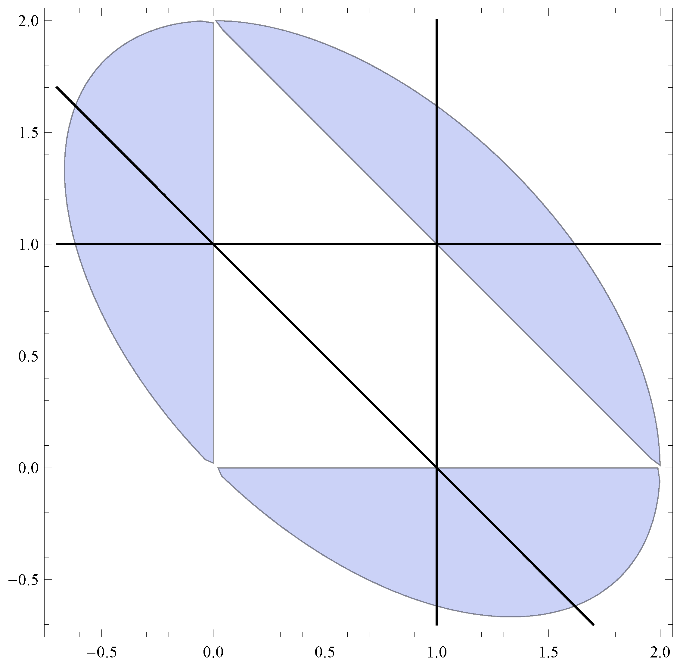
of some upwards skip-free Lévy chain, which can jump down by at most (and does jump down by) l units (this imposes some set of algebraic restrictions on the elements of $\{{\lambda }_1,\dots ,{\lambda }_{l+1}\}$). A priori one then has access to the zeros of the characteristic polynomial, and it remains to use the linear recursion in order to determine the first $l+1$ values of W, thereby finding (via solving a set of linear equations of dimension $l+1$) the sought-after particular solution of (20) (with $q=0$), that is W. A particular parameter set for the zeros is depicted in Figure 1 and the following is a concrete example of this procedure.

• “Reverse-engineered” chain. Let $l=2$, $p=\frac{1}{2}$ and, with reference to (the caption of) Figure 1, ${\lambda }_1=1$, ${\lambda }_2=-\frac{1}{2}$, ${\lambda }_3=\frac{3}{2}$. Then this corresponds (in the sense that has been made precise above) to an upwards skip-free Lévy chain with $\lambda /\lambda \left(\mathbb{R}\right)=\frac{1}{2}{\delta }_1+\frac{1}{8}{\delta }_{-1}+\frac{3}{8}{\delta }_{-2}$ and with $W\left(n\right)=A+B{(-\frac{1}{2})}^n+C{\left(\frac{3}{2}\right)}^n$, for all $n\in {\mathbb{Z}}_{+}$, for some $\{A,B,C\}\subset \mathbb{R}$. Choosing (say) $\lambda \left(\mathbb{R}\right)=2$, we have from Proposition 4, $W\left(0\right)=1$; and then from (20), $W\left(1\right)=2$, $W\left(2\right)=\frac{15}{4}$. This renders $A=-\frac{4}{3}$, $B=\frac{1}{12}$, $C=\frac{9}{4}$.

An example in which the support of $\lambda$ is not bounded, but one can still obtain closed form expressions in terms of elementary functions, is the following.

• “Geometric” chain. Assume $p\in (0,1)$, take an $a\in (0,1)$, and let $q_l=(1-p)(1-a)a^{l-1}$ for $l\in \mathbb{N}$. Then (20) implies for $z\left(k\right):=W\left(k\right)/a^k$ that $paz(k+1)=z\left(k\right)-{\sum }_{l=1}^k(1-p)(1-a)z(k-l)/a$, i.e., for $\gamma \left(k\right):={\sum }_{l=0}^{k}z\left(l\right)$ the relation $p{a}^2\gamma (k+1)-(a+p{a}^2)\gamma \left(k\right)+(1-p+pa)\gamma (k-1)=0$, a homogeneous second order linear difference equation with constant coefficients. Specialize now to $p=a=\frac{1}{2}$ and take $\gamma =\lambda \left(\mathbb{R}\right)=2$. Solving the difference equation with the initial conditions that are got from the known values of $W\left(0\right)$ and $W\left(1\right)$ leads to $W\left(k\right)=2{\left(\frac{3}{2}\right)}^k-1$, $k\in {\mathbb{Z}}_{+}$. This example is further developed in Section 5, in the context of the modeling of the capital surplus process of an insurance company.

Beyond this “geometric” case it seems difficult to come up with other Lévy measures for X that have unbounded support and for which W could be rendered explicit in terms of elementary functions.

We close this section with the following remark and corollary (cf. (Biffis and Kyprianou 2010, eq. (12)) and (Avram et al. 2004, Remark 5), respectively, for their spectrally negative analogues): for them we no longer assume that $h=1$.

Remark 8.

Let L be the infinitesimal generator (Sato 1999, p. 208, Theorem 31.5) of X. It is seen from (22), that for each $q\ge 0$, $\left((L-q)W^{\left(q\right)}\right){{|}_{{\mathbb{R}}_{+}}=\left((L-q)Z^{\left(q\right)}\right)|}_{{\mathbb{R}}_{+}}=0$.

Corollary 2.

For each $q\ge 0$, the stopped processes Y and Z, defined by $Y_t:=e^{-q(t\wedge T_0^{-})}{W}^{\left(q\right)}\circ X_{t\wedge T_0^{-}}$ and $Z_t:=e^{-q(t\wedge T_0^{-})}{W}^{\left(q\right)}\circ X_{t\wedge T_0^{-}}$, $t\ge 0$, are nonnegative $\mathsf{P}$-martingales with respect to the natural filtration ${\mathbb{F}}^X={\left({\mathcal{F}}_s^X\right)}_{s\ge 0}$ of X.

Proof. 

We argue for the case of the process Y, the justification for Z being similar. Let ${\left(H_k\right)}_{k\ge 1}$, $H_0:=0$, be the sequence of jump times of X (where, possibly by discarding a $\mathsf{P}$-negligible set, we may insist on all of the $T_k$, $k\in {\mathbb{N}}_0$, being finite and increasing to $+\infty$ as $k\to \infty$). Let $0\le s<t$, $A\in {\mathcal{F}}_s^X$. By the MCT it will be sufficient to establish for $\{l,k\}\subset {\mathbb{N}}_0$, $l\le k$, that:

$$\mathsf{E}[𝟙(H_l\le s<H_{l+1}){𝟙}_A{Y}_t𝟙(H_k\le t<H_{k+1})]=\mathsf{E}[𝟙(H_l\le s<H_{l+1}){𝟙}_A{Y}_s𝟙(H_k\le t<H_{k+1})].$$

(25)

On the left-hand (respectively right-hand) side of (25) we may now replace $Y_t$ (respectively $Y_s$) by $Y_{H_k}$ (respectively $Y_{H_l}$) and then harmlessly insist on $l<k$. Moreover, up to a completion, ${\mathcal{F}}_s^X\subset \sigma \left({(H_m\wedge s,X(H_m\wedge s))}_{m\ge 0}\right)$. Therefore, by a $\pi$/$\lambda$-argument, we need only verify (25) for sets A of the form: $A={\bigcap }_{m=1}^M\{H_m\wedge s\in A_m\}\cap \{X(H_m\wedge s)\in B_m\}$, $A_m$, $B_m$ Borel subsets of $\mathbb{R}$, $1\le m\le M$, $M\in \mathbb{N}$. Due to the presence of the indicator $𝟙(H_l\le s<H_{l+1})$, we may also take, without loss of generality, $M=l$ and hence $A\in {\mathcal{F}}_{H_l}^X$. Furthermore, $\mathcal{H}:=\sigma (H_{l+1}-H_l,H_k-H_l,H_{k+1}-H_l)$ is independent of ${\mathcal{F}}_{H_l}^X\vee \sigma \left(Y_{H_k}\right)$ and then $\mathsf{E}[Y_{H_k}|{\mathcal{F}}_{H_l}^X\vee \mathcal{H}]=\mathsf{E}[Y_{H_k}|{\mathcal{F}}_{H_l}^X]=Y_{H_l}$, $\mathsf{P}$-a.s. (as follows at once from (22) of Proposition 9), whence (25) obtains. ☐

5. Application to the Modeling of an Insurance Company’s Risk Process

Consider an insurance company receiving a steady but temporally somewhat uncertain stream of premia—the uncertainty stemming from fluctuations in the number of insurees and/or simply from the randomness of the times at which the premia are paid in—and which, independently, incurs random claims. For simplicity assume all the collected premia are of the same size $h>0$ and that the claims incurred and the initial capital $x\ge 0$ are all multiples of h. A possible, if somewhat simplistic, model for the aggregate capital process of such a company, net of initial capital, is then precisely the upwards skip-free Lévy chain X of Definition 1.

Fix now the X. We retain the notation of the previous sections, and in particular of Section 4.4, assuming still that $h=1$ (of course this just means that we are expressing all monetary sums in the unit of the sizes of the received premia).

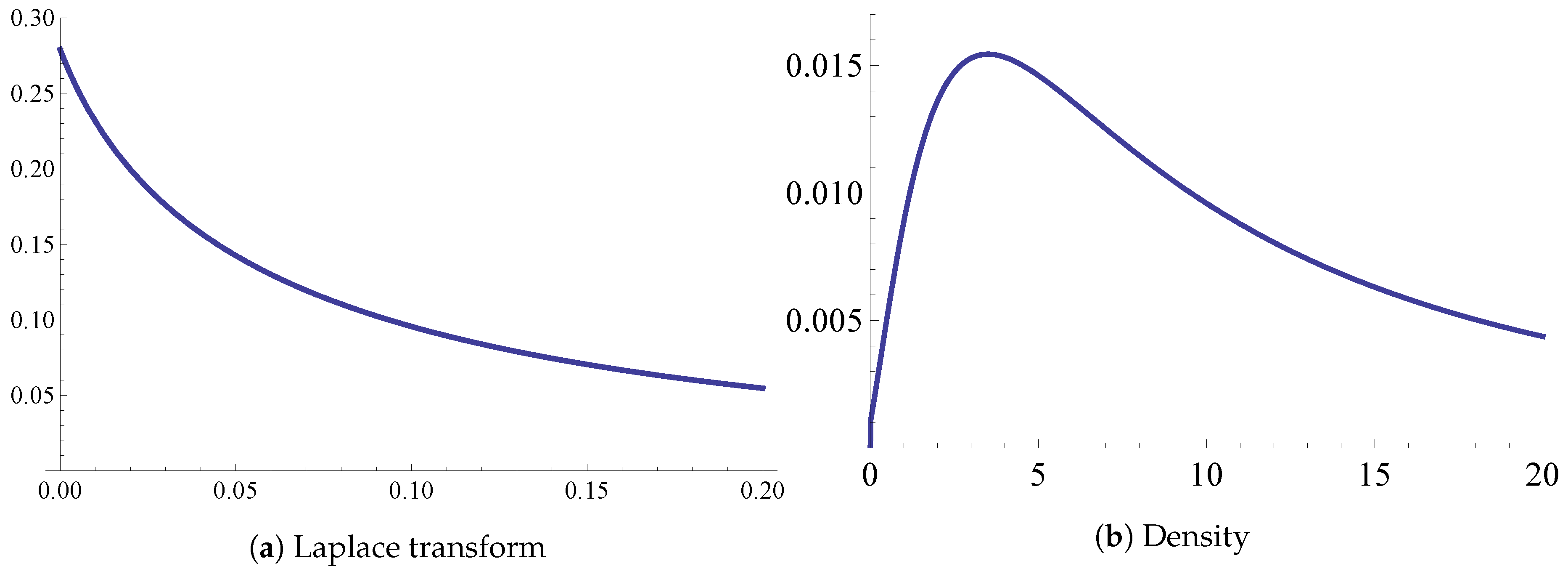
As an illustration we may then consider the computation of the Laplace transform (and hence, by inversion, of the density) of the time until ruin of the insurance company, which is to say of the time $T_x^{-}$.

To make it concrete let us take the parameters as follows. The masses of the Lévy measure on the down jumps: $\lambda \left(\{-k\}\right)={\left(\frac{1}{2}\right)}^k$, $k\in \mathbb{N}$; mass of Lévy measure on the up jump: $\lambda \left(\left\{1\right\}\right)=\frac{1}{2}+{\sum }_{n=1}^{\infty }n·{\left(\frac{1}{2}\right)}^n=\frac{5}{2}$ /positive “safety loading” $s:=\frac{1}{2}$/; initial capital: $x=10$. This is a special case of the “geometric” chain from Section 4.4 with $\gamma =\frac{7}{2}$, $p=\frac{5}{7}$ and $a=\frac{1}{2}$ (see p. 20 for a). Setting, for $k\in {\mathbb{N}}_0$, ${\gamma }^{\left(q\right)}\left(k\right):={\sum }_{l=0}^k{W}^{\left(q\right)}\left(l\right)2^l$ produces the following difference equation: $5{\gamma }^{\left(q\right)}(k+1)-(19+4q){\gamma }^{\left(q\right)}\left(k\right)+(18+4q){\gamma }^{\left(q\right)}(k-1)=0$, $k\in \mathbb{N}$. The initial conditions are ${\gamma }^{\left(q\right)}\left(0\right)=W^{\left(q\right)}\left(0\right)=\frac{2}{5}$ and ${\gamma }^{\left(q\right)}\left(1\right)={\gamma }^{\left(q\right)}\left(0\right)+2W^{\left(q\right)}\left(1\right)=\frac{2}{5}+{\left(\frac{2}{5}\right)}^2(7+2q)$. Finishing the tedious computation with the help of Mathematica produces the results reported in Figure 2.

On a final note, we should point out that the assumptions made above concerning the risk process are, strictly speaking, unrealistic. Indeed (i) the collected premia will typically not all be of the same size, and, moreover, (ii) the initial capital, and incurred claims will not be a multiple thereof. Besides, there is no reason to believe (iii) that the times that elapse between the accrual of premia are (approximately) i.id. exponentially distributed. Nevertheless, these objections can be reasonably addressed to some extent. For (ii) one just need to choose h small enough so that the error committed in “rounding off” the initial capital and the claims is negligible (of course even a priori the monetary units are not infinitely divisible, but e.g., $h=0.01€$, may not be the most computationally efficient unit to consider in this context). Concerning (i) and (iii) we would typically prefer to see a premium drift (with slight stochastic deviations). This can be achieved by taking $\lambda \left(\right\{h\left\}\right)$ sufficiently large: we will then be witnessing the arrival of premia with very high-intensity, which by the law of large numbers on a large enough time scale will look essentially like premium drift (but slightly stochastic), interdispersed with the arrivals of claims. This is basically an approximation of the Cramér-Lundberg model in the spirit of Mijatović et al. (2015), which however (because we are not ultimately effecting the limits $h\downarrow 0$, $\lambda \left(\right\{h\left\}\right)\to \infty$) retains some stochasticity in the premia. Keeping this in mind, it would be interesting to see how the upwards skip-free model behaves when fitted against real data, but this investigation lies beyond the intended scope of the present text.

References

- Asmussen, Søren, and Hansjörg Albrecher. 2010. Ruin Probabilities. Advanced series on statistical science and applied probability; Singapore: World Scientific. [Google Scholar]
- Avram, Florin, Andreas E. Kyprianou, and Martijn R. Pistorius. 2004. Exit Problems for Spectrally Negative Lévy Processes and Applications to (Canadized) Russian Options. The Annals of Applied Probability 14: 215–38. [Google Scholar]
- Avram, Florin, Zbigniew Palmowski, and Martijn R. Pistorius. 2007. On the optimal dividend problem for a spectrally negative Lévy process. The Annals of Applied Probability 17: 156–80. [Google Scholar] [CrossRef]
- Avram, Florin, and Matija Vidmar. 2017. First passage problems for upwards skip-free random walks via the Φ, W, Z paradigm. arXiv, arXiv:1708.0608. [Google Scholar]
- Bao, Zhenhua, and He Liu. 2012. The compound binomial risk model with delayed claims and random income. Mathematical and Computer Modelling 55: 1315–23. [Google Scholar] [CrossRef]
- Bertoin, Jean. 1996. Lévy Processes. Cambridge Tracts in Mathematics. Cambridge: Cambridge University Press. [Google Scholar]
- Bhattacharya, Rabindra Nath, and Edward C. Waymire. 2007. A Basic Course in Probability Theory. New York: Springer. [Google Scholar]
- Biffis, Enrico, and Andreas E. Kyprianou. 2010. A note on scale functions and the time value of ruin for Lévy insurance risk processes. Insurance: Mathematics and Economics 46: 85–91. [Google Scholar]
- Bingham, Nicholas Hugh, Charles M. Goldie, and Jozef L. Teugels. 1987. Regular Variation. Encyclopedia of Mathematics and its Applications. Cambridge: Cambridge University Press. [Google Scholar]
- Brown, Mark, Erol A. Peköz, and Sheldon M. Ross. 2010. Some results for skip-free random walk. Probability in the Engineering and Informational Sciences 24: 491–507. [Google Scholar] [CrossRef]
- Bühlmann, Hans. 1970. Mathematical Methods in Risk Theory. Grundlehren der mathematischen Wissenschaft: A series of comprehensive studies in mathematics; Berlin/ Heidelberg: Springer. [Google Scholar]
- Chiu, Sung Nok, and Chuancun Yin. 2005. Passage times for a spectrally negative Lévy process with applications to risk theory. Bernoulli 11: 511–22. [Google Scholar] [CrossRef]
- De Vylder, Florian, and Marc J. Goovaerts. 1988. Recursive calculation of finite-time ruin probabilities. Insurance: Mathematics and Economics 7: 1–7. [Google Scholar] [CrossRef]
- Dickson, David C. M., and Howard R. Waters. 1991. Recursive calculation of survival probabilities. ASTIN Bulletin 21: 199–221. [Google Scholar] [CrossRef]
- Doney, Ronald A. 2007. Fluctuation Theory for Lévy Processes: Ecole d’Eté de Probabilités de Saint-Flour XXXV-2005. Edited by Jean Picard. Number 1897 in Ecole d’Eté de Probabilités de Saint-Flour. Berlin/Heidelberg: Springer. [Google Scholar]
- Engelberg, Shlomo. 2005. A Mathematical Introduction to Control Theory. Series in Electrical and Computer Engineering; London: Imperial College Press, vol. 2. [Google Scholar]
- Hubalek, Friedrich, and Andreas E. Kyprianou. 2011. Old and New Examples of Scale Functions for Spectrally Negative Lévy Processes. In Seminar on Stochastic Analysis, Random Fields and Applications VI. Edited by Robert Dalang, Marco Dozzi and Francesco Russo. Basel: Springer, pp. 119–45. [Google Scholar]
- Kallenberg, Olav. 1997. Foundations of Modern Probability. Probability and Its Applications. New York and Berlin/Heidelberg: Springer. [Google Scholar]
- Karatzas, Ioannis, and Steven E. Shreve. 1988. Brownian Motion and Stochastic Calculus. Graduate Texts in Mathematics. New York: Springer. [Google Scholar]
- Kyprianou, Andreas E. 2006. Introductory Lectures on Fluctuations of Lévy Processes with Applications. Berlin/ Heidelberg: Springer. [Google Scholar]
- Marchal, Philippe. 2001. A Combinatorial Approach to the Two-Sided Exit Problem for Left-Continuous Random Walks. Combinatorics, Probability and Computing 10: 251–66. [Google Scholar] [CrossRef]
- Mijatović, Aleksandar, Matija Vidmar, and Saul Jacka. 2014. Markov chain approximations for transition densities of Lévy processes. Electronic Journal of Probability 19: 1–37. [Google Scholar] [CrossRef]
- Mijatović, Aleksandar, Matija Vidmar, and Saul Jacka. 2015. Markov chain approximations to scale functions of Lévy processes. Stochastic Processes and their Applications 125: 3932–57. [Google Scholar] [CrossRef]
- Norris, James R. 1997. Markov Chains. Cambridge series in statistical and probabilistic mathematics; Cambridge: Cambridge University Press. [Google Scholar]
- Parthasarathy, Kalyanapuram Rangachari. 1967. Probability Measures on Metric Spaces. New York and London: Academic Press. [Google Scholar]
- Quine, Malcolm P. 2004. On the escape probability for a left or right continuous random walk. Annals of Combinatorics 8: 221–23. [Google Scholar] [CrossRef]
- Revuz, Daniel, and Marc Yor. 1999. Continuous Martingales and Brownian Motion. Berlin/Heidelberg: Springer. [Google Scholar]
- Rudin, Walter. 1970. Real and Complex Analysis. International student edition. Maidenhead: McGraw-Hill. [Google Scholar]
- Sato, Ken-iti. 1999. Lévy Processes and Infinitely Divisible Distributions. Cambridge studies in advanced mathematics. Cambridge: Cambridge University Press. [Google Scholar]
- Spitzer, Frank. 2001. Principles of Random Walk. Graduate texts in mathematics. New York: Springer. [Google Scholar]
- Vidmar, Matija. 2015. Non-random overshoots of Lévy processes. Markov Processes and Related Fields 21: 39–56. [Google Scholar]
- Wat, Kam Pui, Kam Chuen Yuen, Wai Keung Li, and Xueyuan Wu. 2018. On the compound binomial risk model with delayed claims and randomized dividends. Risks 6: 6. [Google Scholar] [CrossRef]
- Xiao, Yuntao, and Junyi Guo. 2007. The compound binomial risk model with time-correlated claims. Insurance: Mathematics and Economics 41: 124–33. [Google Scholar] [CrossRef]
- Yang, Hailiang, and Lianzeng Zhang. 2001. Spectrally negative Lévy processes with applications in risk theory. Advances in Applied Probability 33: 281–91. [Google Scholar] [CrossRef]