Can Pension Funds Partially Manage Longevity Risk by Investing in a Longevity Megafund?


1
ISFA, Laboratoire SAF EA2429, Univ Lyon—Université Claude Bernard Lyon 1, F-69366 Lyon, France
2
Prim’Act, 42 Avenue de la Grande Armée, 75017 Paris, France
*
Author to whom correspondence should be addressed.
†
These authors are researcher at SAF laboratory (EA n°2429). Frédéric Planchet is also consulting actuary at Prim’Act.
Risks 2018, 6(3), 67; https://doi.org/10.3390/risks6030067
Submission received: 19 March 2018
/
Revised: 14 June 2018
/
Accepted: 22 June 2018
/
Published: 2 July 2018
(This article belongs to the Special Issue New Perspectives in Actuarial Risk Management)
Abstract
:Pension funds, which manage the financing of a large share of global retirement schemes, need to invest their assets in a diversified manner and over long durations while managing interest rate and longevity risks. In recent years, a new type of investment has emerged, that we call a longevity megafund, which invests in clinical trials for solutions against lifespan-limiting diseases and provides returns positively correlated with longevity. After describing ongoing biomedical developments against ageing-related diseases, we model the needed capital for pension funds to face longevity risk and find that it is far above current practices. After investigating the financial returns of pharmaceutical developments, we estimate the returns of a longevity megafund. Combined, our models indicate that investing in a longevity megafund is an appropriate method to significantly reduce longevity risk and the associated economic capital need.
Keywords:
longevity; mortality; longevity risk; pension fund; megafund; biomedical; biology of aging; pharma; model; needed capital1. Introduction
In 2012, Fernandez et al. (2012) presented the concept of “cancer megafund”, a financial solution to stimulate the financing of potential solutions to cancer. It is an alternative to the current pharmaceutical development model where dramatic decreases in profitability are described (see Scannell et al. 2012) that make investors reluctant to bet on biomedical innovation. In essence, the concept is about risk mutualization: the expected rate of return of 150 diverse and carefully selected biomedical drug developments is similar to that of a few carefully selected developments but, owing to the law of large numbers, the risk is considerably smaller. Since investing in many developments requires many investors, the megafund concept includes securitization techniques to attract enough investors, notably pension funds and insurance companies. The fund is split between two financial instruments: “Research Backed Obligations” (RBOs), which provide investors with fixed returns, backed by clinical trials, and equity, which captures the remaining profits.
The concept is rapidly proposed for other applications than cancer, such as Alzheimer’s disease (see Lo et al. 2014), orphan diseases (see Fagnan et al. 2014), and general biomedical innovation in large, in London, the USA, Australia, or Sweden (see Swedish Agency for Growth Policy Analysis 2017). In parallel, Boissel (2013), Marko (2013), Tenenbaum (2013), Fagnan et al. (2014, 2015), Lo and Naraharisetti (2014), Lo (2015), Yang et al. (2016), and Hull (2016) underline both the broad potential applications and risks of the megafund structure. Essentially, in order to finance many “long shots”, whether health-related or not, the projects should be largely uncorrelated as opposed to all focused on the same disease or set of diseases. There are additional considerations to take into account for a megafund to mitigate risk: according to Hull (2016) and Yang et al. (2016), each individual project should have a minimum probability of success; according to Yang et al. (2016), the megafund should not be structured in too many financial components to align investors’ interests.
In 2014, the concept emerges that targeting various diseases has an additional desirable effect than a better diversification: as described by Stein (2016) and MacMinn and Zhu (2017), it can hedge longevity risk, i.e., the financial loss if people live longer than planned. They suggest that “biomedical RBOs” can hedge longevity risk. The link would not be perfect. For example, some life-extending drugs may be developed in which the megafund has not invested. Still, it would provide a better longevity hedge than alternative longevity-linked securities (see MacMinn and Zhu 2017). This is unexpected good news as Pension funds and insurance companies are essential stakeholders for a megafund to reach its critical mass. This becomes even better news as Pension funds and insurance companies are not prone to finance treatments that lead to longer pensions to be paid.
Given such impressive conclusions that a megafund could both support medical discoveries and the financing of pensions, this paper gets back to basics and checks some foundations for such an interest in pension funds to invest in a longevity megafund. The analysis of fine hedging adjustments, as in MacMinn and Zhu (2017), is beyond the scope of this article. Instead, we investigate more fundamental aspects of the equation that were partly ignored, such as the magnitude of longevity risk and the magnitude of rates of returns. Focusing on the link with longevity risk, we name the structure “longevity megafund” rather than “biomedical megafund” when it invests into solutions to life-threatening diseases rather than all kinds of diseases.
The paper is organized in three main sections. In Section 2, and with greater details in Appendix A, we model the potential size of longevity risk. We conclude that the necessary prudential capital to cover longevity risk is significantly higher than what is common practice in the industry today. In Section 3, and with greater details in Appendix B, we model the expected rate of return of a biomedical megafund and a longevity megafund. We attempt to quantify key factors in the equation such as the cost and success rate of clinical trials, the profitability of pharmaceutical developments, both under the current longevity trend and with scenarios of increasing human longevity. In Section 4, we cross both longevity risk and rate of return to assess the attractiveness of a longevity megafund to pension fund asset managers. We then conclude and discuss some remaining aspects that we could not study here.
In order to ease the understanding, Appendix C at the very end of the article lists figures, tables, and variables by theme: “Longevity model”, “Returns of pharmaceutical developments”, and “Pension fund needed capital”.
2. Potential Size of Longevity Risk
Stein (2016) and MacMinn and Zhu (2017) highlighted that pension funds may be interested in investing in a longevity megafund to manage some of their longevity risk. Longevity risk is generally directly or indirectly estimated by how well models match historical mortality data. However, as described by Debonneuil et al. (2017), not only do frequent actuarial models unknowingly project decelerating life expectancy trends, advances on the largest source of longevity risk are largely ignored: a likely forthcoming wave of biomedical solutions to old age conditions that comes from biology of aging and animal models. Here, we therefore aim to take into account such advances, and we suggest a simple model that does not produce decelerating life expectancy trends to generate longevity scenarios. We then use a model of a pension fund to estimate the needed prudential capital with respect to longevity risk.
2.1. Solutions Derived from Biology of Aging Are Reaching Clinics
In the 19th and 20th centuries, infant mortality rates and young adult mortality rates have dropped so that the future trend of life expectancy is now to a large extent a matter of solutions to old age conditions (see Vallin and Meslé 2010 and Debonneuil et al. 2011).
In the beginning of the 21st century, a series of biomedical discoveries suggest that mortality rates may drop at old age as well. The series started with animal models of human aging and is now turning to humans. In 2008, Ayyadevara et al. (2008) were able to extend the lifespan of laboratory nematodes by circa ten times with one single gene change and Bartke et al. (2008) were able to extend the lifespan of laboratory mice by 70% with a combination of gene change and diet. Since then, a vast range of successful methods in animals were reproduced at the level of cells and tissues in humans and human trials are now being discussed (see Barardo et al. 2017 and Moskalev et al. 2017). The translatability to humans is supported by several discoveries. In particular, some mutations that increase the lifespans of rodents are seen in long-lived human families (see Kenyon 2010). Also, low-caloric diets, that can extend the approximate 2-year lifespan of rodents by more than 40%, extend the approximate 6-year lifespan of primates by more than 50% (see Pifferi et al. 2018), without observed sign of physical nor mental health deterioration. The graft of bio-printed organs (see Ravnic et al. 2017; and Mir and Nakamura 2017) and the in vivo degradation of old tissues that the body then naturally replaces by younger tissue (see Fahy 2003; Ocampo et al. 2016; Mosteiro et al. 2016; and Mendelsohn et al. 2017) are already being tested in specific clinical settings. The latter advances show that science is not only on its way to slow down human aging but also to restore youthful characteristics to the body once old.
One may then expect much better health at old ages, which in turn means lower mortality rates and longer lives. By how much? The life expectancy impact of curing diseases is inconsistently estimated because beyond each disease itself there is a largely unknown associated global burden on the body (see Martin et al. 2003; Arias et al. 2013; and Guibert et al. 2017). Where models or parameters are to be chosen, psychological ceilings lead to underestimate parameters. This is how in 1928 Dublin (1928) predicted an ultimate average life expectancy limit of 64.75 and how in 1990 Olshansky et al. (1990) increased that estimate to 85, which is already less than the woman life expectancy in Japan.
Keeping maximum human lifespan around the age of 115 is one of those arbitrary ceilings. It seems to be such lately and this leads for example Vig and Le Bourg (2017) to consider that it will necessarily remain as such. But the latter is not a proof, as noted by Gavrilov et al. (2017) who even observes a constant centenarian mortality since 1940. Comparing the effects of current interventions in various animal species and humans Ben-Haim et al. (2017) suggests a further increase of 30% of lifespan, i.e., 150 years of maximal lifespan may be at reasonable reach based on ongoing developments.
Until a few years ago, the field of biology of aging was only about fundamental research and largely away from pharmaceutical developments. The pharmaceutical industry used to apply methods developed for single, acute diseases to multiple, chronic diseases (see Thiem et al. 2011; Roman and Ruiz-Cantero 2017) instead of targeting the underlying aging and regenerative processes as described above. Since about 2015, various biotech companies have raised funds to bring biology of aging results to the clinics (see De Magalhães et al. 2017; and Debonneuil et al. 2017). Various investor reports, books, and conferences consider that current retired persons may be the first populations to benefit from such advances (see Mellon and Chalabi 2017; Pratt 2016; and Casquillas 2016). When essentially focusing on hair and skin aging, which were the main anti-aging industry drivers until recently, estimated sizes of the anti-aging market are $122 Bn in 2013, 140 in 2015, 192 in 2019, and 217 in 2021 (see Zion Market Research 2017; Transparency Market Research 2014) which explains why the financial industry is starting to drive this move.
Of course, these advances may also require non-negligible adjustments in retirement systems: retirement systems face the “longevity risk” that retirements must be paid longer than financially planned. Current retirement systems essentially stem from the middle of the 20th century, when most young workers were not expected to reach retirement age, and they depend on various mortality tables that are regularly updated but that empirically under-estimate historical life expectancy trends (see Antolin and Mosher 2014; and Debonneuil et al. 2017). In the USA only, if deaths caused by cardiovascular diseases and cancer were eliminated, the fiscal imbalance of Social Security and Medicare programs may be as high as $87 trillion in present value (see Zhavoronkov et al. 2012).
2.2. Model of Longevity Risk
We choose a model, derived from Bongaarts (2005) and Debonneuil et al. (2017), that is simple enough to be traceable and understandable but incorporates key features that are rarely encountered in actuarial sciences: as we will see, it generates non-decelerating life expectancies and is relatively universal owing to its simplicity. It is defined by this logistic formula for the annual mortality rate of someone aged x in t years:
where t = 0 corresponds to 1 January 2020, as explained in Appendix A, φ represents the annual increase of life expectancy at birth, for t < 0 it is set to the current φ = 20% trend and for t ≥ 0 it is randomly selected based on a probability density function to describe various possibilities in the future:
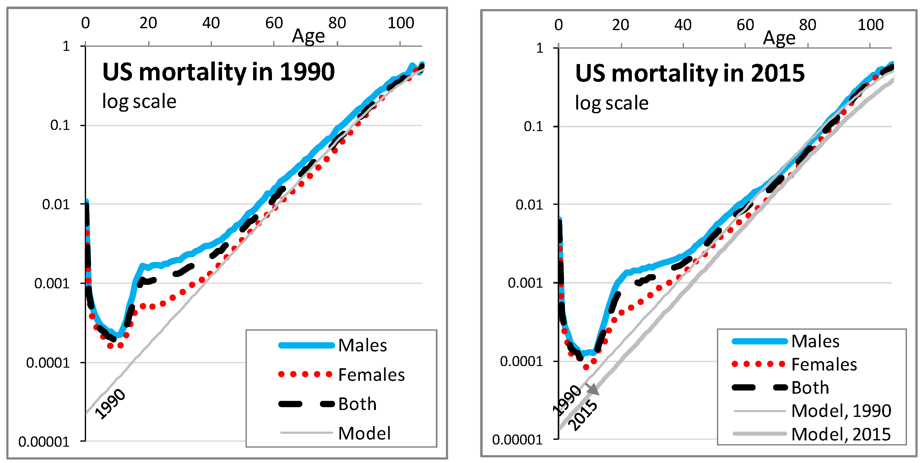
Appendix A describes in greater details the reasons for choosing this model and how the parameters are calibrated (a = 11.3, b = 10%, φ up to t = 0 then s = 1 to draw a random φ). It notably defines remaining life expectancy at age x and time t, , that is used for the calibration. Overall, the model and its parameters are chosen to fit mortality rates and life expectancy in Japan, as indicated in Figure 1, as a representation of the life expectancy of pensioners weighted by amount (that are higher than the general population as higher amounts are correlated with lower mortality due to social inequalities). The longevity level at time t = 0, a, can of course be adjusted to model specific populations of pensioners, but what mostly matters for what follows is the range of possible longevity trends for t > 0.
2.3. Implication for a Pension Fund in Terms of Needed Prudential Capital
Let us use a simple model of a pension fund to apply the longevity model and compute capital needs.
Population studied. We consider the following cohort defined as such at time t = 0: 300 employees of age 20, employees of age 21, employees of age 22, etc. until an age 64 and no retired persons. This provides a distribution of the population across ages that is roughly natural. When applying the mortality model, this corresponds to 13,000 people at time t = 0 (year 2020). We follow this closed portfolio over time (t = 1, 2, etc.) and every year people die according to mortality rates. For the sake of simplicity, we do not model arrivals nor departures. The number of people aged x at time t is then:
The formula is valid for workers aged 20 to 64 at t = 0, i.e., for t ≥ 0 and x < 65 + t and x ≥ 20 + t. Otherwise, this is not the cohort, so = 0. Summing over ages, numerically at t = 0 the cohort is composed of 13,295 employees.
Contributions and investments. Using Asset Liability Management (ALM) practice standards, we consider employees of different age tranches, each with different salaries per tranche, a contribution of 10%, and different returns per tranche, as shown in Table 1.
The increasing contributions of persons aged 20–34, 35–49, and 50–64 that are invested in decreasing degrees of risk. This is based on practice where younger people invest in more risky and potentially more profitable assets, whereas older people invest in safer assets with less profitability. For each of the three funds, dedicated to an age tranche, the annual return rate (i1, i2, i3) is normally distributed, which corresponds to a lognormal distribution of wealth. The volatilities are chosen with a Sharpe ratio of 1 (personal experience with such a level), a risk-free rate of 1% and a 2-by-2 correlation of 50%1 between the three fund return rates:
We consider that in the past, the annual returns were exactly 5%, 4%, and 2% (depending on the age tranche). In order to avoid modeling complex contractual clauses we consider that the accumulated capital of a worker who dies serves as accumulated capital for the group of persons aged x at t (no removal of capital).
Under such assumptions, at t = 0:
We also have = 0 for x ≤ 20 (no contributions yet) and x ≥ 65 (at time 0 we only consider workers). Then, year after year between t − 1 and t,
where c and i are the contributions and annual investment returns as defined by Table 1 and Equations (4) and (5).
Initial wealth. By initial wealth we mean the total accumulated capital at t = 0:
Numerically, this leads to an initial wealth of approximately 2 Bn (1,995,578,577). In what follows, we will express the needed prudential capital by amount of initial wealth.
Benefits at retirement. Retirement benefits depend on the accumulated capital at age 65, that is here converted in a lifelong annuity by an insurer who is responsible for paying corresponding benefits throughout the life of the pensioners.
Instead of having to model interest rates and increases of annual benefits during retirement, we take the simplifying assumption that increases are such that the two compensate: the duration of benefit payments is then the remaining lifespans at age 65. If is the annual benefit paid to the workers who retire at time t, the present value of benefits at time t is then .
At time t, however, a longevity trend is not necessarily observed. We consider that the conversion from the accumulated capital to the benefit amount is done based on the mortality model with φ = 20%. Since actuarial tables generally have decelerating trends (see Debonneuil et al. 2017), insurers would consider it prudent compared to existing practices. If longevity increases much, the use of φ = 20% remains a plausible base since actuarial tables do not evolve immediately after observing overestimations of mortality rates (see Vaupel 2010).
In order to face risks, the insurer may convert only a part of , where is between 0 and 1. For the sake of simplicity, we consider = 1.
With that definition of benefit amounts, if the future longevity trend is φ = 20% then the mechanism in place to collect contributions and investment returns provide the right amount of money to pay all pensions. However, additional wealth is initially needed to face higher longevity trends.
Needed prudential capital. We define the needed prudential capital by the amount of money initially needed, in addition to initial wealth, to pay the pensions of the workers with a high probability.
In order to assess the needed prudential capital at t = 0 under the assumption of a given future scenario defined by the longevity trend and the investment returns (“”), we allow wealth to become negative (instead of claiming bankruptcy) and we measure wealth after all benefits were paid. is the present value of that final wealth, so that is the additional initial wealth that would have been needed to provide the right amount to pay retirement benefits in the future, without reaching bankruptcy. For the sake of simplicity, the discounting is performed along investments done, i.e., the wealth is divided by the value of an initial investment of 1 when invested in the different funds in the same proportion of contributions. In practice, long term investment choices and associated discounting may be optimized through the use of progressive utility (see El Karoui et al. 2014).
We generate 10,000 future scenarios of longevity trend and investment returns , using a Cholesky decomposition of the covariance matrix 〈〉 to simulate correlated returns. We compute 10,000 corresponding values of to compute the needed prudential capital, that we arguably define as being sufficient to pay retirement benefits in 90% of the simulated scenarios: a 90% VaR (Value at Risk).
This would mean that there is a 10% risk of not fully paying retirement benefits. The risk may be lower because adjustments may occur. For example, in case of difficulties, new business contributions would probably be used to some extent to pay the benefits of the older business. However, events can be worse than modeled and reactivity can be questioned with respect to retirement systems. In what follows, we will also compute the 85% VaR and 95% VaR as this choice has a material impact.
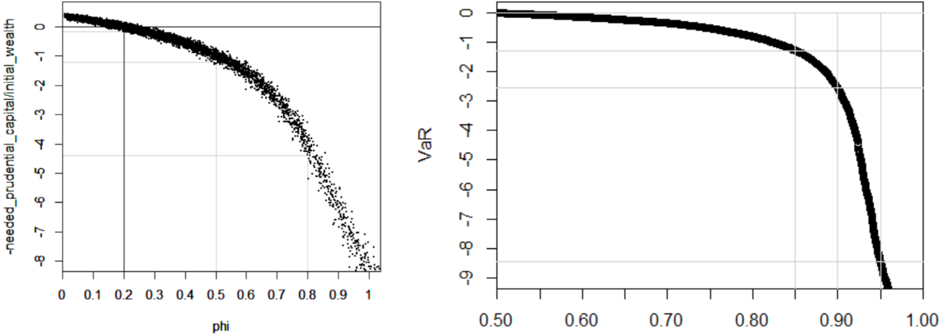
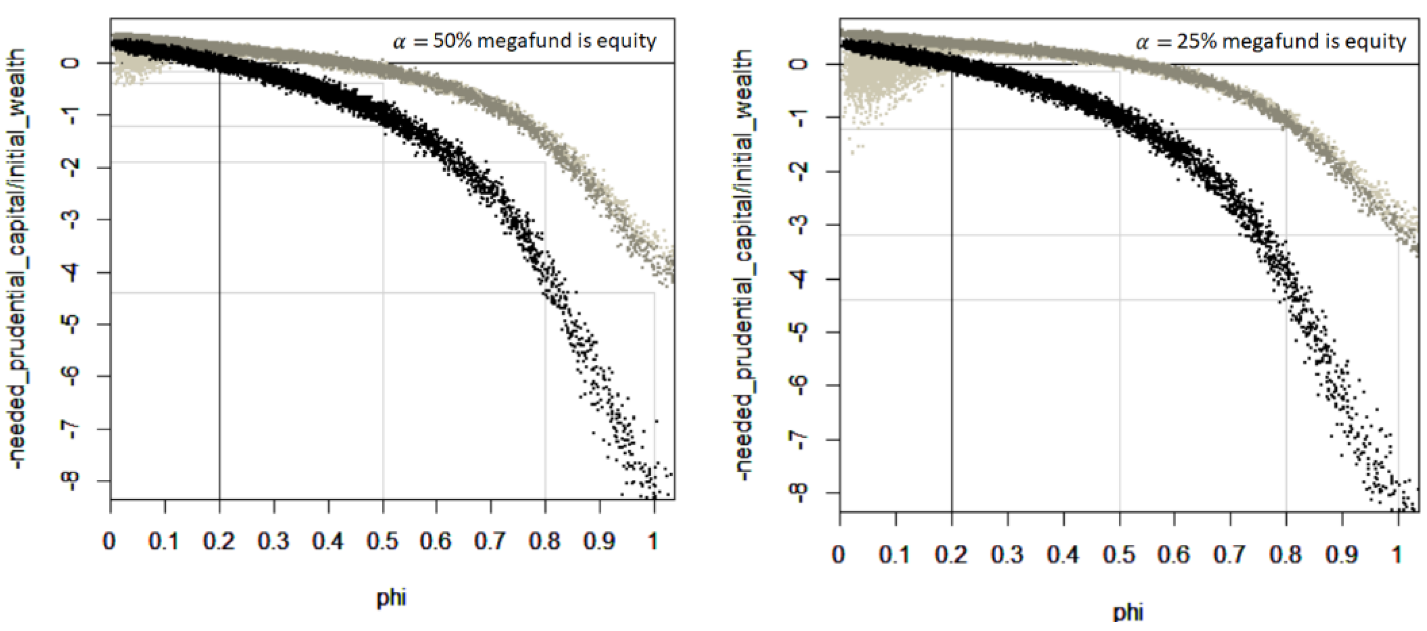
Results.Figure 2 shows the needed amount of additional initial wealth, expressed as a proportion of the initial wealth, depending on the future longevity trend.
If the current longevity trend continues ( = 20%) an additional capital of circa 15% of the initial wealth may be considered. This is due to the uncertainty of the fund returns—the thickness of the curve in Figure 2. Taking the average (the center of the black curve) instead of a VaR shows a perfectly neutral initial wealth.
However, if the longevity trend is the needed prudential capital should be slightly more than the initial wealth. If the longevity trend is , the needed prudential capital should be more than 4 times the initial wealth.
In practice, however, one does not know the future of longevity, so the prudential additional wealth shall cover a wide range of possible longevity trends. Using the lognormal distribution of longevity trends, our simulation suggests that the needed prudential capital is approximately 1.4 times, 2.7 times, or 8.4 times the initial wealth depending on whether a 85%, 90%, or 95% VaR is respectively considered. One might have expected that longevity risk is handled with a prudential capital of 10% or 30% of the initial wealth. This is not the case here because we consider the type of breakthroughs that were described at the beginning of the article and that are burgeoning. It is worth noting that in a Solvency II environment the solvency capital requirement is estimated with a short-term view of risks; here we consider the needed current capital with a long term view of risks given that pensions represent long term liabilities.
2.4. Conclusion of This Section
Longevity risk is not small, which could incentivize pension funds or other retirement payers to invest in the equity tranche of a longevity megafund provided it brings enough return, including enough return in a wide range of longevity scenarios.
3. Potential Rate of Return of a Longevity Megafund
In this section, we first discuss the rates of return of pharmaceutical developments, we then estimate their evolutions in case of longevity scenarios and we then investigate corresponding rates of return for the equity tranche of a longevity megafund.
3.1. Rate of Returns of Pharmaceutical Developments Today
There has been much debate on the rate of return of pharmaceutical developments. For example, the average research and development cost per pharmaceutical development has been reported to be $2558 M by DiMasi et al. (2016) but less than $59 M by Light and Warburton (2011). Appendix B navigates through such inconsistent historical reports, but also consistent open data and recent investigations, and concludes that the pharmaceutical development returns have been relatively stable. The return of a large portfolio of pharmaceutical developments can be put in a model defined by Fernandez et al. (2012) where an initial investment leads ten years later to a gain with a probability (success rate): the 10-year return is
and the annualized return is
Based on the analysis in Appendix B, the success rate from undertaking a first small clinical trial to commercial approval would typically be about 12%. The average research and development cost would typically be = $50 M, let us consider = $55 M or rather $60 M due to megafund management fees, and the average 10-year gain when selling results to pharmaceutical companies = $1.5 Bn. The corresponding annualized returns are then 11.6–12.5%. In fact, returns may be quite different depending on the strategy of the megafund, so the numbers initially chosen by Fernandez et al. (2012) for a cancer megafund seem reasonable to us for a longevity megafund under current conditions (i.e., the current longevity trend = 20%): = 3.1 and = 11.9%.
The next two sections investigate how megafund returns evolve with longevity trends, for a generic biomedical megafund and for a longevity megafund.
3.2. Evolution of Biomedical Megafund Returns with Longevity: “Linkage 1”
This section investigates how megafund returns evolve with longevity trends, for a generic biomedical megafund that invests in all kinds of pharmaceutical developments.
In the 19th and 20th centuries, infant mortality rates and young adult mortality rates have dropped. Now, the future of life expectancy will more and more become a matter of solutions to old age conditions (see Vallin and Meslé 2010). We apply that latter view in the context of how much successful pharmaceutical developments are paid when they extend lives.
Currently, biomedical developments and longevity are poorly linked: the approximate 3 months of increase in life expectancy per year are still largely a matter of improved lifestyles and many biomedical innovations address health needs that do not relate to longevity, for example, migraine or glaucoma treatments. The OECD estimates that 37.2% of the current longevity trend is due to health care spending, other factors being improved education, improved income, and decreased smoking and alcohol consumption (see OECD 2017). This means that biomedical innovation accounts for less than an additional month of life every year: out of approximately 35 new molecular entities and biologicals per year some may add one week but others zero days. Under such circumstances with longevity trends , the profitability of a biomedical megafund that invests in very diverse pharmaceutical developments, should be close to the one described above: and .
However, it is difficult to imagine that life expectancy may become much higher than the age of 100 only with lifestyle improvements (see Gavrilov et al. 2017): health care improvements will de facto be the main driver for large longevity increases. A longevity scenario is for example that 35 new molecular entities and biologicals are still produced per year but now they mostly address critical life limiting conditions, such that each therapy on average adds one week of year to life expectancy. Under that scenario, biomedical innovations alone increase life expectancy by 35 × 7/(365/12) = 8 months per year. The megafund gains would then depend on accepted costs per year of life saved through biomedical intervention.
Accepted costs notably increase with the perception of a critical need and with the ageing of populations (see Murphy and Topel 2006). An analysis in 1995 of 500 life-saving interventions suggested additional costs of $42 k per additional life-year but only $19 k for the specific case of medical interventions (see Tengs et al. 1995). However, for cancer patients this number was $54 k in 1995 and it ramped up to $217 k in 2013 (see Howard et al. 2015). In the UK the NICE used to accept biomedical innovation for 20 to 30k£ per additional healthy year of life (see Devlin 2003). Elsewhere, $50 k has long been the common reference and higher numbers are now often used (see Neumann et al. 2014). Based on all these numbers, we consider $50 k as a reasonable accepted cost per life year gain, and since pharmaceutical companies would typically pay 40% of the value to the megafund (Stewart et al. 2001) we consider that the gains provided by the megafund should be the order of $20 k per additional year of life per person (40% of $50 k).
Let us now design a model of megafund profitability that accounts for both low longevity scenarios and high longevity scenarios with some smooth intermediate shape. We use the following formula for the 10-year profitability :
where the coefficients, , and are defined as follows.
is a function of longevity that increases the profitability with longevity. Under strong longevity scenarios, the parameter is small compared to and then : represents the evolution of with longevity. Historically, this evolution can be estimated via the annual 35 new molecular entities and biologicals described above, that are taken by approximately 10 M patients in the years under patent:
with 11.4. The 10 M patient is an estimate provided by experts but it corresponds for example to 21% of 48.5 M of Americans over age 65 (see Human Mortality Database) which is half of those taking polypharmacy (see Kantor et al. 2015), a proxy for using one of the 35 drugs.
is a coefficient to set profitability at the right level. Historically, and so we take = to get for .
The residual performance of the megafund, due to factors not present in the equation, such as the quality of the fund managers, is a uniform random number between −1 and 1 given that the measure of = 10% is unsure by approximately 5% (see Thomas et al. 2016; Wong et al. 2018) and that prices are unsure too (as seen with the Royalty Pharma density above).
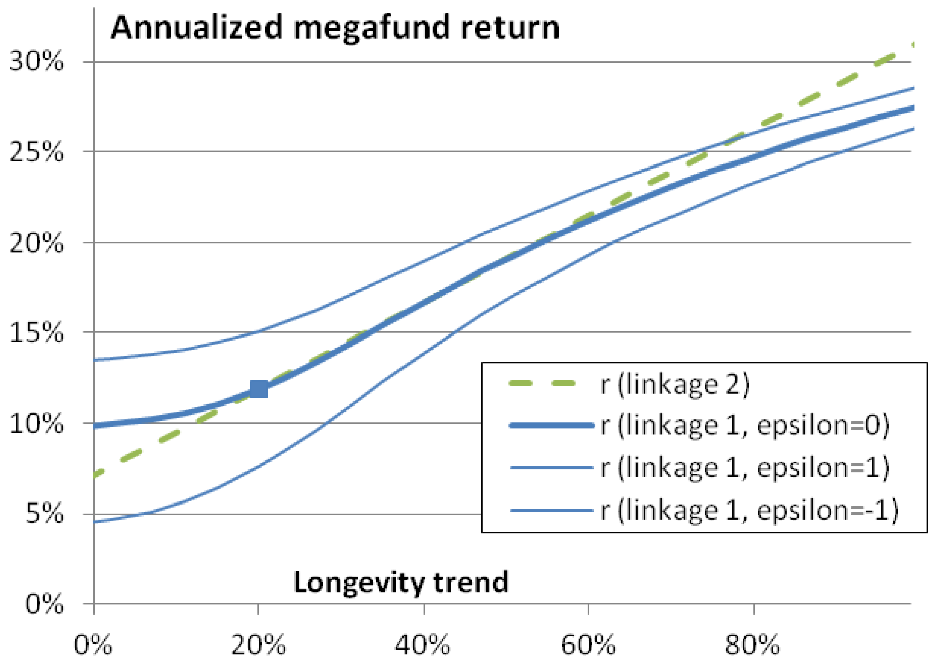
We call that link between longevity and returns “linkage 1”; it is for a megafund that invests in a large set of biomedical developments like the 35 new molecular entities and biologics mentioned above. Figure 3 shows the corresponding annualized profitability . With = 0, 1 and −1 the annual return under the current longevity trend is respectively 11.9%, 17%, and 7.6%. The curve is concave.
As we have seen, various assumptions have led to this link. This may lead to slightly higher or lower returns, which can be taken into account in definition. In practice, a megafund could have its own development strategy and have consequently greater or lower returns and document it for investors. In any case, as we will see, a pension fund could then adjust its share of investments in the megafund accordingly.
3.3. Evolution of Longevity Megafund Returns with Longevity: “Linkage 2”
This section investigates the link between megafund returns and longevity in case the megafund invests in solutions against aging processes and life-threatening diseases.
Various considerations could further strengthen or weaken the concavity of the curve observed in Figure 3. On the one hand, for example, the longevity wave may mostly occur via an improved success rate as many biology of aging discoveries may enter hospitals and offer various new ways to treat the aging and chronic diseases that are currently difficult to treat. On the other hand, as the accepted cost depends on the perceived criticality of needs (see Howard et al. 2015), it may be possible that new health treatments are not perceived as critical in a longevity scenario and the accepted cost may not necessarily increase.
Let us now consider a longevity megafund: a biomedical megafund that is particularly focusing on conditions that are linked with mortality and longevity. The return may be lower in case of low longevity trend and higher in case of high longevity trend, due to the returns provided by biology of aging solutions. Obviously and as we will see, this provides a better longevity risk management tool. Mathematically, the link between longevity and return would be less concave and we model it with a linear approximation of “linkage 1”:
This “linkage 2” is chosen to fit the approximately linear part of the “linkage 1” curve seen in Figure 3. With = 0, 1 and −1 the annual return under the current longevity trend is respectively 11.9%, 15.9%, and 7.9%.
3.4. Evolution of Megafund Equity Returns with Longevity
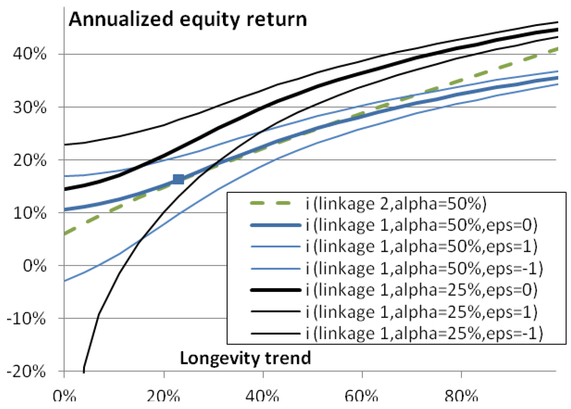
In practice, a pension fund may invest in the equity tranche of the megafund rather that in the whole megafund. A megafund must be structured into debt and equity (non-debt) because without the debt part, it would be difficult to find enough investors to have enough drug development programs financed for the megafund risk to become small compared to returns, hence to be financially attractive. The debt part, composed of “research-backed obligations” (RBOs), provides fixed annual returns: it cannot hedge longevity risk. Therefore, , the annualized return of the equity part of the megafund that provides gains in excess of RBOs, is the rate that matters to possibly cover longevity risk:
where is the equity percentage of investments in the megafund and where we supposed that the annual interest rate of the RBOs is . Indeed, if is the total of investments received by the megafund, is the investment in the equity tranche, is the gain generated 10 years, it first pays to the RBOs investors—who invested —and so that equity investors receive the reminder, : this must be compared to the initial investment 10 years earlier. When the 10-year return of drug development is , having or 25% of investments dedicated to the equity tranche leads to or , respectively: the equity share can be used as a lever to obtain higher returns if there are enough successful drug development programs (at the cost of reducing returns if there are not enough). Figure 4 shows the corresponding equity return as a function of longevity trend. Greater returns are found except with the stronger lever () and lowest longevity ( here): here, strongly negative returns are found, highlighting that the lever effect bears risks. Even though a pension fund should make gains when longevity is high, it should make sure these are sufficient in such a scenario.
4. In Which Cases Will a Pension Fund Benefit from Investing in a Megafund?
We have seen that a longevity megafund can provide high equity returns in case of longevity, suggesting interest for pension funds to invest in a longevity megafund. This part analyses the conditions of interest, starting by deciphering different types of pension funds and other types of retirement systems.
4.1. What Type of Retirement Systems Would Benefit from Investing in a Longevity Megafund?
Retirement systems are mainly composed of defined benefit plans, defined contribution plans, pay-as-you-go plans, and voluntary insurance retirement contracts (see US Department of Labor 2016; House of Commons Work and Pensions Committee 2016; and Broadbent et al. 2006).
So far, to our knowledge, the literature suggests that longevity megafunds may hedge longevity risk, without investigating what type of plans would best benefit from investing in a longevity megafund.
- “Defined benefits” means that the pension benefits are defined and guaranteed by the pension fund. The fund is reponsible for the investments and bears the longevity risk. The capital may be handed over to an insurance company which will bear the longevity risk. The benefits are typically defined as a percentage of the pensionable salary, for example, 20% of the average salary over the last three years of work. Investing in a longevity megafund could be a way for defined benefit pension funds to partially hedge their longevity risk: in case of strong longevity improvements, investment returns should be greater so that the accumulated capital can pay benefits longer than the prospective life expectancy calculated at time of retirement.
- In defined contribution plans, employer and employees provide contributions during their working years. Often, employees make investment choices to build their capital for retirement. The amount of accumulated capital depends on how well investments perform. Often, the accumulated capital is transferred to an insurance company that pays annuities and bears the longevity risk. The risk can also be at the level of the pensioners in case of a lump sum, but they can also buy annuities. In recent decades, a shift has occurred from defined benefit plans to defined contribution plans in order to avoid the financial risk borne by the fund during the capital build up period.
If the pension fund or the employees decide to invest in the longevity megafund, the accumulated capital should increase with longevity. This is interesting for the employees but if they decide to annuitize their wealth the annuity amounts would consequently be greater and the longevity risk borne by the pension fund or the insurer would actually be greater in the same proportion. Therefore, and paradoxically, investing in the longevity megafund during the capital build-up period is good for the employees but probably not for the pension fund or the insurer (it depends on whether employees decide to annuitize their wealth). Investing in the megafund in the retirement period remains a way to reduce longevity risk, but it is not customary to invest the retirement capital in exotic funds.
- c.
- In pay-as-you-go pension plans, there is no, or very little, investment: the contributions from employers and employees directly pay the benefits to retired persons. In such a system, that is for example widely used in France, the lack of investment makes the longevity megafund of no use for the pay-as-you-go pension plan itself. However, retirees may ask an insurer to annuitize their wealth and the insurer would benefit from investing it in a longevity megafund.
- d.
- In conclusion, from a first qualitative perspective the equity part of a longevity megafund makes sense for defined benefit pension plans and for the investment of retirement capital by any stakeholder, but a priori not for the investment of contributions by defined contribution pension plans that bear the longevity risk, as it would be increased.
Our analysis is somewhat simplistic as numerous retirement systems exist and risks can be transferred to stakeholders who have distinct characteristics. For example, insurers providing deferred annuities may transfer their longevity risk to reinsurers who might benefit from investing in a longevity megafund. Also, various practical aspects, such as counterparty risk, basis risk, and megafund returns—of course—may change the conclusion.
4.2. Impact of Investing in a Megafund on Needed Prudential Capital
We here extend the simulation of the needed prudential capital seen at the end of the second part of the paper, by having the pension fund invest a percentage of contributions in the equity part of a megafund.
Let p1, p2, p3 be the percentage of contributions invested in the equity part by age tranche, with the age tranches described in Table 1. The equity part of a megafund offers a higher expected risk and return than investments performs when approaching retirement, as seen in Table 1. For that reason, we consider p1 > p2 > p3: p1 = 20%, p2 = 15%, p3 = 10% and we name it a “material investment”. Since the megafund is a new type of structure we think that pension funds would not invest more in the coming decade, even if it significantly reduces longevity risk.
The differences in simulations are that at t = 0, the residual performance of the megafund () is a new variable that is randomly chosen between −1 and 1 for each simulation and that the contributions to the megafund and the gains from the megafund are computed.
Figure 5 shows the needed prudential capital, expressed as a proportion of the initial wealth, depending on the future longevity trend. A first result is that much less prudential capital is needed when investing in the megafund but the longevity risk coverage becomes gradually limited with longevity trends > 70%. A second result is that a biomedical and longevity megafund lead to approximately the same coverage when is between 20% and 70%, but a longevity megafund has a higher risk to create losses if < 20% and greater longevity risk coverage if > 70%. This is expected from the linear approximation performed in Equation (16) to model the return of a longevity megafund. It is also expected due to the nature of a longevity megafund, that focuses on more specific biomedical advances but that should better cover fundamental improvements of health as we age. A third result is that a megafund with a lower share of equity investments leads to a better coverage in case of strong longevity trends but also a stronger risk of losses when investing in a longevity megafund and when < 20. This is also expected when the returns of the pharmaceutical developments are greater than the fixed return, the larger the fixed income share, the greater the remaining profits that are distributed to the equity share; and this leverage works both ways, when megafund returns are lower than 11.9.
One may wonder if the megafund still covers longevity risk well with a mild investment or without structuring the megafund between debt and equity ( = 100%). We define a “mild investment” as half of the material investment: p1 = 10%, p2 = 7.5%, p3 = 5%. Table 2 explores the needed prudential capital with respect to diverse investment options. Clearly, longevity risk is reduced when investing more in the megafund, when investing in a megafund that has a reduced share of equity and when investing in a longevity megafund, that targets longevity-related pharmaceutical developments. However, it is also the option that bears risks if < 20, as seen in Figure 5. Moreover, a basal prudential capital must exist due to aspects that we only approximately modeled with “” so the modeled 14-fold reduction prudential capital when materially investing in a biomedical megafund having 50% of equity is suspicious. An optimal megafund structure in these respects would be a mix between a biomedical megafund with 25% equity and a longevity megafund with 50% equity.
5. Conclusions
The current article studied the conditions in which investing in a longevity megafund can cover the longevity risk of a pension fund.
With assumptions that such a megafund is reasonably well managed, it appeared that the cover may work for defined benefit and to some extent for defined contribution pension schemes, however with some limitations if life expectancy starts to increase by typically 9 months per year.
The risk analysis performed at the end of the second section suggests that the short-term prudential capital risk approach that is currently proposed by diverse regulators, such as the Solvency Capital Requirement in insurance, may not lead to the right order of magnitude of prudence. We defined the notion of needed prudential capital to face long term risks, having in view likely upcoming significant discoveries in the biomedical, aging-related field. The amounts of needed prudential capital we compute is not 10% or 30% of the initial wealth but rather 140%, 280%, or 850% depending on the desired level of value at risk (85%, 90%, or 95%).
Investing 10% to 15% of assets in a longevity megafund, that invests in pharmaceutical developments with a particular focus on longevity-related developments, would typically divide the needed prudential capital by 3 (by 2 to 14 depending on conditions, as seen in Table 2). In case of rapid longevity increases, retirement systems should ideally be thoroughly adjusted. Since adjusting retirement systems is not easy, a longevity megafund may help accompany changes over time.
The longevity megafund remains at this stage a theoretical concept. If the biomedical discoveries described at the beginning of the article truly extend human lifespan in a very significant manner, it may be important to develop this longevity megafund solution early enough. It is therefore a good time to perform more research on the predicted behavior of the megafund, which we could not study here in detail.
For example, given the numerous pension funds, biomedical researchers, and pharmaceutical developments worldwide, mechanisms may be investigated to favor their interaction towards a longevity megafund that favors both the financing of health and of retirement systems. Also, given that the longevity megafund concept fits defined benefits schemes better than defined contribution schemes, solutions for contribution schemes should be investigated.
Author Contributions
The three authors contributed equally.
Funding
The work of Anne Eyraud-Loisel and Frédéric Planchet benefited partially from the financial support of the ANR project “LoLitA” (ANR-13-BS01-0011).
Acknowledgments
The authors thank the referees whose comments have significantly improved this work, and Charles Debonneuil for correcting the English language and improving the style of the manuscript.
Conflicts of Interest
The authors declare no conflict of interest.
Appendix A. Choice of the Mortality Model
This part describes the choice of the mortality model described in Equations (1) and (2) with greater detail than in Section 2.
The time, t, is expressed in years and t = 0 at year 2020: to compute capital needs we consider a population or workers in 2020 and study in Section 2 and Section 4 how to finance its pensions.
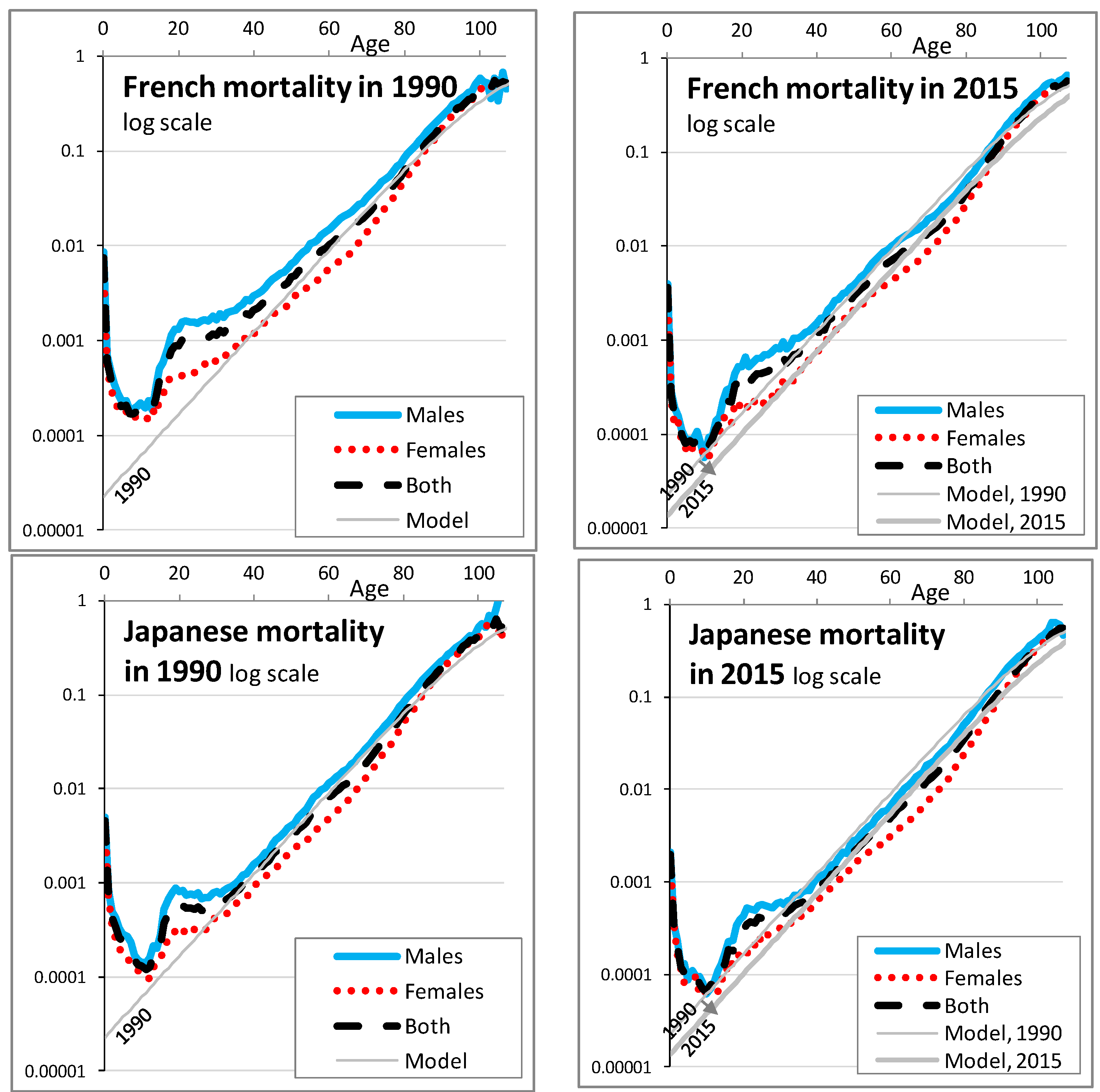
The parameter b can be understood as the natural relative increase of mortality with age. We take b = 10%: this is approximately the historical slope of log-mortality rates between ages 40 and 90, as shown for France, Japan, and the USA for the years 1990 and 2015 in the third and fourth graphs of Figure 1 and in greater detail in Figure A1. Said differently, every increase of age by one year is associated with an increase of mortality risk by approximately 10% of its value.
Figure A1.
Historical mortality rates, for three countries and as modeled. Annual mortality rates are shown in log scale as function of age, for the USA, France and Japan (graphs from top to bottom), in 1990 and in 2015 (graphs on the left and on the right). Each graph shows the mortality of males in a (blue) continuous line, the mortality of females in (red) dots, the mortality of both in (black) dashes and the mortality of the model used in this article in a gray line that is visually straight up to age 85. For the graphs on the right, the mortality of the model in 1990 is added to help visualize the change of mortality between 1990 and 2015.


Other parameters are defined using the concept of static and prospective life expectancy. The prospective life expectancy of a population aged x at time t, , is how long that population lives on average if its mortality rates evolve according to a model. The static life expectancy of that population, , is how long that population lives if mortality rates were not evolving after time t. The word “static” is generally omitted.
Mathematically, the static or prospective life expectancy is the area under the survival curve of the population. As generally done in actuarial science, we approximate that area by consecutive rectangles. The rectangles are centered at every round age (we here name u the age at which survival is estimated; u > x). They are of width one year except the first one, of height 1 and width 0.5 year. This leads to the following formulas where we indicate the computation of survival, S(u), for the sake of clarity:
In the calculation, for practical reasons, we must set a limit for u, rather than infinity. It must be an age that has a negligible probability to be reached according to the model. We arbitrarily take 300 years and have checked that taking 300 or 400 years does not materially affect the estimates here performed.
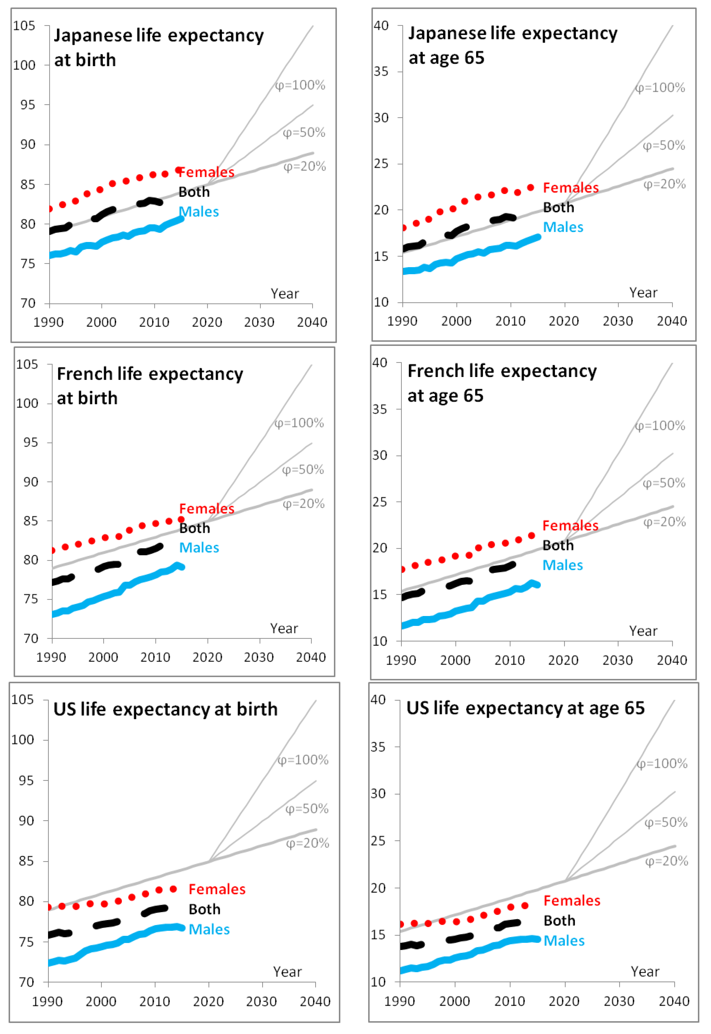
The parameter a can be understood as the initial life expectancy level (or initial mortality level but mortality rates increase when a is decreased). Knowing that what matters most for the article is to simulate various longevity scenarios, we choose one reference country, Japan in our case, and we choose a = 11.3: this provides a reasonable estimate of life expectancy at birth and at age 65 of the Japanese general population in 2020, as shown in the two first graphs of Figure 1 and in greater details in Figure A2.
For the reference country, we chose Japan as it is a long-lived country. We do so because in most countries, the mortality of pensioners would be expected to be lower than general populations owing to their socio-professional levels. This is all the more relevant as the model should represent mortality weighted by amounts (one would expect pension level, health, and low mortality to be positively correlated due to social inequalities) to model capital needs. Still, the model could be adjusted to a particular population by using a different value for a. It is to be noted that further refinements could be made, such as a better mathematical shape of log-mortality as a function of age using for example an adaptation of the model of Heligman and Pollard (1980) as described by Debonneuil (2015). These refinements were deemed unnecessary in the context of this article.
Figure A2.
Static life expectancy at birth and at age 65, for three countries and as modeled. Life expectancy at birth (graphs on the left) and at age 65 (graphs on the right) are shown as function of calendar year, for Japan, France and the USA (graphs from top to bottom). Each graph shows the mortality of males in a (blue) continuous line, the mortality of females in (red) dots, the mortality of both in (black) dashes and the mortality of the model used in this article in portions of gray straight lines. More precisely, = 20% is used for the thick straight line and = 50% and = 100% is used for the two thin straight lines that start in 2020.

Let us now discuss , which represents the longevity trend. As explained for a broader range of models by Bongaarts (2005), Equation (1) produces annual increases of life expectancy at birth by years because increasing t by 1 year produces the same mortality rates as decreasing x by year (and because at birth, where decreasing x does not make sense, the model produces negligible mortality rates compared to adult mortality rates). For example, to model life expectancy increases of a quarter every year we would consider . This is a clear behavior compared to various actuarial models, such as the model from Lee and Carter (1992), that are often believed to extrapolate historical trends with a neutral view but actually tend to produce decelerating life expectancies and no longevity improvements ultimately (see Bongaarts 2005; and Debonneuil et al. 2017). Another clear behavior of the model is to produce mortality improvements that are at young ages (because we use b = 1/10), so 2.5% in the example of an additional quarter per year. These mortality improvements gradually lower with age without forcing mortality improvements by age to be constant over time.
As highlighted in the first two graphs of Figure 1 for 3 countries and by Debonneuil et al. (2017) for a range of 24 countries, fits the current longevity trend. This why we consider = 20% before t = 0. Debonneuil et al. (2017) used a similar model, “Best Practice Trend”, that is more complex to express in terms of annual mortality rates but that has the same longevity trend feature.
However, the future longevity trend may be different. A wide range of potential longevity increases can happen as we have seen, so we use a lognormal distribution of . Its median is 20% to have a 50% chance of greater or lower longevity trend. The probability density function is then the one shown in Equation (2). Considering a possible wave of solutions for age-related conditions in the coming decades, we set the standard-deviation to 1. This leads to a 5% probability that > 1 (precisely, based on 10 million simulations of , we measure a probability of 5.38%). Over long periods of time, the latter corresponds to people enjoying better health and reduced mortality risks as time goes, for example, because of the emergence and progressive generalization of tissue regeneration techniques. The future is unknown and some authors may argue that this probability of 5% is not reflective of future longevity trends. This is why at times in the article, we consider four specific longevity scenarios that could be weighted as a mean to represent other distributions of longevity risk: = 0% (no improvement in the future), = 20% (historical trend), = 50% (wave of anti-aging solutions) and = 80% (strong solutions to aging).
The relevance of the = 50% and scenarios and the relevance of a 5% probability of having = 100% can be partially appreciated in light of historical annual increases of life expectancy that followed large implementations of biomedical discoveries. We attribute a value of to them because models annual increases of life expectancy. Around 1950, Japan had a trend above = 100%, suggesting that high trends are possible when solutions for better health are known and are implemented. In the last decades, south Asian countries of Malaysia, Philippines, Vietnam, Laos, and Bangladesh (see Carbonnier et al. 2013) have experienced an increase above 50%. During approximately 70 years after the microbial communications of Louis Pasteur, was around 30% in long-lived countries (see Vallin and Meslé 2010). The Pasteur example is particularly interesting as improving hygiene requires complex cultural, technological, and urbanization changes: it can be foreseen that using anti-aging therapies once available is a faster process.
Appendix B. Investigation of the Current Rate of Return of Pharmaceutical Developments
Biology of aging may be reaching the clinics now and in the forthcoming decades, which should, in principle, boost the pharmaceutical industry. However, for now a crisis is declared on the pharmaceutical side, with reported strong increases in research and development investments in the last decades, high cost of risk for investors, but strong decreases in success rates of drug development (see Scannell et al. 2012). Reported estimates of average research and developments cost are $802 M (see DiMasi et al. 2003) per successful drug, including the cost of failures, or more recently $2558 M (see DiMasi et al. 2016). Such numbers are debated to be less than $59 M and it is suggested that most publicly available data in the field are biased (see Light and Warburton 2011; and Lazonick et al. 2017).
In this delicate context of non-communicated cost structure, the first megafund studies conducted sophisticated analysis of historical drug developments.
For the cancer megafund (Fernandez et al. 2012, in Supplementary materials), a Markovian model was developed for simulations as well as two very simple models to explain the orders of magnitude of profitability: a model for blockbusters (drugs with annual revenues of more than $1 Bn) and a model for non-blockbusters. These two models consist in an initial investment , $200 M and $100 M, respectively, leading ten years later to a gain , $12.3 B and $3.1 B respectively, with a probability, , of 5% and 10%, respectively. When using Equation (13), it happens that with these numerical assumptions the two models lead to the same annualized return of 11.9%.
For the case of a megafund against rare diseases, one would expect smaller investments and smaller gains: small clinical trial sizes may be accepted given the reduced number of patients, and the drugs would be commercialized to less patients. After detailed analyses (see Fagnan et al. 2014), including refinements to be less dependent on industry averages (see Fagnan et al. 2015), the costs for preclinical trials, phase I, and II (elements of ) are respectively estimated at about $3 M, $3 M and $8 M , the resulting values (elements of ) are estimated at about $7 M, $23 M and $57 M and success probabilities (elements of ) at about 80%, 87%, and 53%. Put together, the final annualized rate of return is estimated to be between 12% and 15% (see Fagnan et al. 2015).
Recently, the average costs, probabilities of success and durations of clinical developments have become much clearer following articles in 2016, 2017, and 2018 from teams with large amounts of data and incentives (see Sertkaya et al. 2016; Martin et al. 2017; Wong et al. 2018). As a result, it becomes easier to estimate the megafund profitability by distinguishing cost, success rate, and gains of pharmaceutical developments. We perform this analysis with a particular focus on the USA as it is by far the country with the most clinical development (see Thiers et al. 2008).
The average US cost of a phase I, II, and III in the USA is, respectively, $4 M, $13 M, and $20 M and the cost for the FDA approval step is smaller (see Sertkaya et al. 2016). Similarly, the medium cost for major biopharma companies is respectively $3.4 M, $8.6 M, and $21.4 M (not specific to the USA; see Martin et al. 2017). When summing these numbers, in both cases the cost of a drug development that goes through two phase I, two phase II, one phase III, and one FDA approval is about $50 M, or $0.05 Bn (we considered two phases I and two phases II in this amount to represent additional costs such as reproducibility tests of biology of aging results). This order of magnitude is for all therapeutic areas on average as well as for the specific case of oncology (see Sertkaya et al. 2016).
The success rate for a compound in phase I to reach the market is estimated by Wong et al. (2018) at 14% (66.4% to reach phase II and then 58.3% to reach phase III and then 59.3% to reach approval; the model that assumes at least 1 phase I, 1 phase II, 1 phase III if one of the phases is lacking in the data). It is greater than previous estimates at 9.1% (see Thomas et al. 2016). It particular, it includes significantly higher success rates since 2013. Whether the later increase comes from a bias in their model or a real recent change, our further investigation based on open data does not confirm this trend very clearly, so we will take a slightly prudent hypothesis in that respect.
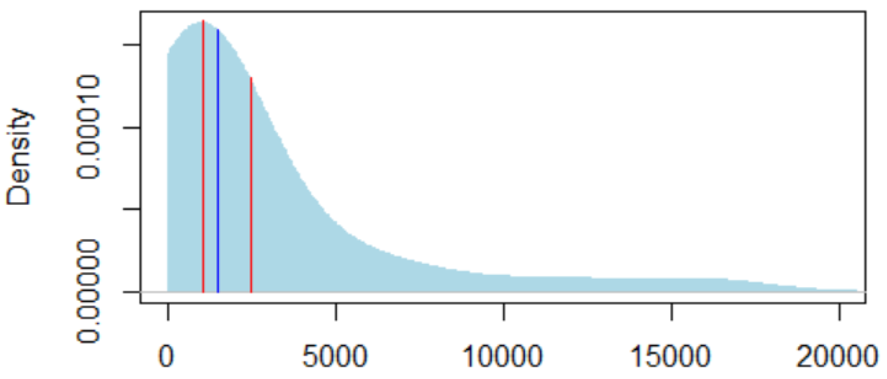
We then estimate the megafund gain of selling the intellectual property to pharmaceutical companies by referring to the valuations obtained by Royal Pharma. Royal Pharma is a company that buys biomedical intellectual property and sells it to pharmaceutical companies. The sales amounts are reported online (Royal Pharma portfolio) and Figure A3 shows the distribution of amounts obtained. The median is $1.03 Bn. The average is $2.48 Bn. Two amounts are greater than $10 Bn, and if removed, the average becomes $1.66 Bn. With a margin of prudence, as a megafund might not be as efficient as Royal Pharma in optimizing sales, we considered a gain of $1.5 Bn per successful pharmaceutical development.
Figure A3.
Estimated gain per successful drug development based on Royalty Pharma sales. The x-axis of the two red vertical bars are the mean (2.48 bn$, on the right) and the median ($1.03 bn, on the left) of the sales amounts, in $M. The light blue shade is the density of the sales amount, using a smoothing gaussian kernel whose bandwidth is half of the sales standard deviation. The blue vertical bar, between the two red horizontal bars, is the gain we consider for investors in the megafund, under current longevity trends ($1.5 Bn).

Combining costs of $50 M, a success rate of 14% and gains of $1500 M in Equation (13) leads to an annualized return of (14%*1500/50)0.1-1 = 15.4%. Using a slightly lower success rate as seen above, of 12%, and a greater cost to include management fees and carried interest, as reminded by Phalippou (2010), of $60 M, leads to an annualized return of 11.6%. This is not far from the 11.9% annualized return suggested by Fernandez et al. (2012) in the case of a cancer megafund.
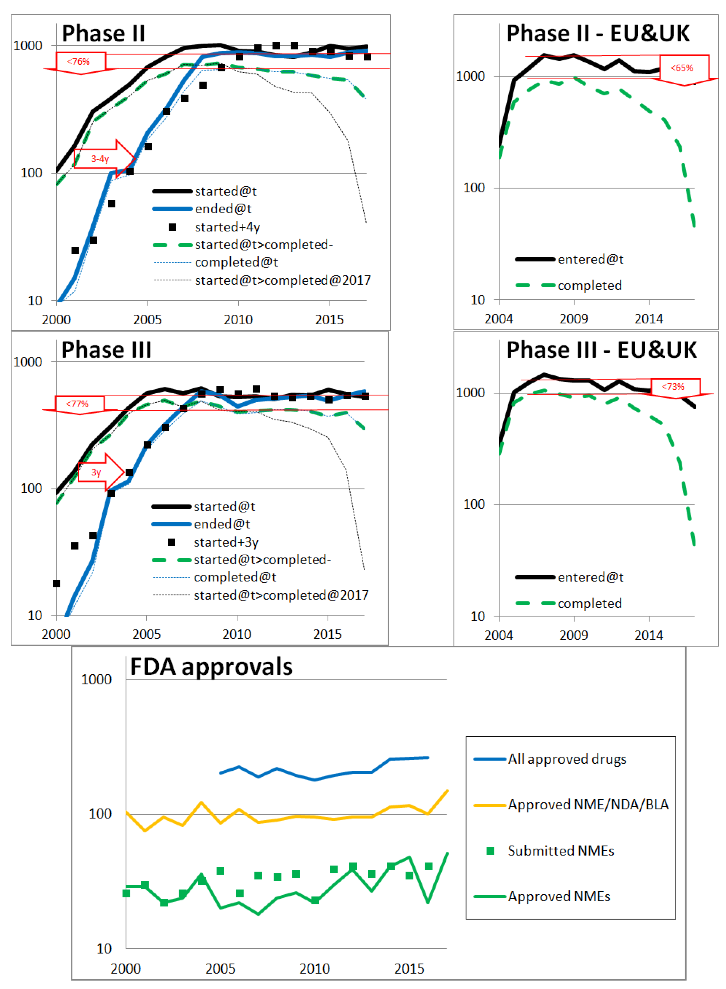
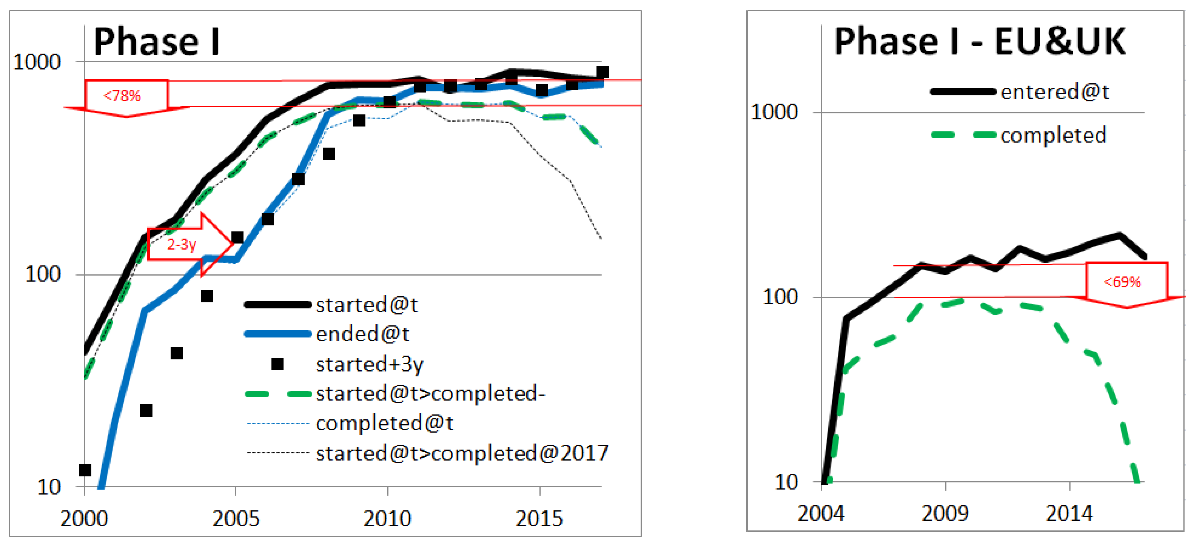
All these investigations are based on the literature. As we have seen, there is conflicting data in the literature. In order to better decipher the right orders of magnitude, we analyzed the evolution of pharmaceutical developments based on open data. More precisely, we followed the evolution of clinical trials and FDA approvals in the USA, Europe, and the UK. We investigated the main types of clinical trials: Phase I, II, and III. Phase I trials are conducted with a small number of patients (20–80) mainly to test safety and first side effects, phase II trials involve a larger group of patients (100–300) to determine efficacy against a placebo, and to further evaluate side effects, and phase III trials are conducted with a large group of patients (1000–3000) to confirm efficacy and safety, and to compare the drug or treatment with existing ones. The results are shown in in Figure A4: various indicators of drug development are particularly stable which suggests that the pharmaceutical research and development field is relatively stable.
In particular, in the first 3 graphs on the left of Figure A4 the number of declared new clinical trials in the USA, according to clinicaltrials.gov, is stable since 2008 and roughly equal to the number of clinical trials ended: there are as many clinical trials starting as ending. Both the stability and the equality at a plateau suggest that, contrary to what one may read, the number of clinical trials of each type has remained very stable. Since declaring clinical trials in clinicaltrials.gov is needed to publish in the USA, it is a relatively reliable source.
Figure A4.
Pharmaceutical drug development indicators based on open data: clinicaltrials.gov, clinicaltrialsregister.eu, Drugs@FDA, and accessdata.fda.gov. The three first graphs on the left show numbers of USA clinical trials per calendar year, t, for respectively Phase I, Phase II, and Phase III reporting by the pharmaceutical industry according to clinicaltrials.gov. The Y-axis is a logarithmic scale. For each of them, the top (black) thick and continuous curve is the number of clinical trials started each year (first participant enrolled). The other thick continuous curve (in blue) is the number of clinical trials ended each year (primary completion data: last participant providing data for the primary outcome measure). A decay of 3 or 4 years of the first (black) curve is represented in (black) squares to see how well it compares with the second (blue) curve: the resulting estimated length of clinical trials is indicated in the (red) arrow pointing the right. The (black) thin dashed curve that plunges on the right side is the number of clinical trials started each year AND completed before 2018. The plateaus observed with the first two lines and the latter two lines, underlined (in red), differ due to the non-100% completion rate, as measured in the arrows pointing down (with a “<” sign with respect to success rate). The three graphs on the right side are equivalent slides but for Europe and the UK, based on clinicaltrialsregister.eu; clinicaltrialsregister.eu is more recent than clinicaltrials.gov and does not provide the same filters, so we only rely on clinical trials started each year, completed since or not. The last graph shows the accepted drugs of different types in the USA, by the FDA, every year. The top (blue) line represents any type of new drug accepted (United States Government Accountability Office, 2017). The middle yellow curve represents approvals for some specific types of treatments: New Molecular Entities (NME), New Drug Applications, Biologic License Applications (types 1–8 in (Drugs@FDA 2018)). The bottom green curve represents NMEs only. The number of NME submissions (accessdata.fda.gov, 2018) is shown in green squares.

Other observations in Figure A4 are less striking but they all similarly suggest a good stability of pharmaceutical developments, which contributed to our estimates of financial returns.
It is expected that the two curves are at a lower level before 2008 as clinicaltrials.gov is recent. The decay of the curves gives an estimate of the duration of the clinical trials including enrollment time: 2–3 years for Phase I, 3–4 for Phase II, and 3 for Phase III.
The rate of normal completion of clinical trials (defined in clinicaltrials.gov as having the “last subject, last visit” occurred) is estimated by the ratio between the number of completed trials and the number of trials. Even though the lines of completed clinical trials have bias both on the left (since clinicaltrials.gov is recent) and on the right (since not all trials have had the time to end), a plateau can again be seen. Looking at the difference of the plateaus (number of clinical trials and number of completed clinical trials), the data suggests that the rate of normal completion is stable for the different phases. These rates are approximately 15% greater than the success rate estimated by Wong et al. (2018), which is not incoherent.
The European and UK data suggests similar patterns although the more recent and not mandatory declaration in clinicaltrialsregister.eu make it less reliable: it is difficult to judge in what degree the results are different from the USA.
The last graph of Figure A4 indicates that the success rate from starting a Phase III—the most costly phase—to approval is greater than 50%: out of 400 annually completed phase III trials, 200 new drugs are accepted per year. This is more than is often perceived by communications in the field. Lastly, the squares are close to the curve and suggest that the FDA approval rate for new molecular entities is 89% over 1996–2016. All this is factored into the non-negligible returns we estimated. The advantage of such open data is that anyone can reproduce the computation to appreciate that pharmaceutical successes are not rare and that investing in pharmaceutical developments is reasonably financially attractive.
Appendix C. List of Figures, Tables, and Variables in the Article
In order to accompany the understanding of the concepts of this article, this part lists figures, tables, and variables by theme: “Longevity model”, “Returns of pharmaceutical developments”, and “Pension fund needed capital”.

Table A1.
Figures.
| Theme | Figure | Name |
|---|---|---|
| Longevity model | 1 | Characteristics of the chosen longevity model |
| A1 | Historical mortality rates, for three countries and as modeled | |
| A2 | Static life expectancy at birth and at age 65, for three countries and as modeled | |
| developments | A3 | Estimated gain per successful drug development based on Royalty Pharma sales |
| pharmaceutical | A4 | Pharmaceutical drug development indicators based on open data: clinicaltrials.gov, clinicaltrialsregister.eu, Drugs@FDA and accessdata.fda.gov |
| Returns of | 3 | Megafund annualized return r as a function of longevity trend φ |
| 4 | Annualized equity return i as a function of longevity trend φ | |
| Pension fund needed capital | 2 | Needed prudential capital depending on the future longevity trend (or lack of) expressed as a proportion of the initial wealth |
| 5 | Needed prudential capital, expressed as a proportion of the initial wealth, depending on the future longevity trend and on investments in a longevity megafund |
Table A2.
Tables.
| Theme | Table | Name |
|---|---|---|
| Pension fund needed capital | 1 | Contributions by age tranche |
| 2 | Needed prudential capital, expressed as a proportion of the initial wealth, depending on investments in a megafund |
Table A3.
Variables.
| Theme | Variable | Name | Definition |
|---|---|---|---|
| Longevity model | Level of longevity | Equation (1) | |
| Ageing rate | Equation (1) | ||
| Age in years | Equation (1) | ||
| Longevity trend | Equation (1) | ||
| Year (t = 0 corresponds to 2020) | Equation (1) | ||
| Annual mortality rate at age x and time t | Equation (1) | ||
| Standard deviation of potential longevity trends | Equation (2) | ||
| Prospective life expectancy at age x and time t | Equation (A1) | ||
| Static life expectancy at age x and time t | Equation (A2) | ||
| initial investment | Equation (12) | ||
| gain ten years later | Equation (12) | ||
| probability of success | Equation (12) | ||
| Returns of pharmaceutical developments | 10-year return | Equation (12) | |
| annualized return | Equations (12) and (16) | ||
| evolution of with longevity | Equations (14) and (15) | ||
| parameter to ajust the expected level of | Equation (14) | ||
| correlation between and longevity | Equation (15) | ||
| residual performance of the megafund | Equation (14) | ||
| I | annualized return of the equity tranche | Equation (17) | |
| equity percentage of investments in the megafund | Equation (17) | ||
| Pension fund needed capital | number of persons aged x at time t | Equation (3) | |
| accumulated capital for the group of persons aged x at t | Equations (6) and (7) | ||
| i1, i2, i3 | expected annual return of contributions by age tranche | Table 1, Equation (4) | |
| σ1, σ2, σ3 | standard deviation of the annual returns by age tranche | Table 1, Equation (4) | |
| ik,t | annual return of contributions by age tranche and year | Table 1, Equation (5) | |
| initial wealth of the pension fund | Equation (8) | ||
| annual benefit paid to the workers who retire at time t | Equation (9) | ||
| needed prudential capital for a given scenario | Equation (10) | ||
| K | needed prudential capital | Equation (11) | |
| p1, p2, p3 | percentage of investments in the equity tranche by age tranche | Section 4.2 |
References
- Antolin, Pablo, and Jessica Mosher. 2014. Mortality Assumptions and Longevity Risk. Paris: OECD, Working Party on Private Pensions. [Google Scholar]
- Arias, Elizabeth, Melonie Heron, and Betzaida Tejada-Vera. 2013. United States Life Tables Eliminating Certain Causes of Death, 1999–2001. National Vital Statistics Reports 61: 1–128. [Google Scholar] [PubMed]
- Ayyadevara, Srinivas, Ramani Alla, John Thaden, and Robert Joseph Shmookler Reis. 2008. Remarkable longevity and stress resistance of nematode PI3K-null mutants. Aging Cell 7: 13–22. [Google Scholar] [CrossRef] [PubMed] [Green Version]
- Barardo, Diogo, Daniel Thornton, Harikrishnan Thoppil, Michael Walsh, Samim Sharifi, Susana Ferreira, Andreja Anžič, Maria Fernandes, Patrick Monteiro, Tjaša Grum, and et al. 2017. The DrugAge database of aging-related drugs. Aging Cell 16: 594–97. [Google Scholar] [CrossRef] [PubMed]
- Bartke, Andrzej, Michael Bonkowski, and Michal Masternak. 2008. How diet interacts with longevity genes—Review. Hormones 7: 17–23. [Google Scholar] [CrossRef] [PubMed]
- Ben-Haim, Moshe Shay, Yariv Kanfi, Sarah J Mitchell, Noam Maoz, Kelli L Vaughan, Ninette Amariglio, Batia Lerrer, Rafael de Cabo, Gideon Rechavi, and Haim Y Cohen. 2017. Breaking the Ceiling of Human Maximal Lifespan. The Journals of Gerontology. Series A, Biological Sciences and Medical Sciences. [Google Scholar] [CrossRef] [PubMed]
- Boissel, François-Henri. 2013. The cancer megafund: mathematical modeling needed to gauge risk. Nature Biotechnology 31: 494. [Google Scholar] [CrossRef] [PubMed]
- Bongaarts, John. 2005. Long-Range Trends in Adult Mortality: Models and projection methods. Demography 42: 23–49. [Google Scholar] [CrossRef] [PubMed]
- Broadbent, John, Michael Palumbo, and Elizabeth Woodman. 2006. The Shift from Defined Benefit to Defined Contribution Pension Plans–Implications for Asset Allocation and Risk Management; Sydney: Reserve Bank of Australia, Washington: Board of Governors of the Federal Reserve System, Ottawa: Bank of Canada, pp. 1–54.
- Carbonnier, Gilles, Pavel Chakraborty, Emmanuel Dalle Mulle, and Cartografare il presente. 2013. Asian and African Development Trajectories—Revisiting Facts and Figures. International Development Policy. Working papers. Geneva: Graduate Institute of International and Development Studies. [Google Scholar] [CrossRef]
- Casquillas, Guilhem Velvé. 2016. Human Longevity: The Giants. Available online: LongLongLife.org (accessed on 28 April 2018).
- De Magalhães, João Pedro, Michael Stevens, and Daniel Thornton. 2017. The business of anti-aging science. Trends in Biotechnology 35: 1062–73. [Google Scholar] [CrossRef] [PubMed]
- Debonneuil, Edouard. 2015. Modèle Paramétrique de Mortalité en Fonction de L’âge, Pour des Applications à des Portefeuilles de Retraite. Actuarial Memorandum, ISFA. Available online: http://www.ressources-actuarielles.net (accessed on 28 April 2018).
- Debonneuil, Edouard, Lise He, Jessica Mosher, and Nathalie Weiss. 2011. Longevity Risk: Setting the Scene. London: Risk books. [Google Scholar]
- Debonneuil, Edouard, Frédéric Planchet, and Stéphane Loisel. 2017. Do actuaries believe in longevity deceleration? Insurance: Mathematics and Economics 31: 373–93. [Google Scholar] [CrossRef]
- Devlin, Nancy. 2003. Does NICE Have a Cost Effectiveness Threshold and What Other Factors Influence Its Decisions? A Discrete Choice Analysis. Report No. 03/01. London: Department of Economics, City University London. [Google Scholar]
- DiMasi, Joseph A., Ronald W. Hansen, and Henry G. Grabowski. 2003. The price of innovation: New estimates of drug development costs. Journal of Health Economics 22: 151–85. [Google Scholar] [CrossRef]
- DiMasi, Joseph A., Henry G. Grabowski, and Ronald W. Hansen. 2016. Innovation in the pharmaceutical industry: New estimates of R&D costs. Journal of Health Economics 47: 20–33. [Google Scholar] [PubMed] [Green Version]
- Drugs@FDA. 2018. Available online: http://www.fda.gov/drugsatfda (accessed on 28 April 2018).
- Dublin, Louis Israel. 1928. Health and Wealth. A Survey of the Economics of World Health. New York: Harper, p. 361. [Google Scholar]
- El Karoui, Nicole, Caroline Hillairet, and Mohamed Mrad. 2014. Affine long-term yield curves: An application of the Ramsey rule with progressive utility. Journal of Financial Engineering, 1. [Google Scholar] [CrossRef]
- Fagnan, David E., Austin A. Gromatzky, Roger M. Stein, Jose-Maria Fernandez, and Andrew W. Lo. 2014. Financing drug discovery for orphan diseases. Drug Discovery Today 19: 533–38. [Google Scholar] [CrossRef] [PubMed]
- Fagnan, David E., N NoraYang, John C McKew, and Andrew W. Lo. 2015. Financing translation: Analysis of the NCATS rare-diseases portfolio. Science Translational Medicine 7: 276ps3. [Google Scholar] [CrossRef] [PubMed]
- Fahy, Gregory M. 2003. Apparent induction of partial thymic regeneration in a normal human subject: A case report. Journal of Anti-Aging Medicine 6: 219–27. [Google Scholar] [CrossRef] [PubMed]
- Fernandez, Jose-Maria, Roger M. Stein, and Andrew W. Lo. 2012. Commercializing biomedical research through securitization techniques. Nature Biotechnology 30: 964–75. [Google Scholar] [CrossRef] [PubMed] [Green Version]
- Gavrilov, Leonid A., Vyacheslav N. Krut’ko, and Natalia S. Gavrilova. 2017. The future of human longevity. Gerontology 63: 524–26. [Google Scholar] [CrossRef] [PubMed]
- Guibert, Quentin, Frédéric Planchet, and Michaël Schwarzinger. 2017. Mesure de l’espérance de vie sans dépendance en France. Forthcoming. [Google Scholar]
- Heligman, Larry, and John H. Pollard. 1980. The age pattern of mortality. Journal of the Institute of Actuaries 107: 49–82. [Google Scholar] [CrossRef]
- House of Commons Work, Pensions Committee. 2016. Defined Benefit Pension Schemes. Sixth Report of Session 2016–17. London: House of Commons Work and Pensions Committee. [Google Scholar]
- Howard, David H., Peter B. Bach, Ernst R. Berndt, and Rena M. Conti. 2015. Pricing in the market for anticancer drugs. Journal of Economic Perspectives 29: 139–62. [Google Scholar] [CrossRef] [PubMed]
- Hull, John. 2016. Funding Long Shots. In Rotman School of Management Working paper No. 2773108. Toronto: Rotman School of Management, University of Toronto. [Google Scholar] [CrossRef]
- Kantor, Elizabeth D., Colin D. Rehm, Jennifer S. Haas, Andrew T. Chan, and Edward L. Giovannucc. 2015. Trends in prescription drug use among adults in the United States from 1999–2012. JAMA 314: 1818–30. [Google Scholar] [CrossRef] [PubMed]
- Kenyon, Cynthia J. 2010. The genetics of ageing. Nature 464: 504–12. [Google Scholar] [CrossRef] [PubMed]
- Lazonick, William, Matt Hopkins, Ken Jacobson, Mustafa Sakinc, and Oner Tulum. 2017. US Pharma’s Financialized Business Model. Institute for New Economic Thinking Working Paper Series No. 60; New York: Institute for New Economic. [Google Scholar]
- Lee, Ronald D., and Lawrence R. Carter. 1992. Modeling and forecasting U.S. mortality. Journal of the American Statistical Association 87: 659–71. [Google Scholar] [CrossRef]
- Light, Donald W., and Rebecca Warburton. 2011. Demythologizing the high costs of pharmaceutical research. BioSocieties 6: 34–50. [Google Scholar] [CrossRef]
- Lo, Andrew W. 2015. Can Financial Engineering Cure Cancer? San Bruno: YouTube. Video. [Google Scholar]
- Lo, Andrew W., and Sourya V. Naraharisetti. 2014. New Financing Methods in the Biopharma Industry: A Case Study of Royalty Pharma, INC. Journal of Investment Management 12: 4–19. [Google Scholar] [CrossRef]
- Lo, Andrew W., Carloe Ho, Jayna Cummings, and Kenneth S. Kosik. 2014. Parallel discovery of Alzheimer’s therapeutics. Science Translational Medicine 6: 241cm5. [Google Scholar] [CrossRef] [PubMed]
- MacMinn, Richard D., and Nan Zhu. 2017. Hedging Longevity Risk in Life Settlements Using Biomedical Research-Backed Obligations. Journal of Risk and Insurance 84: 439–58. [Google Scholar] [CrossRef]
- Marko, Nicholas F. 2013. The cancer megafund: determinants of success. Nature Biotechnoloy 31: 492–94. [Google Scholar] [CrossRef] [PubMed]
- Martin, George M., Kelly LaMarco, Evelyn Strauss, and Katrina Kelner. 2003. Research on aging: The end of the beginning. Science 299: 1339–41. [Google Scholar] [CrossRef] [PubMed]
- Martin, Linda, Melissa Hutchens, Conrad Hawkins, and Alaina Radnov. 2017. How much do clinical trials cost? Nature Reviews Drug Discovery 16: 381–90. [Google Scholar] [CrossRef] [PubMed]
- Mellon, Jim, and Al Chalabi. 2017. Juvenescence: Investing in the Age of Longevity. Hampshire: Harriman House Limited. [Google Scholar]
- Mendelsohn, Andrew R., James W. Larrick, and Jennifer L. Lei. 2017. Rejuvenation by Partial Reprogramming of the Epigenome. Rejuvenation Research 20: 146–50. [Google Scholar] [CrossRef] [PubMed]
- Mir, Tanveer Ahmad, and Makoto Nakamura. 2017. Three-Dimensional Bioprinting: Toward the Era of Manufacturing Human Organs as Spare Parts for Healthcare and Medicine. Tissue Engineering Part B: Reviews 23: 245–56. [Google Scholar] [CrossRef] [PubMed]
- Moskalev, Alexey, Vladimir Anisimov, Aleksander Aliper, Artem Artemov, Khusru Asadullah, Daniel Belsky, Ancha Baranova, Aubrey de Grey, Vishwa Deep Dixit, Edouard Debonneuil, and et al. 2017. A review of the biomedical innovations for healthy longevity. Aging (Albany NY) 9: 7–25. [Google Scholar] [CrossRef] [Green Version]
- Mosteiro, Lluc, Cristina Pantoja, Noelia Alcazar, Rosa M. Marión, Dafni Chondronasiou, Miguel Rovira, Pablo J. Fernandez-Marcos, Maribel Muñoz-Martin, Carmen Blanco-Aparicio, Joaquin Pastor, and et al. 2016. Tissue damage and senescence provide critical signals for cellular reprogramming in vivo. Science, 354. [Google Scholar] [CrossRef] [PubMed]
- Murphy, Kevin M., and Robert H. Topel. 2006. The value of health and longevity. Journal of political Economy 114: 871–904. [Google Scholar] [CrossRef]
- Neumann, Peter J., Joshua T. Cohen, and Milton C. Weinstein. 2014. Updating cost-effectiveness—The curious resilience of the $50,000-per-QALY threshold. New England Journal of Medicine 371: 796–97. [Google Scholar] [CrossRef] [PubMed]
- Ocampo, Alejandro, Pradeep Reddy, Paloma Martinez-Redondo, Aida Platero-Luengo, Fumiyuki Hatanaka, Tomoaki Hishida, Mo Li, David Lam, Masakazu Kurita, Ergin Beyret, and et al. 2016. In Vivo Amelioration of Age-Associated Hallmarks by Partial Reprogramming. Cell 167: 1719–33. [Google Scholar] [CrossRef] [PubMed]
- OECD. 2017. Health at a Glance: OECD Indicators. Paris: OECD Publishing, Available online: http://dx.doi.org/10.1787/health_glance-2017-en (accessed on 28 April 2018).
- Olshansky, S. Jay, Bruce A. Carnes, and Christine Cassel. 1990. In Search of Methuselah: Estimating the Upper Limits to Human Longevity. Science 250: 634–40. [Google Scholar] [CrossRef] [PubMed]
- Phalippou, Ludovic. 2010. Investing in Private Equity Funds: A Survey. Charlottesville: The Research Foundation of CFA Institute. [Google Scholar]
- Pifferi, Fabien, Jérémy Terrien, Julia Marchal, Alexandre Dal-Pan, Fathia Djelti, Isabelle Hardy, Sabine Chahory, Nathalie Cordonnier, Loïc Desquilbet, Murielle Hurion, and et al. 2018. Caloric restriction increases lifespan but affects brain integrity in grey mouse lemur primates. Communications Biology 1: 30. [Google Scholar] [CrossRef]
- Pratt, Chelsea. 2016. 5 Private Longevity Stocks to Watch: From Calico to Genescient. Investing News. December 22. Available online: https://investingnews.com/daily/life-science-investing/longevity-investing/top-longevity-stocks-alkahest-calico-elysium-health-navitor/ (accessed on 28 April 2018).
- Ravnic, Dino J., Ashley N. Leberfinger, Srinivas V. Koduru, Monika Hospodiuk, Kazim K. Moncal, Pallab Datta, Madhuri Dey, Elias Rizk, and Ibrahim T. Ozbolat. 2017. Transplantation of Bioprinted Tissues and Organs: Technical and Clinical Challenges and Future Perspectives. Annals of Surgery 266: 48–58. [Google Scholar] [CrossRef] [PubMed]
- Roman, Pablo, and Alberto Ruiz-Cantero. 2017. Polypathology, an emerging phenomenon and a challenge for healthcare systems. Revista Clinica Espanola 217: 229–37. [Google Scholar] [CrossRef] [PubMed]
- Scannell, Jack W., Alex Blanckley, Helen Boldon, and Brian Warrington. 2012. Diagnosing the decline in pharmaceutical R&D efficiency. Nature Reviews Drug Discovery 11: 191–200. [Google Scholar] [PubMed]
- Sertkaya, Aylin, Hui-Hsing Wong, Amber Jessup, and Trinidad Beleche. 2016. Key cost drivers of pharmaceutical clinical trials in the United States. Clinical Trials 13: 117–26. [Google Scholar] [CrossRef] [PubMed]
- Stein, Roger M. 2016. A Simple Hedge for Longevity Risk and Reimbursement Risk Using Research-Backed Obligations. MIT Sloan Research Paper No. 5165-16. Cambridge: MIT Sloan School of Management. [Google Scholar]
- Stewart, Jeffrey J., Peter N. Allison, and Ronald S. Johnson. 2001. Putting a price on biotechnology. Nature Biotechnology 19: 813–17. [Google Scholar] [CrossRef] [PubMed]
- Swedish Agency for Growth Policy Analysis. 2017. Towards a Swedish Megafund for Life Science Innovation; Tillväxtanalysis 2017/089. Östersund: Swedish Agency for Growth Policy Analysis.
- Tenenbaum, Jay M. 2013. The cancer megafund: A catalyst for disruptive innovation. Nature Biotechnology 31: 491–92. [Google Scholar] [CrossRef] [PubMed]
- Tengs, Tammy O., Miriam E. Adams, Joseph S. Pliskin, Dana Gelb Safran, Joanna E. Siegel, Milton C. Weinstein, and John D. Graham. 1995. Five-hundred life-saving interventions and their cost-effectiveness. Risk Analysis 15: 369–90. [Google Scholar] [CrossRef] [PubMed]
- Thiem, Ulrich, Timo Hinrichs, Christiane A Müller, Stefanie Holt-Noreiks, Alexander Nagl, Claudio Bucchi, Ulrike Trampisch, Anna Moschny, Petra Platen, Erika Penner, and et al. 2011. Prerequisites for a new health care model for elderly people with multiple morbidities: Results and conclusions from 3 years of research in the PRISCUS consortium. Zeitschrift Fur Gerontologie Und Geriatrie 44: 101–12. [Google Scholar] [CrossRef] [PubMed]
- Thiers, Fabio A., Anthony J. Sinskey, and Ernst R. Berndt. 2008. Trends in the Globalization of Clinical Trials. Cambridge: MIT. [Google Scholar]
- Thomas, David W., Justin Burns, John Audette, Adam Carrol, Corey Dow-Hygelund, and Michael Hay. 2016. Clinical Development Success Rates 2006–2015. San Diego: Biomedtracker. [Google Scholar]
- Transparency Market Research. 2014. Anti-Aging Market (Anti-Wrinkle Products, Hair Color, Hair Restoration Treatment, Breast Augmentation and Radio Frequency devices)—Global Industry Analysis, Size, Share, Growth, Trends and Forecast, 2013–2019. Albany: Transparency Market Research. [Google Scholar]
- US Department of Labor. 2016. Types of Retirement Plans. Available online: https://www.dol.gov/general/topic/retirement/typesofplans (accessed on 28 April 2018).
- Vallin, Jacques, and France Meslé. 2010. Espérance de vie: Peut-on gagner trois mois par an indéfiniment? Population & Sociétés. No. 473. Available online: http://alexandre.cor-retraites.fr/IMG/pdf/doc-2305.pdf (accessed on 28 April 2018).
- Vaupel, James W. 2010. Biodemography of human ageing. Nature 464: 536–42. [Google Scholar] [CrossRef] [PubMed]
- Vijg, Jan, and Eric Le Bourg. 2017. Aging and the inevitable limit to human life span. Gerontology 63: 432–34. [Google Scholar] [CrossRef] [PubMed]
- Wong, Chi Heem, Kien Wei Siah, and Andrew W. Lo. 2018. Estimate of clinical trial success rates and related parameters. Biostatistics. [Google Scholar] [CrossRef] [PubMed]
- Yang, Xianjin, Edouard Debonneuil, Alex Zhavoronkov, and Bud Mishra. 2016. Cancer megafunds with in silico and in vitro validation: Accelerating cancer drug discovery via financial engineering without financial crisis. Oncotarget 7: 57671–78. [Google Scholar] [CrossRef] [PubMed]
- Zhavoronkov, Alexander, Edouard Debonneuil, Nawazish Mirza, and Igor Artyuhov. 2012. Evaluating the impact of recent advances in biomedical sciences and the possible mortality decreases on the future of health care and Social Security in the United States. Pensions 17: 241–51. [Google Scholar] [CrossRef]
- Zion Market Research. 2017. Anti-Aging Market (Baby Boomer, Generation X and Generation Y), by Product (Botox, Anti-Wrinkle Products, Anti-Stretch Mark Products, and Others), by Services (Anti-Pigmentation Therapy, Anti-Adult Acne Therapy, Breast Augmentation, Liposuction, Chemical Peel, Hair Restoration Treatment, and Others), by Device (Microdermabrasion, Laser Aesthetics, Anti-Cellulite Treatment and Anti-Aging Radio Frequency Devices): Global Industry Perspective, Comprehensive Analysis, Size, Share, Growth, Segment, Trends and Forecast, 2015–2021. Pune: Zion Market Research. [Google Scholar]
| 1 | The 50% correlation is not critical for the model as longevity risk is the main risk; setting the correlation to 0% did not materially affect results |
Figure 1.
Characteristics of the chosen longevity model. In the first two graphs, remaining life expectancy at respectively birth and age 65 is computed from year 1990 to 2040 based on the model (see Equation (1)), in gray lines using different values of φ as written, and from 1990 to 2015 for specific countries based on historical data (more precisely based on the mortality rates estimates provided by the Human Mortality Database): Japan in (red) short dashes, France in (blue) continuous lines, and the USA in black long dashes. As expected, life expectancies are greater in Japan than in France and lower in the USA. The model fits life expectancy and mortality rates of Japan. The same style of lines is used for the next two graphs, that represent the mortality rate at different ages in log scale, for the years 1990 and 2015, respectively. The model matches the Japanese mortality well from age 40 to 85; mortality rates at these ages are important to model life expectancy at age 65 and below (see Debonneuil et al. 2017). In the fourth graph, the model at 1990 is additionally shown to provide a visual reference on how mortality rates have evolved from 1990 to 2015. The fifth graph shows the chosen lognormal probability density of φ.
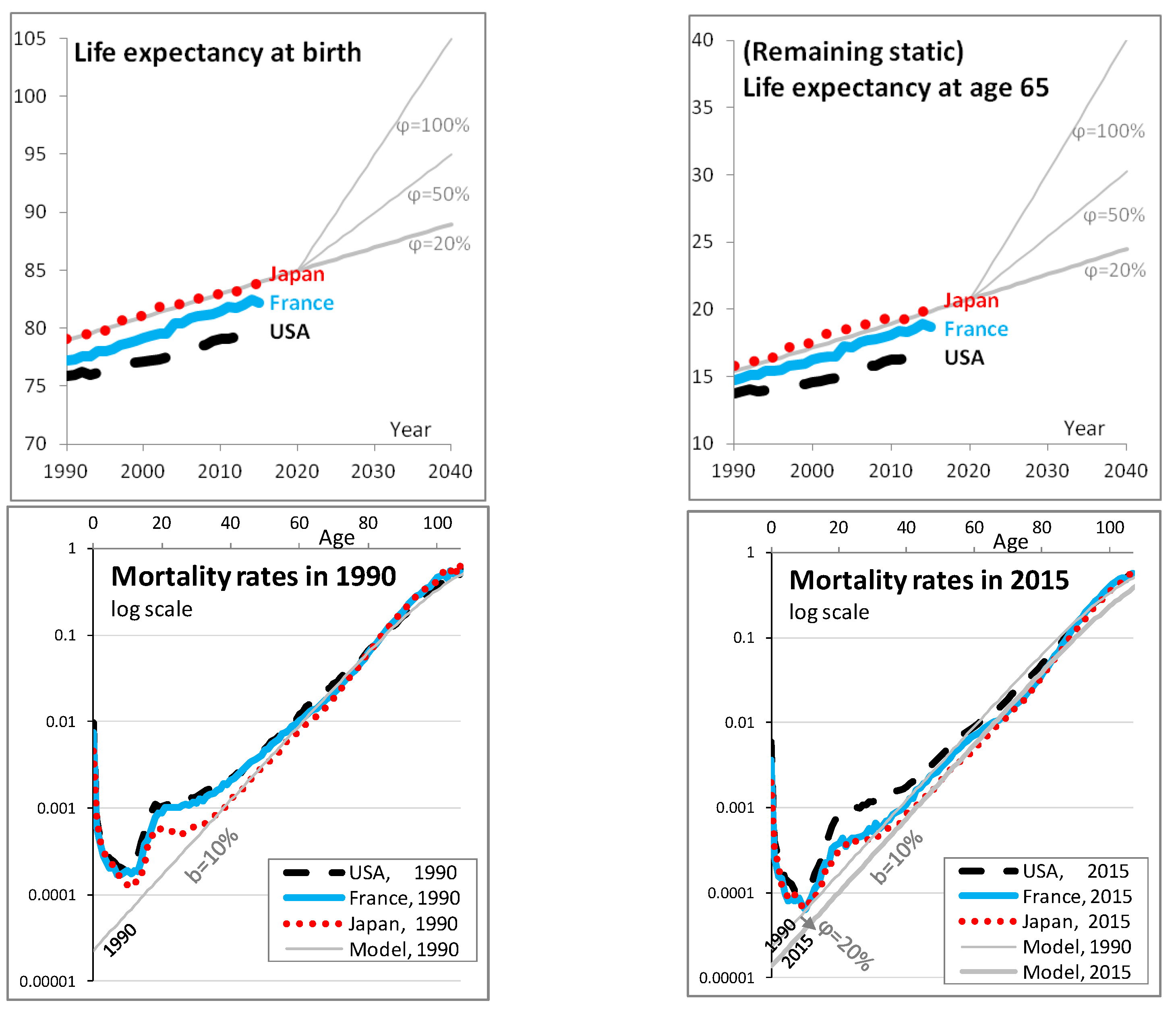
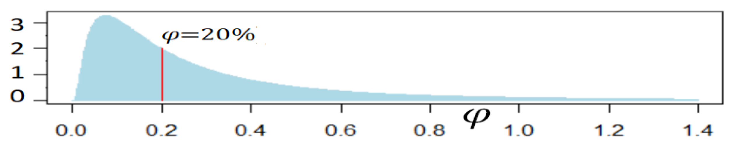
Figure 2.
Needed prudential capital depending on the future longevity trend (or lack of) expressed as a proportion of the initial wealth. In the two graphs, the y-axis shows the present value of remaining wealth after paying retirement benefits for current employees, divided by the initial wealth of the pension fund: “−1” means that 100% of additional wealth would be needed today, i.e., a needed prudential capital of the size of the initial wealth. In the first graph, the x-axis shows different scenarios for the longevity trend φ and each dot in the graph is the result of a scenario. In the second graph, the x-axis is the level at which to compute the VaR that represents the needed prudential capital: for example, a 90% VaR over all scenarios.

Figure 3.
Megafund annualized return as a function of longevity trend φ. The square represents the central scenario with a future longevity trend of 20% and an annualized return of 11.9%. If the megafund target a very wide variety of pharmaceutical developments, returns are expected to depend on the longevity trend as show by the continuous (blue lines; the thick line is the best estimate, the thin lines represent a range of uncertainty): “linkage 1”. If the megafund targets mortality-linked diseases, the expected link with longevity is the (green) dashed line.

Figure 4.
Annualized equity return, , as a function of longevity trend φ. This graph is similar as Figure 3 except that (black) curves are superimposed to should annualized equity returns: the annualized returns of investing in the equity part of the fund, rather than the whole megafund annualized return.

Figure 5.
Needed prudential capital, expressed as a proportion of the initial wealth, depending on the future longevity trend and on investments in a longevity megafund. The first graph is for a megafund that uses 50% equity investments, the second graph is for a megafund that uses 25% equity investments. Each dot in the graph is the result of a scenario of the future. In black, no investment is performed in the megafund (p1 = p2 = p3 = 0). In light gray, the pension fund invests in the longevity megafund. In gray, the pension fund invests in the generic biomedical megafund.

Table 1.
Contributions by age tranche.
| Age | Salary | Individual Annual Contribution | Annual Investment Return Rate | |
|---|---|---|---|---|
| 20 to 34 | 30,000 | 3000 | i1 = 5% | σ1 = 4% |
| 35 to 49 | 45,000 | 4500 | i2 = 4% | σ2 = 3% |
| 50 to 64 | 60,000 | 6000 | i3 = 2% | σ3 = 1% |
The table lists the assumptions used to model contributions. For example, employees from age 20 to 34 earn 30,000 each year, provide 3000 to the pension plan, this contribution has an annual return of i1,t = 5% ± 4%.
Table 2.
Needed prudential capital, expressed as a proportion of the initial wealth, depending on investments in a longevity megafund.
Table 2.
Needed prudential capital, expressed as a proportion of the initial wealth, depending on investments in a longevity megafund.
| 85% VaR | 90% VaR | 95% VaR | ||||
|---|---|---|---|---|---|---|
| No megafund | 1.4 | 2.8 | 8.5 | |||
| Longevity megafund that has 25% equity | 0.3 | 0.6 | 0.6 | 1.4 | 2.4 | 4.6 |
| Biomedical megafund that has 25% equity | 0.1 | 0.6 | 0.5 | 1.4 | 3.3 | 5.1 |
| Longevity megafund that has 50% equity | 0.3 | 0.8 | 0.9 | 1.6 | 3.1 | 4.9 |
| Biomedical megafund that has 50% equity | 0.3 | 0.7 | 0.9 | 1.6 | 4.0 | 5.8 |
| Longevity megafund that has 100% equity | 0.5 | 0.9 | 1.2 | 1.8 | 3.9 | 5.4 |
| Biomedical megafund that has 100% equity | 0.5 | 0.9 | 1.2 | 1.9 | 4.6 | 6.4 |
Each line is a different way to invest contributions, and each column is a different definition of the needed prudential capital. Each cell contains two numbers (except for the first line that serves as a reference), with a precision of circa 0.1. The first number is the needed prudential capital in case of a material investment in the megafund (p2 = 15%), the second number in case of a mild investment (p2 = 7.5%). For example, taking a 90% VaR, a material investment in a megafund leads to a needed prudential capital that is less than the initial wealth instead of almost three times the initial wealth.
© 2018 by the authors. Licensee MDPI, Basel, Switzerland. This article is an open access article distributed under the terms and conditions of the Creative Commons Attribution (CC BY) license (http://creativecommons.org/licenses/by/4.0/).
Share and Cite
MDPI and ACS Style
Debonneuil, E.; Eyraud-Loisel, A.; Planchet, F. Can Pension Funds Partially Manage Longevity Risk by Investing in a Longevity Megafund? Risks 2018, 6, 67. https://doi.org/10.3390/risks6030067
AMA Style
Debonneuil E, Eyraud-Loisel A, Planchet F. Can Pension Funds Partially Manage Longevity Risk by Investing in a Longevity Megafund? Risks. 2018; 6(3):67. https://doi.org/10.3390/risks6030067
Chicago/Turabian StyleDebonneuil, Edouard, Anne Eyraud-Loisel, and Frédéric Planchet. 2018. "Can Pension Funds Partially Manage Longevity Risk by Investing in a Longevity Megafund?" Risks 6, no. 3: 67. https://doi.org/10.3390/risks6030067
Note that from the first issue of 2016, this journal uses article numbers instead of page numbers. See further details here.