Valuation of Large Variable Annuity Portfolios Using Linear Models with Interactions

Abstract

A variable annuity is a popular life insurance product that comes with financial guarantees. Using Monte Carlo simulation to value a large variable annuity portfolio is extremely time-consuming. Metamodeling approaches have been proposed in the literature to speed up the valuation process. In metamodeling, a metamodel is first fitted to a small number of variable annuity contracts and then used to predict the values of all other contracts. However, metamodels that have been investigated in the literature are sophisticated predictive models. In this paper, we investigate the use of linear regression models with interaction effects for the valuation of large variable annuity portfolios. Our numerical results show that linear regression models with interactions are able to produce accurate predictions and can be useful additions to the toolbox of metamodels that insurance companies can use to speed up the valuation of large VA portfolios.

1. Introduction

A variable annuity (VA) is a life insurance product created by insurance companies to address concerns that many people have about outliving their assets (Ledlie et al. 2008; The Geneva Association Report 2013). Under a VA contract, the policyholder makes one lump-sum or a series of purchase payments to the insurance company and in turn, the insurance company makes benefit payments to the policyholder beginning immediately or at some future date. A typical VA has two phases: the accumulation phase and the payout phase. During the accumulation phase, the policyholder builds assets for retirement by investing the money in some investment funds provided by the insurer. During the payout phase, the policyholder receives benefit payments in either a lump-sum, periodic withdrawals or an ongoing income stream. The amount of benefit payments is tied to the performance of the investment portfolio selected by the policyholder.

To protect the policyholder’s capital against market downturns, VAs are designed to include various guarantees that share some similarities with the standard options traded in exchanges (Hardy 2003). These guarantees can be divided into two broad categories: death benefits and living benefits. A guaranteed minimum death benefit (GMDB) guarantees a specified lump sum to the beneficiary upon the death of the policyholder regardless of the performance of the investment portfolio. There are several types of living benefits. Popular living benefits include the guaranteed minimum withdrawal benefit (GMWB), the guaranteed minimum income benefit (GMIB), the guaranteed minimum maturity benefit (GMMB), and the guaranteed minimum accumulation benefit (GMAB). A GMWB guarantees that the policyholder can make systematic annual withdrawals of a specified amount from the benefit base over a period of time, even though the investment portfolio might be depleted. A GMIB guarantees that the policyholder can convert the greater of the actual account value or the benefit base to an annuity according to a specified rate. A GMMB guarantees the policyholder a specific amount at the maturity of the contract. A GMAB guarantees that the policyholder can renew the contract during a specified window after a specified waiting period, which is usually 10 years (Brown et al. 2002).

Due to the attractive guarantee features, lots of VA contracts have been sold in the past two decades. Figure 1 shows the annual VA sales in the US from 2008 to 2017. From the figure, we see that although the VA sales started declining in 2011, the annual sales in the most recent two years was still around $100 billion. Since the guarantees embedded in VAs are financial guarantees that cannot be adequately addressed by traditional actuarial methods (Boyle and Hardy 1997), having a large block of VA business creates significant financial risks for the insurance company. If the stock market goes down, for example, the insurance company loses money on all the VA contracts. Dynamic hedging is adopted by many insurance companies now to mitigate the financial risks associated with the guarantees.

Using dynamic hedging to mitigate the financial risks associated with VA guarantees, insurance companies first have to quantify the risks. This usually requires calculating the fair market values of the guarantees for a large portfolio of VA contracts in a timely manner. Since the guarantees embedded in VAs are relatively complex, their fair market values cannot be calculated in closed form. In practice, insurance companies rely on Monte Carlo simulation to calculate the fair market values of the guarantees. However, using Monte Carlo simulation to value a large portfolio of variable annuity contracts is extremely time-consuming because every contract needs to be projected over many scenarios for a long time horizon (Dardis 2016).

For example, Gan and Valdez (2017b) developed a Monte Carlo simulation model to calculate the fair market values for a portfolio of 190,000 synthetic VA contracts with 1000 risk-neutral scenarios and a 30-year projection horizon with monthly steps. The total number of cash flow projections for this portfolio is:

$$1000\times 12\times 30\times 190,000=6.84\times {10}^{10},$$

which is a huge number. As reported in Gan and Valdez (2017b), it took a single central processing unit (CPU) about 108.31 h to calculate the fair market values of the portfolio at 27 different market conditions. In other words, it took a single CPU about 4 h to calculate the fair market values for all the contracts at a single market condition. This is a great computational challenge, especially considering the complexity of the guarantees in variable annuity contracts sold in the real world.

Recently, metamodeling approaches have been proposed to address the aforementioned computational problem. See, for example, Gan (2013); Gan and Lin (2015); Gan (2015); Hejazi and Jackson (2016); Gan and Valdez (2016); Gan and Valdez (2017a); Gan and Lin (2017); Hejazi et al. (2017); Gan and Huang (2017); Xu et al. (2018); and Gan and Valdez (2018). In metamodeling, a metamodel, which is a model of the Monte Carlo simulation model, is built to replace the Monte Carlo simulation model to value the VA contracts in a large portfolio. Using metamodeling approaches can reduce significantly the runtime of valuing a large portfolio of VA contracts for the following reasons:

• Building a metamodel only requires using the Monte Carlo simulation model to value a small number of representative VA contracts.
• The metamodel is usually much simpler and faster than the Monte Carlo simulation model.

The metamodels (e.g., kriging, GB2 regression, and neural networks mentioned in Section 3) investigated in the aforementioned papers are sophisticated predictive models, which might cause difficulties in terms of interpretation or calibration. For example, fitting the GB2 regression model to the data is quite challenging (Gan and Valdez 2018). In this paper, we explore the use of linear models with interaction effects for the valuation of large VA portfolios. Unlike these existing metamodels, lines models have the advantages that they are well-known, can be fitted to data easily, and can be interpreted straightforwardly. Including the interaction effects between the features (e.g., gender, product type, account values) of VA contracts can improve the performance of linear models.

This paper is structured as follows. In Section 2, we give a description of the data we use to demonstrate the usefulness of modeling interactions for VA valuation. In Section 3, we provide a review of existing metamodeling approaches. In Section 4, we introduce the group-lasso and the overlapped group-lasso briefly. In Section 5, we present some numerical results. Finally, Section 6 concludes the paper with some remarks.

2. Description of the Data

To demonstrate the benefit of including interactions in regression models, we use a synthetic dataset obtained from Gan and Valdez (2017b). This dataset contains 190,000 VA policies, each of which is described by 45 features or variables. Since some of the variables have identical values, we exclude these variables from the regression analysis. The explanatory variables used to build regression models are described in

Table 1. Variables of VA contracts.

Variable	Description
gender	Gender of the policyholder
productType	Product type of the VA contract
gmwbBalance	GMWB balance
gbAmt	Guaranteed benefit amount
FundValuei	Account value of the ith fund, for $i=1,2,\dots ,10$
age	Age of the policyholder
ttm	Time to maturity in years

. Among these variables, gender and productType are the only categorical variables.

There are 19 types of VA contracts in the dataset. There are an equal number of VA contracts in each type, that is, there are 10,000 VA contracts of each type. For each type of VA contract, about 40% of the policyholders are female. Overall, 76,007 VA contractholders are female and 113,993 are male.

Table 2. Summary statistics of the continuous explanatory variables and the response variable.

Variable	Min	1st Q	Median	3rd Q	Max
gmwbBalance	0.00	0.00	0.00	0.00	499,708.73
gbAmt	0.00	186,864.95	316,225.98	445,940.63	1,105,731.57
FundValue1	0.00	0.00	12,635.17	49,764.15	1,099,204.71
FundValue2	0.00	0.00	15,107.17	56,882.55	1,136,895.87
FundValue3	0.00	0.00	10,043.96	39,199.69	752,945.34
FundValue4	0.00	0.00	10,383.79	39,519.79	610,579.68
FundValue5	0.00	0.00	9221.26	35,023.00	498,479.36
FundValue6	0.00	0.00	13,881.41	52,981.06	1,091,155.87
FundValue7	0.00	0.00	11,541.47	44,465.70	834,253.63
FundValue8	0.00	0.00	11,931.41	45,681.16	725,744.64
FundValue9	0.00	0.00	11,562.79	44,302.35	927,513.49
FundValue10	0.00	0.00	11,850.05	44,967.78	785,978.60
age	34.52	42.03	49.45	56.96	64.46
ttm	0.59	10.34	14.51	18.76	28.52
fmv	−94,944.17	−5142.94	12,488.63	66,814.16	1,536,700.08

shows some summary statistics of the continuous explanatory variables and the response variable, which is the fair market value. From the table, we see that most of the contracts have zero gmwbBalance because most of the contracts do not include a GMWB. For every investment fund, many contracts have zero account values because many policyholders did not invest in the fund. The maturity of the contracts ranges from less than 1 year to about 29 years.

Table 2 also shows the summary statistics of the fair market value, which is the response variable. The fair market value is calculated as the difference between the benefit and the risk charge. When the benefit is less than the risk charge, the fair market value is negative; otherwise, the fair market value is positive. Figure 2 shows a histogram of the fair market values. From the figure, we see that most of the fair market values are positive and the distribution is positively skewed. Regarding the runtime used by the Monte Carlo simulation to calculate these fair market values, it was about 108 h if a single CPU was used. See Gan and Valdez (2017b) for details.

3. Existing Metamodeling Approaches

In this section, we give a review of some existing metamodeling approaches. A metamodeling approach involves the following four major steps:

• select a small number of representative VA contracts (i.e., experimental design).
• use Monte Carlo simulation to calculate the fair market values (or other quantities of interest) of the representative contracts.
• build a regression model (i.e., the metamodel) based on the representative contracts and their fair market values.
• use the regression model to estimate the fair market value for every VA contract in the portfolio.

From the above steps, we see that the main idea of metamodeling is to build a predictive model based on a small number of representative VA contracts in order to reduce the number of contracts that are valued by Monte Carlo simulation.

Table 3. Some publications on metamodeling approaches.

Publication	Experimental Design	Metamodel
Gan (2013)	Clustering	Kriging
Gan and Lin (2015)	Clustering	Kriging
Gan (2015)	LHS	Kriging
Hejazi and Jackson (2016)	Uniform sampling	Neural network
Gan and Valdez (2016)	Clustering, LHS	GB2 regression
Gan and Valdez (2017a)	Clustering	Gamma regression
Gan and Lin (2017)	LHS, conditional LHS	Kriging
Hejazi et al. (2017)	Uniform sampling	Kriging, IDW, RBF
Gan and Huang (2017)	Clustering	Kriging
Xu et al. (2018)	Random sampling	Neural network, regression trees
Gan and Valdez (2018)	Clustering	GB2 regression

lists some papers related to metamodeling approaches for the valuation of large VA portfolios. The paper by Gan (2013) is perhaps the first paper published in academic journals that studies the use of metamodeling for the valuation of large VA portfolios. In Gan (2013), the k-prototype algorithm, which is a clustering algorithm proposed by Huang (1998), was used to select representative VA contracts and the ordinary kriging was used as the metamodel. The dataset used in Gan (2013) is much simpler than the dataset described in Section 2. Gan and Lin (2015) studied the use of metamodeling for the valuation of large VA portfolios under the stochastic-on-stochastic simulation framework. In Gan and Lin (2015), the k-prototype algorithm was used to select representative VA contracts and the universal kriging for functional data (UKFD) was used as the metamodel.

Since the k-prototype algorithm is not efficient for selecting a moderate number (e.g., 200) of representative VA contracts, Gan (2015) studied the use of Latin hypercube sampling (LHS) for selecting representative contracts. Gan and Huang (2017) used the truncated fuzzy c-means (TFMC) algorithm, which is a scalable clustering algorithm developed by Gan et al. (2016), to select representative contracts. Further, Gan and Valdez (2016) investigated several methods for selecting representative VA contracts and found that the clustering method and the LHS method are comparable in accuracy and are better than other methods such as random sampling. The LHS and the conditional LHS methods are also used in Gan and Lin (2017), which studied the use of metamodeling to calculate dollar deltas quickly for daily hedging purpose.

Hejazi and Jackson (2016) studied the use of neural networks for the valuation of large VA portfolio. The dataset used in their study is similar to the one used in Gan (2013). Xu et al. (2018) proposed neural networks as well as tree-based models with moment matching to value large VA portfolios. Hejazi et al. (2017) treated the valuation of large VA portfolios as a spatial interpolation problem and investigated several interpolation methods, including the inverse distance weighting (IDW) method and the radial basis function (RBF) method.

Gan and Valdez (2017a) investigated the use of copula to model the dependency of partial dollar deltas. They found that the use of copula does not improve the prediction accuracy of the metamodel because the dependency is well captured by the covariates. To address the skewness typically observed in the distribution of the fair market values, Gan and Valdez (2018) proposed the use of the generalized beta of the second kind (GB2) distribution to model the fair market values. Gan and Huang (2017) proposed a data mining framework for the valuation of large VA portfolios.

In all the work mentioned above, the interactions between the variables are not considered in the metamodels. In addition, some of the metamodels (e.g., kriging, neural networks, GB2 regression) are quite sophisticated. Fitting such metamodels poses challenges. As reported in Gan and Valdez (2018), for example, fitting GB2 regression models to the VA data is not straightforward and requires a multi-stage optimization procedure.

4. Learning Interactions

Jaccard and Turrisi (2003) discussed six basic types of relationships that can occur in a causal model, which specifies the effects of one or more independent variables on one or more dependent variables. These causal relationships are illustrated in

Table 4. Six basic types of causal relationships.

Relationship	Example
Direct causal relationship
Indirect causal relationship
Spurious relationship
Bidirectional causal relationship
Unanalyzed relationship
Moderated causal relationship

. A direct causal relationship occurs between two variables X and Y when X is a direct cause of Y, that is, X is the immediate determinant of Y. An indirect causal relationship occurs between X and Y when X exerts a causal impact on Y but only through its impact on a third variable Z. A bidirectional or reciprocal causal relationship occurs between X and Y when X has a causal impact on Y and Y has a causal impact on X. A causal relationship is called an unanalyzed relationship when X and Y are related but the source of the relationship is unspecified. A moderated causal relationship occurs when the relationship between X and Y is moderated by a third variable Z.

Moderated relationships are often called interaction effects (Cox 1984; Jaccard and Turrisi 2003). Interaction effects are most commonly considered in the context of regression analysis. An interaction occurs between two independent variables when the effect of one independent variable on the dependent variable changes depending on the level of another independent variable. Mathematically, consider the following function:

$$Y=f(X,Z),$$

(1)

where X and Z are independent variables and Y is a dependent variable. An interaction exists between X and Z in f if f cannot be expressed as $g\left(X\right)+h\left(Z\right)$ for any functions g and h. In other words, interactions exist when the response cannot be explained by additive functions of the independent variables. The literature related to modeling interactions in actuarial science is scarce. In the master thesis, Nawar (2016) investigated learning pairwise interactions in the Poisson and Gamma regression models for P&C insurance.

Let Y be a continuous response variable. Let $X_1$, $X_2$, …, $X_p$ be p explanatory variables, which include continuous and categorical variables. The the first-order interaction model is given by (Lim and Hastie 2015):

$$E\left[Y\right|X_1,X_2,\dots ,X_p]={\beta }_0+{\displaystyle \sum _{j=1}^p}{\beta }_j{X}_j+{\displaystyle \sum _{s<t}}{\beta }_{s:t}{X}_{s:t},$$

(2)

where the term $X_{s:t}=X_s{X}_t$ denotes the interaction effect between $X_s$ and $X_t$ and terms $X_1$, $X_2$, …, $X_p$ denote the main effects. The interaction model is said to satisfy strong hierarchy if an interaction can exist only if both its main effects are present. The interaction model is said to satisfy weak hierarchy if an interaction can exist as long as either of its main effects is present. Main effects can be viewed as deviations from the global mean and interaction effects can be viewed as deviations from the main effects. As a result, it rarely makes sense to have interactions without main effects. This means that hierarchical interaction models are usually preferred.

From Equation (2), we see that the first-order interaction model is an extension of the multiple linear regression model by adding some interaction terms. One major advantage of adding the interaction terms is that it helps increase the predictive power.

However, learning interactions is a challenging problem, especially when there are many variables. For example, the number of pairwise interaction terms among 20 variables is $20\times 19/2=190$, which may exceed the number of training samples. If we include all the pairwise interaction terms in the regression model, then the resulting model may overfit the data. To avoid the overfitting problem, we need to select important interactions only. However, selecting important interactions from a large number of interactions manually is a tedious task.

To address the aforementioned challenges, we use the overlapped group-lasso proposed by Lim and Hastie (2015) that can produce hierarchical interaction models automatically. The overlapped group-lasso is based on the group-lasso proposed by Yuan and Lin (2006) by adding an overlapped group-lasso penalty. In the following subsections, we give a brief introduction of the group-lasso and the overlapped group-lasso.

4.1. Group-Lasso

The group-lasso can be viewed as a general version of the popular lasso proposed by Tibshirani (1996). Let $\mathbf{y}={(y_1,y_2,\dots ,y_n)}^{\prime }$ denote the vector of responses and let $\mathbf{X}$ denote the design matrix. Then the lasso is defined as

$${\widehat{\mathit{\beta }}}^{LASSO}=arg\underset{\mathit{\beta }}{min}\left(\frac{1}{2}{\parallel \mathbf{y}-\mathbf{X}\mathit{\beta }\parallel }_2^2+\lambda {\parallel \mathit{\beta }\parallel }_1\right),$$

(3)

where ${\parallel ·\parallel }_2$ denotes the ${\ell }^2$-norm, ${\parallel ·\parallel }_1$ denotes the ${\ell }^1$-norm, and $\lambda$ is a tuning parameter that controls the amount of regularization. The ${\ell }^1$-norm induces sparsity in the solution in the sense that it sets some coefficients to zero. A larger value of $\lambda$ implies more regularization. The lasso solution is piecewise linear with respect to the tuning parameter $\lambda$. The least angle regression selection (LARS) (Efron et al. 2004) is an efficient algorithm to solve the optimization problem in Equation (3) for all $\lambda \in [0,\infty ]$. The final value of $\lambda$ can be selected by techniques such as cross-validation.

The lasso is designed for selecting individual input variables but not for general factor selection. Yuan and Lin (2006) proposed group-lasso that aims to select important factors. Suppose that there are p groups of variables. For $j=1,2,\dots ,p$, let ${\mathbf{X}}_j$ denote the feature matrix for group j. The group-lasso can be formulated as follows:

$${\widehat{\mathit{\beta }}}^{GLASSO}=arg\underset{\mathit{\beta }}{min}\left(\frac{1}{2}{\parallel \mathbf{y}-{\beta }_0\mathbf{1}-{\displaystyle \sum _{j=1}^p}{\mathbf{X}}_j{\mathit{\beta }}_j\parallel }_2^2+\lambda {\displaystyle \sum _{j=1}^p}{\gamma }_j{\parallel {\mathit{\beta }}_j\parallel }_2\right),$$

(4)

where $\mathbf{1}$ is a vector of ones, ${\parallel ·\parallel }_2$ denotes the ${\ell }^2$-norm, and $\lambda ,{\gamma }_1,\dots ,{\gamma }_p$ are tuning parameters. The parameter $\lambda$ controls the overall amount of regularization while the parameters ${\gamma }_1,\dots ,{\gamma }_p$ allow each group to be penalized to different extents. When each group contains one continuous variable, the group-lasso reduces to the lasso. Like the lasso, the penalty on coefficients will force some ${\widehat{\mathit{\beta }}}_j$ to be zero. An attractive property of the group-lasso is that if ${\widehat{\mathit{\beta }}}_j$ is nonzero, then all its components are typically nonzero.

The optimization problem in Equation (4) can be solved by starting with a value of $\lambda$ that is just large enough to make all estimates zero. Then a path of solutions can be obtained by decreasing $\lambda$ along a grid of values. An optimal $\lambda$ can be chosen by cross-validation.

4.2. Overlapped Group-Lasso

The overlapped group-lasso extends the group-lasso by adding an overlapped group-lasso penalty to the loss function in order to obtain hierarchical interaction models. The overlapped group-lasso is formulated as the following constrained optimization problem (Lim and Hastie 2015):

$$\begin{array}{ccc}\hfill {\widehat{\mathit{\beta }}}^{OGLASSO}& \hfill =& arg\underset{\mathit{\beta }}{min}\left(\frac{1}{2}{∥\mathbf{y}-{\beta }_0\mathbf{1}-{\sum }_{j=1}^p{\mathbf{X}}_j{\mathit{\beta }}_j-{\sum }_{s<t}({\mathbf{X}}_s{\tilde{\mathit{\beta }}}_s+{\mathbf{X}}_t{\tilde{\mathit{\beta }}}_t+{\mathbf{X}}_{s:t}{\mathit{\beta }}_{s:t})∥}_2^2\right.\hfill \\ & & \left.+\lambda \left({\sum }_{j=1}^p{\parallel {\mathit{\beta }}_j\parallel }_2+{\sum }_{s<t}\sqrt{L_s{\parallel {\tilde{\mathit{\beta }}}_s\parallel }_2^2+L_t{\parallel {\tilde{\mathit{\beta }}}_t\parallel }_2^2+{\parallel {\mathit{\beta }}_{s:t}\parallel }_2^2}\right)\right),\hfill \end{array}$$

(5)

subject to the following sets of constraints:

$$\left\{\begin{array}{cc}{\sum }_{l=1}^{m_j}{\beta }_j^{\left(l\right)}=0,{\sum }_{l=1}^{m_j}{\tilde{\beta }}_j^{\left(l\right)}=0,\hfill & \mathrm{if}{X}_j\mathrm{is}\mathrm{categorical};\hfill \\ {\sum }_{l=1}^{m_j}{\beta }_{t:j}^{\left(l\right)}=0,\hfill & \mathrm{if}{X}_j\mathrm{is}\mathrm{categorical}\mathrm{and}{X}_t\mathrm{is}\mathrm{continuous};\hfill \\ {\sum }_{l=1}^{m_j}{\beta }_{t:j}^{(l,k)}=0\forall k,{\sum }_{k=1}^{m_t}{\beta }_{t:j}^{(l,k)}=0\forall l,\hfill & \mathrm{if}{X}_j\mathrm{and}{X}_t\mathrm{are}\mathrm{categorical},\hfill \end{array}\right.$$

(6)

where $m_j$ is the number of levels of $X_j$, $m_t$ is the number of levels of $X_t$, ${\beta }_j^{\left(l\right)}$ is the lth entry of ${\mathit{\beta }}_j$, ${\tilde{\beta }}_j^{\left(l\right)}$ is the lth entry of ${\tilde{\mathit{\beta }}}_j$, and ${\beta }_{t:j}^{(l,k)}$ is the lkth entry of ${\mathit{\beta }}_{t:j}$. The constants $L_s$ and $L_t$ are selected such that ${\tilde{\mathit{\beta }}}_s$, ${\tilde{\mathit{\beta }}}_t$, and ${\mathit{\beta }}_{s:t}$ are on the same scale.

In Equation (5), ${\mathbf{X}}_1$, ${\mathbf{X}}_2$, …, ${\mathbf{X}}_p$ denote the feature matrices of the p group of variables, $X_1$, $X_2$, …, $X_p$, which include continuous and categorical variables. If $X_j$ is continuous, then ${\mathbf{X}}_j$ is just a one-column matrix containing the values of $X_j$, that is,

$${\mathbf{X}}_j={(x_{1j},x_{2j},\dots ,x_{nj})}^{\prime },$$

(7)

where n is the number of observations and $x_{ij}$ is the value of $X_j$ in the ith observation. If $X_j$ is categorical, then ${\mathbf{X}}_j$ contains all the dummy variables associated with $X_j$. For example, if $X_j$ has $m_j$ levels, then ${\mathbf{X}}_j$ is an $n\times m_j$ indicator matrix where the $(i,l)$-entry is 1 if the value of $X_j$ in the ith observation is equal to the lth level; otherwise, the $(i,l)$-entry is zero.

The matrix ${\mathbf{X}}_{s:t}$ denotes the feature matrix of the interaction term, which is defined as

$${\mathbf{X}}_{s:t}=\left\{\begin{array}{cc}{\mathbf{X}}_s\ast {\mathbf{X}}_t,\hfill & \mathrm{if}{X}_s\mathrm{and}{X}_t\mathrm{are}\mathrm{categorical},\hfill \\ {\mathbf{X}}_s\ast \left[\mathbf{1}{\mathbf{X}}_t\right],\hfill & \mathrm{if}{X}_s\mathrm{is}\mathrm{categorical}\mathrm{and}{X}_t\mathrm{is}\mathrm{continuous},\hfill \\ \mathbf{1}{\mathbf{X}}_s]\ast {\mathbf{X}}_t,\hfill & \mathrm{if}{X}_s\mathrm{is}\mathrm{continuous}\mathrm{and}{X}_t\mathrm{is}\mathrm{categorical},\hfill \\ \mathbf{1}{\mathbf{X}}_s]\ast \left[\mathbf{1}{\mathbf{X}}_s\right],\hfill & \mathrm{if}{X}_s\mathrm{and}{X}_t\mathrm{are}\mathrm{continuous},\hfill \end{array}\right.$$

(8)

where $\mathbf{A}\ast \mathbf{B}$ denotes a matrix consisting of all pairwise products of columns of $\mathbf{A}$ and $\mathbf{B}$. For example, for $\mathbf{A}$ and $\mathbf{B}$ given by

$$\mathbf{A}=\left(\begin{array}{cc}{a}_{11}& a_{12}\\ a_{21}& a_{22}\\ a_{31}& a_{32}\end{array}\right),\mathbf{B}=\left(\begin{array}{cc}{b}_{11}& b_{12}\\ b_{21}& b_{22}\\ b_{31}& b_{32}\end{array}\right),$$

(9)

the matrix $\mathbf{A}\ast \mathbf{B}$ is calculated as

$$\mathbf{A}\ast \mathbf{B}=\left(\begin{array}{cccc}{a}_{11}{b}_{11}& a_{11}{b}_{12}& a_{12}{b}_{11}& a_{12}{b}_{12}\\ a_{21}{b}_{21}& a_{21}{b}_{22}& a_{22}{b}_{21}& a_{22}{b}_{22}\\ a_{31}{b}_{31}& a_{31}{b}_{32}& a_{32}{b}_{31}& a_{32}{b}_{32}\end{array}\right).$$

(10)

As mentioned above, if the jth variable $X_j$ is categorical, the feature matrices ${\mathbf{X}}_j$, ${\mathbf{X}}_{1:j}$, …, ${\mathbf{X}}_{j-1:j}$ in Equation (5) contain all the dummy variables associated with $X_j$. As a result, these terms are overparameterized. That is why the corresponding coefficients vectors are constrained.

In Equation (5), we see that the main effect matrix ${\mathbf{X}}_j$ has two coefficient vectors ${\mathit{\beta }}_j$ and ${\tilde{\mathit{\beta }}}_j$. This creates an overlap in the penalties. The ultimate coefficient for ${\mathbf{X}}_j$ is the sum of the two coefficient vectors, i.e., ${\mathit{\beta }}_j+{\tilde{\mathit{\beta }}}_j$. The term $\sqrt{L_s{\parallel {\tilde{\mathit{\beta }}}_s\parallel }_2^2+L_t{\parallel {\tilde{\mathit{\beta }}}_t\parallel }_2^2+{\parallel {\mathit{\beta }}_{s:t}\parallel }_2^2}$ in Equation (5) leads to solutions that satisfy strong hierarchy in the sense that either ${\widehat{\tilde{\mathit{\beta }}}}_s={\widehat{\tilde{\mathit{\beta }}}}_t={\widehat{\mathit{\beta }}}_{s:t}=0$ or all are nonzero. In other words, if an interaction is present, then both main effects are present.

Lim and Hastie (2015) showed that the overlapped group-lasso, which is formulated as a constrained optimization problem, is equivalent to the unconstrained group-lasso. Precisely, solving the constrained optimization problem in Equation (5) is equivalent to solving the following unconstrained optimization problem:

$$\begin{array}{ccc}\hfill {\widehat{\mathit{\beta }}}^{OGLASSO}& \hfill =& arg\underset{\mathit{\beta }}{min}\left(\frac{1}{2}{∥\mathbf{y}-{\beta }_0\mathbf{1}-{\sum }_{j=1}^p{\mathbf{X}}_j{\mathit{\beta }}_j-{\sum }_{s<t}{\mathbf{X}}_{s:t}{\mathit{\beta }}_{s:t}∥}_2^2\right.\hfill \\ & & \left.+\lambda \left({\sum }_{j=1}^p{\parallel {\mathit{\beta }}_j\parallel }_2+{\sum }_{s<t}{\parallel {\mathit{\beta }}_{s:t}\parallel }_2\right)\right).\hfill \end{array}$$

(11)

Because of the equivalence, the overlapped group-lasso can be solved efficiently.

5. Numerical Results

In this section, we present some numerical results to show the usefulness of including interactions in linear regression models. In particular, we will compare the performance of the linear regression models with and without interactions.

5.1. Experimental Setup

As mentioned in Section 3, metamodeling has two major components: an experimental design method and a metamodel. The experimental design method is used to select representative VA contracts. The metamodel is first fitted to the representative VA contracts and then used to predict the fair market values of all the VA contracts in the portfolio.

Since this paper focuses on metamodels that include and do not include interactions, we just use random sampling as the experimental design method to minimize the effect of experimental design on the accuracy of the metamodel.

Another important factor to consider in metamodeling is the number of representative VA contracts. There is a trade-off between accuracy and speed. If only a few representative VA contracts are used, then it takes less time to run Monte Carlo valuation for the representative VA contracts. However, the fitted metamodel might not be accurate. If a lot of representative VA contracts are used, then the fitted metamodel performs well in terms of prediction accuracy. However, in this case it takes more time to run Monte Carlo simulation. In this paper, we follow the strategy used in previous studies (e.g., Gan and Lin 2015) to determine the number of representative VA contracts, that is, we use 10 times the number of predictors, including the dummy variables converted from categorical variables. Since there are 34 predictors, we start with 340 representative VA contracts. We also use 680 representative VA contracts to see the impact of the number of representative VA contracts on the performance of the metamodels.

To fit linear models to the data, we use the R function lm from the stats package. To fit the overlapped group-lasso, we use the R function glinternet.cv with default settings from the glinternet package developed by Lim and Hastie (2018). We use 10-fold cross-validation to select the best value of $\lambda$ in Equation (5).

5.2. Validation Measures

To compare the prediction accuracy of the metamodels, we use the following three validation measures: the percentage error at the portfolio level, the $R^2$ (Frees 2009), and the concordance correlation coefficient (Lin 1989).

Let $y_i$ denote the fair market value of the ith VA policy in the portfolio that is calculated by Monte Carlo simulation method. Let ${\widehat{y}}_i$ denote the fair market value predicted by a metamodel. Then the percentage error ($PE$) at the portfolio level is defined as

$$PE={\displaystyle \frac{{\displaystyle \sum _{i=1}^n}(y_i-{\widehat{y}}_i)}{{\displaystyle \sum _{i=1}^n}{y}_i}},$$

(12)

where n is the number of VA policies in the portfolio. Between two metamodels, the one producing a PE that is closer to zero is better.

The $R^2$ is calculated as

$$R^2=1-{\displaystyle \frac{{\displaystyle \sum _{i=1}^n}{(y_i-{\widehat{y}}_i)}^2}{{\displaystyle \sum _{i=1}^n}{(y_i-\overline{y})}^2}},$$

(13)

where $\overline{y}$ is the average of $y_1,y_2,\dots ,y_n$. Between two metamodels, the one that produces a lower MSE is better.

The concordance correlation coefficient ($CCC$) is used to measure the agreement between two variables. It is defined as follows (Lin 1989):

$$CCC={\displaystyle \frac{2\rho {\sigma }_1{\sigma }_2}{{\sigma }_1^2+{\sigma }_2^2+{({\mu }_1-{\mu }_2)}^2}}.$$

(14)

where $\rho$ is the correlation between $(y_1,y_2,\dots ,y_n)$ and $({\widehat{y}}_1,{\widehat{y}}_2,\dots ,{\widehat{y}}_n)$, ${\sigma }_1$ and ${\mu }_1$ are the standard deviation and the mean of $(y_1,y_2,\dots ,y_n)$, respectively, and ${\sigma }_2$ and ${\mu }_2$ are the standard deviation and the mean of $({\widehat{y}}_1$, ${\widehat{y}}_2$, …, ${\widehat{y}}_n)$, respectively. Between two metamodels, the one that produces a higher CCC is considered a better model. In particular, a value of 1 indicates perfect agreement between the two models.

5.3. Results

To demonstrate the benefit of including interactions in regression models, we fitted a multiple linear regression model without interactions and the first-order interaction model defined in Equation (2) to the representative VA contracts. We conducted our experiments on a Laptop computer with a Windows operating system and 8 GB memory.

Table 5. Accuracy and runtime of the metamodels when 340 representative VA contracts were used. The runtime is in seconds.

Model	PE	R2	CCC	Runtime
Linear Model without interactions	0.0207	0.7986	0.8957	0.2700
Linear Model with interactions	−0.0036	0.9441	0.9697	37.8900

shows the values of the validation measures for the linear models with and without interactions when 340 representative VA contracts were used. All the validation measures show that the linear model with interactions outperformed the one without interactions in terms of accuracy. At the portfolio level, for example, the percentage error of the linear model with interactions is around −0.4%, while the percentage error of the linear model without interactions is around 2.1%, which is higher. Since we used 10-fold cross validation to select the optimal tuning parameter $\lambda$ in the overlapped group-lasso, the runtime used to fit the linear model with interactions is higher.

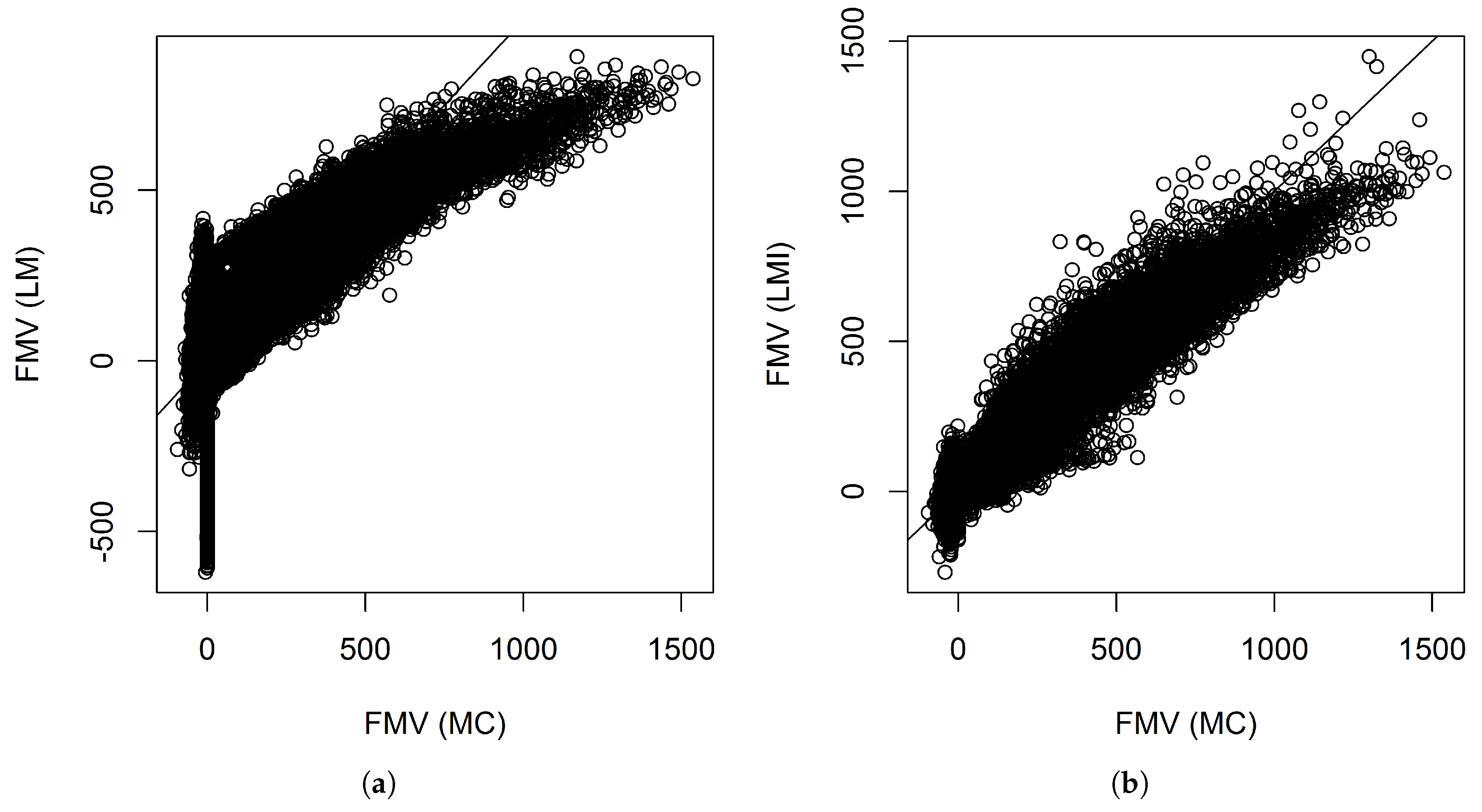
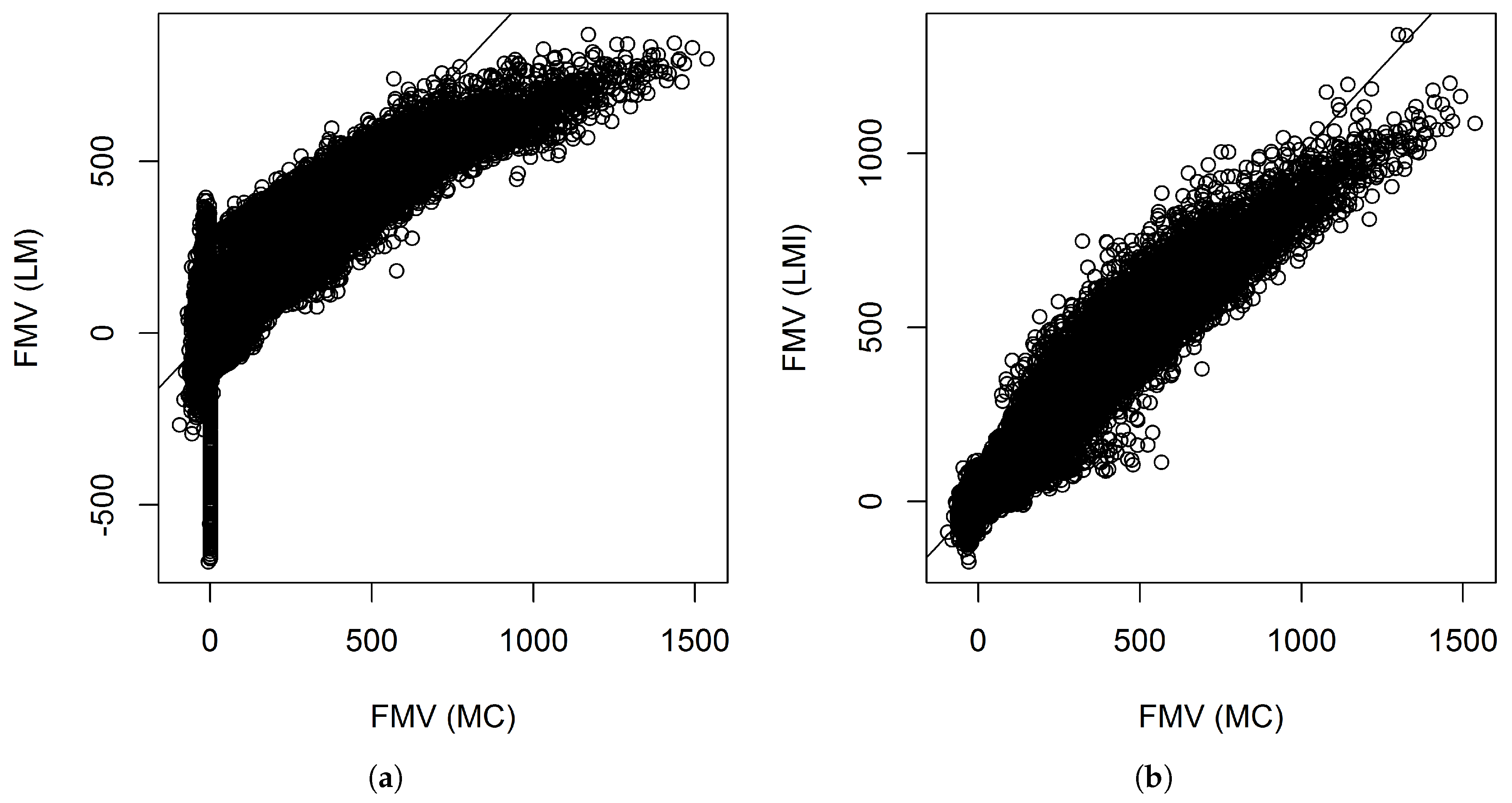
Figure 3 shows the scatter plots between the fair market values calculated by Monte Carlo and those predicted by the linear models with and without interactions when 340 representative VA contracts were used. The figures show that the linear model without interactions did not fit the tails well. For example, many of the contracts have near zero fair market values. However, their fair market values predicted by the linear model without interactions ranges from less than −$500 thousand to near $500 thousand.

Table 6. Summary statistics of the prediction errors of individual VA contracts when 340 representative VA contracts were used.

Model	Min	1st Q	Median	Mean	3rd Q	Max
Linear Model without interactions	−432.13	−28.46	1.08	−1.40	25.97	708.65
Linear Model with interactions	−515.96	−12.23	−2.25	0.10	7.57	478.52

shows some summary statistics of the prediction errors of individual VA contracts. From the table, we see that prediction errors of the linear model with interactions have a more symmetric distribution.

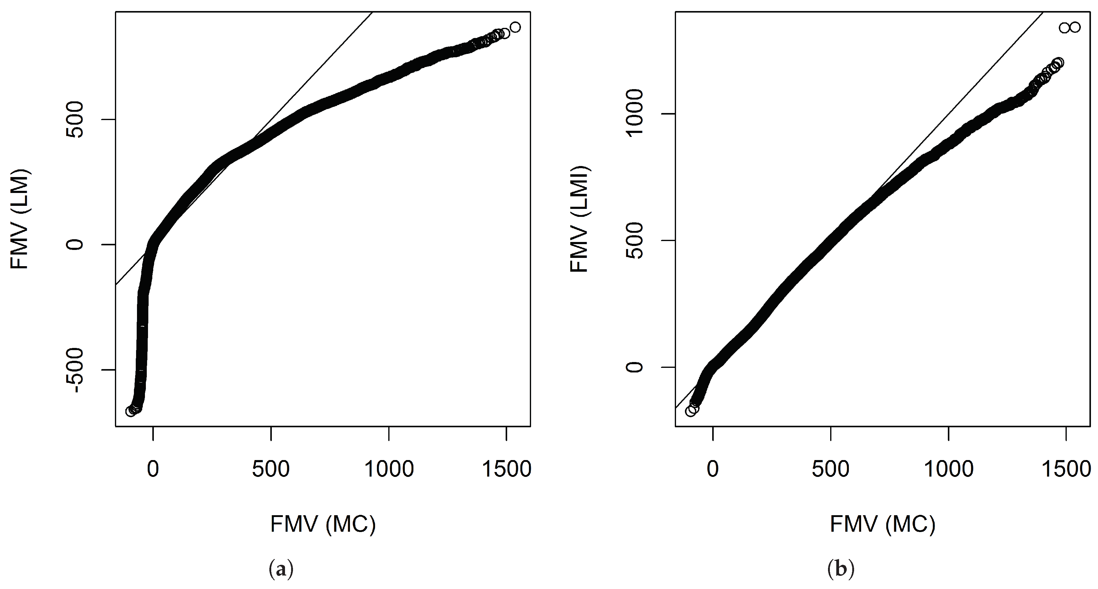
Figure 4 shows the QQ plots produced by the linear model with interactions found by the overlapped group-lasso and the linear model without interactions. If we look at these plots, we see that the linear model with interactions worked pretty well, although the fitting at the tails is a little bit off.

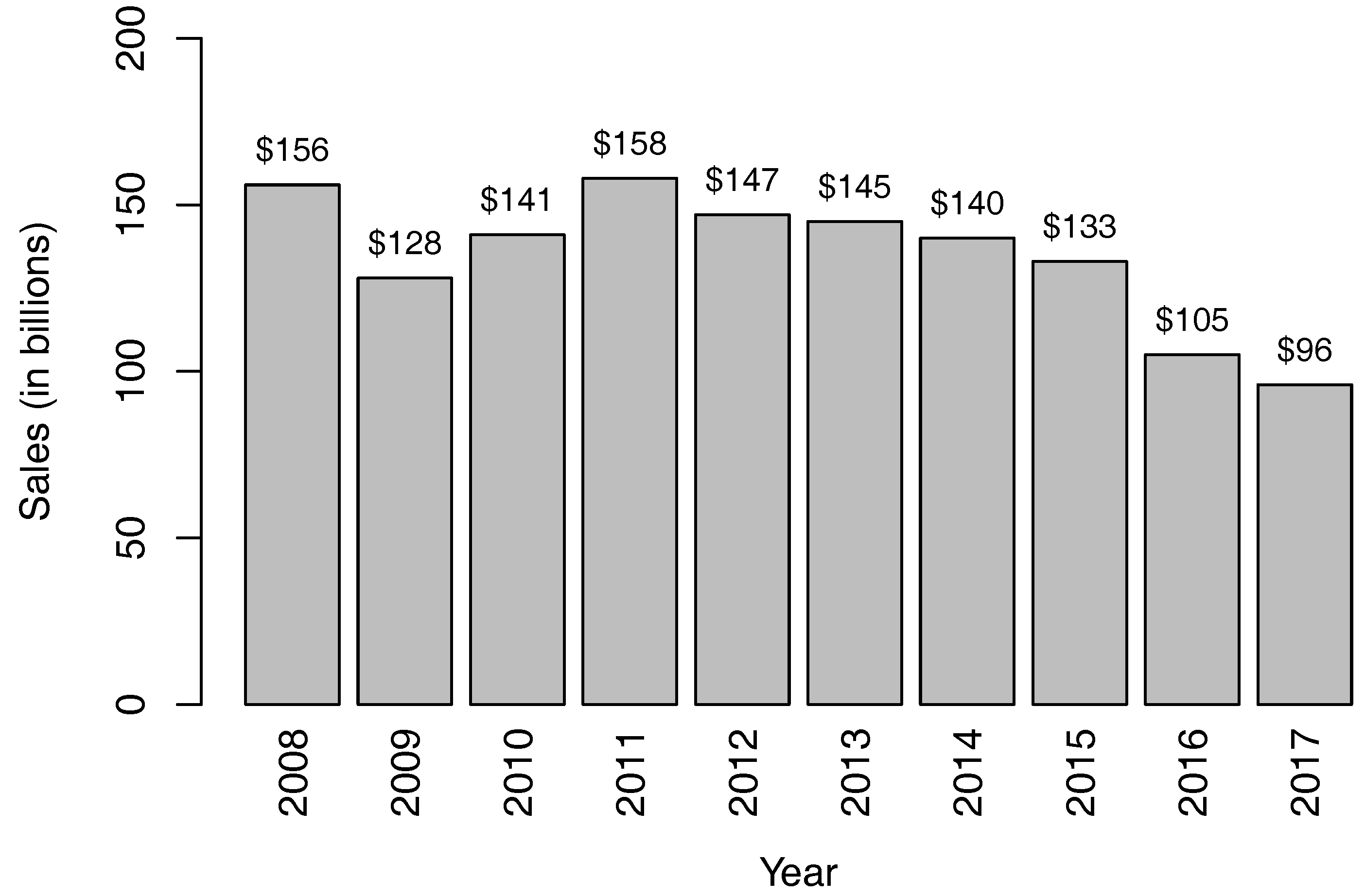
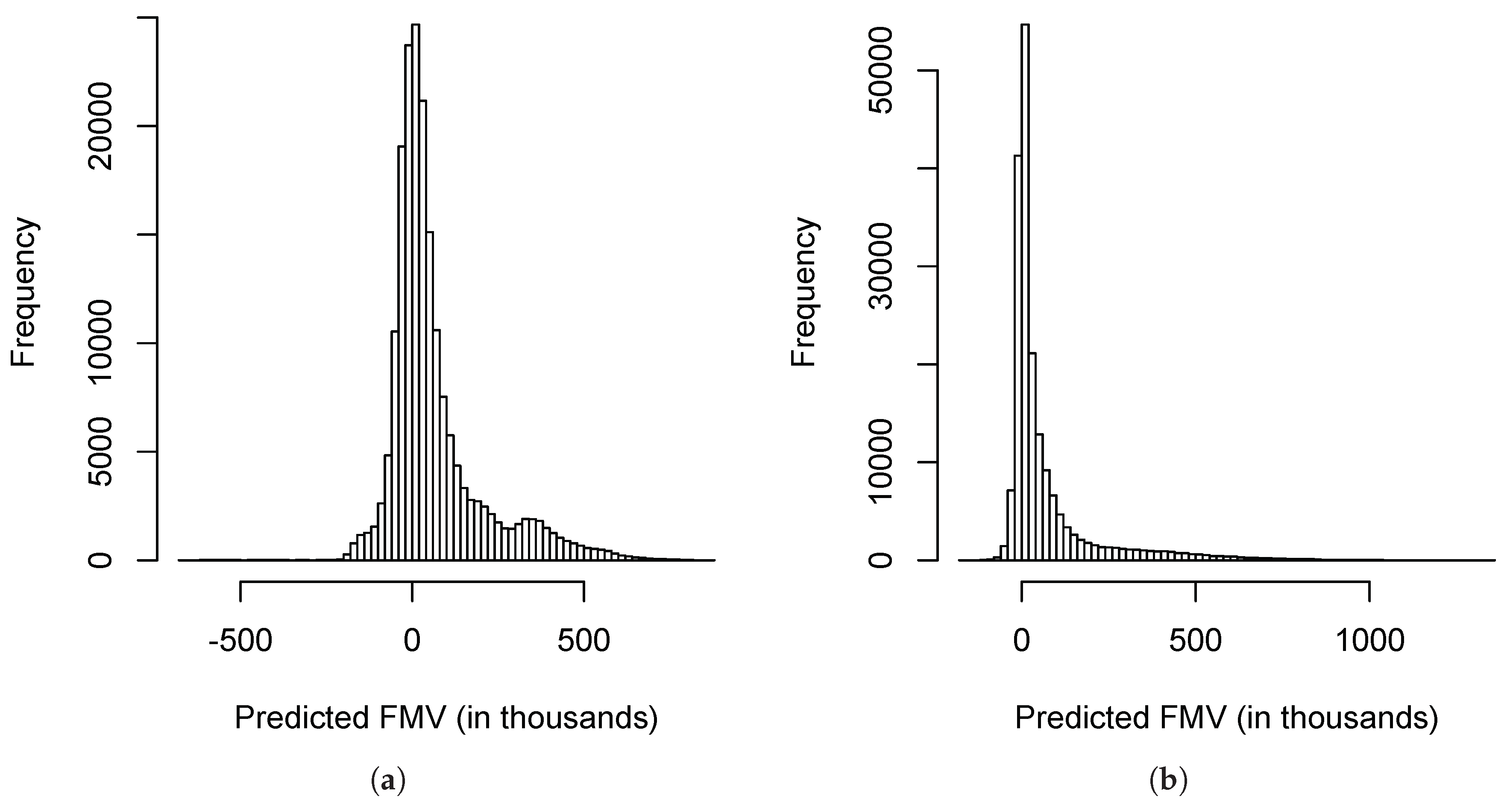
Figure 5 shows the histograms of the fair market values predicted by the linear models with and without interactions. Between the two histograms, the histogram produced by the linear model with interactions is more similar to the histogram of the data shown in Figure 2.

If we compare Figure 3b, Figure 4b and Figure 5b to Figure 3a, Figure 4a and Figure 5a, we can see that the improvement that resulted from including interactions is significant.

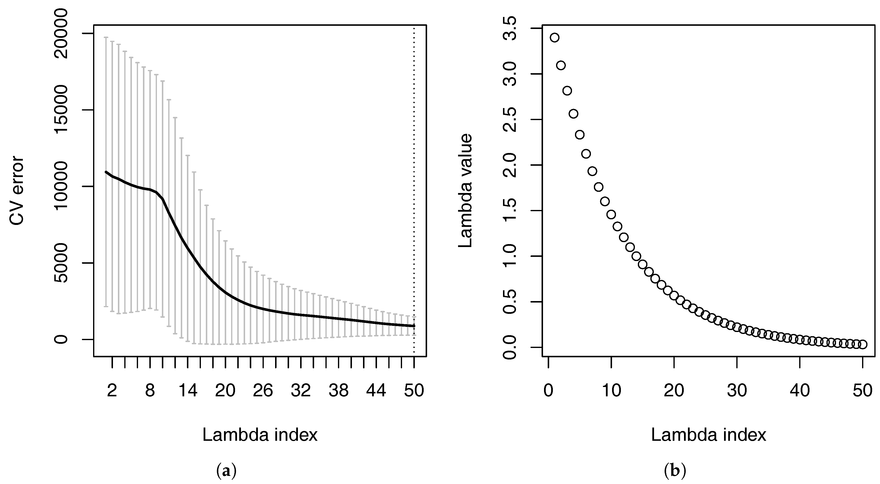
Figure 6a shows the cross-validation errors of the linear model with interactions at different values of the tuning parameter $\lambda$. Figure 6b shows the these values of $\lambda$. When the value of $\lambda$ is large, many of the coefficients are forced to be zero because of the penalty. When many of the coefficients are zero, the linear model with interactions produces large cross-validation errors. When the value of $\lambda$ decreases, the cross-validation error also decreases.

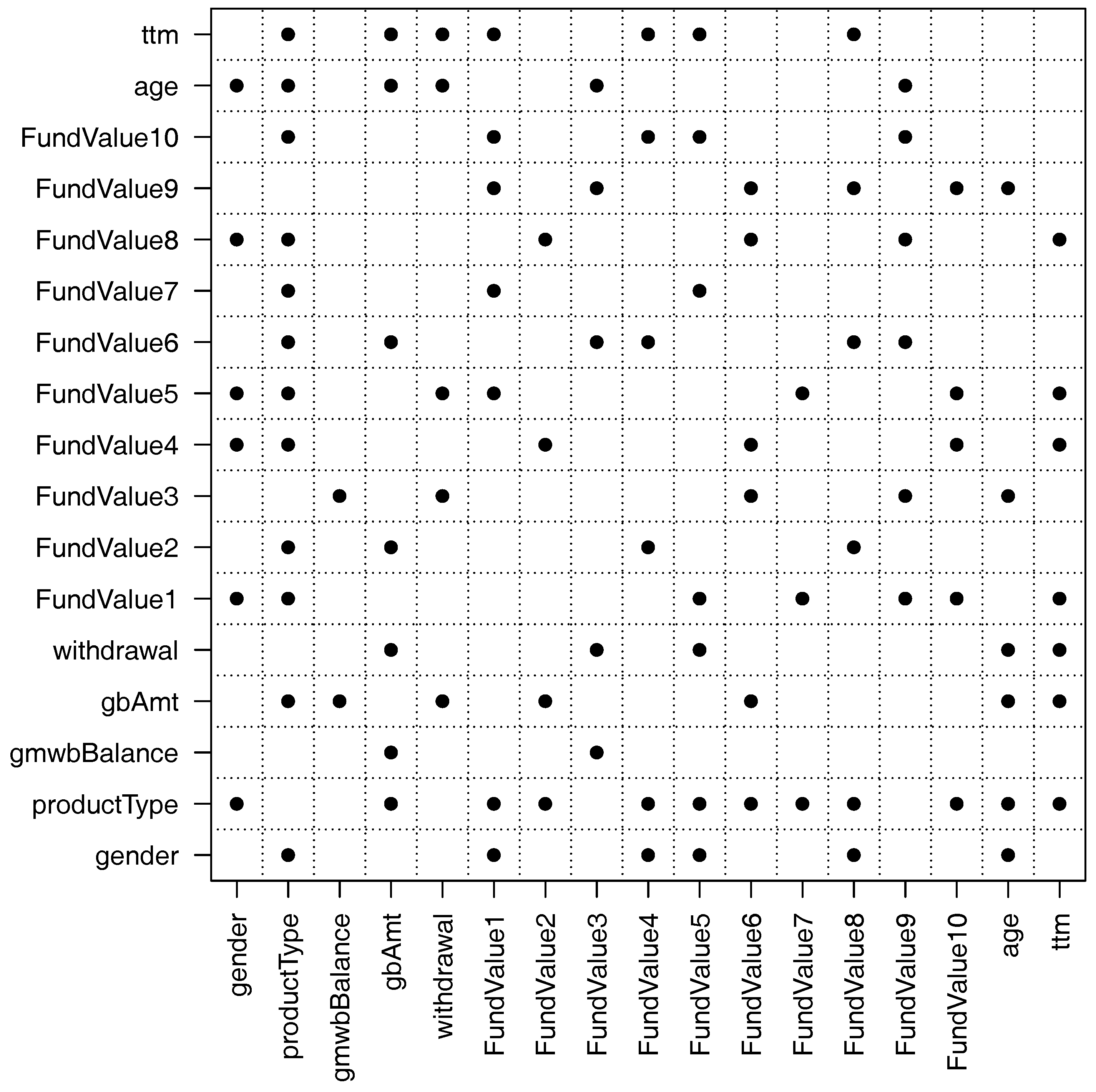
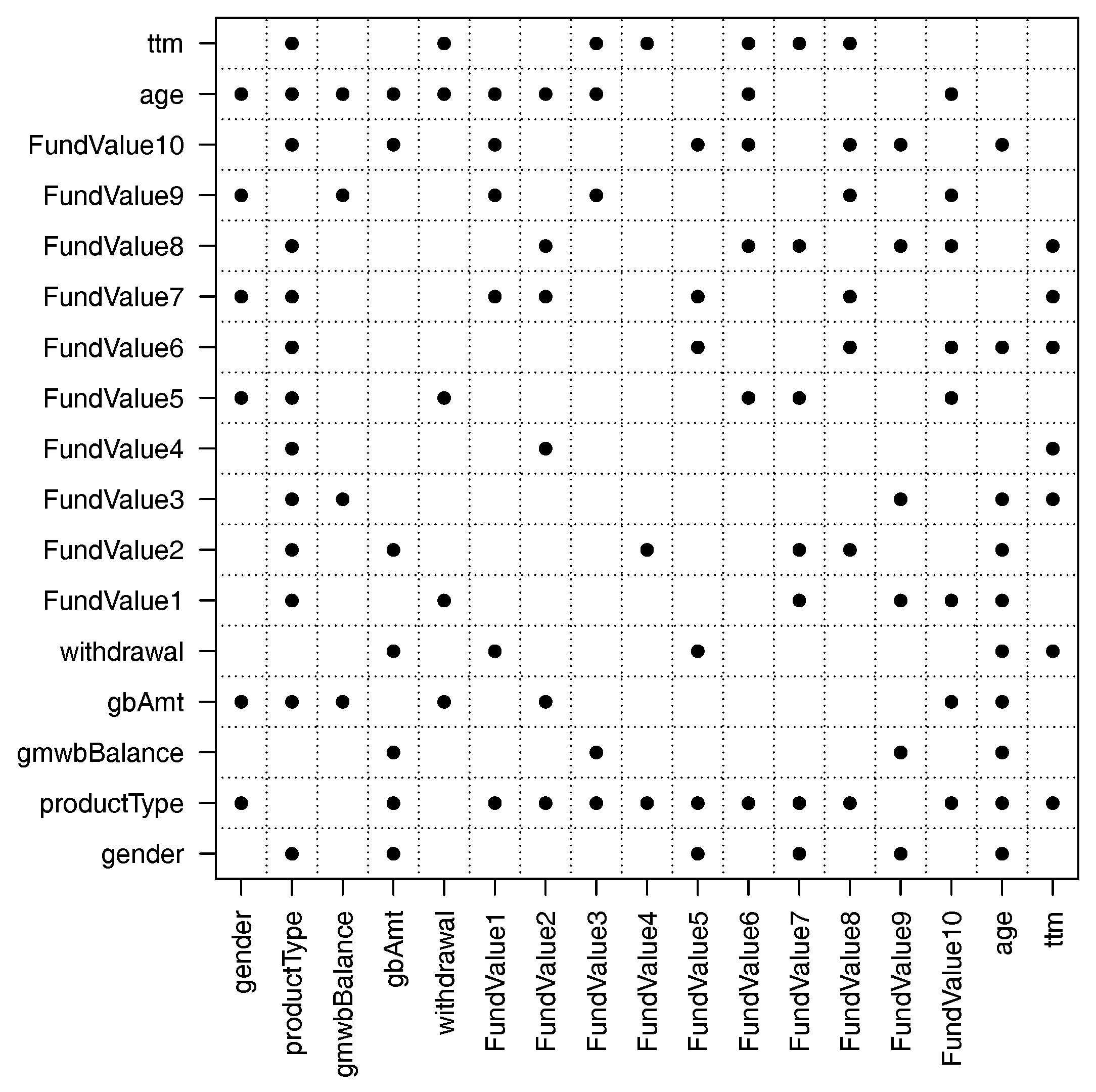
Figure 7 shows the important pairwise interactions found by the overlapped group-lasso. From the figure, we see that there are more than 50 pairwise interactions that are important. In particular, the variable productType has interactions with many other variables. This makes sense because the variable productType controls how the guarantee payoffs are calculated (see Gan and Valdez 2017b for details). The variable gmwbBalance has the fewest interactions with other variables. It has interactions with only two variables: gbAmt and FundValue3. The reason is that the variable gmwbBalance is zero for all contracts that do not include the GMWB guarantee.

Now let us look at how the models perform when we double the number of representative VA contracts.

Table 7. Accuracy and runtime of the metamodels when 680 representative VA contracts were used. The runtime is in seconds.

Model	PE	R2	CCC	Runtime
Linear Model without interactions	−0.0427	0.7963	0.8935	0.2000
Linear Model with interactions	0.0023	0.9589	0.9785	82.8800

shows the values of the validation measures and the runtime for the two models when 680 representative VA contracts were used. The values of the validation measures indicate that the linear model with interactions outperformed the linear model without interactions. The runtime shows that learning the important pairwise interactions takes some time. If we compare Table 7 to Table 5, we see that the performance of the linear model without interactions decreased when the number of representative contracts doubled. For example, the absolute value of the percentage error increased from 2.07% to 4.27% and the values of $R^2$ and $CCC$ also decreased slightly. This is counterintuitive because increasing the training samples usually leads to improvement in prediction accuracy. This might be related to the experimental design method we used. We used random sampling to select the representative VA contracts.

If we compare the values of the validation measures for the linear model with interactions in Table 5 and Table 7, we see that the accuracy of the linear model with interactions increased when we doubled the number of representative VA contracts. For example, the absolute value of the percentage error decreased from 0.36% to 0.23%, the $R^2$ increased from 0.9441 to 0.9589, and the $CCC$ increased from 0.9697 to 0.9785. The validation measures show that the impact of experimental design is not material when interactions are included. If we use a higher number of representative VA contracts, however, the runtime will increase due to the cross-validation.

Figure 8 shows the scatter plots between the fair market value calculated by Monte Carlo and those predicted by the linear models with and without interactions when 680 representative VA contracts were used. We see similar patterns as before when 340 representative VA contracts were used. Without interactions, the linear model did not fit the tails well.

Table 8. Summary statistics of the prediction errors of individual VA contracts when 680 representative VA contracts were used.

Model	Min	1st Q	Median	Mean	3rd Q	Max
Linear Model without interactions	−409.50	−27.48	3.40	2.89	30.54	737.49
Linear Model with interactions	−443.97	−10.26	−1.64	−0.61	6.72	456.92

shows some summary statistics of the prediction errors of individual VA contracts when 680 representative VA contracts were used. From the table, we again see that prediction errors of the linear model with interactions have a more symmetric distribution.

Figure 9 shows the QQ plots obtained by the linear models with and without interactions when 680 representative VA contracts were used. However, Figure 9b shows that even interactions were included, the fitting at the tails are a little bit off. The reason is that the distribution of the fair market values is highly skewed as shown in Figure 2.

Figure 10 shows the histograms produced by the linear models with and without interaction effects where 680 representative VA contracts were used. The histograms also show that the linear model with interactions outperforms the linear model without interactions.

Comparing Figure 8b, Figure 9b and Figure 10a to Figure 8a, Figure 9a and Figure 10a, we see that including interactions again increased the prediction accuracy.

Figure 11 and Figure 12 show respectively the cross-validation errors at different values of $\lambda$ and the important pairwise interactions found by the overlapped group-lasso when 680 representative VA contracts were used. We see similar patterns as before when 340 representative VA contracts were used. For example, the cross-validation error decreases when the value of $\lambda$ increases. The variable productType has interactions with many other variables. If we compare Figure 12 to Figure 7, however, we see that more interactions are found by the overlapped group-lasso when the number of representative VA contracts doubled.

In summary, our numerical results presented above show that including interactions in linear regression models is able to improve the prediction accuracy significantly.

6. Concluding Remarks

Using Monte Carlo simulation to value a large VA portfolio is computationally intensive. Recently, metamodeling approaches have been proposed to speed up the valuation of large VA portfolios and produce accurate results. The main idea of metamodeling is to build a predictive model based on a small number of representative VA contracts in order to reduce the number of contracts that are valued by Monte Carlo simulation. However, interaction effects between the contract features are not considered in existing metamodels.

In this paper, we investigated the effect of including interactions in linear regression models for the valuation of large VA portfolios. Since there are many features of a VA contract, there are a large number of possible interactions between the features. To select the important interactions, we used the overlapped group-lasso that can produce hierarchical interaction models. Our numerical results show that including interactions in linear regression models can lead to significant improvements in prediction accuracy. Since linear regression models are well known and well understood in statistics, the study of this paper shows that linear regression models with interaction effects are useful additions to the toolbox of metamodels that insurance companies can use to speed up the valuation of large VA portfolios.

References

1. Boyle, Phelim P., and Mary R. Hardy. 1997. Reserving for maturity guarantees: Two approaches. Insurance: Mathematics and Economics 21: 113–27. [Google Scholar] [CrossRef]
2. Brown, Robert A., Larry M. Gorski, and Thomas A. Campbell. 2002. Valuation and capital requirements for guaranteed benefits in variable annuities. Record 28: 1–22. [Google Scholar]
3. Cox, David R. 1984. Interaction. International Statistical Review/Revue Internationale de Statistique 52: 1–24. [Google Scholar] [CrossRef]
4. Dardis, Tony. 2016. Model efficiency in the U.S. life insurance industry. The Modeling Platform 3: 9–16. [Google Scholar]
5. Efron, Bradley, Trevor Hastie, Iain Johnstone, and Robert Tibshirani. 2004. Least angle regression. The Annals of Statistics 32: 407–51. [Google Scholar]
6. Frees, Edward W. 2009. Regression Modeling with Actuarial and Financial Applications. Cambridge: Cambridge University Press. [Google Scholar]
7. Gan, Guojun. 2013. Application of data clustering and machine learning in variable annuity valuation. Insurance: Mathematics and Economics 53: 795–801. [Google Scholar]
8. Gan, Guojun. 2015. Application of metamodeling to the valuation of large variable annuity portfolios. Paper presented at Winter Simulation Conference, Huntington Beach, CA, USA, December 6–9; pp. 103–14. [Google Scholar]
9. Gan, Guojun, and Jimmy Huang. 2017. A data mining framework for valuing large portfolios of variable annuities. Paper presented at the 23rd ACM SIGKDD International Conference on Knowledge Discovery and Data Mining, Halifax, NS, Canada, August 13–17; pp. 1467–75. [Google Scholar] [CrossRef]
10. Gan, Guojun, Qiujun Lan, and Chaoqun Ma. 2016. Scalable clustering by truncated fuzzy c-means. Big Data and Information Analytics 1: 247–59. [Google Scholar]
11. Gan, Guojun, and X. Sheldon Lin. 2015. Valuation of large variable annuity portfolios under nested simulation: A functional data approach. Insurance: Mathematics and Economics 62: 138–50. [Google Scholar] [CrossRef]
12. Gan, Guojun, and X. Sheldon Lin. 2017. Efficient greek calculation of variable annuity portfolios for dynamic hedging: A two-level metamodeling approach. North American Actuarial Journal 21: 161–77. [Google Scholar] [CrossRef]
13. Gan, Guojun, and Emiliano A. Valdez. 2016. An empirical comparison of some experimental designs for the valuation of large variable annuity portfolios. Dependence Modeling 4: 382–400. [Google Scholar] [CrossRef]
14. Gan, Guojun, and Emiliano A. Valdez. 2017a. Modeling partial greeks of variable annuities with dependence. Insurance: Mathematics and Econocmics 76: 118–34. [Google Scholar] [CrossRef]
15. Gan, Guojun, and Emiliano A. Valdez. 2017b. Valuation of large variable annuity portfolios: Monte carlo simulation and synthetic datasets. Dependence Modeling 5: 354–74. [Google Scholar] [CrossRef]
16. Gan, Guojun, and Emiliano A. Valdez. 2018. Regression modeling for the valuation of large variable annuity portfolios. North American Actuarial Journal 22: 40–54. [Google Scholar] [CrossRef]
17. Hardy, Mary. 2003. Investment Guarantees: Modeling and Risk Management for Equity-Linked Life Insurance. Hoboken: John Wiley & Sons, Inc. [Google Scholar]
18. Hejazi, Seyed Amir, and Kenneth R. Jackson. 2016. A neural network approach to efficient valuation of large portfolios of variable annuities. Insurance: Mathematics and Economics 70: 169–81. [Google Scholar] [CrossRef]
19. Hejazi, Seyed Amir, Kenneth R. Jackson, and Guojun Gan. 2017. A spatial interpolation framework for efficient valuation of large portfolios of variable annuities. Quantitative Finance and Economics 1: 125–44. [Google Scholar] [CrossRef]
20. Huang, Zhexue. 1998. Extensions to the k-means algorithm for clustering large data sets with categorical values. Data Mining and Knowledge Discovery 2: 283–304. [Google Scholar] [CrossRef]
21. Jaccard, James J., and Robert Turrisi. 2003. Interaction Effects in Multiple Regression, 2nd ed. Thousand Oaks: Sage Publications, Inc. [Google Scholar]
22. Ledlie, M. C., D. P. Corry, G. S. Finkelstein, A. J. Ritchie, K. Su, and D. C. E. Wilson. 2008. Variable annuities. British Actuarial Journal 14: 327–89. [Google Scholar] [CrossRef]
23. Lim, Michael, and Trevor Hastie. 2018. Learning Interactions via Hierarchical Group-Lasso Regularization. R Package Version 1.0.7. [Google Scholar]
24. Lim, Michael, and Trevor J. Hastie. 2015. Learning interactions via hierarchical group-lasso regularization. Journal of Computational and Graphical Statistics 24: 627–54. [Google Scholar] [CrossRef] [PubMed]
25. Lin, Lawrence I-Kuei. 1989. A concordance correlation coefficient to evaluate reproducibility. Biometrics 45: 255–68. [Google Scholar] [CrossRef] [PubMed]
26. Nawar, Sandra Maria. 2016. Machine Learning Techniques for Detecting Hierarchical Interactions in Insurance Claims Models. Master’s thesis, Concordia University, Montreal, QC, Canada. [Google Scholar]
27. The Geneva Association Report. 2013. Variable Annuities—An Analysis of Financial Stability. Available online: https://www.genevaassociation.org/sites/default/files/research-topics-document-type/pdf_public/ga2013-variable_annuities_0.pdf (accessed on 11 July 2018).
28. Tibshirani, Robert. 1996. Regression shrinkage and selection via the lasso. Journal of the Royal Statistical Society. Series B (Methodological) 58: 267–88. [Google Scholar]
29. Xu, Wei, Yuehuan Chen, Conrad Coleman, and Thomas F. Coleman. 2018. Moment matching machine learning methods for risk management of large variable annuity portfolios. Journal of Economic Dynamics and Control 87: 1–20. [Google Scholar] [CrossRef]
30. Yuan, Ming, and Yi Lin. 2006. Model selection and estimation in regression with grouped variables. Journal of the Royal Statistical Society, Series B (Methodological) 68: 49–67. [Google Scholar] [CrossRef] [Green Version]
Figure 1. Variable annuity sales in the US from 2008 to 2017. The numbers are obtained from LIMRA Secure Retirement Institute.
Risks 06 00071 g001
Figure 2. A histogram of the fair market values.
Risks 06 00071 g002
Figure 3. Scatter plots of the fair market values calculated by Monte Carlo simulation and those predicted by linear models when 340 representative VA contracts were used. The numbers are in thousands. (a) Without interactions; (b) With interactions.
Risks 06 00071 g003
0.490.49
(a)(b)
Figure 4. QQ plots of the fair market values calculated by Monte Carlo simulation and those predicted by linear models when 340 representative VA contracts were used. The numbers are in thousands. (a) Without interactions; (b) With interactions.
Risks 06 00071 g004
Figure 5. Histograms of the fair market values predicted by linear models when 340 representative VA contracts were used. The numbers are in thousands. (a) Without interactions; (b) With interactions.
Risks 06 00071 g005
Figure 6. Cross-validation errors at different values of the λ parameter when 340 representative VA contracts were used. The numbers are in thousands. (a) Cross-validation errors; (b) λ values.
Risks 06 00071 g006
Figure 7. Pairwise interactions found by the overlapped group-lasso when 340 representative VA contracts were used.
Risks 06 00071 g007
Figure 8. Scatter plots of the fair market values calculated by Monte Carlo simulation and those predicted by linear models when 680 representative VA contracts were used. The numbers are in thousands. (a) Without interactions; (b) With interactions.
Risks 06 00071 g008
Figure 9. QQ plots of the fair market values calculated by Monte Carlo simulation and those predicted by linear models when 680 representative VA contracts were used. The numbers are in thousands. (a) Without interactions; (b) With interactions.
Risks 06 00071 g009
Figure 10. Histograms of the fair market values predicted by linear models when 680 representative VA contracts were used. The numbers are in thousands. (a) Without interactions; (b) With interactions.
Risks 06 00071 g010
Figure 11. Cross-validation errors at different values of the λ parameter when 680 representative VA contracts were used. (a) Cross-validation errors; (b) λ values.
Risks 06 00071 g011
Figure 12. Pairwise interactions found by the overlapped group-lasso when 680 representative VA contracts were used.
Risks 06 00071 g012