A VaR-Type Risk Measure Derived from Cumulative Parisian Ruin for the Classical Risk Model

Département de mathématiques, Université du Québec à Montréal (UQAM), Montréal, QC H2X 3Y7, Canada
*
Author to whom correspondence should be addressed.
†
These authors contributed equally to this work.
Risks 2018, 6(3), 85; https://doi.org/10.3390/risks6030085
Submission received: 30 July 2018
/
Revised: 21 August 2018
/
Accepted: 23 August 2018
/
Published: 24 August 2018
(This article belongs to the Special Issue Risk, Ruin and Survival: Decision Making in Insurance and Finance)
Abstract
:In this short paper, we study a VaR-type risk measure introduced by Guérin and Renaud and which is based on cumulative Parisian ruin. We derive some properties of this risk measure and we compare it to the risk measures of Trufin et al. and Loisel and Trufin.
1. Introduction
Over the last few years, several dynamic risk measures, i.e., risk measures based on ruin-theoretic quantities, have been studied. For example, in the classical compound Poisson risk model, Trufin et al. (2011) considered a VaR-type risk measure defined as the smallest initial capital needed to ensure a certain probability of solvency throughout the lifetime of the surplus process. This risk measure has been extended by Mitric and Trufin (2016) who defined a risk measure taking into account both the probability of ruin and the expected deficit at ruin. In addition, Loisel and Trufin (2014) used the expected area below the solvency threshold as a risk indicator to introduce a new risk measure with some interesting properties.
Very recently, implementation delays in the recognition of ruin and occupation times of the surplus process have been used as alternative risk management tools to assess the quality of an insurance portfolio. In this direction, Guérin and Renaud (2017) introduced the concept of cumulative Parisian ruin, which is based on the time spent in the red by the underlying surplus process. The time of cumulative Parisian ruin is the first time the surplus process stays cumulatively below a critical level longer than a pre-determined grace period. Inspired by the risk measure of Trufin et al. (2011), they defined a VaR-type risk measure based on cumulative Parisian ruin. It is also defined as the smallest amount of capital for which the associated cumulative Parisian ruin probability is less than or equal to a tolerable level.
In this paper, we study this VaR-type risk measure based on cumulative Parisian ruin. In Guérin and Renaud (2017), this risk measure is proposed as a motivational reason to study the concept of cumulative Parisian ruin; the risk measure itself is neither analyzed nor used for any particular application. We derive some of its properties and compare it to the risk measures of Trufin et al. (2011) and Loisel and Trufin (2014).
The rest of the paper is organized as follows. In Section 2, we recall some background on the Cramér–Lundberg model, also known as the classical risk model, and define the concept of cumulative Parisian ruin. In Section 3, we introduce our risk measure and we give some of its properties. Finally, in Section 4, we study our risk measure in the special case of a Cramér–Lundberg process with exponential claims.
2. Insurance Risk Model
The Cramér–Lundberg model was proposed by Lundberg (1903) and further developed by Cramér (1930). In this model, the surplus process of an insurance company is modelled by
where and , and where is a compound Poisson process with a Poisson process of intensity and with positive random variables following a common cumulative distribution function . Recall that in this setup the claim sizes are mutually independent and are also independent of the number-of-claim process N. The process is known as the aggregate claim amount process. We call x the initial capital and c the premium rate.
We use the following equivalent notations to emphasize that the process X starts at level x. The notation corresponds to . When , we drop the index. In this model, the premium rate c is chosen usually to satisfy the net profit condition , which means that we can define the safety loading factor by .
The time of classical ruin associated to X is defined as
We denote the corresponding finite-time probability of ruin, for and , by
and the infinite-time probability of ruin by
Of course, we have .
In Trufin et al. (2011), assuming that the safety loading is fixed, the following ruin-consistent VaR-type risk measure is defined and analyzed: for a tolerance level , set
It is well known that we can compute using the Pollaczeck–Khinchine formula (also known in the actuarial literature as the Beekman’s convolution formula, see Beekman (1985)) which states that the probability of classical ruin is equal to the tail distribution function of a compound geometric random variable. First, let us define the aggregate loss at time t by and the maximal aggregate loss of the process by . The random variable L can be expressed as
where M is the number of record highs, which has a geometric distribution with success probability , and where are the ladder heights with common distribution . The Pollaczeck–Khinchine formula for the probability of ruin is then given by
where denotes the -th convolution of the distribution . Therefore, this risk measure can also be written as follows:
In some sense, the focus of this risk measure is shifted from the surplus process X to the distribution of the maximal aggregate loss L. This important relationship is at the core of the analysis done in Trufin et al. (2011). However, this relationship with the maximal aggregate loss L does not exist for the finite-time ruin probability. Note that this is also the case for the VaR-type risk measure defined and analyzed in Mitric and Trufin (2016).
Cumulative Parisian Ruin
Recently, Guérin and Renaud (2017) introduced a new definition of actuarial ruin based on the occupation-time process (below 0) associated with the surplus process X. The occupation-time process is defined as
Then, the time of cumulative Parisian ruin, with delay , is given by
In the definition of cumulative Parisian ruin, we aggregate the duration of all periods of financial distress until we accumulate r units of time spent in that red zone. Consequently, ruin is not declared as soon as X goes below zero: for , and , we have
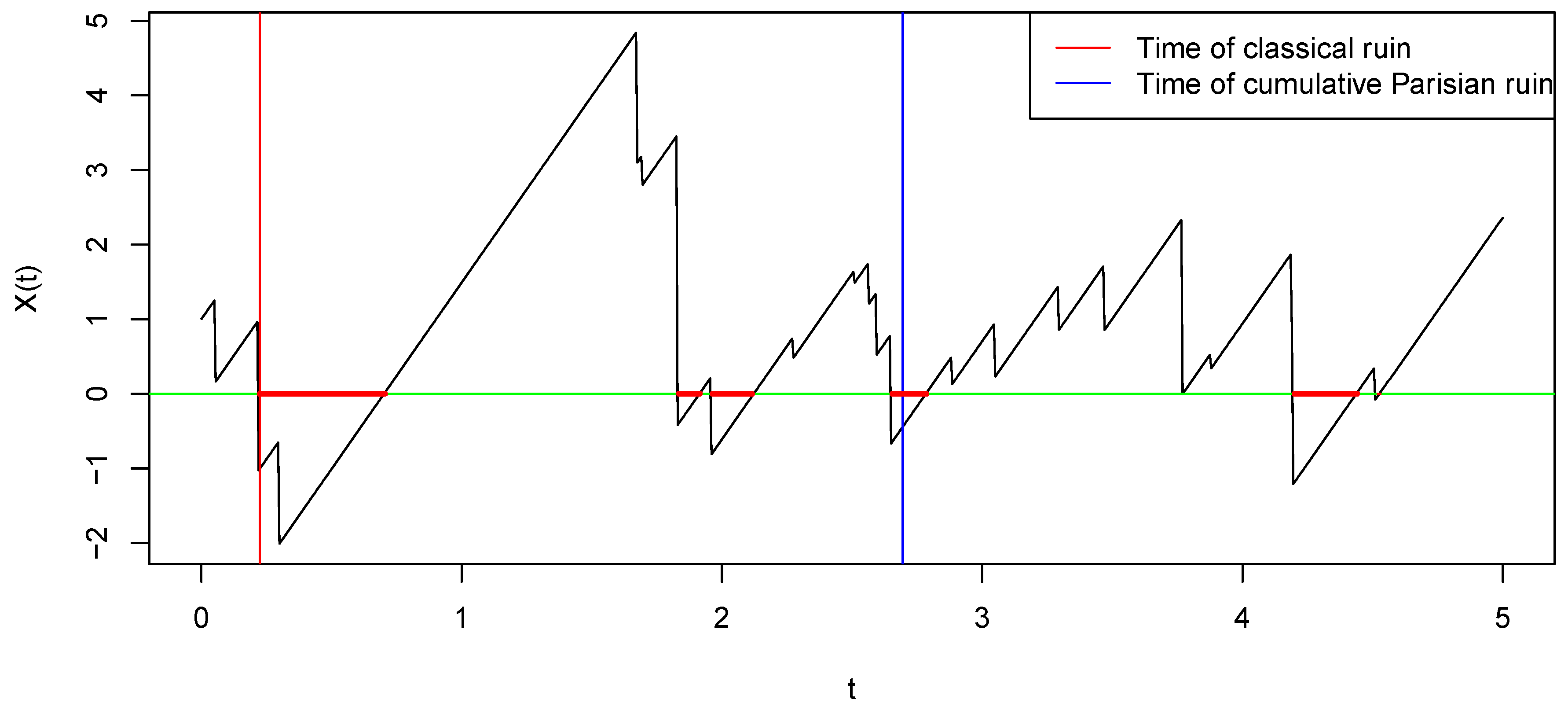
Cumulative Parisian ruin is somehow a generalization of classical ruin and, when , we recover the classical definition (see Guérin and Renaud (2017) for the details and see Figure 1 for a graphical comparison).
We denote the finite-time probability of cumulative Parisian ruin by
and the infinite-time version by
Of course, we have . With this new notation in hand, we can re-write the inequality in Equation (7) as follows: for , and , we have
We also have
3. A VaR-type Risk Measure Derived from Cumulative Parisian Ruin
Using the definition of cumulative Parisian ruin, Guérin and Renaud (2017) defined the following VaR-type risk measure: for a time horizon of length t and delay r, and for a given tolerance level , set
It gives the amount of initial capital needed in order to bound the finite-time probability of cumulative Parisian ruin with delay r by . Since , we can also write
Consequently, this risk measure is based on the distribution of . This is the analog of the random variable L for the risk measure in Equation (6). A major improvement is that we can now vary both the time horizon and the implementation delay by changing the values of t and r, respectively. The trade-off is that we need the distribution of a strongly path-dependent random variable, namely .
For the rest of this paper, we focus on the properties of this VaR-type cumulative Parisian risk measure. In addition, we compare the infinite-time version to the infinite-time risk measure defined in Trufin et al. (2011). Then, we also study the finite-time version as this is possible as soon as the distribution of is available.
Before going any further, let us give some background material on stochastic dominance.
3.1. Stochastic Dominance
Consider two random variables X and Y, and let and be their survival functions. We say that X is smaller than Y in the stochastic dominance order, which is denoted by , if
Equivalently, for all non-decreasing functions , we have
Here is a theorem taken from Shaked and Shanthikumar (2007).
Theorem 1.
- (i)
- Let and be two finite sets of independent random variables such that , for each . Then, for any increasing function , we have
- (ii)
- Consider two sequences of random variables and and two random variables X and Y such thatwhere denotes convergence in distribution. If for each n, then .
- (iii)
- Let the positive integer-valued random variable N be independent of the family of random variables and define . Define similarly .If and for each i, then
Finally, if and are stochastic processes, then we write if, for each , we have
The reader is referred to Shaked and Shanthikumar (2007), Kaas et al. (2008) and Denuit et al. (2005) for more details on stochastic ordering and applications in actuarial science.
3.2. Properties of the Risk Measure
In the following, let L and be two aggregate loss amount processes associated with two aggregate claim amount processes S and , themselves from two Cramér–Lundberg risk processes X and as defined in v(1).
Theorem 2.
For , and , we have:
- (i)
- Invariance by translation:For ,
- (ii)
- Positive homogeneity:For ,
- (iii)
- Monotonicity:If , then
Proof.
First, note that
Consequently,
This proves Equation (14).
Similarly, if we note that
then Equation (15) follows.
To prove the third property, we fix and we show that, if for all , then
First, let us define a sequence of discretized versions of the occupation-time process . For each , choose such that , as , and define
We define in the obvious way, i.e., when S is replaced by . We can re-write as follows:
where
Since for all , then we have for each i. Then, since
we have that for each i. From Equation (12), we obtain
or equivalently
Since and , by the second part of Theorem 1, we get
This means that
The property in Equation (16) follows. ☐
The monotonicity property in Equation (16) says that the risk measure is increasing with respect to the stochastic dominance order. Note that, if for all , then we can also prove that
If we put together the monotonicity property in Equations (16) and (13), then we can deduce the following intuitive relationship: a smaller frequency and a smaller severity yield less occupation time in the red zone and thus a smaller probability of cumulative Parisian ruin. For example, by the third part of Theorem 1, if C and are exponentially distributed random variables with parameters and , respectively, and if , and , then, for a given common premium rate c, the initial capital needed at a given tolerance level is larger for X than for .
It is worth mentioning that, as an immediate consequence of Proposition 1, Theorem 2 is also satisfied for the infinite-time horizon risk measure . Thus, we have recovered some of the results in Properties 3.1 and 3.2 of Trufin et al. (2011). In addition, an important consequence of Proposition 1 is the stochastic ordering for the finite-time ruin probability .
When there is no initial reserve, i.e., when , and for , the last theorem generalizes Theorem 4 in Goovaerts and De Vylder (1984) and also Proposition 1 of Lefèvre et al. (2017).
3.3. Relationship with Other Risk Measures
Recall that our main object of study is the following VaR-type risk measure: for , and ,
When , we write .
We are also interested in the risk measure based on the finite-time probability of classical ruin:
Using the inequality in Equation (9) and the discussions in the previous section, we deduce the following first proposition:
Proposition 1.
For a given time horizon and an acceptance level , the risk measure is less conservative than the risk measure , i.e.,
and, when , it converges to , i.e.,
When the implementation delay r is replaced by copies of an exponentially distributed random variable with rate , then, for , we have
In addition, in this case, cumulative Parisian ruin corresponds to Parisian ruin with exponential delays, that is
where is is the last time before t when the process was non-negative.
Hence,
We can then define the following VaR-type risk measure: for , and ,
In addition, we have
The risk measure satisfies the properties in Theorem 2. For example, we proved that, if , we have . Then, using Equation (12), we obtain
where Hence, using Equation (11), we get
and then
In addition, as an improvement of the finite-time version of the (infinite-horizon) risk measure defined by Loisel and Trufin (2014), we can define
where is a tolerance level for the expected area in the red defined as
where . Furthermore, we can use Theorem 1 of Loisel (2005) and then write
Remark 1.
Note that, with the distribution in Theorem 3, it is possible to compute the finite-time version of this risk measure based on the area in the red in the case of a Cramér–Lundberg process with exponential claims.
4. Example: Cramér–Lundberg Model with Exponential Claims
In this section, we want to see how reacts to changes in the value of its parameters. In other words, we want to perform a sensitivity analysis.
In general, we could use Monte Carlo simulations to compute values for . However, if we consider a Cramér–Lundberg process with exponentially distributed claims with rate parameter , then there exists an explicit expression for the distribution of the occupation time for a finite-time horizon. Unfortunately, such formulas are not available for most claim distributions.
Theorem 3
(Guérin and Renaud (2017)). For , we have
with
and
where represents the modified Bessel function of the first kind of order ν.
In Theorem 3, is the survival ruin probability over , that is
For an infinite-time horizon, we have the well-known expression:
From Corollary 2 in Renaud (2014), we can deduce the following expression for the distribution of , when the claims are exponentially distributed.
Corollary 1.
For any , we have
where is the incomplete gamma function.
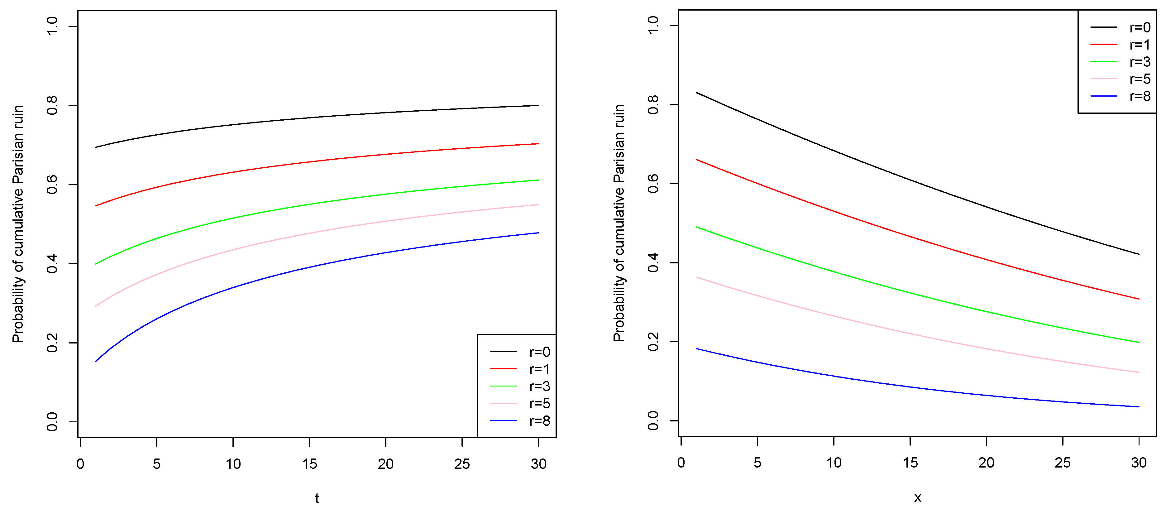
The explicit formula in Theorem 3 allows for a sensitivity analysis of the value of the probability of cumulative Parisian ruin, when claims are exponentially distributed, with respect to the delay parameter r and the time horizon t. In Figure 2, we observe that for a fixed delay parameter r, the probability of cumulative Parisian ruin increases when the time horizon t increases. This is because we accumulate more occupation time. On the other hand, it decreases when the delay r increases. For a fixed value of the time horizon t, increasing the initial capital x decreases the probability of cumulative Parisian ruin, as expected.
For the corresponding risk measures, Figure 3 illustrates the relationships in Equations (19) and in (20) between and . As , i.e., as the grace period gets smaller, the initial capital needed with increases toward that needed with , both at a tolerance level of . When the time horizon t increases, both risk measures increase the initial capital needed for that tolerance level.
5. Conclusions
In this paper, we study a VaR-type risk measure derived from cumulative Parisian ruin for the Cramér–Lundberg risk process. Precisely, this measure is defined as the smallest amount of capital for which the associated cumulative Parisian ruin probability is less than or equal to a tolerable level. We derive some properties of this risk measure and we provide some relationships with other risk measures. Finally, for exponentially distributed claims sizes, we performed sensitivity analysis of the values of the probability of cumulative Parisian ruin and the risk measure. Our risk measure could still be used for other risk processes such as the Brownian motion risk model.
Author Contributions
All the authors collaborated equally at every step of the research and in writing the paper.
Acknowledgments
Funding in support of this work was provided by the Natural Sciences and Engineering Research Council of Canada (NSERC). M.A.L. thanks the Institut des sciences mathématiques (ISM) and the Faculté des sciences at UQAM for their doctoral scholarships.
Conflicts of Interest
The authors declare no conflict of interest.
References
- Beekman, John A. 1985. A series for infinite time ruin probabilities. Insurance: Mathematics and Economics 4: 129–34. [Google Scholar] [CrossRef]
- Cramér, Harald. 1930. On the Mathematical Theory of Risk. Alingsås: Centraltryckeriet. [Google Scholar]
- Guérin, Hélène, and Jean-François Renaud. 2017. On the distribution of cumulative Parisian ruin. Insurance: Mathematics and Economics 73: 116–23. [Google Scholar] [CrossRef]
- Goovaerts, Marc, and F. Etienne De Vylder. 1984. Dangerous Distributions and Ruin Probabilities in the Classical Risk Model. Paper presented at the 22nd International Congress of Actuaries, Sydney, Australia, October 21–27; pp. 111–20. [Google Scholar]
- Denuit, Michel, Jan Dhaene, Marc Goovaerts, and Rob Kaas. 2005. Actuarial Theory for Dependent Risks: Measures, Orders and Models. New York: Wiley. [Google Scholar]
- Shaked, Moshe, and George Shanthikumar. 2007. Stochastic Orders. New York: Springer. [Google Scholar]
- Kaas, Rob, Marc Goovaerts, Jan Dhaene, and Michel Denuit. 2008. Modern Actuarial Risk Theory Using R. Berlin/Heidelberg: Springer. [Google Scholar]
- Loisel, Stéphane. 2005. Differentiation of some functionals of risk processes, and optimal reserve allocation. Journal of Applied Probability 42: 379–92. [Google Scholar] [CrossRef]
- Loisel, Stéphane, and Julien Trufin. 2014. Properties of a risk measure derived from the expected area in red. Insurance: Mathematics and Economics 55: 191–9. [Google Scholar] [CrossRef]
- Lefèvre, Claude, Julien Trufin, and Pierre Zuyderhoff. 2017. Some comparison results for finite-time ruin probabilities in the classical risk model. Insurance: Mathematics and Economics 77: 143–49. [Google Scholar] [CrossRef]
- Lundberg, Filip. 1903. I. Approximerad framställning af sannolikhetsfunktionen. II. Återförsäkring af kollektivrisker. Akademisk afhandling, etc. Uppsala: Almqvist & Wiksell. [Google Scholar]
- Renaud, Jean-François. 2014. On the time spent in the red by a refracted Lévy risk process. Journal of Applied Probability 51: 1171–88. [Google Scholar] [CrossRef]
- Mitric, Ilie-Radu, and Julien Trufin. 2016. On a risk measure inspired from the ruin probability and the expected deficit at ruin. Scandinavian Actuarial Journal 2016: 932–51. [Google Scholar] [CrossRef]
- Trufin, Julien, Hansjoerg Albrecher, and Michel Denuit. 2011. Properties of a risk measure derived from ruin theory. The Geneva Risk and Insurance Review 36: 174–88. [Google Scholar] [CrossRef]
Figure 1.
A sample path of a Cramér–Lundberg process . The time of ruin is in red and the time of cumulative Parisian ruin is in blue.
Figure 1.
A sample path of a Cramér–Lundberg process . The time of ruin is in red and the time of cumulative Parisian ruin is in blue.

Figure 2.
The probability of cumulative Parisian ruin for the Cramér–Lundberg process with , , , , and .
Figure 2.
The probability of cumulative Parisian ruin for the Cramér–Lundberg process with , , , , and .

Figure 3.
Risk measures and for the Cramér–Lundberg process with , , , , , and .

© 2018 by the authors. Licensee MDPI, Basel, Switzerland. This article is an open access article distributed under the terms and conditions of the Creative Commons Attribution (CC BY) license (http://creativecommons.org/licenses/by/4.0/).
Share and Cite
MDPI and ACS Style
Lkabous, M.A.; Renaud, J.-F. A VaR-Type Risk Measure Derived from Cumulative Parisian Ruin for the Classical Risk Model. Risks 2018, 6, 85. https://doi.org/10.3390/risks6030085
AMA Style
Lkabous MA, Renaud J-F. A VaR-Type Risk Measure Derived from Cumulative Parisian Ruin for the Classical Risk Model. Risks. 2018; 6(3):85. https://doi.org/10.3390/risks6030085
Chicago/Turabian StyleLkabous, Mohamed Amine, and Jean-François Renaud. 2018. "A VaR-Type Risk Measure Derived from Cumulative Parisian Ruin for the Classical Risk Model" Risks 6, no. 3: 85. https://doi.org/10.3390/risks6030085
Note that from the first issue of 2016, this journal uses article numbers instead of page numbers. See further details here.