
Evaluation of Pull Production Control Mechanisms by Simulation

Department of Industrial Engineering, Faculty of Mechanical Engineering and Naval Architecture, University of Zagreb, 10000 Zagreb, Croatia
*
Author to whom correspondence should be addressed.
Processes 2022, 10(1), 5; https://doi.org/10.3390/pr10010005
Submission received: 30 November 2021
/
Revised: 15 December 2021
/
Accepted: 17 December 2021
/
Published: 21 December 2021
(This article belongs to the Special Issue Process Control and Smart Manufacturing for Industry 4.0)
Abstract
:Today, companies need to continuously improve their production processes, which is a complex task. Lean manufacturing is one of the methodologies for production improvement, and one of the basic goals of any lean implementation is to reduce work-in-process (WIP) and shorten the production lead time. One of the basic lean principles for achieving these goals is pull principle. The adoption of this principle is quite challenging, as it requires a long-term commitment in the application and adoption of various lean techniques and tools that are prerequisites for the successful introduction of the pull principle. Kanban is the most well-known pull production control mechanism, and the first one developed within Toyota production system, but later, other pull control mechanisms were developed. Some of them include Conwip, Hybrid Kanban/Conwip, and Drum Buffer Rope (DBR), and those three, together with Kanban, were the research topic of this study. These four mechanisms were not explored and compared all together not for these specific production configurations considered in this research but also with regard to optimal parameters of control mechanisms. The goal was to analyze and compare how these pull control mechanisms affect lead time in different production conditions. For this purpose, simulation experiments were performed. The results showed that for different production conditions, different pull control mechanisms are optimal in terms of shortening lead time. This finding could help companies as a guideline for making a decision in terms of which pull control mechanism to choose.
1. Introduction
As demand for different types of products is advancing exponentially, more efficient production processes, innovative manufacturing models, and methods are becoming more important than ever. It goes without saying that manufacturing companies that want to survive must work continuously to improve their production. Many companies are introducing lean manufacturing to boost their competitiveness; thus, the study conducted by Industry Week and the Manufacturing Performance has found that the largest number (39%) of North American companies considered to be world-class manufacturers use lean manufacturing as the methodology for production improvement [1].
The concept of lean manufacturing originated from the Toyota production system (TPS). The main goal of the concept is to achieve production processes that respond quickly to changes in customer requirements, and this is possible if all waste is eliminated from production processes and with short production lead time [2,3]. John Krafcik coined the term “lean manufacturing” to describe TPS as lean production [4].
However, recently, the most researched topic in the field of manufacturing is Industry 4.0, lean manufacturing is still an important and significant topic both for manufacturing practices and scientific research. Thus, Buer and Strandhagen conducted extensive research concerning the relationship between Industry 4.0 and Lean manufacturing and made a conceptual framework that represents the relationships between Industry 4.0 and lean manufacturing, as well as their implications on performance and environmental factors. One of the relationships described states that Industry 4.0 can support and further develop lean manufacturing practices, which well demonstrates that the lean manufacturing concept is still very important in the context of manufacturing practices [5].
M.P. Ciano, P. Dallasega, and G.O.T. Rosii have also investigated the relationship between Industry 4.0 and lean manufacturing. They state that most studies find that lean manufacturing is a prerequisite for Industry 4.0, which can overcome barriers of lean manufacturing, but most studies miss an in-depth study of this topic on a practice technology level. As such, they conducted multiple case studies investigating these relationships. One of the relationships investigated is the importance of one-piece -flow, the concept from lean manufacturing, and its relationship to a successful implementation of the industry 4.0 [6]. One-piece-flow is one of the ideally achieved goals in any lean implementation. In his book, J. Womack defines lean as a set of five principles, with the two most important and most complex to achieve being the principles of flow and pull. Ideally, flow is a one-piece flow and the way to manage it is by pulling material in the production process. The first production control mechanism for achieving pull was Kanban.
The Kanban system was being developed by Toyota for over ten years; that is, it took Toyota over ten years in the 1950s to implement the idea of pulling material using signal cards. The reason for that was that there are several prerequisites for the successful implementation of such a system, and these are primarily small series or ideally one-piece flow, short set-up times, stable production process, i.e., production process with little variation and no downtime caused by any equipment failure, or some other disturbances [7,8].
In the last few decades, scientists and engineers from the field began to develop other systems similar to the Kanban signaling system for controlling material flow through the manufacturing process. Thus, to this day, several pull control mechanisms have been developed. The purpose of this study to was enable easier decision-making regarding pull control mechanism. The choice of pull strategy is dependent on the configuration of production processes. Pull control mechanisms have been researched extensively. The idea of this study was to evaluate four mechanisms that, according to researched literature, were not evaluated together specifically in production settings described in this study. In addition, most of the reviewed papers do not take into account optimal parameters of control mechanisms themselves which was also considered in this research.
Literature Review
Many studies have been conducted in order to define the optimal parameters of these control mechanisms [9,10,11,12,13], but also there are several studies answering the question of which control mechanism is a better choice in a given production setting. [14,15,16,17,18,19,20,21,22,23,24]. Some studies contradict each other [15,22], and despite the large number of comparisons of individual mechanisms, no research was done that would include a higher number of mechanisms and consider parameters that significantly affect the defined prerequisite for achieving pull. Therefore, it is necessary to conduct research that would consider the parameters that significantly affect the prerequisites for the successful application of production control mechanisms, and to determine which mechanism is a better choice for different values of these parameters.
Since the Kanban was developed in Toyota’s production facilities, the application of this pull control mechanism has become more present in different types of production processes. That was the reason behind the need for changing the characteristics of the pull control mechanism in order to adjust to individual needs of production processes. Thus, Monden has concluded that the traditional Kanban system has certain shortcomings, namely that it requires certain preconditions to be successfully applied, which are sometimes not so easy to achieve [7]. Some of these prerequisites are: variability in demand must be low (demand should be almost constant); product variety (production program) must be low; the process must be stable, without variations and machine set-up times should be kept to a minimum.
In 1990, Spearman, Woodruff and Hopp proposed another pull control mechanism, called “Constant Work in Process” (Conwip), which, unlike the classic Kanban system, limits the total amount of work-in-process, and signal cards exist only between the warehouse (where orders first arrive) and the first operation, and the further flow of material takes place according to FIFO (First in-First out) rule [25].
Boonlertvanich introduces another variant of the production management mechanism, which he concludes, has an advantage over both Kanban and Conwip. Boonlertvanich combines some features of Kanban, Conwip and Base Stocks and introduces a new mechanism called the “Extended Conwip-Kanban System” [26].
The fact that thirty-two different variants of the Kanban system have been developed and analyzed to date (of which nine variants have come to life in practice) shows how interesting the field of development of new variants of the Kanban signaling system has been to scientists and engineers [27]. Furthermore, to date, four different variants of the Conwip system have been developed [28].
The choice of the appropriate production management mechanism is very important. In some production conditions, the application of one machine will be more favorable in terms of achieving the shortest possible production lead time and as little work in process, which is the main goal of lean production, while in other conditions another mechanism will work better. It is up to the production manager to decide which mechanism to apply and define the optimal parameters of the selected mechanism. But how to make a good decision? What are the factors to consider when choosing a production control mechanism? If the process is not stable, i.e., the variability of individual parameters is quite high, will some other mechanism be more appropriate than a mechanism that would be appropriate in the same process but with small variations in parameters? According to Chao and Shih [29], there are forty-one parameters that affect the behavior of the production process. This piece of data alone indicates how complex the production process is and that defining the mechanisms which control the flow of materials through the production process is not such a simple task.
As the field of pull production control mechanisms has evolved, more and more scientists are comparing them to answer the question of which mechanism is more appropriate in the specific conditions of the production process. In general, all papers dealing with the comparison of production control mechanisms can be divided into two groups: research dealing with the study of production processes in which only one product is made [14,15,16,17,18,19,20,21,22,23,24], and research dealing with processes in which two or more products are produced [19,22,23,30].
The disadvantage of most comparisons is the lack of a unified framework for comparison. Namely, many studies do not consider the optimal parameters of the mechanisms they compare [15]. This is most likely why the conclusions are contradictory. For example, Lavoie, Gharbi and Kenne [15] conclude that in some situations Kanban is better, which is contrary to Bonvik’s conclusion [24]. Cheraghi et al. noted that Gastettner and Kuan analyzed Kanban and Conwip and concluded that choosing the best distribution of Kanban cards achieves less work in the process than with Conwip, which is contrary to Spearman’s work [22,25].
In order for the comparison to be correct, Amos et al. believes that each of the mechanisms should have optimal settings with respect to the given criteria and thus propose a methodology for comparing different mechanisms based on simulation experimentation and multicriteria optimization. In that work, Amos et al. compare Kanban, Conwip, and DBR in the production process of one product. They simulated an unbalanced production line consisting of 14 workstations and experimented by changing the location of a bottleneck in the process. The conclusion is that DBR is generally better than the Kanban and Conwip systems [14].
As an experimental factor in the comparison, many authors take the amount of stock in the buffers, which is defined by the size of the signal cards [15,17,21]. Lavoie, Gharbi and Kenne, monitor how the cost function behaves for different buffer sizes and conclude that the hybrid mechanism is better than Kanban and Conwip if the cost of storage is taken into account, but if these costs are not taken into account and only the cost of holding stocks is observed, then the hybrid mechanism and Conwip are equally good. Kanban becomes more financially viable if the cost of holding inventory and the number of operations increase [15].
Pettersen also takes the level of stocks in the buffers as an influential factor, but the frequency of machine downtime is taken as another parameter that influences the choice of mechanism. Pettersen compares Kanban and Conwip, simulating the production of a single product on a four-workstations production line and confirmed the advantage of Conwip over Kanban [16].
Enns and Rogers [21] also dealt with the problem of choosing a production control mechanism in the process of making a single product. They observed processing time and variability in demand by changing the rate of arrival of orders. In the end, they do not give an unambiguous conclusion as to which mechanism would be better under the stated conditions in production.
Bonvik, as well as Enns and Rogers, analyze the production of one product in conditions of different levels of demand, comparing Kanban, Conwip and Hybrid Kanban/Conwip mechanism, concluding that in most cases the Hybrid mechanism gives better results if the goal is to achieve less work in process and better service level [24].
Sharma and Agrawal [18] analyzed the behavior of the production system under different mechanisms (Kanban, Conwip, and Hybrid), also under conditions of variable demand. The production line of four workstations and the production of one product were analyzed. The results obtained by the AHP method were ranked and it was analyzed which alternatives are more suitable according to each criterion (minimum work in process, maximum production rate, etc.). Given the required criteria, the best choice of mechanism for different demand regimes (four different statistical distributions) was determined. The conclusion is that Kanban is better for three distributions, and Conwip for only one distribution [18].
Kabadurms [19] analyzed the production process of five different products by simulation experimentation and concluded that in conditions of variable demand the POLCA system (Paired Cell Overlapping by Card with Authorization) gives better results compared to Conwip, if the criterion is a small amount of work in the process and as short lead time. Kabadurms used the factorial design of the experiment by changing five parameters: coefficient of variation of processing time, orders arrival rate, batch size, number of process delays, and product variations.
Cheraghi [22] also analyzed a production line that produces more products, two different products specifically. He analyzed how batch size, demand frequency, and machine maintenance mode affect the total amount of work-in-process and the rate of production. He concluded that the frequency of demand significantly affects the behavior of production control mechanisms and concluded that pull production is not always the best choice compared to push when it comes to the criterion of reducing the total number of work-in-process.
In his doctoral dissertation, Terrence [23] also analyzes the production of several different products on the production line by comparing Kanban with the Economic Production Series (EPQ). The criteria for comparison were the work in process, the production cycle, the total production costs, and the influence of the machine set-up time. Terrence concludes that the time it takes to set up the machines significantly affects the production costs in both the Kanban and EPQ cases. However, in the case of a longer machine set-up time, EPQ is more cost-effective than Kanban. This is partly due to the larger production series of the EPQ, which reduces the frequency of machine adjustments. Costs are lower in the case of Kanban only when the set-up time is less than 15 min. Terrence concludes that the advantage of Kanban is that it gives flexibility to production, but does not take into account the variability of the level or frequency of demand which is a very important factor, but keeps demand constant and also does not take into account certain factors that can significantly influence behavior of production process, as well as on the choice of production control mechanism (variations in the duration of operations, process delays, etc.).
One of the factors that significantly affect the applicability and effectiveness of the production control mechanism is bottleneck. Among all researched literature, only Amos et al. [14] have investigated its influence on the performance of pull control mechanisms, Kanban, Conwip and DBR. But the influence of other factors, together with bottleneck, as well as their interaction, were not considered. In addition, the greater part of the researched literature considered two or three control mechanisms. The aim of this study was to evaluate only influence of the bottleneck together with another two factors, found in the literature, but also factors important for the successful implementation of pull principle from the authors’ experience. Those factors are variability in process and the time of operations. Together with those three factors, the influence of the selection of pull production control mechanism was evaluated. The idea was to analyze how the change in the characteristics of the production process, thus different levels of influence factors and the selection of production control mechanism affects the performance measurement of the production process, the lead time. The research goal was to determine under what conditions a certain production control mechanism is a better choice given the characteristics of the production process; thus the research questions are:
- Q1: Is there a performance difference between different pull production control mechanisms in terms of production lead time?
- Q2: Is the one pull production control mechanism that is optimal for one set of production conditions also optimal for another setting of production conditions?
2. Materials and Methods
In order to analyze the effects of factors (characteristics of the production process) on response (lead time), simulation experimentation and design of experiments were performed. The effect of the decision which production control mechanism to use in different production conditions (different levels of factors) on response criterion (lead time) was examined.
The pull mechanism is one of the basic principles of lean manufacturing [2]. The best way to describe it is to compare the pull mechanism with the push mechanism. Push mechanism is related to Material Resource Planning, and as Hopp and Spearman state, there is no other way of controlling work in the process other than work orders [8]. Figure 1 represents the production push system.
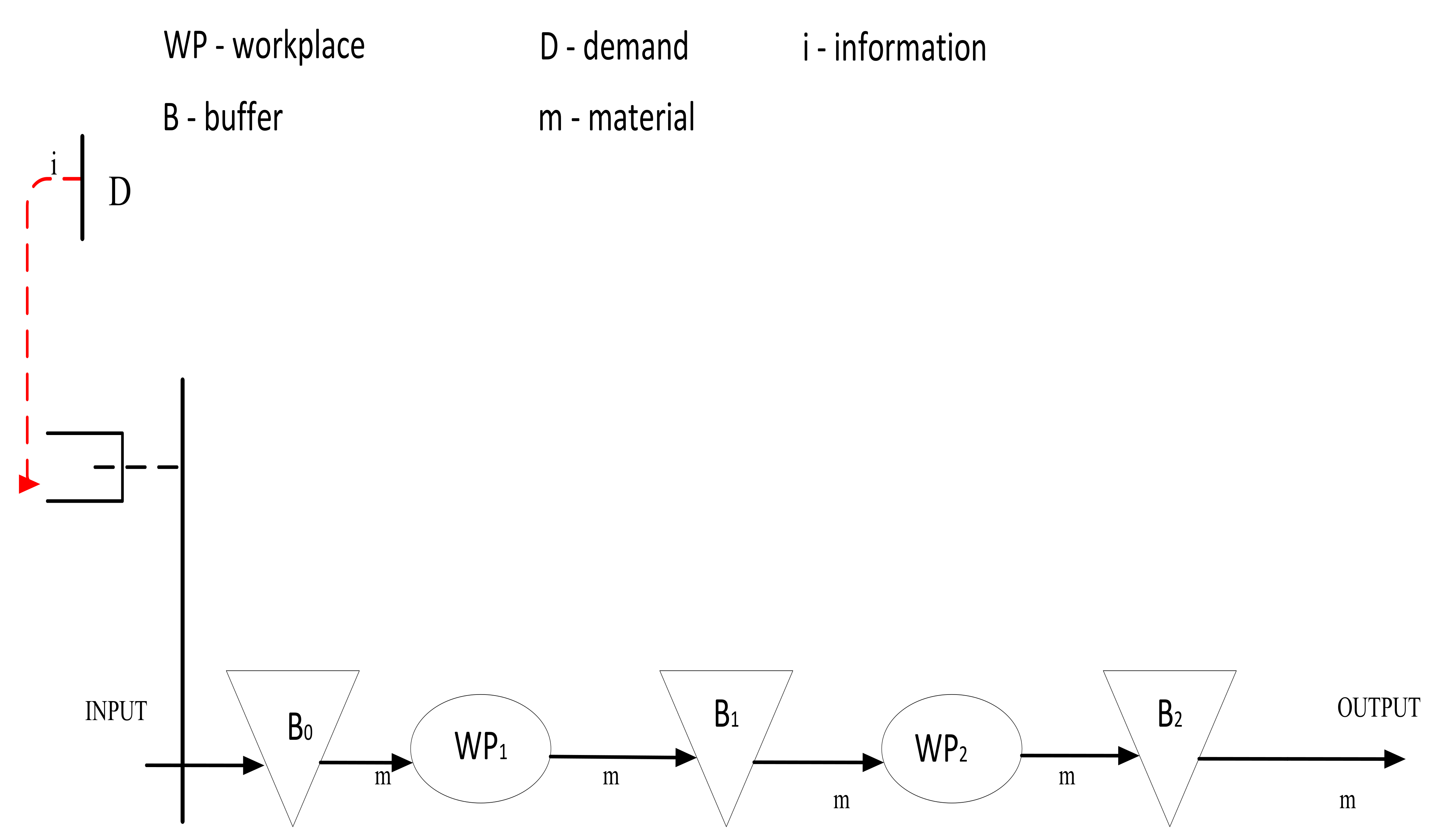
The flow of material in the push system is the same as in the pull system, but the rules defining how the information is distributed towards production stations are the key difference between the push and pull system [31]. Figure 2 represents the production pull system.
The fundamental difference between push and pull production systems, according to Hop and Spearman, is that the pull system explicitly restricts the work in process, while the push mechanism does not. They also state that there is a confusion and wrong perception that the difference between those two systems lies in the fact that push represents a make-to-stock system and pull represents a make-to-order system, which according to Hopp and Spearman is wrong. They state that this perception occurred after the releasing the book, Lean Thinking [2], where the authors define pull system as the rule that no one upstream in the production process can produce a product or service until the customer downstream requests one [8].
Hopp and Spearman also state that there is misunderstanding that pull mechanism is the synonym for Kanban system, while the true definition is that the Kanban system is only one of the mechanisms to achieve pull production. Although it indeed was the first production control mechanism developed in Toyota for achieving pull, later, other pull production control mechanisms were developed.
If one looks at the production system as a flow of information and a flow of materials, the flow of information is the one that triggers and control the flow of material. The information flow can be global and local. The global flow represents the information on customer demand, and the local flow is communication between different phases of the production process. [31]. The difference among all production control mechanisms is in the logic of distribution of both local and global information through the production process. Thus, every production control mechanism defines the flow of material by its own unique logic of the flow of information. [8].
Bicheno states that Kanban is one of the three most used production control mechanisms) for achieving a pull system. The other two most widely used mechanisms are CONWIP (“Constant work in process”) and DBR (Drum buffer rope) [32]. After reviewing the literature, it was decided to research these three mechanisms as well as Kanban/Conwip hybrid mechanism. Thus, the researched mechanisms are as follows:
- Kanban;
- Conwip;
- Kanban/Conwip hybrid;
- DBR.
3. Results
3.1. Simulation Model
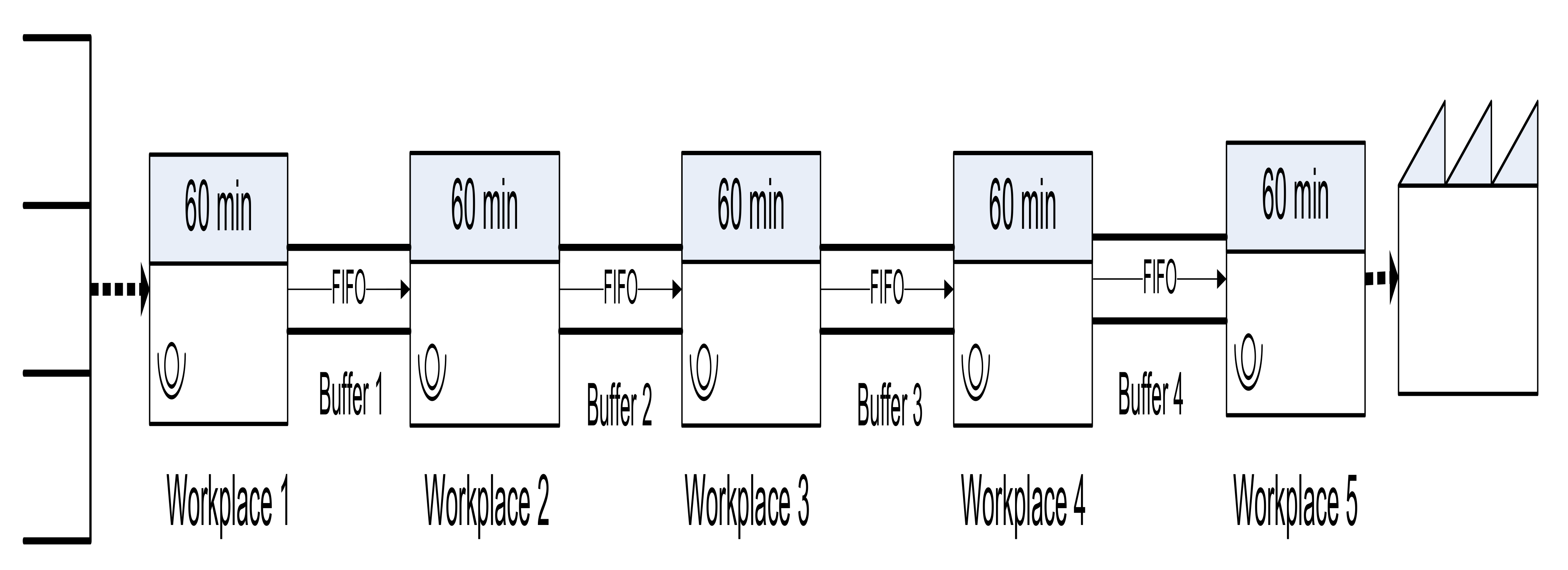
In order for the pull production control mechanisms to be compared and evaluated, simulation experimentation had to be performed. The first step was to build production process model. In the researched literature, it was found that the production line consisting of five workplaces present different enough aspects of production relationships and problems [23,33,34,35]. One such model was used in Enns and Rogers research paper [21]. The model consists of five workplaces, and every station presents a different operation, plus there is inventory between workplaces. This model was used for validation of the model in this research.
Figure 3 represents the model of the production process simulated in this study. The production begins at workplace number 1, then continues respectively through workplaces 2, 3, 4, and 5. The processing time is 60 min, while in the case of the existence of bottleneck, the processing time is 80 min. The production process begins at workplace 1 and continues at workplaces 2, 3, 4, and 5, respectively. The processing time on each machine is 60 min, and as one of the parameters is the existence, that is, the non-existence of a bottleneck. In the case of a bottleneck, the duration of the operation is 80 min. A lognormal distribution was used to generate processing time values. A review of the literature, but also conversations with experts dealing with this area, found that the lognormal distribution well the phenomena of processing time rather well. A new random number seed was used for each simulation run. This ensures the randomness of the generated values. For each level, i.e., a combination of input parameters, five simulation runs (five repetitions) was performed.
The assumptions for the model are consistent with the other studies [8,23,26,36], and are as follows:
- Each machine can only process one product in a time unit;
- Transport of the parts from the buffer to the next workplace follows the rule FIFO (first-in-first-out);
- Transport time between operations is negligible;
- One-piece flow production;
- Kanban system is the one-card Kanban system;
- Set-up time is not the subject of this research, so the production line produces one type of product;
- There is no storage of finished, good material and the material is always available from the raw material storage;
- Simulation time is 117,000 h (equals one year);
- Possible machine downtimes, waiting or any other stoppage of the process that may affect the processing time variability, are “covered” by the randomness of the processing time;
- Set-up time is not the subject of the research, so it is included in the processing time.
3.2. Validation of the Model
After the production process was modeled, it had to be validated. Two validation techniques were utilized. The first one is the comparison to other models technique and the other is the extreme condition test technique. Furthermore, all models were confirmed by Face validation in the way that three colleagues from the same field of research examined them and confirmed their validity [37]. Since the five-station model is also used in Enns and Rogers paper, their results could be compared with the ones that were gathered in this study. In their study, push and pull models were developed, and the pull model was controlled with the Conwip mechanism. Thus, as a first step, these two models were developed, and the results were compared. Simulation experimentation was performed in Simulink, a special module for the simulation in the MATLAB software, and since the discrete manufacturing production processes is simulated, an add-on for discrete simulation, SimEvents, was used [38]. After modeling and validation of these two models, all other mechanisms were modeled, Kanban, Hybrid Conwip/Kanban and DBR, respectively. The extreme condition test and face validation were performed.
In order to create the conditions for comparison, as in Enns and Roger’s article for comparison, the simulation time for the push and Conwip model was 101,000 min, and five runs were made for both push and Conwip. The processing time was chosen to be stochastic and is defined with operations time and coefficient of variation, cp, which is defined to be the standard deviation of the processing times divided by the mean processing time, 1/μ. The distribution used to generate processing times was the Gamma distribution, is defined by parameters α and β [21]. For the Conwip model, the number of control cards had to be the same; thus, six Conwip cards in the process were modeled. The results of comparison are given in Table 1.
Since the differences in results are insignificant, it could be concluded that the model for this research has a satisfactory range of accuracy, which is a match to the model presented and validated in the Roger and Enns research [21].
Further on, Kanban, Hybrid Conwip/Kanban and DBR were validated on the existing production model, validated previously by comparison. As already mentioned, the extreme condition test was used. In the case of Kanban, two extreme conditions were made:
- Extremely long operation time on the second workplace (85,000 min, which is 80% of the whole simulation run);
- The number of Kanban on the last workplace was set to be zero.
For the first condition, the result was that only one product came out of the process, which is expected since the second operation took 80% of time of the simulation run. And for the second condition, none of the products came out of the process, which also was expected. Since there were not any Kanban cards in the last workplace, thus there was no signal for processing. These results showed that the Kanban was well modeled.
The hybrid Kanban/Conwip control mechanism utilize both Conwip and Kanban cards in the process. Conwip cards regulate the overall amount of WIP, in a way that the information about demand is sent to the first stage of the production process, while the Kanban card sends the information about demand upstream starting from the last stage of the process up to the first one. Thus, Kanban cards regulate the amount of WIP at every production stage and unlike the Conwip cards that regulate the overall amount of WIP, thus the total amount of WIP in the whole process. The first extreme condition was as follows:
- The number of Conwip cards equals zero;
- The number of Kanban cards stays the same.
The second extreme condition was as follows:
- The number of Conwip cards stays the same;
- The number of Kanban cards changes in the fourth workplace and equals zero.
As expected, in both cases none of the products left the production process. In the first scenario, as the number of Conwip cards defines the total number of WIP in the production process, the WIP was zero, so the process could not produce any product. In the second scenario, just like in Kanban validation, as there were no control cards in the workplace, so there was no information for starting the production on that station. Again, none of the product left the process.
The same extreme condition, namely zero control cards, was used for DBR model and the same results were obtained.
3.3. Experiment Set-Up
In order to conduct the experiments, the level of the factors had to be chosen. But first, allow the decision of selected factors to be explained. There is an exact definition, found in literature, on what the prerequisites for successful implementation of pull production are:
- Balanced production process;
- Short set-up time;
- Constant customer demand;
- Production without downtimes [7].
Very often, these conditions are hard to achieve. Bottlenecks are quite a challenge in regard to production control. Thus, the question is whether, in these kinds of processes, a different control mechanism other than the Kanban is more suitable in terms of the efficiency of the production process. In addition, a smooth process, without stoppages is desirable, but the real processes are often faced with unexpected stoppages. From the authors’ experience, it is also known that the planned operation times are often different, due to many reasons, for example, a worker’s skills or frequent change of worker on the machines, requiring time for training, etc. All of this led to experimental factors chosen in this research:
- Variability of operation;
- Existence of a bottleneck in the process;
- Operation time;
- Number of control cards.
The last factor, the number of control cards, had been chosen because the production control mechanisms that were going to be examined in different production conditions (different level of experimental factors) have their own parameters that influence response function (lead time) that is being observed. Actually, the number of control cards, Kanban cards, Conwip cards, etc., is the parameter that had to be taken into account when considering efficient production flow. This parameter has not been considered much in previous research. Thus, many authors in the reviewed literature take the fixed number of cards, which they define as optimal and vary all other factors, but the optimal number of cards for one setting of factor levels does not have to suit different settings of factors level. This is the reason why the number of control cards has been taken as one of the experimental factors in this research.
The response function in this research is production lead time. The lead time is the total time elapsed from the moment when the material, i.e., the raw material, enters the production process to the moment when the finished product is ready for delivery to the customer [39]. Why has this response function been chosen? The goal of every lean implementation is to shorten the lead time [2], and since the topic of this research is one of the five basic principles of lean thinking [2], namely pull production, so this response function has been selected.
The levels of input parameters were defined after an extensive review of the literature and based on previous experience in various manufacturing companies. The levels are shown in Table 2.
As previously mentioned, the simulation model was developed in MATLAB, more precisely by Simulink and SimEvents, which are the features of MATLAB for simulation.
The Response Surface Methodology (RSM) was used to determine the effect of factors on response function; thus, the mathematical model was developed to describe the relationship between factor and response. The general factorial design was chosen to conduct the experiments. This experimental design was chosen because some of the varied factors (input variables) are numerical variables, and some are categorical variables. In such a case, it is convenient to use the general factorial design plan of the experiment. In the software package, Design Expert [40], which was used to analyze the results, this experimental plan is also called “multilevel categoric”.
After performing simulations followed by a designed experiment, an analysis of variance (ANOVA) was performed to determine the significance of the factors, and the mathematical model (response function) was developed by regression analysis. The factors of models A, B, C, and D are in order:
- A—coefficient of variation;
- B—operation time;
- C—the existence of a bottleneck;
- D—number of control cards.
3.4. Experiment Results
In the next part of the chapter, results of the experiments conducted Kanban-controlled processes will be described. This chapter will present the results of data analysis to describe the impact of processing time, coefficient of variation, bottleneck, and number of control cards on the lead time of the production process in the case of Kanban control mechanism. RSM was used to investigate the impacts of factors. Based on this method, a mathematical model was generated to describe the variable response.
Before analyzing the variance, it was necessary to make data transformation. In this data set, the ratio of the maximum and minimum measured value was greater than 10, so the transformation was required [40]. In this way, the homogeneity of variance over the experimental space is satisfied [41]. Data were transformed according to the equation:
y’ = ln (y + k), k = 0,
Variable y’ in the equation presents transformed value, and variable y presents the real value.
The bull hypothesis H0 for the experiment design was as follows: variability of processing time, processing time, bottleneck, and number of production control cards do not affect the lead time of the production process. Table 3 presents an analysis of variance (ANOVA) for the design of experiments. ANOVA generates significant factors of the model for the response while its significance was evaluated according to the probability levels. F-value shows that the model is significant. p-value also shows that the model is significant and that the null hypothesis can be rejected. Namely, the null hypothesis is rejected when the p-value is less than 0.05, which is the case here [40]. Furthermore, p-values of the factors A, B, C, and D, as well as their interactions AB, AD, BC, BD, CD, ABD, and BCD show their significance.
The next step was regression analysis, which is a method for estimating the relationships between a dependent variable and one or more independent variables. In this study dependent variable is lead time, while independent variables are: coefficient of variation, processing time, and existence of bottleneck. Based on the results obtained by simulation experimentation, the coefficients of the mathematical (regression) model were estimated.
The value of the coefficient of determination, R2, which is 0.9947 implied that the model is successful in explaining 99.47% of the experimental variables. In addition, the adjusted value of determination, the value of which is 0.9939 declared high significance of the generated model. These coefficients are in good relation. This is indicated by the necessary condition, which is that the difference between the adjusted R2 value and determination fitting R2 value is less than 0.2. When this condition is achieved it means that the obtained regression model (response function) is different from random phenomena (Table 4).
As the natural logarithm was used for data transformation, so the obtained mathematical model represents a mathematical function for calculating the lead time in logarithmic form. Thus, the calculated value should be transformed from a natural algorithm into a real number in order to obtain the actual value of the lea time variable.
ln (LTKanban) = 3.66826 − 0.002615Cv + 0.043041T + 0.194001Nr + 0.00809CvT + 0.008481CvNr
ln (LTKanban-BN) = 3.17249 + 0.244123Cv + 0.052751T − 0.327Nr − 0.001974CvT + 0.195583CvNr
Variables from Equations (2) and (3) are as follows:
- LTKanban—lead time for the process with without bottleneck, controlled by Kanban, min;
- LTKanban-BN—lead time for the process bottleneck controlled by Kanban, min;
- CV—coefficient of variation;
- T—processing time;
- Nr—number of control cards.
The value obtained by Equation (2) represents the natural logarithm of the lead time, and in order to get the actual value of the lead time, this value needs to be transformed into a real number using the equation:
LTKanban = eln(LTKanban)
The same mathematical relation as in Equation (4) has to be used for transforming natural logarithm values obtained by Equation (3) in order to get real number values.
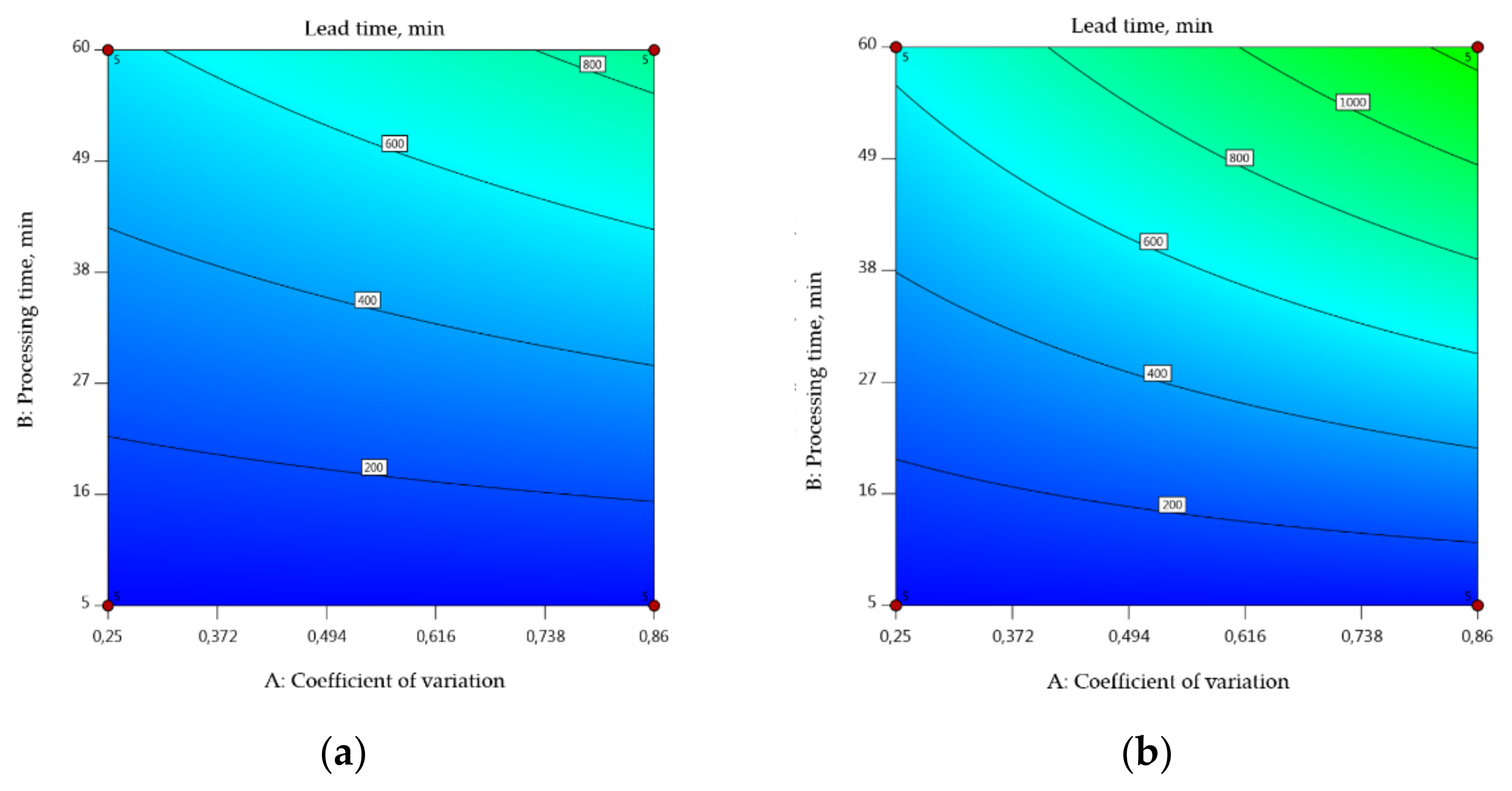
Figure 4a,b presents contour plots of mathematical model which describes the influence of factors and their interactions on the response function, in this case, lead time, for the production process controlled with Kanban. The first figure is for the process in which there are two Kanban cards in each phase of production, thus, for each operation and the second figure represents the process with five Kanban cards in each operation. Lead time, in the case of five Kanban cards, is much longer for the same level of the other factors in regards to the process with two Kanban cards. This was expected since the number of Kanban cards influences the level of work in the process, so the time needed for one piece of material to pass through the whole process is longer. Further experiments with other control mechanisms will show whether there is any difference between mechanisms for these same conditions.
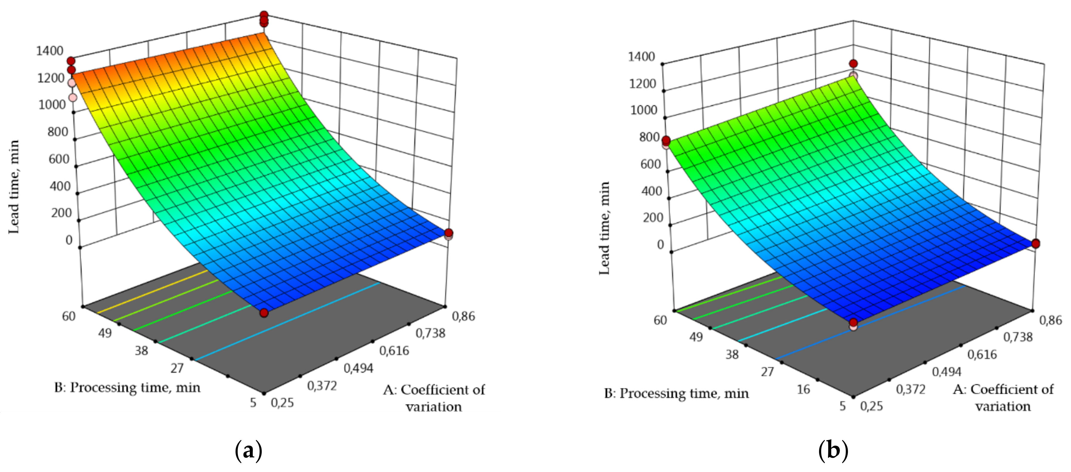
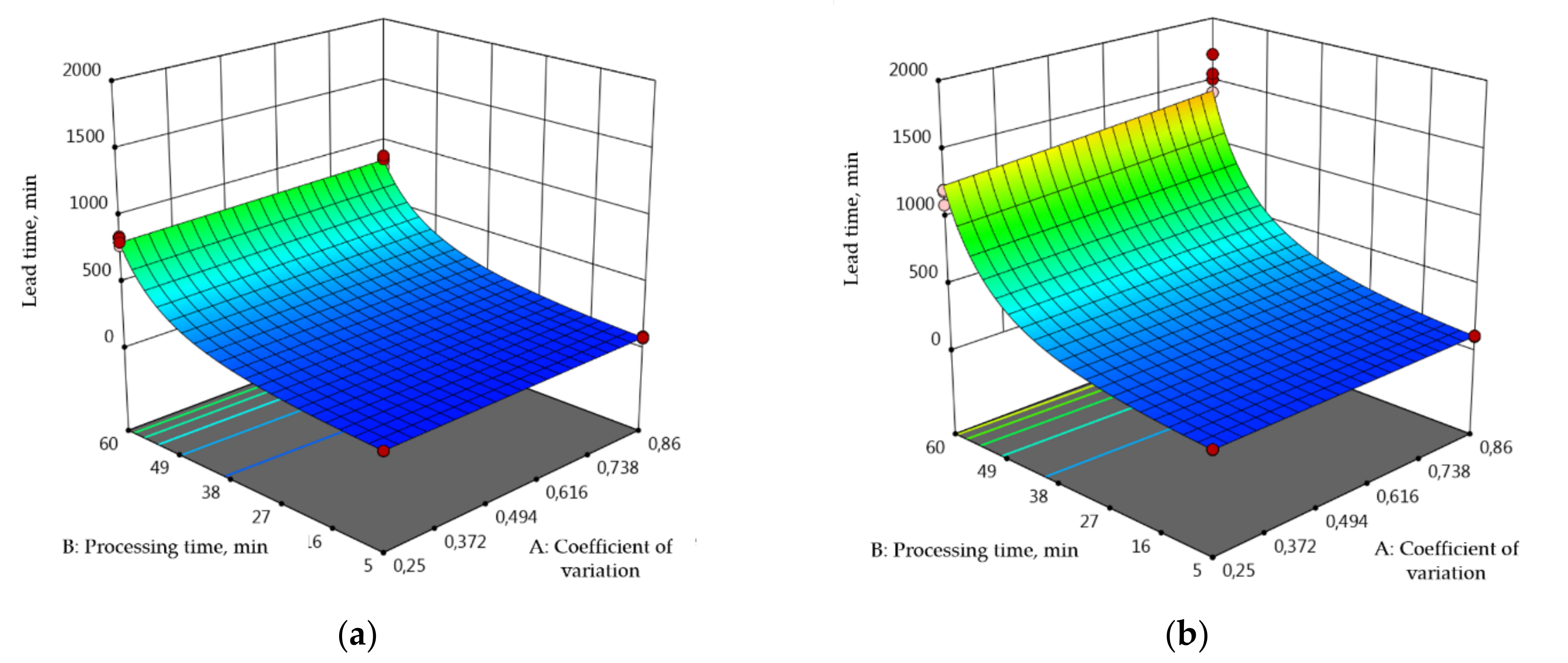
A three-dimensional 3D response surface plot showing the effect of coefficient of variation and operations is presented in Figure 5a,b—both figures present process with bottleneck with a difference in the number of Kanban cards. Number of Kanban cards affects the lead time quite significantly, as demonstrated below.
The same analysis, as presented for the case where Kanban mechanism was controlling simulated production process, was also conducted for Conwip, Hybrid Kanban/Conwip and DBR. The results are going to be presented further in this chapter.
For all three mechanisms, Conwip, Hybrid Kanban/Conwip and DBR, respectively, ANOVA has shown that both model and the factors are significant. Also, p-values of the factors A, B, C, and D, as well as their interactions AB, AD, BC, BD, CD, ABD, and BCD show their significance. As for the Kanban, based on the results obtained by simulation experimentation, the coefficients of the mathematical (regression) models were estimated. The coefficient of determination declared the significance of all models.
As for the analysis of variance for Kanban, in the case of Conwip, Hybrid Kanban/Conwip, and DBR, data transformation needed to be made for the same reason. In this way, the homogeneity of variance over the experimental space is satisfied [41]. In case of Conwip, the data were transformed according to the equation:
y’ = (y + k)λ, λ = 0.25
Variable y’ in the equation presents transformed value, and variable y presents the real value.
In case of Hybrid and DBR data were transformed according to the equation:
Table 8 represents the regression analysis for Conwip, Hybrid Kanban/Conwip and DBR. The values obtained for the regression functions are given in Table 9.
The value obtained by Equation (2) needs to be transformed into real values by using equation:
In the case of Hybrid and DBR, transformation should be made by the equation below.
y = 1/(y’)2
A three-dimensional 3D response surface plot showing the effect of coefficient of variation and processing time on lead time for the process with bottleneck is presented in Figure 6a,b. Both variations and processing time affects the lead time in terms that it gets longer, which was expected. Furthermore, the number of control cards has the same effect, which can be seen by comparing these two figures.
In the case of the hybrid mechanism, as presented in Figure 6, the lead time gets longer as the number of control cards is higher (Figure 7a,b). Every card tie one product, and more cards mean more products in the system, thus more work in process. But why would anybody make a decision to utilize more cards, one could ask. The answer is that the higher number of cards, meaning higher WIP, secures unstable processes and acts as a safety buffer, so the optimal solution has to be found.
As well as for Kanban, Conwip, Hybrid Kanban/Conwip, the same relationships between influence factors and response have been found for the DBR, as shown in Figure 8. Now, the question is which mechanism out of these four is optimal in regard to the same production conditions. That was also the research question of this study, and it will be explained further in the text based on the results shown thus far.
4. Discussion
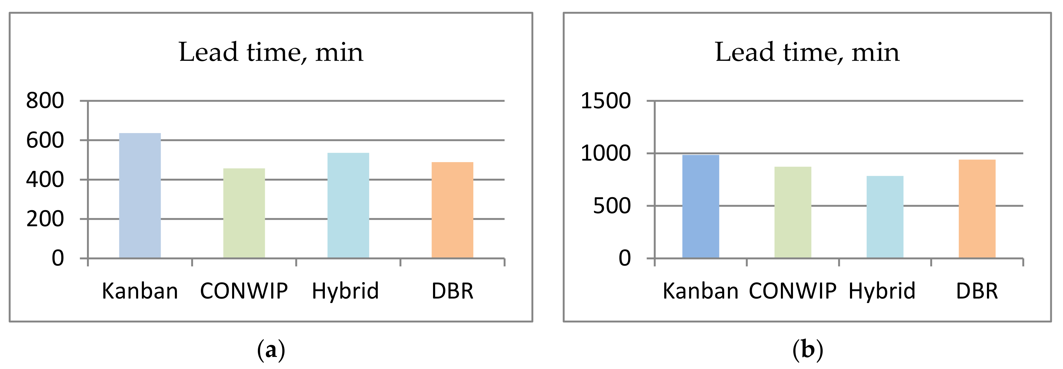
The pull principle is one of the five basic principles in lean manufacturing. It is the most important condition for achieving goals of lean manufacturing and that is flexible and customer-driven production, meaning ready to quickly respond to changes in demand. Prerequisites for pull are described in Monden’s work [7]. Some of these prerequisites, such as balanced production line and reduction of variability are explored in the work of Ertay T. [42]. However, in some cases, certain sources of variability in the process are not manageable at a given moment, but company can still have the positive effects of pull. In addition, balanced line due to existence of a bottleneck is not achievable at the given moment, but still, pull can bring positive effects in the process. As Hopp and Spearman state [8], it is quite common that Kanban is considered as a synonym for pull, but it is just one of the control mechanisms for achieving pull. In this study four different pull control mechanisms were explored, Kanban, Conwip, Hybrid Kanban/Conwip and DBR, respectively. The goal of this study was to evaluate these mechanisms in terms of their effectiveness, that is, how they affect lead time, which is one of the most important performance measures in terms of lean manufacturing. That effectiveness was evaluated by applying those control mechanisms in the same set of different production conditions. The conditions that were explored were existence of bottleneck in the production process, which has not been found a lot in the literature as a factor of research, and from the personal experience of the authors of this study, this factor was found to be one of the obstacles in achieving pull. The other two factors that were explored were variability and processing time as well as the number of signal cards, which is the parameter of control mechanism that ideally has to be optimal for a given condition. The response surfaces as well as regression functions that define relationships between lead time and described parameters, have been generated. Thus, lead time can be calculated for every combination of parameters. Response surfaces in Figure 5, Figure 6, Figure 7 and Figure 8 show these relations. For example, one possible combination of parameters describing the condition of production process could be as follows: coefficient of variation 0.2; processing time equals 40 min. Figure 9a,b shows the length of lead time for this combination of parameters in case when the overall number of signal cards is 15, where Figure 9a represents a case without bottleneck and Figure 9b with bottleneck. In practice, Kanban is very often the first considered mechanism for achieving pull, but as can be seen in Figure 9 and Figure 10, Kanban is not always the best solution.
Figure 9a and Figure 10a represent the relationship of the lead time and all four control mechanisms for the production process with lower and higher variability and with no bottleneck in the process.
Figure 9b and Figure 10b represent the relationship of the lead time and all four control mechanisms for the production process with lower and higher variability, but in this case, with the bottleneck in the process.
Figure 9 and Figure 10 show the length of lead time for all mechanisms for the same level of parameters except the variability. Figure 9a,b present production condition with low variability in the process (Cv = 0.2) and Figure 10a,b present production condition with a higher level of variability in the process (Cv = 0.86). If one compares the Figure 9a and Figure 10b, it can be concluded that for the same production conditions except one difference and that is variability, different pull control mechanisms contribute to the shorter lead time. Thus, in the process with lower variability the best choice is DBR, and in the process with higher variability the best choice is Conwip (Figure 9a and Figure 10a). The same comparison can be conducted for any combination of researched parameters.
Production managers and lean leaders often do not have time to test which control mechanism to implement in their production process. When lean implementation is in the phase of introducing and implementing pull, the question that arises is which control mechanism to apply. The results presented in this study could be applied in practice, as a guideline for selecting a production control mechanism depending on the condition of the production system. The decision process for the selection of production control mechanism could be as follows:
- Step 1: Define the current state of the production process in terms of variability, processing time and whether there is a bottleneck in the process;
- Step 2: Define the goal, that is minimal lead time;
- Step 3: Select the pull control mechanism using the findings obtained in this study.
Managing production and readiness to continuously improve production processes are challenging and never-ending tasks. As the literature suggests and practical experience supports, lean manufacturing is one of the methods that can help tremendously in achieving that task and is still widely used. Although every production process has its own characteristics, and solutions from one factory cannot be translated to another, some problems and obstacles are similar or the same. Organizing and managing a production process according to pull principles is a huge task for every factory; thus, any finding and guideline for making decisions about pull implementation could be useful. In that context, that was the goal of this research.
5. Conclusions
In this study, an evaluation of four pull production control mechanisms was conducted. The aim was to check if there is any performance difference between these mechanisms in terms of production lead time, and to investigate whether one mechanism which is optimal for certain set of production conditions is also optimal for another different setting. Specifically, for this study Kanban, Conwip, and DBR were chosen, because according to the literature, they are the most widely used pull control mechanisms, but also a hybrid mechanism, which is also commonly used. Parameters that define production conditions and that were in focus in this research were process variability, operation time and existence of bottleneck in the process. Some authors have investigated bottleneck as a parameter, for example, Amos et al., but they studied only Kanban, Conwip and DBR in that context, but not the Hybrid Kanban/Conwip mechanism. They found that DBR outperforms all others.
On the other hand, Bonvik et al. found that the Hybrid Kanban/Conwip outperforms Kanban and Conwip in the case of bottlenecks and high variability. The aim of this study was to include all of these four mentioned mechanisms, but also to consider the variability as a parameter which, for example, in Amos et al.’s study, was not taken into account, but the coefficient of variation was held constant. In addition, the scope of Bonvik et al. was service level and for Amos was a trade-off between throughput and WIP. In this study, regression functions for production lead time are gained, so for the different combinations of different levels of these factors, the optimal mechanism can be chosen.
The results showed that there is the performance difference between different pull production control mechanisms in terms of production lead time. One pull control mechanism that is the best choice for the setting of production conditions is not also the best choice for another set of production conditions. This is the answer to the research questions from the beginning of the study.
The limit of this study is that only the single-product process is explored. For future research, it would be interesting to explore multiple product lines, but also to explore other parameters, such as whether the length of the line together with all of parameters included in this study. Finally, for future research, it would be interesting to investigate these relationships in terms of different performance measures, which could be the goal of the companies in a given moment, such as productivity or service level.
Author Contributions
Conceptualization, N.T. and N.Š.; methodology, N.T.; software, N.T.; validation, N.T. and N.Š.; resources, N.T.; writing—original draft preparation, N.T.; writing—review and editing, N.T. and N.Š. All authors have read and agreed to the published version of the manuscript.
Funding
The Article Processing Charges (APCs) is funded by the European Regional Development Fund, grant number KK.01.1.1.07.0052.
Data Availability Statement
Data available on request.
Conflicts of Interest
The authors declare no conflict of interest.
References
- North America Manufacturing Benchmarks & Outlook for 2007, Analysis of Data from the IndustryWeek/Manufacturing Performance Institute Census of Manufacturers Conducted in the U.S. and the Canada Manufacturing Study. Available online: http://www-03.ibm.com/marketing/edocument/industrial/lgh_eas_manufacturing_kit/document/print/print.pdf (accessed on 19 April 2021).
- Womack, J.P.; Jones, D.T. Lean Thinking: Banish Waste and Create Wealth in Your Corporation, 2nd ed.; Simon and Schuster: New York, NY, USA, 2003. [Google Scholar]
- Murman, E.; Allen, T.; Bozdogan, K.; Cutcher-Gershenfeld, J.; McManus, H.; Nightingale, D.; Rebentisch, E.; Shields, T.; Stahl, F.; Walton, M.; et al. Lean Enterprise Value: Insights from MIT’s Lean Aerospace Initiative; Palgrave: New York, NY, USA, 2002. [Google Scholar]
- Womack, J.P.; Jones, D.; Roos, D. The Machine That Changed the World; Simon and Schuster: London, UK, 1990. [Google Scholar]
- Buer, S.-V.; Strandhagen, J.O.; Chan, F.T.S. The link between Industry 4.0 and lean manufacturing: Mapping current research and establishing a research agenda. Int. J. Prod. Res. 2018, 56, 2924–2940. [Google Scholar] [CrossRef] [Green Version]
- Ciano, M.P.; Dallasega, P.; Orzes, G.; Rossi, T. One-to-one relationships between Industry 4.0 technologies and Lean Production techniques: A multiple case study. Int. J. Prod. Res. 2021, 59, 2021. [Google Scholar] [CrossRef]
- Monden, Y. Toyota Production System: An Integrated Approach to Just-In-Time, 4th ed.; Taylor & Francis Group: Abingdon, UK, 2012. [Google Scholar]
- Hopp, W.J.; Spearman, M.C. Factory Physics, 3rd ed.; Waveland Press Inc.: Long Grove, IL, USA, 2008. [Google Scholar]
- Chan, F.T.S. Effect of Kanban size on just in time manufacturing systems. J. Mater. Process. Technol. 2001, 116, 146–160. [Google Scholar] [CrossRef]
- Jodlbauer, H. Customer driven production planning. Int. J. Prod. Econ. 2008, 111, 793–801. [Google Scholar] [CrossRef]
- Baykoc, O.F.; Erol, S. Simulation modeling and analysis of JIT production system. Int. J. Prod. Econ. 1998, 55, 203–212. [Google Scholar] [CrossRef]
- Enns, S.T. Pull replenishment performance as a function of demand rates and setup times under optimal settings. In Proceedings of the 2007 Winter Simulation Conference, Washington, DC, USA, 9–12 December 2007; pp. 1624–1632. [Google Scholar]
- Yang, L.; Zhang, X.P. Design and Application of Kanban Control System in a Multi-Stage, Mixed-Model Assembly Line. Syst. Eng. Theory Pract. 2009, 29, 64–72. [Google Scholar] [CrossRef]
- Amos, H.C.N.; Bernedixen, J.; Syberfeldt, A. A comparative study of production control mechanisms using simulation-based multi-objective optimization. Int. J. Prod. Res. 2012, 50, 359–377. [Google Scholar]
- Lavoie, P.; Gharbi, A.; Kenne, J.P. A comparative study of pull control mechanisms for unreliable homogenous transfer lines. Int. J. Prod. Econ. 2010, 124, 241–251. [Google Scholar] [CrossRef]
- Pettersen, J.A. Pull Based Production Systems—Performance, Modeling and Analysis. Ph.D. Thesis, Lulea University of Technology, Lulea, Sweden, 2010. [Google Scholar]
- Pettersen, J.A.; Segerstedt, A. Restricted work-in-process: A study of differences between Kanban and CONWIP. Int. J. Prod. Econ. 2009, 118, 199–207. [Google Scholar] [CrossRef]
- Sharma, S.; Agrawal, N. Selection of a pull production control policy under different demand situations for a manufacturing system by AHP-algorithm. Comput. Oper. Res. 2009, 36, 1622–1632. [Google Scholar] [CrossRef]
- Kabadurmus, O. A comparative study of POLCA and Generic CONWIP production control systems in erratic demand conditions. In Proceedings of the IIE Annual Conference, Miami, FL, USA, 30 May–3 June 2009. [Google Scholar]
- Sandanayake, Y.G.; Oduoza, C.F.; Proverbs, D.G. A systematic modeling and simulation approach for JIT performance optimization. Robot. Comput. Integr. Manuf. 2008, 24, 735–743. [Google Scholar] [CrossRef]
- Enns, S.T.; Rogers, P. Clarifying CONWIP versus PUSH system behavior using simulation. In Proceedings of the 2008 Winter Simulation Conference, Miami, FL, USA, 7–10 December 2008; pp. 1867–1872. [Google Scholar]
- Cheraghi, H.S.; Dadashzadeh, M.; Soppin, M. Comparative Analysis of Production Control Systems Through Simulation. J. Bus. Econ. Res. 2008, 66, 88–104. [Google Scholar] [CrossRef] [Green Version]
- Terrence, M.J. A Simulation and Evaluation Study of the Economic Production Quantity Lot Size and Kanban for Single Line, Multi—Product Production System Under Various Setup Times. Ph.D. Thesis, Kent State University, Kent, OH, USA, 2008. [Google Scholar]
- Bonvik, A.M.; Couch, C.; Gershwin, S.B. A Comparison of Production-line Control Mechanisms. Int. J. Prod. Res. 1997, 35, 789–804. [Google Scholar] [CrossRef]
- Spearman, M.L.; Woodruff, D.L.; Hopp, W.J. CONWIP: A Pull Alternative to Kanban. Int. J. Prod. Res. 1990, 28, 879–894. [Google Scholar] [CrossRef]
- Boonlertvanich, K. Extended CONWIP-Kanban System: Control and performance. Ph.D. Thesis, Georgia Institute of Technology, Atlanta, GA, USA, 2005. [Google Scholar]
- Lage, J.M.; Filho, M.G. Variations of the Kanban system: Literature review and classification. Int. J. Prod. Econ. 2010, 125, 13–21. [Google Scholar] [CrossRef]
- Prakash, J.; Chin, J.F. Variation of CONWIP Systems. World Acad. Sci. Eng. Technol. 2012, 6, 2765–2769. [Google Scholar]
- Chao, H.; Shih, W.L. Simulation studies in JIT production. Int. J. Prod. Res. 1992, 30, 2573–2586. [Google Scholar] [CrossRef]
- Torkabadi, A.; Mayorga, R. Evaluation of pull production control strategies under uncertainty: An integrated fuzzy AHP-TOPSIS approach. J. Ind. Eng. Manag. 2018, 11, 161–184. [Google Scholar] [CrossRef]
- Askin, R.G.; Goldberg, J.B. Design and Analysis of Lean Production Systems; John Wiley & Sons: New York, NY, USA, 2002. [Google Scholar]
- Bicheno, L. The New Lean Toolbox: Towards Fast Flexible Flow; Picsie Books: Buckingham, UK, 2004. [Google Scholar]
- Darlingtona, J.; Francisb, M.; Foundc, P.; Thomasc, A. Design and implementation of a Drum-Buffer-Rope pull-system. Prod. Plan. Control. 2015, 26, 489–504. [Google Scholar] [CrossRef]
- Marek, R.P.; Elkins, D.A.; Smith, D.R. Understanding the fundamentals of Kanban and CONWIP pull systems using simulation. In Proceedings of the Winter Simulation Conference, Arlington, VA, USA, 9–12 December 2001. [Google Scholar]
- Rotaru, A. Performance Analyses of Conwip—Base stock controlled production system using simulation. In Scientific Bulletin, Automotive Series; Faculty of Mechanics and Technology, University of Pitesti: Pitești, Romania, 2011; Volume XVI. [Google Scholar]
- Sergent, R.G. Verification and validation of simulation models. In Proceedings of the 2010 Winter Simulation Conference, Baltimore, MD, USA, 5–8 December 2010. [Google Scholar]
- Matlab, R. Model and Simulate Message Communication and Discrete-Event Systems. 2017. Available online: https://www.mathworks.com/products/simevents/whatsnew.html (accessed on 17 November 2017).
- Gestettner, S.; Kuhn, H. Analysis of production control systems Kanban and Conwip. Int. J. Prod. Res. 1996, 34, 3253–3273. [Google Scholar] [CrossRef]
- Design-Expert® Software, Version 11. Available online: https://www.statease.com/dx11.html (accessed on 14 November 2017).
- Pavlić, I. Statistička teorija i primjena, Tehnička knjiga Zagreb. Color Plates 2004, 48, 239. [Google Scholar]
- Cajner, H.; Tonković, Z.; Šakić, N. The significance of data transformation in analysis of experiments. In Proceedings of the 12th International Scientific Conference on Production Engineering (CIM 2009), Biograd, Croatia, 17–20 June 2009. [Google Scholar]
- Ertay, T. Simulation approach in comparison of a pull system in a cell production system with a push system in a conventional production system according to flexible cost: A case study. Int. J. Prod. Econ. 1988, 56–57, 145–155. [Google Scholar] [CrossRef]
Figure 1.
Production push system.

Figure 2.
Production pull system.

Figure 3.
Production process.

Figure 4.
Response surface contour plots: (a) Effects of coefficient of variation and operation time on lead time for the process without bottleneck and two Kanban cards in each operation; (b) Effects of coefficient of variation and operation time on lead time for the process without a bottleneck and five Kanban cards in each operation.

Figure 5.
Response surface 3D plots: (a) Effects of coefficient of variation and operation time on lead time for the process with bottleneck and two Kanban cards in each operation; (b) Effects of coefficient of variation and operation time on lead time for the process with bottleneck and five Kanban cards in each operation.

Figure 6.
Response surface 3D plots: (a) Effects of coefficient of variation and operation time on lead time for the process with bottleneck and three Conwip cards in each operation (15 cards for the whole process); (b) Effects of coefficient of variation and operation time on lead time for the process with bottleneck and two Conwip cards in each operation (10 cards for the whole process.

Figure 7.
Response surface 3D plots: (a) Effects of coefficient of variation and operation time on lead time for the process with bottleneck and two cards in each operation; (b) Effects of coefficient of variation and operation time on lead time for the process with bottleneck and three cards in each operation.

Figure 8.
Response surface 3D plots: (a) Effects of coefficient of variation and operation time on lead time for the process with bottleneck and nine DBR cards in the whole process; (b) Effects of coefficient of variation and operation time on lead time for the process with bottleneck and 14 DBR cards in the whole process.

Figure 9.
Comparison of the lead time for each control mechanism under the same production condition: (a) CV = 0.2 and T = 40 min for the process without bottleneck and WIP = 15; (b) CV = 0.2 and T = 40 min, for the process with bottleneck and WIP = 15.
Figure 9.
Comparison of the lead time for each control mechanism under the same production condition: (a) CV = 0.2 and T = 40 min for the process without bottleneck and WIP = 15; (b) CV = 0.2 and T = 40 min, for the process with bottleneck and WIP = 15.

Figure 10.
Comparison of the lead time for each control mechanism under the same production condition: (a) CV = 0.86, and T = 40 min, for the process without bottleneck and WIP = 15; (b) CV = 0.86 and T = 40 min, for the process with bottleneck and WIP = 15.
Figure 10.
Comparison of the lead time for each control mechanism under the same production condition: (a) CV = 0.86, and T = 40 min, for the process without bottleneck and WIP = 15; (b) CV = 0.86 and T = 40 min, for the process with bottleneck and WIP = 15.


Table 1.
Validation of push and Conwip model.
| Factors | Results—MATLAB | Results for Comparison | Difference | Difference, % |
|---|---|---|---|---|
| Lead time-push, min | 12.48 | 12.384 | 0.096 | 0.775 |
| WIP-push, pcs | 7.6 | 7.465 | 0.135 | 1.8 |
| Lead time-Conwip, min | 10.14 | 9.925 | 0.215 | 2.12 |
| Throughput-Conwip, pcs/min | 0.618 | 0.605 | 0.013 | 2.1 |
Table 2.
Factor levels.
| Factors | Level 1 | Level 2 |
|---|---|---|
| Operation time | 5 | 60 |
| Coefficient of variation | 0.06 | 0.18 |
| Existence of a bottleneck in the process | NO | YES |
| Number of control cards | 10 | 15 |
Table 3.
ANOVA—Kanban.
| Source of Variation | Sum of Squares | Df 1 | Mean Square | F-Value | p-Value | Significance |
|---|---|---|---|---|---|---|
| Model | 165.31 | 11 | 15.03 | 1 169.75 | <0.0001 | significant |
| Factors: | ||||||
| A | 2.48 | 1 | 2.48 | 193.02 | <0.0001 | significant |
| B | 148.80 | 1 | 148.80 | 11,581.87 | <0.0001 | significant |
| C | 8.58 | 1 | 8.58 | 667.45 | <0.0001 | significant |
| D | 3.39 | 1 | 3.39 | 264.03 | <0.0001 | significant |
| AB | 0.0526 | 1 | 0.0526 | 4.10 | 0.0469 | significant |
| AD | 0.6140 | 1 | 0.6140 | 47.79 | <0.0001 | significant |
| BC | 0.1743 | 1 | 0.1743 | 13.57 | 0.0005 | significant |
| BD | 0.2573 | 1 | 0.2573 | 20.03 | <0.0001 | significant |
| CD | 0.6793 | 1 | 0.6793 | 52.87 | <0.0001 | significant |
| ABD | 0.1425 | 1 | 0.1425 | 11.09 | 0.0014 | significant |
| BCD | 0.1465 | 1 | 0.1465 | 11.41 | 0.0012 | significant |
| Residual | 0.8736 | 68 | 0.0128 | |||
| Deviation of the model | 0.0197 | 4 | 0.0049 | 0.3685 | 0.8302 | not significant |
1 Df—degree of freedom.
Table 4.
Regression analysis—Kanban.
| Name | Value |
|---|---|
| Coefficient of variation, % | 2.03 |
| R2—coefficient of determination | 0.9947 |
| Radj2—adjusted coefficient of determination | 0.9939 |
| Rpre2—predicted coefficient of determination | 0.9927 |
| Adequate precision | 94.4254 |
Table 5.
ANOVA—Conwip.
| Source of Variation | Sum of Squares | Df | Mean Square | F-Value | p-Value | Significance |
|---|---|---|---|---|---|---|
| Model | 143.46 | 12 | 11.95 | 1106.90 | <0.0001 | significant |
| Factors: | ||||||
| A | 0.5033 | 1 | 0.5033 | 46.60 | <0.0001 | significant |
| B | 133.04 | 1 | 133.04 | 12317.76 | <0.0001 | significant |
| C | 6.81 | 1 | 6.81 | 630.09 | <0.0001 | significant |
| D | 1.79 | 1 | 1.79 | 165.94 | <0.0001 | significant |
| AB | 0.0058 | 1 | 0.0058 | 0.5400 | 0.4650 | significant |
| AC | 0.0685 | 1 | 0.0685 | 6.34 | 0.0142 | significant |
| AD | 0.0129 | 1 | 0.0129 | 1.19 | 0.2789 | significant |
| BC | 0.5327 | 1 | 0.5327 | 49.33 | <0.0001 | significant |
| BD | 0.0201 | 1 | 0.0201 | 1.86 | 0.1774 | significant |
| CD | 0.6044 | 1 | 0.6044 | 55.96 | <0.0001 | significant |
| ABD | 0.0441 | 1 | 0.0441 | 4.09 | 0.0472 | significant |
| ACD | 0.0330 | 1 | 0.0330 | 3.05 | 0.0851 | |
| Residual | 0.7236 | 67 | 0.0108 | significant | ||
| Deviation of the model | 0.0644 | 3 | 0.0215 | 2.09 | 0.1109 | not significant |
Table 6.
ANOVA—Hybrid Kanban/Conwip.
| Source of Variation | Sum of Squares | Df | Mean Square | F-Value | p-Value | Significance |
|---|---|---|---|---|---|---|
| Model | 0.2172 | 15 | 0.0145 | 3266.36 | <0.0001 | significant |
| Factors: | ||||||
| A | 0.0016 | 1 | 0.0016 | 359.70 | <0.0001 | significant |
| B | 0.1908 | 1 | 0.1908 | 43,033.48 | <0.0001 | significant |
| C | 0.0132 | 1 | 0.0132 | 2970.13 | <0.0001 | significant |
| D | 0.0014 | 1 | 0.0014 | 318.39 | <0.0001 | significant |
| AB | 0.0008 | 1 | 0.0008 | 176.88 | <0.0001 | significant |
| AC | 0.0008 | 1 | 0.0008 | 188.31 | <0.0001 | significant |
| AD | 0.0001 | 1 | 0.0001 | 12.06 | 0.0009 | significant |
| BC | 0.0063 | 1 | 0.0063 | 1413.99 | <0.0001 | significant |
| BD | 0.0003 | 1 | 0.0003 | 76.65 | <0.0001 | significant |
| CD | 0.0000 | 1 | 0.0000 | 3.53 | 0.0647 | significant |
| ABC | 0.0005 | 1 | 0.0005 | 119.90 | <0.0001 | significant |
| ABD | 0.0000 | 1 | 0.0000 | 7.72 | 0.0071 | |
| ACD | 0.0003 | 1 | 0.0003 | 72.08 | <0.0001 | |
| BCD | 0.0000 | 1 | 0.0000 | 3.85 | 0.0541 | |
| ABCD | 0.0003 | 1 | 0.0003 | 75.05 | <0.0001 | |
| Residual | ||||||
| Deviation of the model | not significant |
Table 7.
ANOVA—DBR.
| Source of Variation | Sum of Squares | Df | Mean Square | F-Value | p-Value | Significance |
|---|---|---|---|---|---|---|
| Model | 0.2142 | 14 | 0.0153 | 3 103.46 | <0.0001 | significant |
| Factors: | ||||||
| A | 0.0018 | 1 | 0.0018 | 365.87 | <0.0001 | significant |
| B | 0.1871 | 1 | 0.1871 | 37,947.93 | <0.0001 | significant |
| C | 0.0142 | 1 | 0.0142 | 2882.65 | <0.0001 | significant |
| D | 0.0011 | 1 | 0.0011 | 225.04 | <0.0001 | significant |
| AB | 0.0011 | 1 | 0.0011 | 213.46 | <0.0001 | significant |
| AC | 0.0007 | 1 | 0.0007 | 141.21 | <0.0001 | significant |
| AD | 9.415 × 10⁸ | 1 | 9.415 × 10⁻⁸ | 0.0191 | 0.8905 | significant |
| BC | 0.0064 | 1 | 0.0064 | 1289.18 | <0.0001 | significant |
| BD | 0.0002 | 1 | 0.0002 | 43.31 | <0.0001 | significant |
| CD | 0.0009 | 1 | 0.0009 | 178.52 | <0.0001 | significant |
| ABC | 0.0005 | 1 | 0.0005 | 99.98 | <0.0001 | significant |
| ABD | 0.0000 | 1 | 0.0000 | 7.92 | 0.0065 | |
| ACD | 0.0000 | 1 | 0.0000 | 3.65 | 0.0606 | |
| BCD | 0.0002 | 1 | 0.0002 | 49.68 | 0.0001 | |
| Residual | 0.0003 | 65 | 4.930 × 10⁻⁶ | |||
| Deviation of the model | 0.0000 | 1 | 0.0000 | 3.24 | 0.0766 | not significant |
Table 8.
Regression analysis—Conwip, Hybrid Kanban/Conwip and DBR.
| Name | Conwip | Hybrid Kanban/Conwip | DBR |
|---|---|---|---|
| Coefficient of variation, % | 2.56 | 2.49 | 2.64 |
| R2—coefficient of determination | 0.9950 | 0.9987 | 0.9985 |
| Radj2—adjusted coefficient of determination | 0.9941 | 0.9984 | 0.9982 |
| Rpre2—predicted coefficient of determination | 0.9928 | 0.9980 | 0.9977 |
| Adequate precision | 85.0434 | 148.9462 | 147.9360 |
Table 9.
Coefficients of regression functions—Conwip, Hybrid Kanban/Conwip and DBR.
| Cv | T | Nr | CvT | CvNr | TNr | CvTNr | ||
|---|---|---|---|---|---|---|---|---|
| (Conwip)0.25 | +2.22138 | +2.22138 | +2.22138 | +2.22138 | +0.012985 | +0.012985 | +0.012985 | −0.005601 |
| (ConwipBN)0.25 | +1.47958 | +1.47958 | +1.47958 | +1.47958 | +1.47958 | +1.47958 | +1.47958 | +1.47958 |
| Hybrid-y’ | +0.165776 | +0.165776 | +0.165776 | +0.165776 | +0.165776 | +0.165776 | +0.165776 | +0.165776 |
| HybridBN-y’ | +0.186511 | +0.186511 | +0.186511 | +0.186511 | +0.186511 | +0.186511 | +0.186511 | +0.186511 |
| DBR-y’ | +0.196219 | +0.196219 | +0.196219 | +0.196219 | +0.196219 | +0.196219 | +0.196219 | +0.196219 |
| DBRBN-y’ | +0.184555 | +0.184555 | +0.184555 | +0.184555 | +0.184555 | +0.184555 | +0.184555 | +0.184555 |
Publisher’s Note: MDPI stays neutral with regard to jurisdictional claims in published maps and institutional affiliations. |
© 2021 by the authors. Licensee MDPI, Basel, Switzerland. This article is an open access article distributed under the terms and conditions of the Creative Commons Attribution (CC BY) license (https://creativecommons.org/licenses/by/4.0/).
Share and Cite
MDPI and ACS Style
Tošanović, N.; Štefanić, N. Evaluation of Pull Production Control Mechanisms by Simulation. Processes 2022, 10, 5. https://doi.org/10.3390/pr10010005
AMA Style
Tošanović N, Štefanić N. Evaluation of Pull Production Control Mechanisms by Simulation. Processes. 2022; 10(1):5. https://doi.org/10.3390/pr10010005
Chicago/Turabian StyleTošanović, Nataša, and Nedeljko Štefanić. 2022. "Evaluation of Pull Production Control Mechanisms by Simulation" Processes 10, no. 1: 5. https://doi.org/10.3390/pr10010005
Note that from the first issue of 2016, this journal uses article numbers instead of page numbers. See further details here.