
Optimal DGs Siting and Sizing Considering Hybrid Static and Dynamic Loads, and Overloading Conditions
by
 , , and
Mariam A. Sameh
1,* ,
,
Abdulsalam A. Aloukili
2,
Metwally A. El-Sharkawy
2,
Mahmoud A. Attia
2,* and
and
Ahmed O. Badr
2 1
Electrical Engineering Department, Faculty of Engineering, Future University in Egypt, Cairo 11835, Egypt
2
Department of Electrical Power and Machines, Faculty of Engineering, Ain Shams University, Cairo 11517, Egypt
*
Authors to whom correspondence should be addressed.
Processes 2022, 10(12), 2713; https://doi.org/10.3390/pr10122713
Submission received: 2 November 2022
/
Revised: 27 November 2022
/
Accepted: 7 December 2022
/
Published: 15 December 2022
(This article belongs to the Section Energy Systems)
Abstract
:There is no doubt that Distributed Generation (DG) has proved to be an effective solution for satisfying the growing demand within a fleeting period and improving system performance, voltage profile, and power quality, especially on the end user’s side. Thus, in modern distribution systems, DG is preferable to be installed in the vicinity of the end user to enhance the system performance, reduce power losses, and improve grid voltage. In this paper, hybrid static and dynamic load types (100% static, 50% static and 50% dynamic, and 100% dynamic loads) at different overloading conditions, for the standard IEEE 33-bus system, are considered, and power system performance is recorded. Moreover, to improve the power system performance, Distributed Generations (DGs) are optimally sized and allocated in the IEEE 33-bus system using the Harmony Search Algorithm (HSA), and two analytical approaches, respectively, and compared to other reported optimization methods. The results show that, at 100% loading, the minimum bus voltage for the proposed method reached 0.97 pu, compared to 0.94 pu for the Particle Swarm Optimization (PSO) algorithm and 0.9574 pu for the Improved Analytical (IA) method. From the results obtained in this paper, it can be concluded that the proposed technique improved the performance of the studied power system, compared to other reported techniques, by enhancing the voltage profile and minimizing the power losses.
1. Introduction
The rise of Distributed Generation (DG) technology in recent years has enabled it to produce significant amounts of power without using underground transmission infrastructure (cables and wires) on the customer side. Since most of this power is generated from renewable resources, DG can also mitigate its negative environmental effects [1]. Compared to traditional power stations with massive capacities, which could not be installed near the load, the DG approach helps to install small new power plants and connect them directly to the loads. Some of these stations can be installed on the rooftops of some buildings. The integration of DG units into the utility enhances power quality, voltage profile, and reliability, and reduces power losses. As it releases no emissions, consumes less manufacturing time, and yet is noiseless, it can also be easily installed adjacent to the customer. This advantage ignites a revolution and provides new research avenues for the system’s behaviour after being supplied by DG on the consumer side. Numerous scholars optimized the size and location of DGs in distribution systems and their positive effects on the grid (voltage profile, reliability, and power losses). It has also been investigated [2] how the DGs’ deployment affected the protection system. The new method of generating electricity is not constrained to centralized networks; DGs can also directly supply power to customers over the distribution network without overloading the transmission network. This approach is more economical since it avoids having to expand and develop the transmission system to increase the amount of power accessible for distribution.
Until now, neither DG nor distributed energy resources (DER) have had a precise definition. Distributed Generation, according to several academics [3,4,5,6], is essential for power generation from renewable resources such as wind turbines, photovoltaics, and waterfalls. Due to its proximity to end users, it should be noise-free and emission-free to prevent diseases caused by pollution. DGs can be located far from heavily populated areas and near customers, which reduces emissions and pollution. Much like wind turbines, DGs built in remote areas are allowed to be somehow noisy, which is unacceptable in highly inhabited regions. Most DG types are typically connected via an inverter to provide either active power or both active and reactive power. Cost can be decreased by using smaller inverters and electronics with lower power as wind turbines (often DFIG). Other DG types are directly connected to the grid as combined heat and power (CHP) units, where they can be regarded as co-generation units due to the machine’s ability to generate both heat and electricity. As the generator’s exhaust gases may be used for heating, this type’s emissions have an extremely minimal impact on the environment. Additionally, since synchronous generators are typically used in CHP generating, an inverter is not required. When implemented as DG, synchronous generators ensure greater system performance and are more easily built than other types. The optimum placement and size of DGs in a distribution network are studied by a variety of researchers. Some of them used intelligent heuristics or metaheuristics to optimize the location and size of DGs, including fuzzy logic, harmony search, particle swarm optimization, artificial bee colony, and intelligent water drop algorithms [7,8,9,10]. However, due to difficulties of coordination in the protection system, the insertion of DGs into the grid may result in some complications [2]. The protection can be set to the device to control the value of current or voltage in power systems without DGs. However, the addition of DGs makes the protection system more difficult and necessitates setting it up in two operations, the first without DGs and the second with DG units for increased effectiveness. Additionally, variations in the short circuit level affect the value of the distance that protective devices calculate. Various researchers addressed the problems in the protection scheme with DGs and suggested improvements [11].
Other researchers examined how DG units affected the distribution networks. The performance of the system, voltage profile, losses (active and reactive power), and safety devices can all be affected by DGs in either a positive or negative manner [12]. The positioning and size of the DG units affect the way the system performs. According to the authors of [13], since the energy produced is adjacent to the loads, placing small DG-PV units locally is particularly appealing to utilities and consumers. The primary objectives of placing DG close to clients are:
- -
- Reducing the transmission lines’ losses;
- -
- Improving the voltage profile on the system;
- -
- Reducing the emissions from centralized plants;
- -
- Low operating costs due to peak shaving;
- -
- Reduced or postponed investment in upgrading generation, transmission, transformers, and distribution infrastructure because of transmission and distribution congestion relief.
Some studies assumed that the location of DG depends on the availability of renewable sources in the system and its environment (sun, wind, seas, and ocean, etc.) [4]. Simple analytical strategies such as the 2/3rd rule, which is based on putting the DG on 2/3 of the feeder by sizing of DG’s approximated as 2/3rd the value of loads, were taken into consideration in the work conducted in [14], but these techniques are not applied in evenly distributive load.
In [15], the position of the DG is constrained by the Loss Sensitivity Factor (LSF) and weak bus (WK), and the Particle Swarm Optimization PSO algorithm is applied to calculate the optimum size of the DG. Additionally, to determine the optimum location and size of DG while maintaining the balance between loss minimization and capacity maximization, Zhu et al. [16] proposed a technique known as ordinal optimization. To solve the DG problem, A. Keane et al. [17] used linear programming.
Without considering the proposed fault constraints, A.M. EI. Zonkoly introduced Sequential Quadratic Programming (SQP) in [18] to discover the placement of the DG. Additionally, in [19], the authors employed a multi-objective function to cut losses by placing DG units in the best possible locations. M. Shaaban and Petinrin introduced a method in [19] that combines the voltage sensitivity coefficient, accurate loss formula, and sensitivity index to reduce losses and enhance the power voltage profile.
The genetic Algorithm, which is one of the firstborn search methods, was based on choosing the natural behaviour of reproduction to reach the optimum sizing and siting of DG units to minimize losses [20,21]. L. Wang et al. [22] used Ant Colony optimization to obtain the optimum location and size of DG units. The Ant Colony optimization method is based on ant behaviour to find the shortest route from home to food.
R.S. Rao et al. [23] used harmony search to find the optimum site of DG, which was dependent on the loss of the sensitivity factor to reduce losses and improve the voltage profile in the system. In [24], N.G.A. Hemdan et al. used a particle heuristic algorithm to find the optimum location for DG, which is based on the resumption of the power flow presented. This study involved an approach that combines two different methods, which are clustering techniques and exhaustive search.
One of the disturbances that occurred at the far end of the radial distribution system, or in the rural areas, is the voltage dip. This resulted in several issues with loads and protective devices. The voltage profile can be supported and improved by using a tab changer transformer, a shunt capacitor switched on the feeder, and a transformer shifted towards the load center. According to several studies, the previous techniques can maintain the voltage within the required limit. According to [25], the location and size of DG have an important effect on the voltage profile. Additionally, when using the Improved Analytical method (IA), the minimum voltage exceeded the acceptable limit. According to the American National Standards, the voltage fluctuation of the distribution systems is within the range (+7% to −13%), but in practice, many companies keep the voltage fluctuation within ±6%, which should be considered in any solution suggested to enhance the voltage profile. One of the methods used to control the voltage profile on the customer’s side is proposed in [26]. The concept is the insertion of DG into the distribution system as a capacitor bank, with the DG units injecting real power or both active and reactive power—most DGs operate between 0.85 power factor lagging and unity power factor. Furthermore, the inverter is connected to photovoltaic, wind turbines, or any DC source to provide the system with a leading power factor. All the previous cases led to improving the voltage profile when selecting optimum locations and sizes, especially in rural and far-end areas of the distribution system. In some cases, the location of DGs in power systems can severely affect the system performance [27,28].
One of the most important solutions that DG can introduce to distribution networks is to reduce the power losses in the distribution system [29,30].
Authors in [20] considered the concept of DG units exactly like the capacitor bank, but a capacitor bank produces the grid just by reactive power. Authors of [25] used two different methods to select the placement and size of DG units. The active power losses in the system without DG were around 202.677 kW, and after using the improved analytical (IA) method to find the location and the size of the DG units, the losses were reduced to 110.15 kW, and by using PSO, the losses were reduced to 92.44 kW [25].
Based on the authors’ knowledge, the impact of changing the load types (static, dynamic and a composite of static and dynamic loading) on the power system performance indices has not been considered in the literature. The system performance indices considered in this paper are minimum and maximum bus voltage and active and reactive power losses. Moreover, the DGs are optimally sized and allocated to compensate the loading type and overloading conditions using analytic and optimization techniques.
In this paper, the effect of changing the load type between static loading, dynamic loading and mixed loading is studied for the standard IEEE 33-bus system, and the system performance (active and reactive power losses and the bus voltage profile) is assessed. In addition, the impact of overloading the existing system (up to 250% of the system’s nominal load) is investigated. To improve the system’s performance, optimally sized DGs are added to the power system. The DGs are optimally sized using the Harmony Search Algorithm (HSA) and compared to other reported algorithms. Then, the locations of DGs are determined using two analytical approaches (DGs are connected to nodes that have the most interconnection with at least three branches, or DGs are connected to the nodes of minimum voltage) and compared to the reported 2/3rd method [14]. Finally, to prove the superiority of the proposed techniques, the results are compared to the reported PSO and IA optimization algorithms. The contributions of this work can be summarized as follows:
- -
- Investigating the power system performance against different load types, including static, dynamic and a composite of static and dynamic loads, as well as overloading conditions;
- -
- Optimally sizing and allocating DGs using the HSA algorithm, and two analytical techniques, respectively.
2. System Modeling
2.1. IEEE 33-Bus System
The IEEE 33-bus radial distribution system, shown in Figure 1, is selected in this paper. The power system’s behavior is assessed in the event of the outage of DGs. This system was considered in the literature in the sizing and the siting of the DG units [25,31]. The IEEE 33-bus distribution system presents a primary distribution system via overhead transmission lines. The nominal system voltage is 11 kV, and the connected active and reactive loads are 3581 kW and 1745 kVAr, respectively. The impedance of each branch and the loading at each bus can be found in Table A1 and Table A2 in Appendix A.
2.2. Backward/Forward Sweep Method
The backward/forward sweep method is a load flow method that can be applied to find, iteratively, two sets of repetitive equations, the real and reactive power at each branch and the voltage at each bus. Considering the radial distribution system shown in Figure 2 and using the backward/forward sweep method, the power flow at each branch and the voltage at each bus can be determined using the following Equations (1)–(6) [32].
where:
Qk+1 = Qk − QLoss(k,k+1) − QL(k+1)
Pk+1 = Pk − PLoss(k,k+1) − PL(k+1)
Pk: Real power flowing out of bus.
Qk: Reactive power flowing out of bus.
Pk+1: Real load power at bus k + 1.
Qk+1: Reactive load power at bus k + 1.
Ploss(k,k+1): Real power loss in the line section connecting buses k and k + 1.
Qloss(k,k+1): Reactive power loss in the line section connecting buses k and k + 1.
PT,loss(k,k+1): Total real power loss in the line section.
QT,loss(k,k+1): Total reactive power loss in the line section
Figure 2.
The single-line diagram of a radial system.

2.3. Type of DG Used in This Work
The DGs considered in this paper are all assumed to supply real power only to the grid. Examples of these facilities are PV panels, micro gas turbines, and micro wind turbines. All types are assumed to be connected to the grid through the inverter that supplies the active power. The PV-DG or any other type that is in a steady state is considered a negative load connected to the system buses. This PV-DG model injects active power into the grid because it includes the converter from DC to AC.
2.4. Harmony Search Algorithm (HSA)
The first appearance of the Harmony Search Algorithm (HSA) was in 2001, created by Geem Z.W and others [33,34]. This method was created to find the best solution for water distribution networks. Recently, it has been widely used in mechanical engineering, electrical engineering, control, and other fields. Unlike most emerging nature-inspired computing NIC algorithms, the inspiration for HSA is not considered a natural phenomenon such as bird swarms, column ants, coco search, etc. However, the conception of the musical process is to search for the perfect state of harmony, limited by aesthetic standards. When creating a new harmony or musical recital, the musician tries many times the likely combinations of the music stocked in their mind or memory to find the best harmony. Finding the optimal results or solution to engineering problems is analogous to the effective search for ideal harmony. The Harmony Search method is inspired by the frank rules of harmony improvisation.
The basics of HSA: To find the best harmony, the musician first plays any tones or pitches from the pitches stored in his memory. Then, they play the other pitches that are close to the one from memory. After that, they play random tones from the possible domains. This method is used to find the harmony pitches, which is like the optimum solution in other applications. The Harmony Search Algorithm is based on a few steps where an initially estimated value from the harmony memory (HM) is then processed by this value. After that, the algorithm selects a neighboring value from the HS memory and uses other random values from the possible value limits. This method uses three rules controlled by two main parameters (HMCR), which means that the harmony memory considers the rate and the pitch-adjusting rate (PAR). Figure 3 shows the flowchart of the HSA method [33,34].
The Harmony Search Algorithm is a very simple method, and it starts by setting the upper and lower limits of the optimized parameters UL, and LL, respectively. Then, after setting the population size N, and maximum number of iterations tmax, the population is generated for all parameters using Equation (7).
Then, the iterations start to count and check every time if rand is less than HMCR, and if so, a random value is chosen for each parameter. Next, if rand is less than PAR, the parameters are updated through Equation (8).
where, bw is the band width, and it is initially set before starting the iterations. For each iteration, the fitness is determined, and by the end of last iteration the optimum solution is displayed in addition to its corresponding optimized parameters. Figure 4 shows a pseudo code for HSA.
2.5. Types of Loads
As mentioned before, the study of composite loads will be presented in the results section. Thus, static and dynamic brief definitions are presented in this part [35].
2.5.1. Static Loads
The active and reactive powers in static loads are functions of the voltage magnitude and frequency. The load could be a constant or quasi-fixed representation. The functions commonly using active power and reactive power (P and Q) at the time (t) are expressed as P(V(t), f(t)) and Q(V(t), f(t)).
The types of static loads are constant current, constant power, constant impedance, polynomial, and exponential loads [35].
- -
- Constant current: In this load type, the change in load occurs according to the change in voltage, and can be represented as:
- -
- Constant power: The active and reactive powers are independent of change or vibration in voltage magnitude, and can be represented as:
- -
- Constant impedance: The active and reactive powers of the load change with the square of the voltage magnitude. This model will be used in this paper as a static type, and can be represented as:
- -
- Polynomial: This is a non-linear model where the active and reactive powers change according to the voltage magnitude and it is usually a combination of the previous types, as modelled below:
The parameters indicate how the nominal power is divided into constant power, constant current, and constant impedance loads [35].
- -
- Exponential: This type of load has a non-linear relationship, where the absorbing of power variation is according to the exponential parameter of the load as shown below:
2.5.2. Dynamic Loads
The power absorbed by the dynamic loads is independent of the voltage magnitude. That means that the variation in the voltage is not affected by the dynamical loads, where the load absorbs constant power without taking care of the variation in the voltage with time as rotational loads (inductive loads) [35].
3. Results
The results are divided into two sections. The first section compares the several types of loads under several loading conditions to obtain the optimal type of load. The second section discusses the different methods to locate the optimally sized DGs based on the HSA algorithm.
3.1. Selection of Load Type
In this study, three different load compositions are considered: 100% static, 50% static and 50% dynamic, and 100% dynamic loads. The power system performance indices, including maximum and minimum bus voltages, as well as the active and reactive power losses, at loading levels of 100%, 150%, 200% and 250%, are presented in Table 1, Table 2, Table 3 and Table 4.
The first is the case at 100% loading, where Table 1 shows the system results at a normal case with no extra loading. The voltage profile in 100% static load is better than the other cases (50% dynamic and 50% static and 100% dynamic). Additionally, the power losses (both active and reactive) when the system is fully static are less than (50% static and 50% dynamic) and 100% dynamic. That means that static loading is better for the system.
Where the minimum voltage appears in Figure 5 at bus 18 in all types of loads, the minimum voltage at 100% static is 0.914 pu, at 50% static and 50% dynamic is 0.907 pu and at 100% dynamic load is 0.899 pu. Furthermore, this change appears in losses of the system where both active and reactive power losses at 100% static are (158.10 + j104.53) kVA, which represent 4.4% and 5.99% from the system’s load, and at 50% static + 50% dynamic are (181.48 + j120.26) kVA, representing 5.06% and 6.89% from the system’s load, and at 100% dynamic load, where it is the worst case in all load types because the losses in the system increase to (211.01 + j140.17) kVA, represent 5.6% and 8.03% from the system’s load for both active and reactive power losses.
This effect is not only at 100% loading but also appears in 150% loading cases, as shown in Table 2, proving that the drop in the voltage is clearer when adding extra loads. The voltage is reduced to 0.876 pu at 100% static load and to 0.861 pu at 50% static 50% dynamic, and also at 100% dynamic is 0.841 pu, and it is affected by the extra load that appears on power losses more than the other case, case number one (100% loading). The voltage at each bus for all cases appears in Figure 6.
The same occurs at 200% loading, where the minimum voltage in static load drops to 0.841 pu, and the losses increase to 559.30 kW and 369.07 kVAr less than other cases, as seen in Table 3. In both other cases—50% static and 50% dynamic and 100% dynamic—the voltage and power losses are worse. Figure 7 shows the voltage profile for the 200% loading condition.
In the last loading condition of 250%, the 100% static loading shows better performance than the other cases. The minimum voltage is reduced to 0.808 pu and the losses reach up to 824.7 kW and 543.7 kVAr, as seen in Table 4. The worst case was the 100% dynamic load, where the minimum bus voltage is 0.704 pu and the losses are up to 1889.3 kW and 1263.2 kVAr. The bus voltage profile for the 250% loading condition is shown in Figure 8.
From the previous loading condition results, it can be concluded that the worst bus voltage profile with the highest system power losses happen in the 100% dynamic load type. Therefore, the 100% dynamic load type is considered in the evaluation of optimal siting and sizing of DGs performed in the next section.
3.2. Siting and Sizing of DGs
In this part, a method is proposed to improve the system’s performance by inserting the Distributed Generation (DG) into the system. DG insertion can improve the voltage profile, improve the power quality, increase reliability, and reduce power losses. The main target in this part is to obtain the size and location of Distributed Generation units in the system. The Harmony Search Algorithm (HSA) is selected to find the best sizing for DG units to achieve the best performance for the system.
To find acceptable locations for DG units in the distribution system under study, two different approaches were considered:
- ○
- DGs are connected to the nodes that are connected to three branches, called interconnection nodes;
- ○
- DGs are connected to the fifth minimum node voltage in the main or lateral feeder.
These two DG allocation approaches were compared to the one reported in [14], where the DGs are suggested to be connected to the nodes located at 2/3rd of the main feeder.
The selection of points at high interconnection buses are (2, 3 and 6), and at the minimum voltage, buses are (15, 16, 17, 18 and 33). The DGs location for the 2/3rd of the feeder method is at (13, 21, 24 and 31) [14]. The active and reactive power losses as well as the bus voltages for the IEEE 33-bus system at nominal loading conditions before the addition of DGs are shown in Table 5.
From Table 5, it can be found that:
- -
- Total system losses = (211.01 + j140.17) kVA
- -
- Lowest bus voltage = 0.899 pu (bus number 18)
The load flow results of the IEEE 33-bus system, shown in Table 5, demonstrate the importance of adding DGs to improve the voltage profile and reduce power losses.
Table 6 summarizes the load flow results at the 100% loading condition for the two suggested optimally sized DG allocation techniques (DGs at high interconnection and DGs at minimum voltage) compared to the DGs at 2/3rd of the feeder approach reported in [14], and the system without DGs.
From Table 6, the highest DG rating was for the high interconnection method (3000 kW), representing about 83% of the total connected load. However, it has the least system performance improvement, in terms of minimum voltage and active and reactive power losses, compared to the DGs at the minimum voltage and the reported 2/3rd of the feeder technique. It can be concluded that the DGs at minimum voltage approach has the most positive impact on the system and outperforms the 2/3rd of the feeder technique reported in [14], with a minimum bus voltage of 0.97 pu and least power losses, with about 45% DGs penetration level (1686 kW). The bus voltage at each bus, for all cases in Table 6, is shown in Figure 8. From Figure 9, the voltage profile is best for the proposed DGs at minimum bus voltage.
Table 7 summarizes the load flow results for all studied cases at 150% loading or a at a total connected load of (5371.5 + j2617.5) kVA. It should be noted that the DG penetration level is increased with the same load increase ratio.
From Table 7, the highest DG rating was for the high interconnection method (3890 kW). However, it has the least system performance improvement, in terms of minimum voltage and active and reactive power losses, compared to the other techniques. It can be concluded that the DGs at minimum voltage approach has the most positive impact on the system and outperforms the 2/3rd of the feeder technique reported in [14], with a minimum bus voltage of 0.950 pu and the least power losses. The bus voltage at each bus, for all cases in Table 7, is shown in Figure 10. From Figure 10, we note that the voltage profile is best for the proposed DGs at minimum bus voltage.
Table 8 summarizes the load flow results for all studied cases at 200% loading or at a total connected load of (7162 + j3490) kVA. Again, as in all previous cases, the allocation of DGs at minimum bus voltage outperforms the other techniques, with higher minimum bus voltage (0.953 pu) and lower DGs ratings at 3708 kW. The bus voltage profile for the 200% loading condition is shown in Figure 11. Similarly, the results of the 250% loading conditions are summarized in Table 9 and Figure 12.
When looking at all the previous cases, installing the DG at a high interconnection bus is not effective for the system because it does not improve the voltage profile in the system. Additionally, the decrease of losses is not efficient in the system even when using an additional power rating for the DG than the other cases.
When installing the DG at 2/3rd of the feeders, it provides fewer losses in the system, but in this method, high ratings were used more than in the case (DG at minimum voltage), especially when the load increased to 150%, 200% and 250%. However, the voltage is weak in this method, and this weakness appears with the increasing loading conditions.
The last case, when installing the DGs in the minimum voltage points, displays excellent performance by looking at the voltage profile and the losses in the system, especially regarding the rating of the DG units used in this strategy as it is less than the other methods (from the economical side) and presents accepted performance when increasing the loading.
All the previous results lead us to conclude that installing the DG at the minimum voltage points case is better than the other cases, and this priority appeared in the voltage profile in all cases of load conditions (100%, 150%, 200% and 250%). This is also true regarding the system losses, which showed accepted losses when using a lesser power rating of the DG.
To further prove the superiority of the proposed siting and siting of DGs for the IEEE 33-bus system (Min. Bus Voltage technique with the HSA optimization), the results are compared to the results obtained from PSO and IA optimization techniques reported in [25], as shown in Figure 13. From Figure 13, we note that the proposed solution with the HSA optimization has a better voltage profile than the PSO and IA techniques, with bus voltages between 0.97 pu and 1 pu. Table 10 summarizes the results of the proposed work in this paper with the reported PSO and IA techniques. From Table 10, we observe that the proposed technique has the least DG penetration level and highest minimum voltage compared to the other techniques.
4. Conclusions
This paper studied the effect of load types (static, dynamic, and mixed loading) on IEEE 33-bus system performance (bus voltages and active and reactive power losses) and concluded that 100% dynamic loading has the worst effect on the system. Furthermore, overloading conditions were considered in this paper, increasing the nominal loading condition from 100% to 250%, to accommodate any increase in the loads over the years. To improve the system performance, the insertion of DGs is suggested in this paper. The DGs are optimally sized using the HSA optimization technique and allocated to nodes with at least three branches (high interconnection method) or connected to the fifth minimum node voltage. The results shown in this paper prove the superiority of the proposed solution compared to other reported techniques in the literature, such as PSO and IA algorithms. For instance, the minimum bus voltage increased with the proposed technique to 0.97 pu, compared to 0.94 pu for the PSO algorithm and 0.9574 pu for the IA method. The active power losses dropped to 72.45 kW, compared to 92.44 kW for the PSO and 110.15 kW for the IE methods.
Author Contributions
Conceptualization, M.A.A. and M.A.E.-S.; methodology, M.A.A. and M.A.E.-S.; software, A.A.A.; validation, M.A.S. and A.O.B.; formal analysis, A.A.A.; investigation, A.A.A.; resources, M.A.A. and M.A.E.-S.; data curation, A.A.A.; writing—original draft preparation, M.A.S. and A.O.B.; writing—review and editing, M.A.S. and A.O.B.; visualization, M.A.A.; supervision, M.A.A. and M.A.E.-S.; project administration, M.A.A.; funding acquisition, M.A.S. All authors have read and agreed to the published version of the manuscript.
Funding
This research was funded by Future University in Egypt (FUE).
Conflicts of Interest
The authors declare no conflict of interest.
Nomenclature
| Symbol | Description |
| CHP | Combined Heat and Power |
| HM | Harmony Memory |
| LSF | Loss Sensitivity Factor |
| NIC | Nature-Inspired Computing Algorithms |
| PAR | Pitch-Adjusting Rate |
| WK | Weak Bus |
| bw | Band Width |
| DER | Distributed Energy Resources |
| DFIG | Doubly Fed Induction Generation |
| DG | Distributed Generation |
| HMCR | Harmony Memory Consider Rate |
| HSA | Harmony Search Algorithm |
| IA | Improved Analytical |
| LL | Lower Limit |
| N | Population Size |
| Pk | Real Power Flowing Out of Bus. |
| Pk+1 | Real Load Power at Bus k + 1. |
| Ploss(k,k+1) | Real Power Loss in the Line Section Connecting Buses k and k + 1. |
| PT,loss(k,k+1) | Total Real Power Loss in the Line Section. |
| PSO | Particle Swarm Optimization |
| PV | Photovoltaic |
| Qk | Reactive Power Flowing Out of Bus. |
| Qk+1 | Reactive Load Power at Bus k + 1. |
| Qloss(k,k+1) | Reactive Power Loss in The Line Section Connecting Buses k and k + 1. |
| QT,loss(k,k+1) | Total Reactive Power Loss in the Line Section |
| SQP | Sequential Quadratic Programming |
| tmax | Maximum Number of Iterations |
| UL | Upper Limit |
| xi | Current Position |
| xi,new | New Position |
Appendix A

Table A1.
The system information resistance and reactance at each branch of the IEEE 33-bus system.
| Branch | Impedance of Lines | Branch | Impedance of Lines | ||||
|---|---|---|---|---|---|---|---|
| From Bus | To Bus | Resistance | Reactance | From Bus | To Bus | Resistance | Reactance |
| 1 | 2 | 0.0922 | 0.047 | 17 | 18 | 0.732 | 0.574 |
| 2 | 3 | 0.493 | 0.2511 | 2 | 19 | 0.164 | 0.1565 |
| 3 | 4 | 0.366 | 0.1864 | 19 | 20 | 1.5042 | 1.3554 |
| 4 | 5 | 0.3811 | 0.1941 | 20 | 21 | 0.4095 | 0.4784 |
| 5 | 6 | 0.819 | 0.707 | 21 | 22 | 0.7089 | 0.9373 |
| 6 | 7 | 0.1872 | 0.6188 | 3 | 23 | 0.4512 | 0.3083 |
| 7 | 8 | 0.7114 | 0.2351 | 23 | 24 | 0.898 | 0.7091 |
| 8 | 9 | 1.03 | 0.74 | 24 | 25 | 0.896 | 0.7011 |
| 9 | 10 | 1.044 | 0.74 | 6 | 26 | 0.203 | 0.1034 |
| 10 | 11 | 0.1966 | 0.065 | 26 | 27 | 0.2842 | 0.1447 |
| 11 | 12 | 0.3744 | 0.1238 | 27 | 28 | 1.059 | 0.9337 |
| 12 | 13 | 1.468 | 1.155 | 28 | 29 | 0.8042 | 0.7006 |
| 13 | 14 | 0.5416 | 0.7129 | 29 | 30 | 0.5075 | 0.2585 |
| 14 | 15 | 0.591 | 0.526 | 30 | 31 | 0.9744 | 0.963 |
| 15 | 16 | 0.7463 | 0.545 | 31 | 32 | 0.3105 | 0.3619 |
| 16 | 17 | 1.289 | 1.721 | 32 | 33 | 0.341 | 0.5302 |
Table A2.
The system load at 100% loading where the loads connected with nodes or buses for the IEEE 33-bus system.
Table A2.
The system load at 100% loading where the loads connected with nodes or buses for the IEEE 33-bus system.
| Bus No. | The Load Is Connected at 100% | Bus No. | The Load Is Connected at 100% | ||
|---|---|---|---|---|---|
| Active Power | Reactive Power | Active Power | Reactive Power | ||
| 1 | 0 | 0 | 18 | 82.8039 | 27.7415 |
| 2 | 99.724 | 59.2761 | 19 | 89.5248 | 39.526 |
| 3 | 88.5914 | 37.323 | 20 | 89.0369 | 39.0426 |
| 4 | 117.2925 | 72.3716 | 21 | 88.9421 | 38.9491 |
| 5 | 58.2424 | 26.3281 | 22 | 88.8609 | 38.8691 |
| 6 | 57.2233 | 16.2429 | 23 | 87.2152 | 46.5837 |
| 7 | 190.0976 | 80.0123 | 24 | 402.8074 | 182.0364 |
| 8 | 189.2103 | 78.3852 | 25 | 400.7457 | 179.9452 |
| 9 | 56.4135 | 15.2575 | 26 | 59.4249 | 18.1349 |
| 10 | 56.0916 | 14.8788 | 27 | 59.3955 | 17.8385 |
| 11 | 42.0354 | 22.2407 | 28 | 59.266 | 13.2688 |
| 12 | 55.9639 | 25.7786 | 29 | 118.3439 | 44.0473 |
| 13 | 55.625 | 25.1002 | 30 | 197.1054 | 369.0642 |
| 14 | 110.9944 | 56.7952 | 31 | 147.7076 | 41.8942 |
| 15 | 55.4194 | 7.0558 | 32 | 206.7542 | 59.4977 |
| 16 | 55.3471 | 14.031 | 33 | 59.0691 | 23.7524 |
| 17 | 55.2359 | 13.9076 | |||
References
- Stecanella, P.A.J.; Camargos, R.S.C.; Vieira, D.; Domingues, E.G.; Filho, A.d.L.F. A methodology for determining the incentive policy for photovoltaic distributed generation that leverages its technical benefits in the distribution system. Renew. Energy 2022, 199, 474–485. [Google Scholar] [CrossRef]
- Elmitwally, A.; Kotb, M.F.; Gouda, E.; Elgamal, M. A Coordination Scheme for a Combined Protection System Considering Dynamic Behavior and Wind DGs Fault Ride-Through Constraints. Electr. Power Syst. Res. 2022, 213, 108720. [Google Scholar] [CrossRef]
- Kumar, M.; Soomro, A.M.; Uddin, W.; Kumar, L. Optimal Multi-Objective Placement and Sizing of Distributed Generation in Distribution System: A Comprehensive Review. Energies 2022, 15, 7850. [Google Scholar] [CrossRef]
- Khan, M.H.; Ulasyar, A.; Khattak, A.; Zad, H.S.; Alsharef, M.; Alahmadi, A.A.; Ullah, N. Optimal Sizing and Allocation of Distributed Generation in the Radial Power Distribution System Using Honey Badger Algorithm. Energies 2022, 15, 5891. [Google Scholar] [CrossRef]
- Bizhani, H.; Noroozian, R.; Muyeen, S.M.; Techato, K.; Blaabjerg, F. A grid-connected smart extendable structure for hybrid integration of distributed generations. IEEE Access 2019, 7, 105235–105246. [Google Scholar] [CrossRef]
- Zimran, R.; Khalid, H.M.; Muyeen, S.M. Communication systems in distributed generation: A bibliographical review and frameworks. IEEE Access 2020, 8, 207226–207239. [Google Scholar]
- Prashant; Siddiqui, A.S.; Sarwar, M.; Althobaiti, A.; Ghoneim, S.S.M. Optimal Location and Sizing of Distributed Generators in Power System Network with Power Quality Enhancement Using Fuzzy Logic Controlled D-STATCOM. Sustainability 2022, 14, 3305. [Google Scholar] [CrossRef]
- Agajie, T.F.; Khan, B.; Alhelou, H.H.; Mahela, O.P. Optimal expansion planning of distribution system using grid-based multi-objective harmony search algorithm. Comput. Electr. Eng. 2020, 87, 106823. [Google Scholar] [CrossRef]
- Bhatt, N.; Chandel, A.K. An intelligent water drop approach for simultaneous reconfiguration and DG integration in distribution system. Energy Syst. 2022, 13, 1–24. [Google Scholar] [CrossRef]
- Zimran, R.; Khalid, H.M.; Muyeen, S.M.; Kamwa, I. Bibliographic review on power system oscillations damping: An era of conventional grids and renewable energy integration. Int. J. Electr. Power Energy Syst. 2022, 136, 107556. [Google Scholar]
- Hatata, A.Y.; Ebeid, A.S.; El-Saadawi, M.M. Optimal restoration of directional overcurrent protection coordination for meshed distribution system integrated with DGs based on FCLs and adaptive relays. Electr. Power Syst. Res. 2022, 205, 107738. [Google Scholar] [CrossRef]
- Aquino-Lugo, A.A.; Klump, R.; Overbye, T.J. A Control Framework for The Smart Grid For Voltage Support Using Agent-Based Technologies. IEEE Trans. Smart Grid 2011, 2, 161–168. [Google Scholar] [CrossRef]
- Chiradeja, P.; Ramakumar, R. An Approach to Quantify the Technical Benefits of Distributed Generation. IEEE Trans. Energy Convers. 2004, 19, 1686–1693. [Google Scholar] [CrossRef]
- Aloukili, A.A.; El-Sharkawy, M.A.; Attia, M.A. Optimum Sizing and Siting for DG Unitsusing Hybrid 2/3 Rule and Harmony Search Algorithm. Int. J. Eng. Work. 2018, 5, 1–9. [Google Scholar] [CrossRef]
- Ambika, R.; Rajeswari, R. Optimal Siting and Sizing of Multiple DG Units for the Enhancement of Voltage Profile and Loss Minimization in Transmission Systems Using Nature Inspired Algorithms. Sci. World J. 2016, 2016, 6579. [Google Scholar]
- Zhu, D.; Broadwater, R.P.; Tam, K.-S.; Seguin, R.; Asgeirsson, H. Impact of DG Placement on Reliability and Efficiency with Time-Varying Loads. IEEE Trans. Power Syst. 2006, 21, 419–427. [Google Scholar] [CrossRef]
- Keane, A.; O’Malley, M. Optimal Allocation of Embedded Generation on Distribution Networks. IEEE Trans. Power Syst. 2005, 20, 1640–1646. [Google Scholar] [CrossRef]
- EI-Zonkoly, A.M. Optimal Placement of Multi-distributed Generation Units Including Different Load models using Particle Swarm Optimization. IET Gener. Transm. Distrib. 2011, 5, 760–771. [Google Scholar] [CrossRef]
- Shaaban, M.; Petinrin, J.O. Sizing and Sitting of DG in Distribution System for Voltage Profile Improvement and Loss Reduction. Int. J. Smart Grid Clean Energy 2013, 8, 1–7. [Google Scholar]
- Le, A.D.T.; Kashem, M.A.; Negnevitsky, M.; Ledwich, G. Optimal Distribution Generation Parameters for Reducing Losses with Economic Consideration. In Proceedings of the 2007 IEEE Power Engineering Society General Meeting, Tampa, FL, USA, 24–28 June 2007; pp. 1–8. [Google Scholar]
- Mohamad, A.; Kandelousi, S.M.; Moghadasian, M. Distribution Feeder Reconfiguration Considering Distributed Generators using Cuckoo Optimization Algorithm. In Proceedings of the 2nd International Conference on Research in Science, Engineering and Technology (ICRSET’2014), Dubai, United Arab Emirates, 21–22 March 2014. [Google Scholar]
- Wang, L.; Singh, C. Reliability-constrained Optimum Placement of Reclosers and Distributed Generators in Distribution Networks using an ant Colony System Algorithm. IEEE Trans. Syst. Man Cybern. Part C Appl. Rev. 2008, 38, 757–764. [Google Scholar] [CrossRef]
- Rao, R.S.; Ravindra, K.; Satish, K.; Narasimham, S.V.L. Power Loss minimization in Distribution System using Network Reconfiguration in the Presence of Distributed Generation. IEEE Trans. Power Syst. 2013, 28, 317–325. [Google Scholar] [CrossRef]
- Hemdan, N.G.A.; Kurrat, M. Efficient Integration of Distributed Generation for Meeting the Increased Load Demand. Int. J. Electr. Power Energy Syst. 2011, 33, 1572–1583. [Google Scholar] [CrossRef]
- Kumar, T.R.; Rao, G.K. Analysis of IA and PSO Algorithms for Siting and sizing of DG in Primary Distribution Networks. Int. J. Control. Theory Appl. 2017, 10, 341–350. [Google Scholar]
- Kim, J.O.; Nam, S.W.; Park, S.K.; Singh, C. Dispersed Generation Planning using Improved Hereford Ranch Algorithm. Elect. Power Syst. Res. 1998, 47, 47–55. [Google Scholar] [CrossRef]
- Adewumi, O.B.; Fotis, G.; Vita, V.; Nankoo, D.; Ekonomou, L. The impact of distributed energy storage on distribution and transmission networks’ power quality. Appl. Sci. 2022, 12, 6466. [Google Scholar] [CrossRef]
- Caballero-Peña, J.; Cadena-Zarate, C.; Parrado-Duque, A.; Osma-Pinto, G. Distributed energy resources on distribution networks: A systematic review of modelling, simulation, metrics, and impacts. Int. J. Electr. Power Energy Syst. 2022, 138, 107900. [Google Scholar] [CrossRef]
- Pereira, L.D.L.; Yahyaoui, I.; Fiorotti, R.; de Menezes, L.S.; Fardin, J.F.; Rocha, H.R.O.; Tadeo, F. Optimal allocation of distributed generation and capacitor banks using probabilistic generation models with correlations. Appl. Energy 2022, 307, 118097. [Google Scholar] [CrossRef]
- Ayalew, M.; Khan, B.; Giday, I.; Mahela, O.P.; Khosravy, M.; Gupta, N.; Senjyu, T. Integration of Renewable Based Distributed Generation for Distribution Network Expansion Planning. Energies 2022, 15, 1378. [Google Scholar] [CrossRef]
- Wazir, A.; Naeem Arbab, D.G. Analysis and Optimization of IEEE 33 Bus Radial Distributed System Using Optimization Algorithm. J. Emerg. Trends Appl. Eng. 2016, 1, 17–21. [Google Scholar]
- Chang, G.W.; Chu, S.Y.; Wang, H.L. An Improved Backward/Forward Sweep Load Flow Algorithm for Radial Distribution Systems. IEEE Trans. Power Syst. 2007, 22, 882–884. [Google Scholar] [CrossRef]
- Geem, Z.W.; Kim, J.H.; Loganathan, G.V. A new heuristic optimization algorithm: Harmony search. Simulation 2001, 76, 60–68. [Google Scholar] [CrossRef]
- Wang, X.; Gao, X.-Z.; Zenger, K. An Introduction to Harmony Search Optimization Method; Springer Briefs in Computational Intelligence; Springer International Publishing: New York, NY, USA, 2015. [Google Scholar] [CrossRef]
- Lindén, K.; Segerqvist, I. Modelling of Load Devices and Studying Load/System Characteristics School of Electrical and Computer Engineering. Chalmers University of Technology: Göteborg, Sweden, 1992. [Google Scholar]
Figure 1.
IEEE 33-bus distribution system.
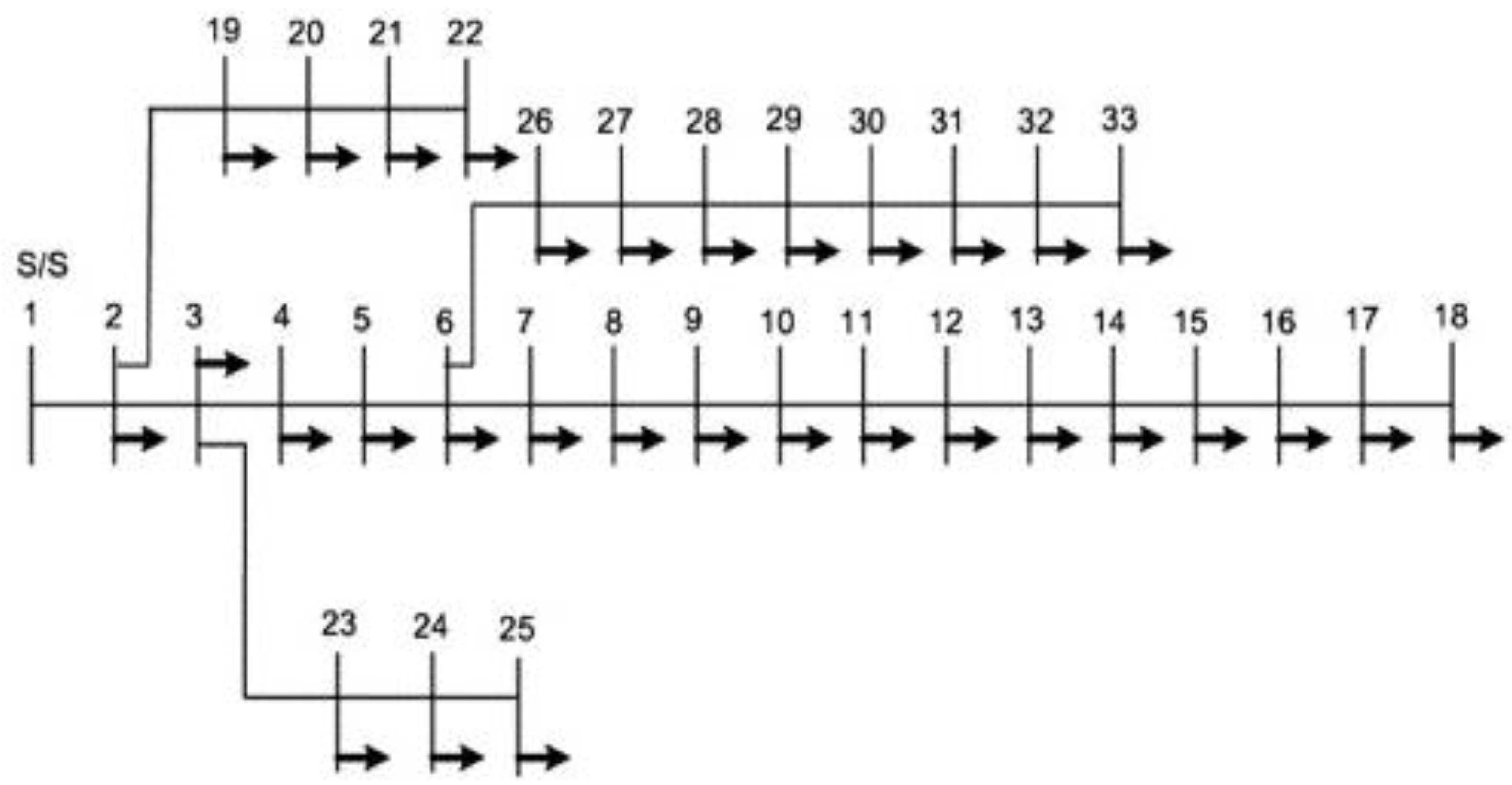
Figure 3.
Harmony Search Algorithm (HSA) flowchart.

Figure 4.
Pseudo code for HSA.

Figure 5.
Effect of load type on voltage profile at 100% loading.
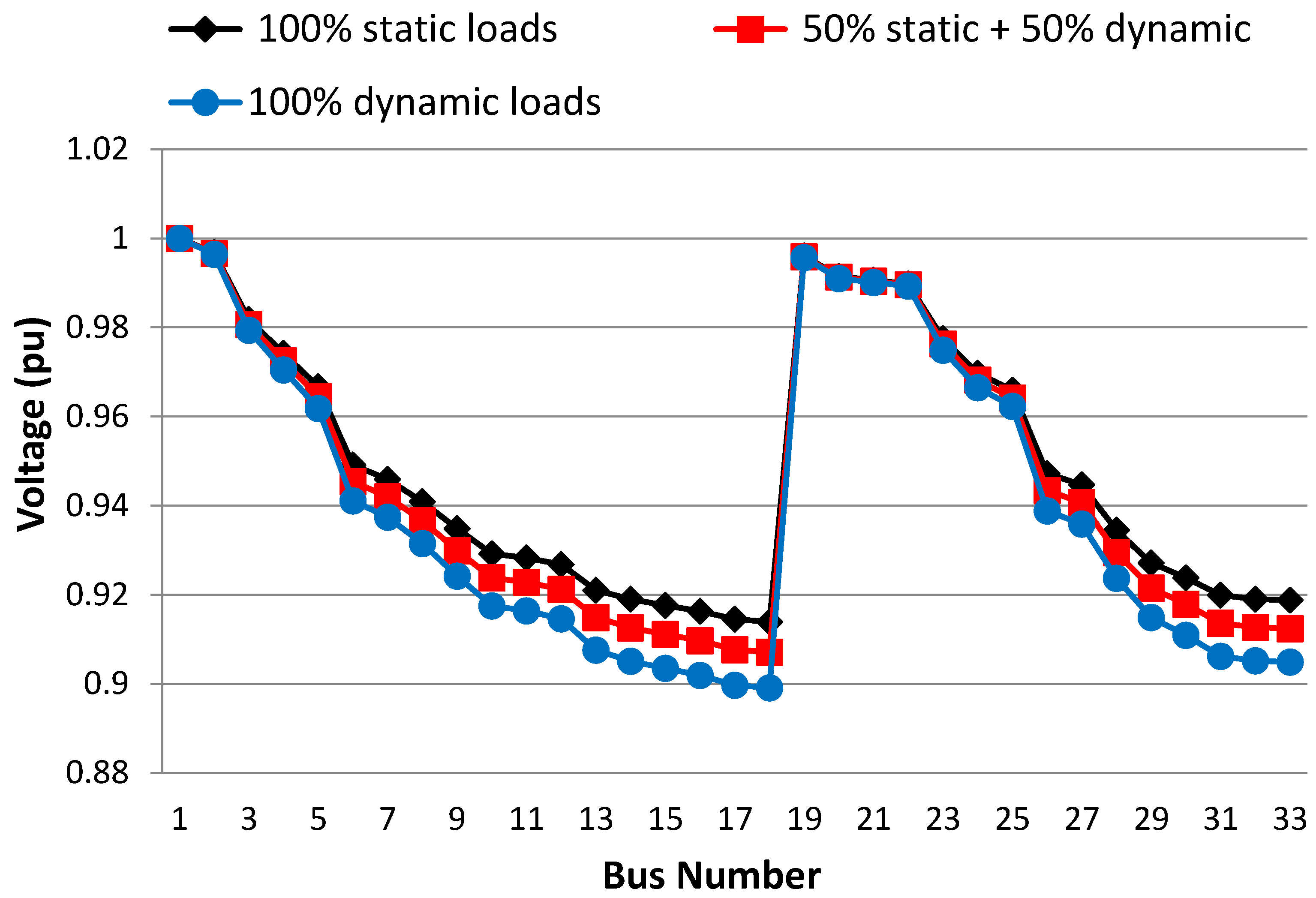
Figure 6.
Effect of load type on voltage profile at 150% loading.

Figure 7.
Effect of load type on voltage profile at 200% loading.
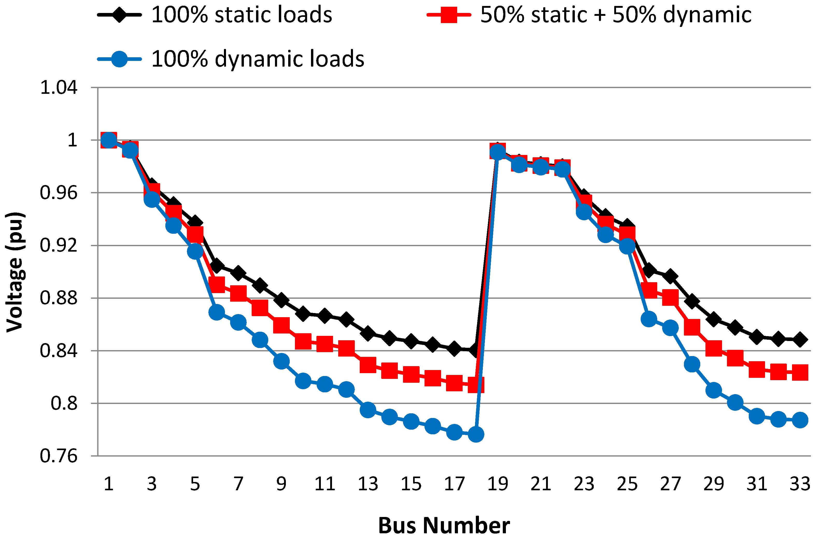
Figure 8.
Effect of load type on voltage profile at 250% loading.

Figure 9.
The voltage profile at 100% loading condition.

Figure 10.
The voltage profile at 150% loading condition.
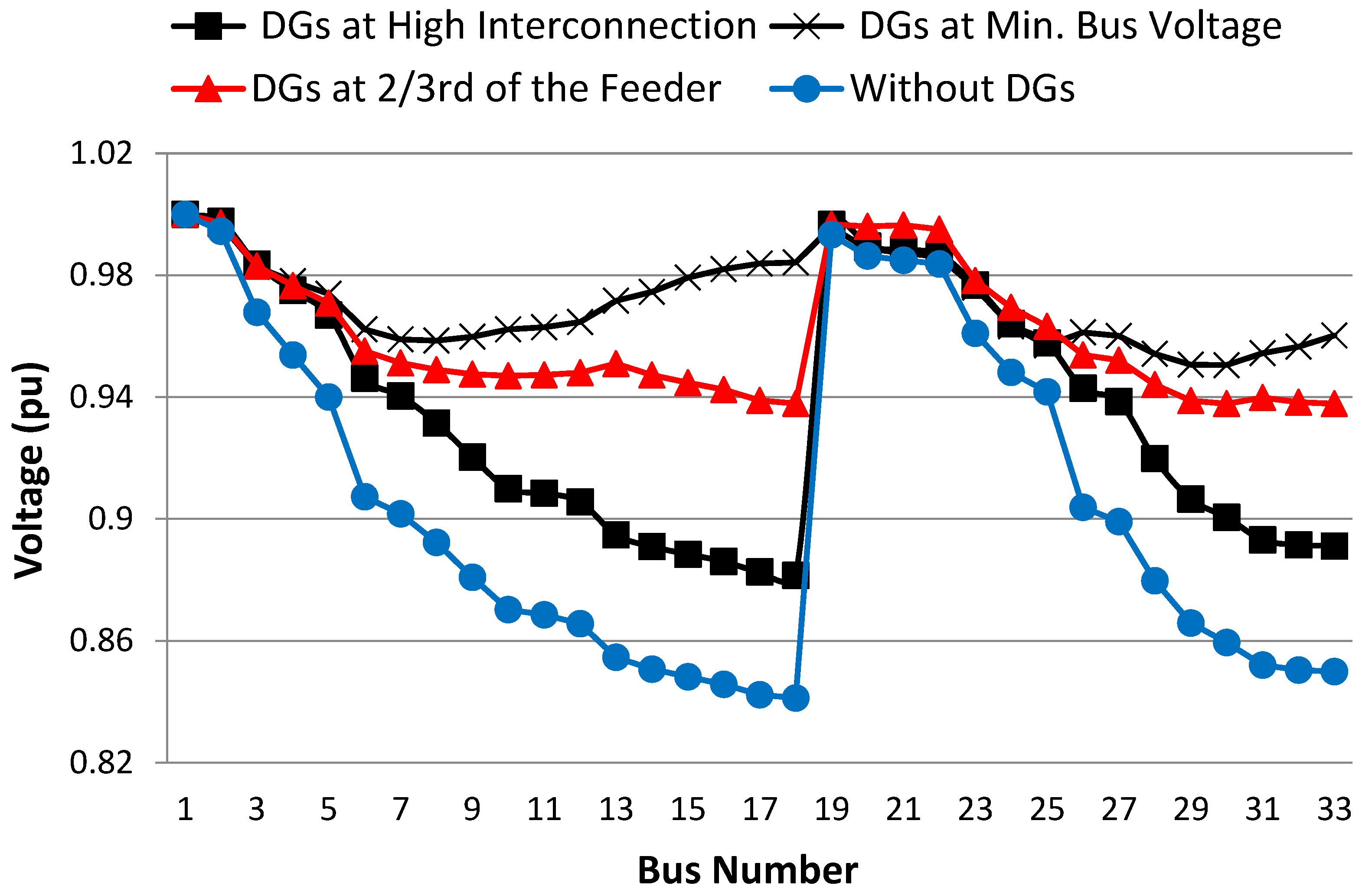
Figure 11.
The voltage profile at 200% loading condition.

Figure 12.
The voltage profile at 250% loading condition.

Figure 13.
The voltage profile at 100% loading condition.
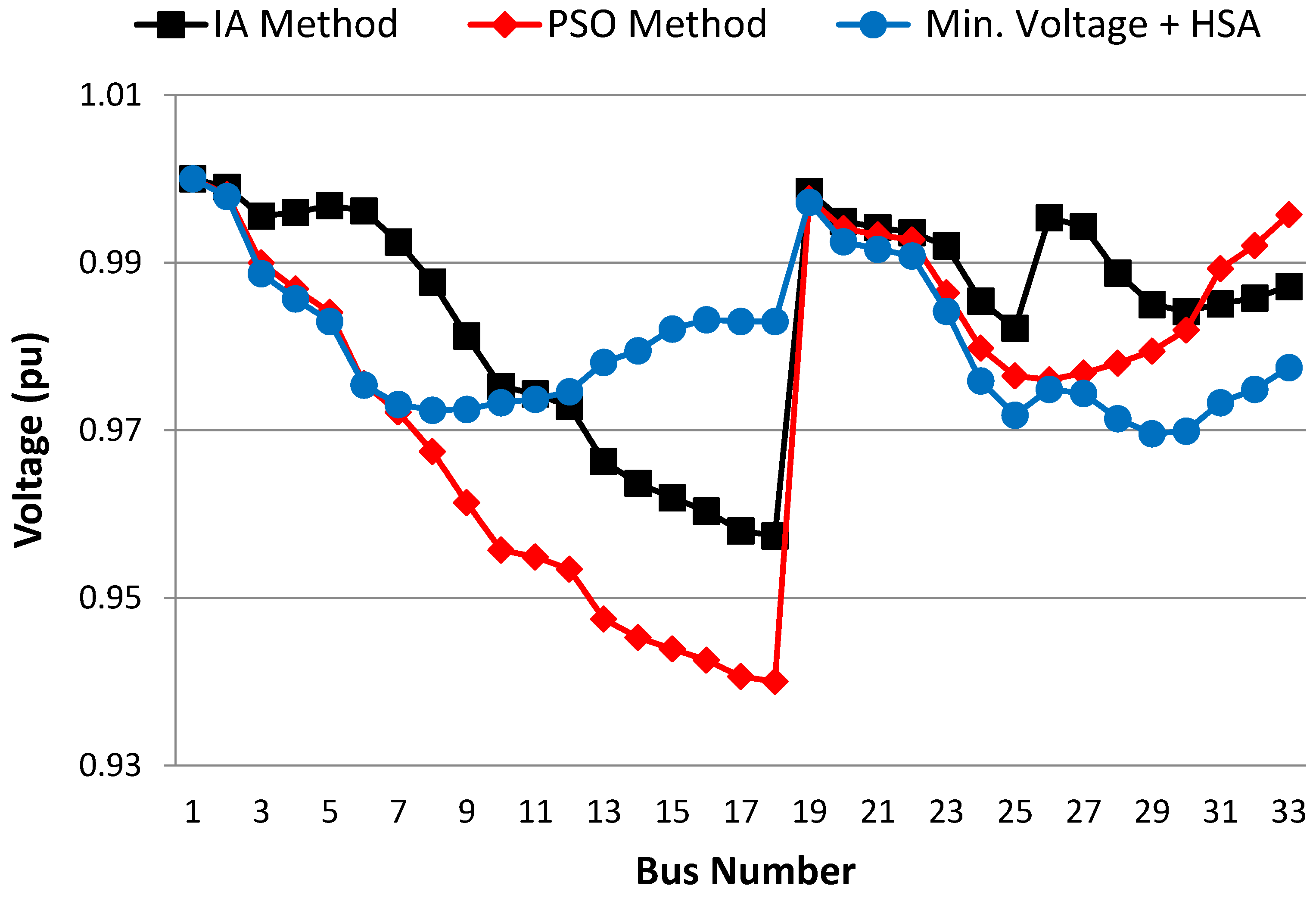
Table 1.
Comparison between static and dynamic loads at 100% loading, i.e., a total load of (3581 + j1745) kVA.
Table 1.
Comparison between static and dynamic loads at 100% loading, i.e., a total load of (3581 + j1745) kVA.
| Case Study at 100% Loading | Min Voltage (pu) | Max Voltage (pu) | Active Power Loss (kW) | Reactive Power Loss (kVAr) |
|---|---|---|---|---|
| 100% static | 0.914 | 1 | 158.10 | 104.53 |
| 50% dynamic + 50% static | 0.907 | 1 | 181.48 | 120.26 |
| 100% dynamic | 0.899 | 1 | 211.01 | 140.17 |
Table 2.
Comparison between static and dynamic loads at 150% loading, i.e., a total load of (5370 + j2617) kVA.
Table 2.
Comparison between static and dynamic loads at 150% loading, i.e., a total load of (5370 + j2617) kVA.
| Case Study 150% Loading | Minimum Voltage (pu) | Max Voltage (pu) | Active Power Loss (KW) | Reactive Power Loss (KVAr) |
|---|---|---|---|---|
| 100% static | 0.876 | 1 | 334.13 | 220.70 |
| 50% dynamic + 50% static | 0.861 | 1 | 411.30 | 272.62 |
| 100% dynamic | 0.841 | 1 | 522.97 | 348.00 |
Table 3.
Comparison between static and dynamic loads at 200% loading, i.e., a total load of (7161 + j3490) kVA.
Table 3.
Comparison between static and dynamic loads at 200% loading, i.e., a total load of (7161 + j3490) kVA.
| Case Study 200% Loading | Minimum Voltage (pu) | Max Voltage (pu) | Active Power Loss (kW) | Reactive Power Loss (kVAr) |
|---|---|---|---|---|
| 100% static | 0.841 | 1 | 559.30 | 369.07 |
| 50% dynamic + 50% static | 0.814 | 1 | 739.37 | 490.23 |
| 100% dynamic | 0.777 | 1 | 1.0446 × 10³ | 696.57 |
Table 4.
Comparison between static and dynamic loads at 250% loading, i.e., a total load of (8950 + j4362) kVA.
Table 4.
Comparison between static and dynamic loads at 250% loading, i.e., a total load of (8950 + j4362) kVA.
| Case Study 250% Loading | Min Voltage (pu) | Max Voltage | Active Power Loss (kW) | Reactive Power Loss (kVAr) |
|---|---|---|---|---|
| 100% static | 0.808 | 1 | 824.7027 | 543.7000 |
| 50% dynamic + 50% static | 0.768 | 1 | 1.1735 × 10³ | 778.4279 |
| 100% dynamic | 0.704 | 1 | 1.8893 × 10³ | 1.2632 × 10³ |
Table 5.
IEEE 33-bus system load flow results for 100% loading without DGs.
| Branch | Active Power Losses (kW) | Reactive Power Losses (kVAr) | Bus | ||
|---|---|---|---|---|---|
| From Bus | To Bus | no. | Voltage (pu) | ||
| 1 | 2 | 13.64 | 6.95 | 1 | 1.000 |
| 2 | 3 | 56.46 | 28.76 | 2 | 0.997 |
| 3 | 4 | 20.60 | 10.49 | 3 | 0.979 |
| 4 | 5 | 19.19 | 9.76 | 4 | 0.971 |
| 5 | 6 | 39.06 | 33.71 | 5 | 0.962 |
| 6 | 7 | 2.12 | 7.01 | 6 | 0.941 |
| 7 | 8 | 5.32 | 1.76 | 7 | 0.937 |
| 8 | 9 | 4.56 | 3.27 | 8 | 0.931 |
| 9 | 10 | 3.86 | 2.73 | 9 | 0.924 |
| 10 | 11 | 0.60 | 0.20 | 10 | 0.916 |
| 11 | 12 | 0.95 | 0.31 | 11 | 0.916 |
| 12 | 13 | 2.88 | 2.26 | 12 | 0.915 |
| 13 | 14 | 0.79 | 1.04 | 13 | 0.908 |
| 14 | 15 | 0.40 | 0.35 | 14 | 0.905 |
| 15 | 16 | 0.31 | 0.23 | 15 | 0.904 |
| 16 | 17 | 0.27 | 0.37 | 16 | 0.902 |
| 17 | 18 | 0.06 | 0.045 | 17 | 0.900 |
| 2 | 19 | 0.21 | 0.20 | 18 | 0.899 |
| 19 | 20 | 1.07 | 0.97 | 19 | 0.996 |
| 20 | 21 | 0.13 | 0.15 | 20 | 0.991 |
| 21 | 22 | 0.06 | 0.07 | 21 | 0.990 |
| 3 | 23 | 3.84 | 2.63 | 22 | 0.989 |
| 23 | 24 | 6.20 | 4.89 | 23 | 0.975 |
| 24 | 25 | 1.54 | 1.21 | 24 | 0.967 |
| 6 | 26 | 2.35 | 1.198 | 25 | 0.962 |
| 26 | 27 | 2.95 | 1.50 | 26 | 0.939 |
| 27 | 28 | 9.78 | 8.62 | 27 | 0.936 |
| 28 | 29 | 6.60 | 5.75 | 28 | 0.924 |
| 29 | 30 | 3.14 | 1.60 | 29 | 0.915 |
| 30 | 31 | 1.83 | 1.82 | 30 | 0.911 |
| 31 | 32 | 0.24 | 0.284 | 31 | 0.906 |
| 32 | 33 | 0.01 | 0.021 | 32 | 0.905 |
| 33 | 0.905 | ||||
Table 6.
Summary of the load flow results at the nominal loading condition (100% loading) or a total connected load of (3581 + j1745) kVA.
Table 6.
Summary of the load flow results at the nominal loading condition (100% loading) or a total connected load of (3581 + j1745) kVA.
| DG Rating | Min. Voltage | Active Power Losses | Reactive Power Losses | |
|---|---|---|---|---|
| DGs at high interconnection | 3000 kW | 0.925 pu | 109.26 kW | 78.86 kVAr |
| DGs at minimum bus voltage | 1686 kW | 0.970 pu | 72.45 kW | 51.55 kVAr |
| DGs at 2/3rd of the feeder [14] | 1685 kW | 0.953 pu | 72.273 kW | 47.71 kVAr |
| Without DGs | ---- | 0.899 pu | 211.01 kW | 140.18 kVAr |
Table 7.
Summary of the load flow results at 150% loading, or a total connected load of (5371.5 + j2617.5) kVA.
Table 7.
Summary of the load flow results at 150% loading, or a total connected load of (5371.5 + j2617.5) kVA.
| DG Rating | Min. Voltage | Active Power Losses | Reactive Power Losses | |
|---|---|---|---|---|
| DGs at high interconnection | 3890 kW | 0.883 | 270.678 kW | 194.078 kVAr |
| DGs at minimum bus voltage | 2491 kW | 0.950 | 169.77 kW | 119.46 kVAr |
| DGs at 2/3rd of the feeder [14] | 2996 kW | 0.938 | 150.43 kW | 100.08 kVAr |
| Without DGs | ---- | 0.841 | 522.97 kW | 348.00 kVAr |
Table 8.
Summary of the load flow results at 200% loading, or a total connected load of (7162 + j3490) kVA.
Table 8.
Summary of the load flow results at 200% loading, or a total connected load of (7162 + j3490) kVA.
| DG Rating | Min. Voltage | Active Power Losses | Reactive Power Losses | |
|---|---|---|---|---|
| DGs at high interconnection | 5033 kW | 0.831 | 543.38 kW | 387.51 kVAr |
| DGs at minimum bus voltage | 3708 kW | 0.953 | 297.15 kW | 217.72 kVAr |
| DGs at 2/3rd of the feeder [14] | 4075 kW | 0.892 | 280.61 kW | 193.40 kVAr |
| Without DGs | ---- | 0.777 | 1045 kW | 696.57 kVAr |
Table 9.
Summary of the load flow results at 250% loading, or a total connected load of (8952 + j4362.5) kVA.
Table 9.
Summary of the load flow results at 250% loading, or a total connected load of (8952 + j4362.5) kVA.
| DG Rating | Min. Voltage | Active Power Losses | Reactive Power Losses | |
|---|---|---|---|---|
| DGs at high interconnection | 6290 kW | 0.777 | 942.23 kW | 672.65 kVAr |
| DGs at minimum bus voltage | 4711 kW | 0.942 | 485.07 kW | 360.92 kVAr |
| DGs at 2/3rd of the feeder [14] | 5302 kW | 0.896 | 403.33 kW | 274.78 kVAr |
| Without DGs | ---- | 0.704 | 1890 kW | 1260 kVAr |
Table 10.
Comparison between the proposed siting and siting of DGs (min. bus voltage + HSA) with other reported techniques in the literature (PSO and IA).
Table 10.
Comparison between the proposed siting and siting of DGs (min. bus voltage + HSA) with other reported techniques in the literature (PSO and IA).
| DG Rating | Min. Voltage | Active Power Losses | Reactive Power Losses | |
|---|---|---|---|---|
| Improved Analytical IA method [25] | 2560.23 kW | 0.9574 | 110.15 kW | ---- |
| PSO method [25] | 1857.5 kW | 0.9400 | 92.44 kW | ---- |
| Minimum bus voltage and HSA | 1686 kW | 0.970 | 72.45 kW | 51.55 kVAr |
Publisher’s Note: MDPI stays neutral with regard to jurisdictional claims in published maps and institutional affiliations. |
© 2022 by the authors. Licensee MDPI, Basel, Switzerland. This article is an open access article distributed under the terms and conditions of the Creative Commons Attribution (CC BY) license (https://creativecommons.org/licenses/by/4.0/).
Share and Cite
MDPI and ACS Style
Sameh, M.A.; Aloukili, A.A.; El-Sharkawy, M.A.; Attia, M.A.; Badr, A.O. Optimal DGs Siting and Sizing Considering Hybrid Static and Dynamic Loads, and Overloading Conditions. Processes 2022, 10, 2713. https://doi.org/10.3390/pr10122713
AMA Style
Sameh MA, Aloukili AA, El-Sharkawy MA, Attia MA, Badr AO. Optimal DGs Siting and Sizing Considering Hybrid Static and Dynamic Loads, and Overloading Conditions. Processes. 2022; 10(12):2713. https://doi.org/10.3390/pr10122713
Chicago/Turabian StyleSameh, Mariam A., Abdulsalam A. Aloukili, Metwally A. El-Sharkawy, Mahmoud A. Attia, and Ahmed O. Badr. 2022. "Optimal DGs Siting and Sizing Considering Hybrid Static and Dynamic Loads, and Overloading Conditions" Processes 10, no. 12: 2713. https://doi.org/10.3390/pr10122713
Note that from the first issue of 2016, this journal uses article numbers instead of page numbers. See further details here.