Elastic Correlative Least-Squares Reverse Time Migration Based on Wave Mode Decomposition

Abstract

The conventional elastic least-squares reverse time migration (LSRTM) generally inverts the parameter perturbation of the model rather than the reflectivity of reflected P- and S-modes, which leads to difficulty in directly interpreting the physical properties of the subsurface media. However, an accurate velocity model that is needed by the separation of seismic records of conventional LSRTM is usually unavailable in real data, which limits its application. In this study, we introduce a new practical correlative LSRTM (CLSRTM) scheme based on wave mode decomposition without amplitude and phase distortion, which frees from separation of seismic records. In this study, we deduced the migration and the de-migration operators using the decoupled P- and S-wave equations in heterogeneous media, which needs no extra wavefield decomposition in simulated data. To accelerate the convergence and improve the efficiency of the inversion, we adopted an analytical step-length formula that can be incidentally computed during the necessary de-migration process and the L-BFGS algorithm. Two numerical examples demonstrate that the proposed method can compensate the energy of deep structures, and generate clear images with balanced amplitudes and enhanced resolution even for the fault structures beneath the salt dome.

1. Introduction

Seismic migration plays an important role in constructing accurate images of the subsurface structure and lithology from seismic data. Compared to ray-tracing based migration and one-way wave equation migration (Claerbout [1]; Claerbout and Doherty [2]; Gazdag [3]; Stoffa et al. [4]; Huang and Fehler [5]), reverse time migration (RTM) (Baysal et al. [6]; McMechan [7]) utilizes a two-way wave equation to propagate the wavefields, which does not suffer from dip limitation and has a higher resolution in complex structures. However, the conventional elastic RTM (ERTM) cannot obtain accurate images due to the assumption of acquisition geometry with regular sampling, infinite acquisition aperture, unbalanced illumination, and unaliased seismic data, which cannot be satisfied in practice (Etgen et al. [8]; Wong et al. [9]). In addition, RTM suffers from low-frequency artifacts generated by cross-correlation between the forward and adjoint wavefields on the wavepath, and the quality of the images depends, for the most part, on the precision of the migration velocity model.

To mitigate the influence of the geometry acquisition problems above, a linear inversion imaging method known as least-squares migration (LSM) (Lambare et al. [10]; Nemeth et al. [11]) has been proposed to improve images. LSM was first applied to Kirchhoff migration (Nemeth et al. [11]; Duquet et al. [12]) and later to one-way wave equation migration (Gazdag [3]), and recently was introduced into RTM (Tang [13]; Dai et al. [14,15]; Wong et al. [9]). For LSM, it aims to find a subsurface reflectivity image that minimizes the L-2 norm of the residuals of observed data and simulated data (generated by Born modeling). In a sense, the key idea of LSM is the amplitude matching strategy.

In general, LSM, especially least-squares RTM (LSRTM), can balance amplitude, mitigate crosstalk of P- and S-modes, and improve the resolution of images. In recent years, many researchers have made great achievements in LSRTM. In 2014, Tan and Huang [16] developed an LSRTM method based on the wavefield-separation imaging condition. In 2015, Wong et al. [9] developed a joint LSRTM scheme to exploit both primaries and free-surface multiples to balance the subsurface illumination. Zhang et al. [17] proposed a new framework for acoustic correlative LSRTM (CLSRTM), which stressed phase information to match the observed data. In 2016, Liu et al. [18] further derived an analytical step-length (ASL) formula for the acoustic CLSRTM. To solve the problem of cycle skipping caused by the large velocity error, Liu and Li [19] developed an LSRTM scheme with an extended imaging condition. In 2014, Dutta and Schuster [20], and Li et al. [21] developed a viscoacoustic LSRTM method to enhance image resolution. In 2015, Sun et al. [22] adopted a constant Q model-based viscoacoustic LSRTM to compensate for attenuation. It is notable that all of the above methods are merely applied to the acoustic case.

The solid Earth is elastic, even viscoelastic and anisotropic, therefore the conventional acoustic approximation-based RTM cannot be directly extended to multicomponent elastic media. Compared with the RTM in acoustic media, multicomponent imaging can provide more attribute information in lithology and geology interpretation, such as sweet-spot detection, fracture prediction, and oil and gas reservoir detection. In addition, the multicomponent can improve the resolution of images due to S-wave being insensitive to the underlying formation and having superiority in imaging steep dip structures. When using an acoustic imaging condition to migrate elastic data, false images may occur. ERTM overcomes this problem and provides reflectivity images of multicomponent data [23,24,25,26]. By comparing PP and PS reflectivity images, one can identify lithology, fractures, fluid/gas, and hydrocarbon reservoirs as the S-wave is more sensitive to fluid/gas phases. Furthermore, the multicomponent images can provide investigation of reservoir attributes, especially in the PS image. However, ERTM suffers from S-wave polarity reversal. For this reason, Dellinger and Etgen [27] developed a Helmholtz decomposition-based ERTM method that uses the divergence and curl operators to separate P- and S-waves. However, this method leads to phase shift and amplitude distortion in S-wave (Sun and McMechan [28]). In this case, some special corrections are needed to obtain an amplitude-preserving image (Sun and McMechan [28]; Sun et al. [29]). Unlike the Helmholtz decomposition, the separated wave equation can decouple the P- and S-waves during propagation, without changing the information of the amplitude and phase in homogeneous media (Ma and Zhu [30]). However, the assumption of homogeneous Lamé parameters is not available in heterogeneous media. In addition, low signal-to-noise (SNR) in seismic records and unbalanced amplitudes lead to a reduction in the SNR of the PS image.

In order to improve the imaging quality based on wave mode separation-based ERTM, elastic LSRTM (ELSRTM) has been proposed to address these issues and can provide high quality images. In 2017, Duan et al. [31] inverted the scalar images of squared P- and S-velocity perturbations based on a new perturbation imaging condition for ELSRTM. Feng and Schuster [32] inverted the reflectivities of P- and S-wave impedance rather than the their velocities or the Lamé parameters as the reflectivities of P- and S-wave impedance are more dissimilar than the Lamé parameters in scattering radiation patterns. In 2018, Rocha et al. [33] derived linearized Born modeling and migration operators based on the energy norm for acoustic and elastic wavefields. Chen et al. [34] inverted P- and S-wave impedance perturbations with pseudo-Hessian preconditioning in ELSRTM. In 2019, Yang et al. [35] utilized an LSRTM scheme based on the subsurface offset domain extended imaging condition to obtain a better resolution when large velocity errors exist. In 2021, Zhong et al. [36] developed a new scheme based on the elastic velocity−stress equation in isotropic media, and inverted reflectivities of P- and S-wave velocity. The above methods chose to invert either velocities, impedances, or Lamé parameters of P- and S-waves, but do not involve density in the inversion process. In 2016, Yang et al. [37] emphasized the importance of involving density variations in LSRTM. In 2017, Qu et al. [38] proposed an ELSRTM method considering the density variations by solving separated velocity−stress elastic wave equations to mitigate the crosstalk due to wave modes coupling, and derived the linearized demigration operator and gradient with respect to P- and S-wave velocities and densities. Chen and Sacchi [39] inverted density, and P- and S-wave velocity perturbation images using the conjugate gradient (CG) method to solve the LSM problem.

Although these ELSRTM methods can obtain high quality images, they invert the model parameter perturbations of the velocity or impedance rather than the reflectivities of P- and S-modes, which cannot generate images with adequate physical meanings, and leads to difficulty in interpreting the subsurface structures. Therefore, based on the separated wave equation, we construct a new framework for elastic CLSRTM (hereafter termed ECLSRTM) to invert the reflectivity of the images, i.e., PP, PS, SP, and SS images. In this paper, we derive the migration operator based on the separated wave equation in heterogeneous media and the de-migration operator without extra wavefield separation of the simulated and observed data. Based on the works of Xiao and Leaney (2010), we only calculated the full wavefield and the S-mode displacement wavefield, then the P-mode component could be obtained by subtracting the latter from the former, thus reducing the cost of computation.

In this paper, we begin with a review of the elastic correlative objective function. Next, we derive the migration and de-migration operators based on the separated wave equation. After that, we present an ASL formula and L-BFGS method to accelerate the convergence rate and improve the efficiency of the inversion. Last, two synthetic examples are presented to demonstrate the effectiveness of the proposed ECLSRTM.

2. Methods

2.1. Correlative Elastic LSRTM

In the CLSRTM, Zhang et al. (2015) proposed a practical and robust cross-correlation-based objective function in acoustic media. We applied it to elastic cases, written as follows,

$$\mathit{E}\left(r\left(\mathit{x}\right)\right)=-{{\displaystyle \iint }}^{ }\frac{{\int }^{ }d\left({\mathit{x}}_r,t|{\mathit{x}}_s\right)·D\left({\mathit{x}}_r,t|{\mathit{x}}_s\right) dt}{\sqrt{{\int }^{ }d\left({\mathit{x}}_r,t|{\mathit{x}}_s\right)·d\left({\mathit{x}}_r,t|{\mathit{x}}_s\right) dt\sqrt{{\int }^{ }D\left({\mathit{x}}_r,t|{\mathit{x}}_s\right)·D\left({\mathit{x}}_r,t|{\mathit{x}}_s\right) dt}}}d{\mathit{x}}_{r}d{\mathit{x}}_s,$$

(1)

where $r\left(x\right)$ is the reflectivity at the position $\mathit{x}$, and $D\left({\mathit{x}}_r,t|{\mathit{x}}_s\right)={\left(u_x,u_z\right)}^T$ and $d\left({\mathit{x}}_r,t|{\mathit{x}}_s\right)={\left(u_x,u_z\right)}^T$ are the observed data and simulated or predicted data, respectively. The objective function of the optimal image can be obtained by minimizing the observed and simulated seismic data to reach its minimum −1 (Zhang et al. [17]). The least-squares (L2) method is an amplitude matching strategy, which is not available in field seismic data due to geometric diffusion and angle effects. Compared to L2, the normalized zero-lag cross-correlation objective function relaxes on the amplitude constraints (is insensitive to differences in amplitude) and utilizes the phase information to measure the similarity of the simulated and observed seismic data.

As for inversion, the problem may be very large, so the efficiency of the optimization algorithm is of great importance. Thus, to solve the optimization problem, gradient-based optimization algorithms are adopted. Usually, the optimization problem needs to be solved efficiently with a tolerable level for both calculation accuracy and the costs of the storage and computations (Wu et al. [40]). In this paper, the nonlinear CG method and the limited memory Broyden−Fletcher−Goldfarb−Shannom (L-BFGS) (Broyden [41]; Fletcher [42]; Goldfrab [43]; Shanno [44]) method are adopted to solve the least-squares optimization problem.

The descent direction of the nonlinear CG method can be written,

$${\mathit{d}}_k=-g_k+{\beta }_k{\mathit{d}}_{k-1},$$

(2)

where ${\mathit{d}}_k$ is the descent direction at $k$-th iteration, $g_k$ is the gradient corresponding to the objective function, and ${\beta }_k$ is a scalar parameter to generate conjugate direction. The scalar parameter ${\beta }_k$ has many variants, Hessian-free CG versions usually including the HS (Hestenes and Stiefel [45]), PRP (Polyak [46]), and CD (Liu and Storey [47]), which are listed as follows,

$${\beta }_k^{HS}=\frac{g_k^T{\mathit{y}}_k}{{\mathit{d}}_{k-1}^T{\mathit{y}}_k},$$

(3a)

$${\beta }_k^{PRP}=\frac{g_k^T{\mathit{y}}_k}{\Vert g_{k-1}\Vert {}^2},$$

(3b)

$${\beta }_k^{CD}=-\frac{\Vert g_k\Vert {}^2}{{\mathit{d}}_{k-1}^T{g}_{k-1}},$$

(3c)

where ${\mathit{y}}_k=g_k-g_{k-1}$, and superscript $T$ means the transpose operator. To guarantee a steady descent of the objective function, the scalar parameter $\beta$ must be greater than zero. However, the scalar parameter calculated by Equation (3a–c) may be less than zero in some special cases, which leads to the opposition of two adjacent search directions. We adopt the following modified scalar parameter,

$${\beta }_k=\mathit{max}\left\{0,\beta \right\},$$

(4)

when $\beta <0$, the CG method will naturally degrade into the steepest descent (SD) method, thus avoiding the opposition of two adjacent search directions.

In contrast, the Newton method has the characteristic of second-order convergence compared to the SD and CG methods, thus having a fast rate of local convergence. However, the computation of the Hessian matrix (second derivatives of objective function) can be extremely expensive. In addition, when the Hessian matrix is nonpositive and ill-conditioned, then additional modification and extra steps are needed. Quasi-Newton methods approximately construct the Hessian inverse matrix without the computation of the full Hessian matrix and its inversion. Here, we focus on the L-BFGS method (Nocedal [48]), which can be expressed as follows,

$${\mathit{d}}_k=-B_k{g}_k,$$

(5)

where $B_k$ is the approximation of the inverse Hessian matrix. The conventional BFGS method calculates the entire elements of $B_k$, which leads to an expensive cost for memory usage. The L-BFGS method calculates the inverse Hessian matrix by only utilizing limited vector sets of $\mathit{y}$ and $\mathit{s}$, without storing the entire Hessian matrix and computing its inversion, where ${\mathit{s}}_k=r_k-r_{k-1}$ is the image perturbation. $B_k$ can be constructed using the vector sets from the last $m$ iterations, where $m$ is an arbitrary number defined by the user. In this paper, we applied the two-loop recursion scheme of the L-BFGS algorithm to compute the descent direction. The initial inverse Hessian matrix is expressed as (Nocedal [48]),

$$B_k^0={\mathit{y}}_k^T{\mathit{s}}_k/{\mathit{y}}_k^T{\mathit{y}}_k,$$

(6)

when the approximation of the inverse Hessian matrix is nonpositive or ill-conditioned, the L-BFGS method fails to construct a sufficient descent direction, thus we restart it using the SD method.

2.2. Decoupled Elastic Wave Equation

ERTM uses elastic full wave equation to calculate the wavefield. In the propagation of wavefield, the P- and S-waves are coupled, which would lead to crosstalk artifacts in imaging and interpretation. Thus, wavefield decomposition is vital in multicomponent imaging. The conventional Helmholtz decomposition-based ERTM (Dellinger and Etgen [27]; Sun and McMechan [28]) separates the compressional P and transverse S components of the wavefield using the divergence and curl of the displacement vector field. However, it distorts the amplitude and phase of the wavefield and generates polarity reversal in an S-wave.

Ma and Zhu [30] proposed a 2D displacement−velocity wave equation based on a separated wave equation to generate vector displacements of P- and S-wave wavefield, without distorting the phase and amplitude. However, the separated elastic wavefields do not convert between the P- and S-waves, and these two wave types decouple when the density and shear modulus are homogeneous (Du et al. [49]).

In this case, Xiao and Leaney [50] proposed the vector displacement equations in heterogeneous media,

$$\rho \ddot{u}=\nabla \left[\left(\lambda +2\mu \right)\nabla ·u\right]-\nabla \times \left(\mu \nabla \times u\right),$$

(7)

where $\rho$ is the density, $\lambda$ and $\mu$ are the Lamé parameters, $u=\left(u_x,u_z\right)$ is the particle displacement, and the double dots above $u$ denote the second-order time derivate. $\nabla =\left({\nabla }_x,{\nabla }_z\right)$, $\nabla ·$, and $\nabla \times$ are the gradient, the divergence, and the curl operators, respectively.

In the work of Xiao and Leaney (2010), they calculated vector displacement equations of the full wavefield, and the P- and S-mode displacement wavefields. To reduce the cost of computation, we only calculated the full wavefield $u$ and the S-mode wavefield $u^{\mathrm{S}}$. The calculation of the P-mode wavefield is written in Equation (9),

$$\rho {\ddot{u}}^{\mathrm{S}}=-\nabla \times \left(\mu \nabla \times u\right),$$

(8)

$$u^{\mathrm{P}}=u-u^{\mathrm{S}}.$$

(9)

The relationship between the Lamé parameters, P-wave velocity $V_{\mathrm{P}}$, and S-wave velocity $V_{\mathrm{S}}$ are written as,

$$\{\begin{array}{l}\lambda =\rho \left(V_{\mathrm{P}}^2-2V_{\mathrm{S}}^2\right)\hfill \\ \mu =\rho V_{\mathrm{S}}^2\hfill \end{array}.$$

(10)

2.3. Reverse Time Migration

ERTM is recognized as an advanced migration tool and is considered to be of high accuracy when imaging the subsurface structures and reflectivities. In heterogeneous media, the 2D multicomponent RTM operator can be written as follows,

$$\{\begin{array}{l}\rho {\ddot{u}}_s\left(\mathit{x},t|{\mathit{x}}_s\right)=\nabla \left[\left(\lambda +2\mu \right)\nabla ·u_s\left(\mathit{x},t|{\mathit{x}}_s\right)\right]-\nabla \times \left[\mu \nabla \times u_s\left(\mathit{x},t|{\mathit{x}}_s\right)\right]\hfill \\ S\left(\mathit{x},t|{\mathit{x}}_s\right)=\delta \left(\mathit{x}-{\mathit{x}}_s\right)f\left(t\right)\hfill \end{array},$$

(11)

where $u_s=\left(u_x,u_z\right)$ is the forward-propagated wavefield with the shot at position ${\mathit{x}}_s, S\left(\mathit{x},t|{\mathit{x}}_s\right)$ is the source function, $\delta$ is the Dirac-delta function, and $f\left(t\right)$ is the source signature. The adjoint state wavefield is written (Zhang and Duan [51]),

$$\{\begin{array}{l}\rho {\ddot{u}}_r\left(\mathit{x},t|{\mathit{x}}_s\right)=\nabla \left[\left(\lambda +2\mu \right)\nabla ·u_r\left(\mathit{x},t|{\mathit{x}}_s\right)\right]-\nabla \times \left[\mu \nabla \times u_r\left(\mathit{x},t|{\mathit{x}}_s\right)\right]\hfill \\ S\left({\mathit{x}}_r,t|{\mathit{x}}_s\right)=-\frac{\partial }{\partial t}\Delta d\left({\mathit{x}}_r,t|{\mathit{x}}_s\right)\delta \left(\mathit{x}-{\mathit{x}}_r\right)\hfill \end{array},$$

(12)

where $u_r=\left(u_x,u_z\right)$ is the backward-propagated receiver wavefield (adjoint wavefield). The adjoint source $\Delta d\left({\mathit{x}}_r,t|{\mathit{x}}_s\right)=\left(\Delta d_x,\Delta d_z\right)$ is expressed as,

$$\Delta d\left({\mathit{x}}_r,t|{\mathit{x}}_s\right)=\frac{1}{\sqrt{{\int }^{ }D·D dt}\sqrt{{\int }^{ }d·d dt}}\left(\frac{{\int }^{ }d·D dt}{{\int }^{ }d·d dt}d-D\right),$$

(13)

2.4. Scalar Imaging Condition for Vector Wavefields

To mitigate crosstalk artifacts generated by P- and S-wave coupling, we adopted the separated wave equation and applied a scalar imaging condition for vector wave modes,

$$r_{\mathrm{PP}}\left(\mathit{x}\right)=\frac{{\iint }^{ }{u}_s^{\mathrm{P}}\left(\mathit{x},t|{\mathit{x}}_s\right)·u_r^{\mathrm{P}}\left(\mathit{x},t|{\mathit{x}}_s\right)dtdx}{{\iint }^{ }{u}_s\left(\mathit{x},t|{\mathit{x}}_s\right)·u_s\left(\mathit{x},t|{\mathit{x}}_s\right)dtdx},$$

(14a)

$$r_{\mathrm{PS}}\left(\mathit{x}\right)=\frac{{\iint }^{ }{u}_s^{\mathrm{P}}\left(\mathit{x},t|{\mathit{x}}_s\right)·u_r^{\mathrm{s}}\left(\mathit{x},t|{\mathit{x}}_s\right)dtdx}{{\iint }^{ }{u}_s\left(\mathit{x},t|{\mathit{x}}_s\right)·u_s\left(\mathit{x},t|{\mathit{x}}_s\right)dtdx},$$

(14b)

$$r_{\mathrm{SP}}\left(\mathit{x}\right)=\frac{{\iint }^{ }{u}_s^{\mathrm{S}}\left(\mathit{x},t|{\mathit{x}}_s\right)·u_r^{\mathrm{P}}\left(\mathit{x},t|{\mathit{x}}_s\right)dtdx}{{\iint }^{ }{u}_s\left(\mathit{x},t|{\mathit{x}}_s\right)·u_s\left(\mathit{x},t|{\mathit{x}}_s\right)dtdx},$$

(14c)

$$r_{\mathrm{SS}}\left(\mathit{x}\right)=\frac{{\iint }^{ }{u}_s^{\mathrm{S}}\left(\mathit{x},t|{\mathit{x}}_s\right)·u_r^{\mathrm{S}}\left(\mathit{x},t|{\mathit{x}}_s\right)dtdx}{{\iint }^{ }{u}_s\left(\mathit{x},t|{\mathit{x}}_s\right)·u_s\left(\mathit{x},t|{\mathit{x}}_s\right)dtdx},$$

(14d)

where $u_s=\left(u_x,u_z\right)$ are the horizontal and vertical components of the source wavefield, $u_s^{\mathrm{P}}=\left(u_{px},u_{pz}\right)$ and $u_s^{\mathrm{S}}=\left(u_{sx},u_{pz}\right)$ are the P- and S-wave modes of the source wavefield, and $u_r^{\mathrm{P}}=\left(u_{px},u_{pz}\right)$ and $u_r^{\mathrm{P}}=\left(u_{px},u_{pz}\right)$ are those of the receiver wavefield, respectively. The symbol $·$ denotes the inner-product operator, and $r_{\mathrm{PP}}$, $r_{\mathrm{PS}}$, $r_{\mathrm{SP}}$, and $r_{\mathrm{SS}}$ are the PP, PS, SP, and SS stacked images, respectively.

In the ECLSRTM scheme, we used Equations (8)–(12) to update the stacked image (Equation (14a–d)). In practice, the SP and SS images have a low resolution for explosive sources, and for this reason, we chose to update PP and PS images in the migration and de-migration processes. In the process of updating the images, we used the initial reflecitivity $r_0\left(\mathit{x}\right)$ calculated by RTM as the input to compute the initial simulated data in the first iteration. Thus, a de-migration operator must be involved accordingly in ECLSRTM. Inspired by the framework of acoustic reverse time de-migration (RTDM) operator derivation (Zhang et al. [17]; Liu et al. [18]), we derived the elastic RTDM operator to generate the multicomponent seismic data.

2.5. Reverse Time Demigration

Zhang and Duan [51] presented the RTDM operator in the acoustic media. In the process of demigration, the Born approximation was used to generate the simulated data based on the reflectivity $r\left(\mathit{x}\right)$. We extended it to the elastic case to predict the simulated seismic data. Firstly, the background wavefield was calculated using the elastic wave of Equation (12). Secondly, we used the reflectivity image $r\left(\mathit{x}\right)$ and source wavefield $u_s\left(\mathit{x},t|{\mathit{x}}_s\right)$ as the input to generate the simulated data $d$, for which the Born approximation is governed by Equation (15). Zhang et al. [17] proved that the demigration operator is the transpose of the migration operator, i.e., forming an adjoint operator pair,

$$\{\begin{array}{l}\rho {\ddot{u}}_r\left(\mathit{x},t|{\mathit{x}}_s\right)=\nabla \left[\left(\lambda +2\mu \right)\nabla ·u_r\left(\mathit{x},t|{\mathit{x}}_s\right)\right]-\nabla \times \left[\mu \nabla \times u_r\left(\mathit{x},t|{\mathit{x}}_s\right)\right]\hfill \\ S\left(\mathit{x},t|{\mathit{x}}_s\right)=r\left(\mathit{x}\right)\frac{\partial u_s\left(\mathit{x},t|{\mathit{x}}_s\right)}{\partial \mathit{x}}\hfill \\ d\left({\mathit{x}}_r,t|{\mathit{x}}_s\right)=u_r\left({\mathit{x}}_r,t|{\mathit{x}}_s\right)\hfill \end{array},$$

(15)

where,

$$r\left(\mathit{x}\right)=r_{\mathrm{PP}}\left(\mathit{x}\right)+r_{\mathrm{PS}}\left(\mathit{x}\right)+r_{\mathrm{SP}}\left(\mathit{x}\right)+r_{\mathrm{SS}}\left(\mathit{x}\right).$$

(16)

Compared to the works of Zhong et al. [36], the proposed demigration operator does not need to separate the observed data, thus it is expected to be applicable to real data, because separating seismic records depend on an accurate velocity. However, an accurate velocity model is usually unavailable in real data. In addition, freeing from separating seismic data decreases the calculation cost and improves the computation efficiency.

In this study, we solved Equations (7), (8), and (15) using a staggered-grid finite difference method.

2.6. Analytical Step Length Formula

To accelerate the convergence, a sufficient descent direction and step length are needed. For local gradient-based optimization problems, an efficient and cost-effective step-length formula is extremely important in this context. Generally, the parabolic search method (PSM; Liu et al. [52]), and the ASL (Liu et al. [18]) formulas are commonly applied. The PSM, a linear search method, involves at least twice as much forward modeling to calculate the optimal step length. Compared with PSM, ASL based on the Taylor expansion of the objective function only calculates the first and second order derivates of $\alpha$ to obtain the optimal step length. Although ASL needs to store the perturbed records of each shot, it involves only one time reading of all seismic records, and can be incidentally calculated during the data prediction process, i.e., during the demigration process, which significantly improves the efficiency of inversion (Liu et al. [18]).

Here, the ASL formula for acoustic CLSRTM based on the linear characteristic of the RTDM operator (Liu et al. [53]) can also be applied to elastic case,

$${\alpha }_{opt}=-\frac{b}{2a},$$

(17)

where,

$$\begin{array}{cc}\hfill a=\frac{1}{2}& {{\displaystyle \iint }}^{ }\frac{1}{\sqrt{{\int }^{ }D·D dt}\sqrt{{\int }^{ }d·d dt}}[2\frac{{\int }^{ }d·\delta d dt}{{\int }^{ }d·d dt}{{\displaystyle \int }}^{ }\delta d·D dt\hfill \\ & \hfill +\frac{{\int }^{ }\delta d·\delta d dt}{{\int }^{ }d·d dt}{{\displaystyle \int }}^{ }d·D dt-3{\left(\frac{{\int }^{ }d·\delta d dt}{{\int }^{ }d·d dt}{{\displaystyle \int }}^{ }d·D dt\right)}^2]d{\mathit{x}}_{r}d{\mathit{x}}_s,\end{array}$$

(18)

and,

$$b={{\displaystyle \iint }}^{ }\frac{1}{\sqrt{{\int }^{ }D·D dt}\sqrt{{\int }^{ }d·d dt}}\left(\frac{{\int }^{ }d·D dt{\int }^{ }d·\delta d dt}{{\int }^{ }d·d dt}-{{\displaystyle \int }}^{ }\delta d·Ddt\right)d{\mathit{x}}_{r}d{\mathit{x}}_s.$$

(19)

In the work of Liu et al. [52], numerical tests proved that the value of the objective function using ASL has a faster convergence rate than PSM. In addition, even for noisy data, the ASL method is more robust, efficient, and accurate in a complex model compared to the PSM. Therefore, we adopted the ASL formula in this paper.

2.7. ECLSRTM Scheme

We assumed that the observed data $D$, the migration velocity of density, and the P- and S-waves are available. The inversion scheme of the proposed ECLSRTM can be summarized as follows,

(1)

Compute initial image $r_{\mathrm{PP}0}\left(\mathit{x}\right)$ and $r_{\mathrm{PS}0}\left(\mathit{x}\right)$ with the observed data $D$ using RTM,

(2)

RTDM to compute the initial simulated data $d_0$ with $r_0$ and misfit $f_0$,

(3)

RTM to compute the two-component gradients $g_{\mathrm{PP}}$ and $g_{\mathrm{PS}}$,

(4)

Update the descent direction ${\mathit{d}}_k=-B_k{g}_k$,

(5)

RTDM to compute the perturbed data $\mathsf{\delta }d$ and the analytical step $\alpha$,

(6)

Update the inverted multicomponent images using $r_{ij}^k=r_{ij}^{k-1}+\delta r_{ij}^k$, where $i,j=\left\{P,S\right\}$ and $k=1, 2,\cdots$ denotes iteration numbers. Simultaneously, update the simulated data using ${\mathit{d}}_k={\mathit{d}}_{k-1}+{\alpha }_k\delta {\mathit{d}}_k$ and compute misfit $f_k$,

(7)

If the misfit is larger than the threshold set by the user, then repeat steps 3 to 6; otherwise, stop this process and output the finial multicomponent images.

3. Numerical Examples

To verify the effectiveness of the proposed ECLSRTM using L-BFGS against the CG method, we present two synthetic examples. The first model is a heterogeneous layered model consist of a sag, while the second model is a complex SEG/SALT model consisting of a salt dome and faults above and beneath the salt dome. In the following two experiments, we give the following stopping criterion. The minimum relative change of the misfit criterion value is set to 0.001 for the layered model, and 0.002 for the SEG/SALT model. The inversion process will exit if the objective function value increases or the relative change of the objective function is less than the misfit criterion set by the user. In numerical experiments, finite difference operator with twelfth-order in space and second-order in time is adopted to improve the precision of forward modeling and the OpenMP multithreads parallel is used to accelerate the calculation for both examples.

3.1. Layered Model

In the first example, a layered model is shown in Figure 1. The layered model consists of 361 × 241 grid cells in the horizontal and vertical directions with a spatial interval of 0.01 km in both directions. In total, 36 shots were fired by a Ricker wavelet, each with a dominant frequency of 15 Hz. Each shot was located at a depth of 0.06 km with an interval of 100 m. The first shot was located at x = 10 m. A maximum of 361 receivers were deployed with fix-spread acquisition geometry and the receivers were fixed at a depth of 0.02 km. The time-sampling interval was 1.0 ms, and the maximum recording time was 2.0 s.

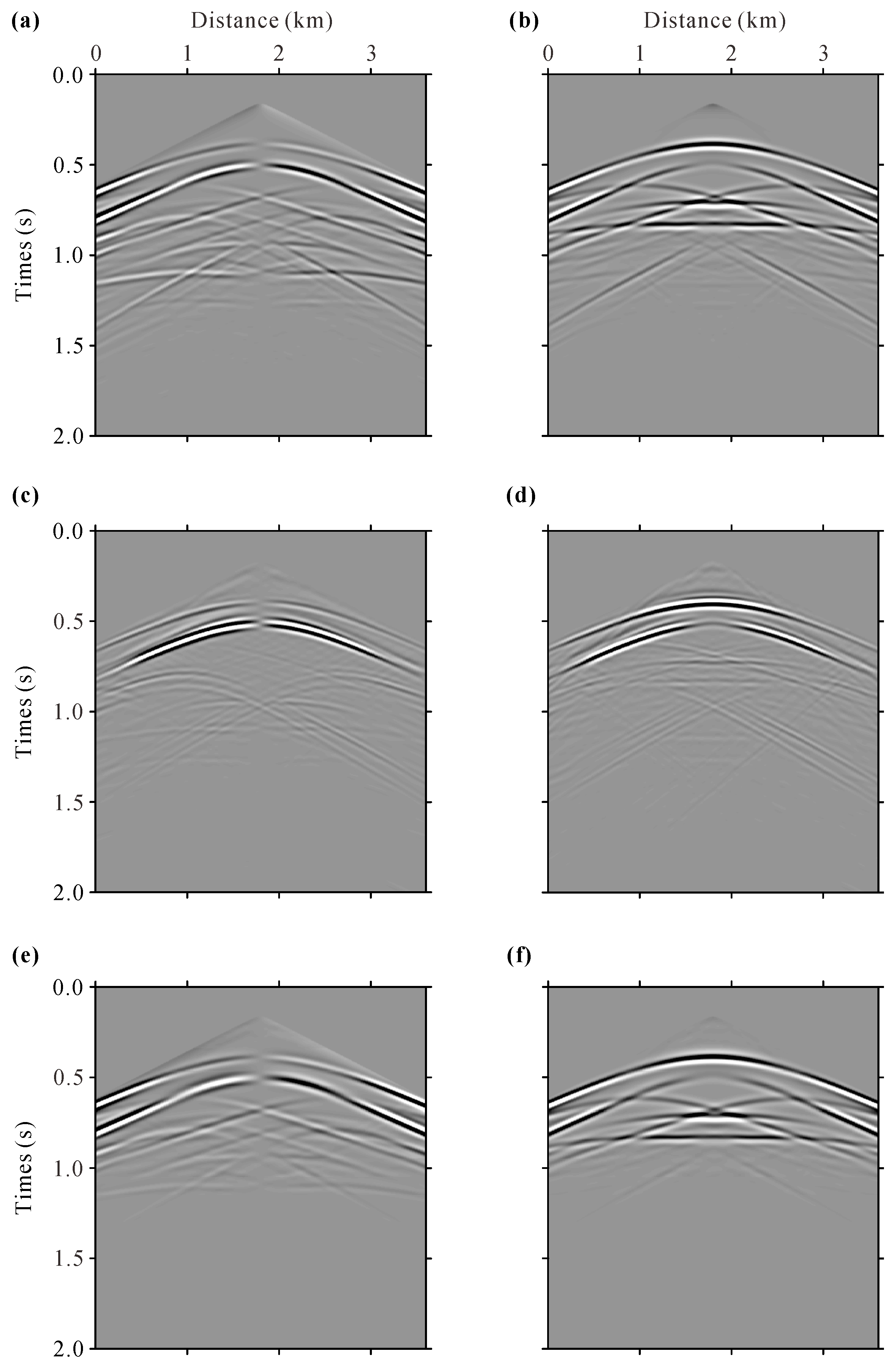
Figure 1 shows the real P- (Figure 1a) and S-wave (Figure 1b) velocity models to generate the synthetic seismic data (observed data), whereas Figure 2 shows those of a Gaussian smoothed version used in the migration. The ERTM images of PP and PS are shown in Figure 3a and Figure 3b, respectively, while those of inverted images generated by ECLSRTM after 20 iterations are shown in Figure 3c and Figure 3d. Compared to the ERTM images, the inverted images have a more balanced amplitude, higher resolution, and less noises.

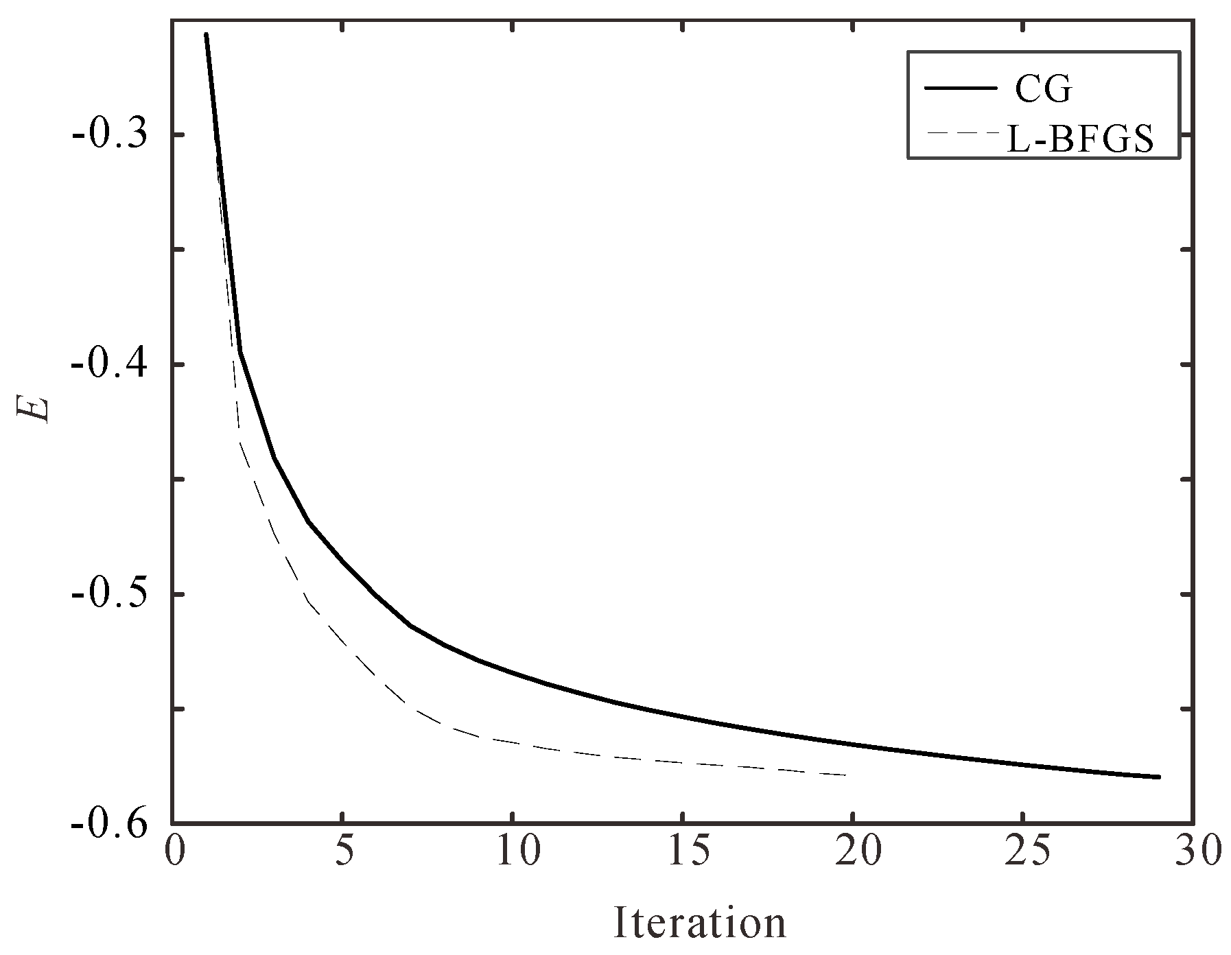
To verify the effectiveness of the L-BFGS method, we adopted the CG and L-BFGS methods for comparison. Figure 4 shows the convergence rate of the CG and L-BFGS methods, respectively. The L-BFGS method exited at the 20-th iteration to reach the criterion value of 0.001, whereas the CG method exited at the 29-th iteration thus demonstrating a lower efficiency.

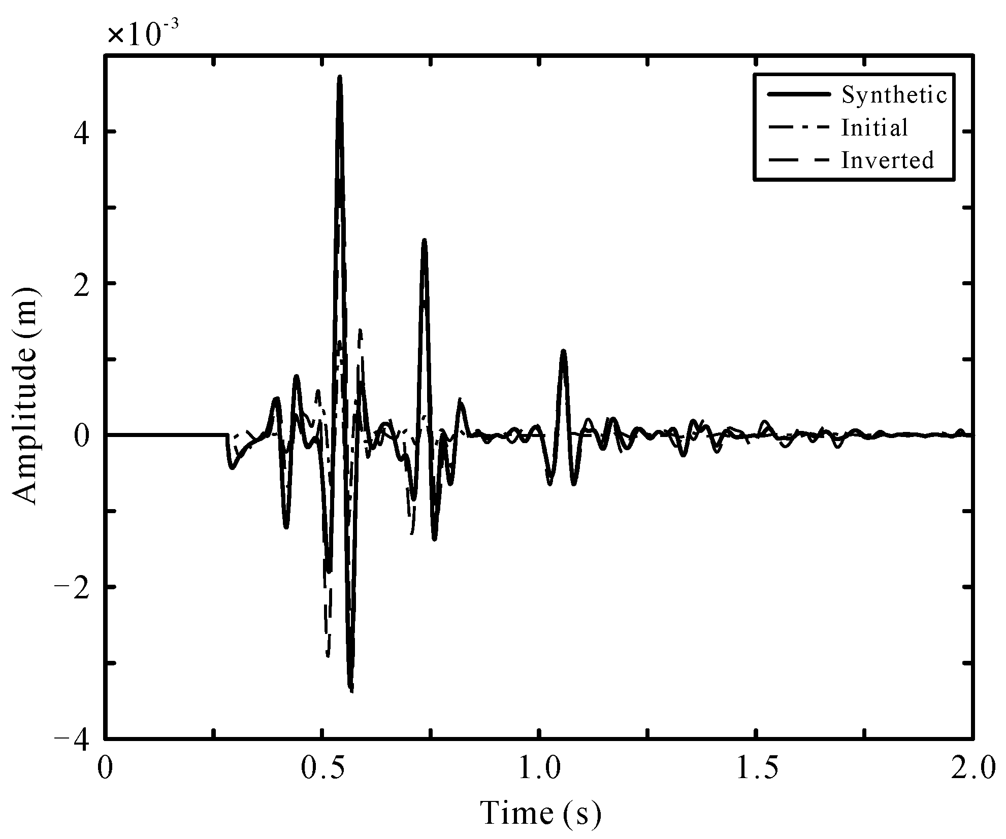
Figure 5a,b shows the horizontal and vertical seismograms of the 19-th synthetic shot with muted direct waves, respectively. Figure 5c and Figure 5d shows the horizontal and vertical components of the initial simulated data calculated with the initial stacked image ${\mathrm{r}}_0$, whereas Figure 5e and Figure 5f shows those of the inverted simulated data generated by ECLSRTM after 20 iterations, respectively. It can be seen that the simulated data calculated by the Born approximation using the inverted images approached the synthetic (observed) data gradually. To verify the similarity between the simulated data and observed data, we extracted traces from the 19-th shot at x = 400 m, as shown in Figure 6. The solid, solid-dotted, and dashed lines denote the synthetic (observed) data, initial data generated by ERTM, and inverted (simulated) data generated by ECLSRTM after 20 iterations, respectively. In Figure 6, it can be observed that the dashed line, i.e., the inverted simulated data generated by the proposed method, matched pretty well with the synthetic record.

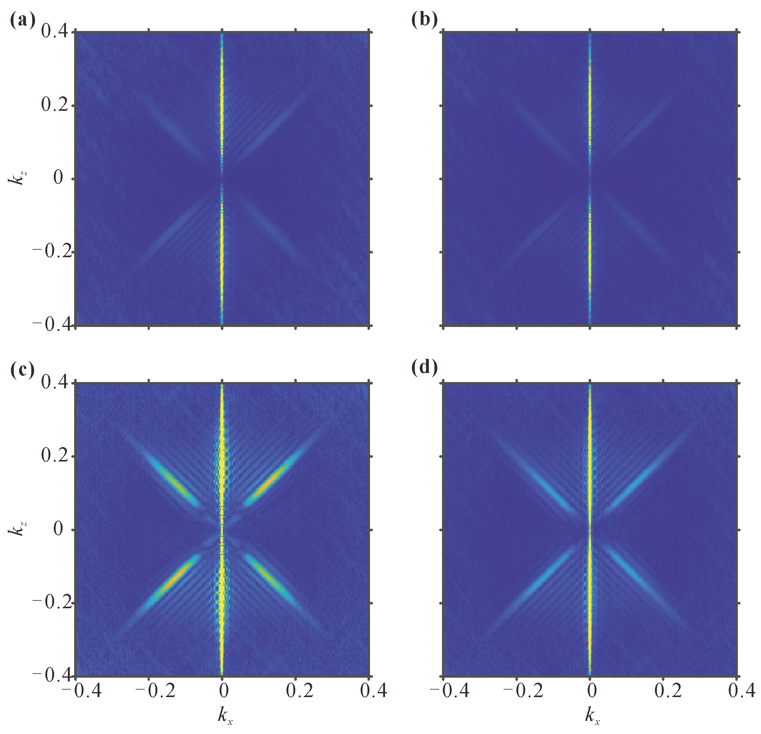
Figure 7a,b shows the wavenumber spectra of the migrated PP and PS image obtained by ERTM, while Figure 7c,d shows those obtained by ECLSRTM, respectively. Compared to the initial ERTM images of PP and PS, the wavenumber spectra of the inverted images after 20 iterations showed higher wavenumber components, which proved the higher resolution of ECLSRTM.

3.2. SEG/SALT Model

The second example involves an application to the SEG/SALT model as shown in Figure 8, while Figure 9 shows those of a Gaussian smooth version used in migration. The subsalt model is manifested as complex subsurface structures and is one of the most challenging problems due to the poor illumination beneath salt bodies. This model consisted of 1290 × 300 grid cells in the horizontal and vertical directions with a 10 m grid spacing in all directions. There were 41 shots in total fired by a Ricker wavelet with a dominant frequency of 15 Hz. Each shot was located at a depth of 0.06 km and was generated with an interval of 0.2 km. The first shot was located at x = 2450 m. The number of receivers was 1290 with a fixed-spread acquisition at the surface. The time-sampling interval was 1.0 ms, and the maximum recording time was 3.5 s.

Figure 10a,b shows the migrated PP and PS images, respectively, while Figure 10c,d shows those generated by ECLSRTM after 18 iterations using the L-BFGS method, respectively. Compared with the initial images generated by ERTM, the inverted images obtained a more balanced amplitude and more even illumination in deep structures, and the shape of the subsalt was sharper, which proved a higher resolution. In particular, it can be seen that the faults pointed out by red arrows exhibited a higher resolution, as shown in Figure 10.

To further verify the efficient convergence rate of the L-BFGS method in the complex model, we analyzed the convergence rate of the CG and L-BFGS methods, as shown in Figure 11. The solid and dashed lines denote the CG and L-BFGS methods, respectively. It can be observed that the convergence curve of the L-BFGS method became flat at the 15th iteration and exited at the 18-th iteration when the relative change of the objective value met the stopping criterion of 0.0002, whereas the curve of the CG method became flat after 25 iterations and exited at the 29-th iteration. This demonstrates that the L-BFGS method is relatively efficient, and can drive the value of the objective function so that it converges to the minimum at a faster rate.

Figure 12a,b shows the horizontal and vertical components of the synthetic data (observed) generated by the real SEG/SALT velocity model, whereas Figure 12c,d shows those of the initial simulated data calculated by the initial stacked image, and Figure 12e,f shows those of the inverted simulated data obtained by ECLSRTM after 18 iterations, respectively. It can be observed that the simulated data obtained by the inverted images approached the observed data gradually.

To verify the similarity between the simulated data and observed data, we extracted traces from the 10-th shot at x = 4250 m, as shown in Figure 13. The solid, solid-dotted, and dashed lines denote the synthetic (observed) data, initial data generated by ERTM, and inverted (simulated) data generated by ECLSRTM after 18 iterations, respectively. Figure 13b shows the zoomed view of the red dashed rectangle in Figure 13a between 0.665 s to 1.025 s. In Figure 13, it can be seen that the dashed line, i.e., the inverted simulated data obtained by the proposed method, matched pretty well with the synthetic (observed) record. It can be observed that the reflected events of the initial seismograms generated by conventional ERTM were weak in the deep structures, while the amplitude of the events of the inverted seismograms generated by the proposed method were more consistently even in both horizontal and vertical directions.

To further verify the improvement of the resolution, we calculated the wavenumber spectra of the PP and PS images, as shown in Figure 14. Figure 14a,b shows the wavenumber spectra of the initial PP and PS images generated by ERTM, while Figure 14c,d shows those of the inverted images obtained by ECLSRTM after 18 iterations, respectively. Compared with traditional ERTM, we verified that the wavenumber spectra of the inverted images had higher wavenumber components, thus improving the resolution of the inverted images.

4. Discussion

In contrast with the inversion schemes of impedance, P- and S-wave velocity models, and other forms of elastic parameters, we chose to invert the reflectivity images, which represent physical meanings in geological interpretations. We deduced the de-migration operator that needs no separation of seismic records in comparison with works of the conventional ELSRTM of multicomponent seismic data, which reduce the cost of computation and remove the accurate velocity model dependence required by the separation of seismic records.

As shown by Zhang et al. (2015) and Liu et al. (2016), CLSRTM is expected to be more practical and robust than the amplitude-matching-based LSRTM. It relaxes the amplitude matching and stresses the phase information approximate for the observed seismic data. However, it shares the common shortcomings of LSRTM, i.e., the accuracy of the migration velocity model, when compared to ray theory-based LSM, such as the Kirchhoff least-squares migration. We will further test its potential application in real data.

5. Conclusions

We developed a new inversion scheme for the ECLSRTM method for multicomponent seismic data to obtain reflectivity images. Inversion for the reflectivity rather than parameter perturbations has physical meanings in interpreting the physical properties of the subsurface media. Compared with alternative ELSRTM methods, the proposed ECLSRTM method relaxes on the amplitude matching and uses phase constraints, which are expected to be robust. Synthetic examples show that our ECLSRTM improved the image quality, obtained a higher resolution, balanced the amplitude, and compensated for illumination. Based on the linear characteristic of a pair of operators, we derived both the migration and de-migration operators of the ECLSRTM in heterogeneous media. The de-migration operator only requires the reflectivity images of PP and PS to generate the simulated data, without extra calculations of the decomposition of the P- and S-mode wavefields compared with the conventional ELSRTM. Furthermore, we applied the ASL formula and the L-BFGS method for ECLSRTM to accelerate the convergence rate. As can be seen in the numerical tests, the L-BFGS method is more efficient in that it can derive the value of the objective function value to the minimum. In addition, compared with the conventional LSRTM (Gu et al., 2019), our scheme removes the requirement of the separation of seismic records that depends on an accurate velocity model. However, an accurate velocity model is usually unavailable, which further verifies that our method is more practical. Therefore, the presented method is expected to be applicable to real data.

References

- Claerbout, J. Toward a unified theory of reflector mapping. Geophysics 1971, 36, 467–481. [Google Scholar] [CrossRef]
- Claerbout, J.; Doherty, S. Downward continuation of moveout corrected seismograms. Geophysics 1972, 37, 741–768. [Google Scholar] [CrossRef] [Green Version]
- Gazdag, J. Wave equation migration with the phase-shift method. Geophysics 1978, 43, 1342–1351. [Google Scholar] [CrossRef]
- Stoffa, P.L.; Fokkema, J.T.; Freire, R.M.D.; Kessinger, W.P. Split step Fourier migration. Geophysics 1990, 55, 410–421. [Google Scholar] [CrossRef]
- Huang, L.J.; Fehler, M.C. Accuracy analysis of the split-step Fourier propagator: Implications for seismic modeling and migration. Bull. Seismol. Soc. Am. 1998, 88, 18–29. [Google Scholar] [CrossRef]
- Baysal, E.; Kosloff, D.; Sherwood, J. Reverse time migration. Geophysics 1983, 48, 1514–1524. [Google Scholar] [CrossRef] [Green Version]
- McMechan, G.A. Migration by extrapolation of time-dependent boundary values. Geophys. Prospect. 1983, 31, 413–420. [Google Scholar] [CrossRef]
- Etgen, J.; Gray, S.H.; Zhang, Y. An overview of depth imaging in exploration geophysics. Geophysics 2009, 74, WCA5–WCA17. [Google Scholar] [CrossRef]
- Wong, M.; Biondi, B.L.; Ronen, S. Imaging with primaries and free-surface multiples by joint least-squares reverse time migration. Geophysics 2015, 80, S223–S235. [Google Scholar] [CrossRef]
- Lambaré, G.; Virieux, J.; Madariaga, R.; Jin, S. Iterative asymptotic inversion in the acoustic approximation. Geophysics 1992, 57, 1138–1154. [Google Scholar] [CrossRef]
- Nemeth, T.; Wu, C.; Schuster, G.T. Least-squares migration of incomplete reflection data. Geophysics 1999, 64, 208–221. [Google Scholar] [CrossRef]
- Duquet, B.; Marfurt, K.J.; Dellinger, J.A. Kirchhoff modeling inversion for reflectivity and subsurface illumination. Geophysics 2000, 65, 1195–1209. [Google Scholar] [CrossRef]
- Tang, Y. Target-oriented wave-equation least-squares migration/inversion with phase-encoded Hessian. Geophysics 2009, 74, WCA95–WCA107. [Google Scholar] [CrossRef] [Green Version]
- Dai, W.; Wang, X.; Schuster, G.T. Least-squares migration of multisource data with a deblurring filter. Geophysics 2011, 76, R135–R146. [Google Scholar] [CrossRef]
- Dai, W.; Fowler, P.; Schuster, G.T. Multi-source least-squares reverse time migration. Geophys. Prospect. 2012, 60, 681–695. [Google Scholar] [CrossRef]
- Tan, S.R.; Huang, L.J. Least-squares reverse-time migration with a wavefield-separation imaging condition and updated source wavefields. Geophysics 2014, 79, S195–S205. [Google Scholar] [CrossRef]
- Zhang, Y.; Duan, L.; Xie, Y. A stable and practical implementation of least-squares reverse time migration. Geophysics 2015, 80, V23–V31. [Google Scholar] [CrossRef]
- Liu, Y.S.; Teng, J.W.; Xu, T.; Bai, Z.M.; Lan, H.Q.; Badal, J. An efficient step-length formula for correlative least-squares reverse time migration. Geophysics 2016, 81, S221–S238. [Google Scholar] [CrossRef] [Green Version]
- Liu, Y.; Li, Z. Least-squares reverse-time migration with extended imaging condition. Chin. J. Geophys. 2015, 58, 3771–3782. [Google Scholar]
- Dutta, G.; Schuster, G.T. Attenuation compensation for least-squares reverse time migration using the viscoacoustic-wave equation. Geophysics 2014, 79, S251–S262. [Google Scholar] [CrossRef] [Green Version]
- Li, Z.; Guo, Z.; Tian, K. Least-squares reverse time migration in visco-acoustic medium. Chin. J. Geophys. 2014, 57, 214–228. [Google Scholar]
- Sun, J.; Fomel, S.; Zhu, T. Preconditioning least-squares RTM in viscoacoustic media by Q-compensated RTM. In Proceedings of the SEG Technical Program Expanded Abstracts, New Orleans, LA, USA, 18 October 2015; pp. 3959–3964. [Google Scholar]
- Liu, Q.C.; Zhang, J.F.; Zhang, H. Eliminating the redundant source effects from the cross-correlation reverse-time migration using a modified stabilized division. Comput. Geosci. 2016, 92, 49–57. [Google Scholar] [CrossRef]
- Liu, Q.C. Dip-angle image gathers computation using poynting vector in elastic reverse-time migration and their application for noise suppression. Geophysics 2019, 84, S159–S169. [Google Scholar] [CrossRef]
- Liu, Q.C.; Zhang, J.F. Topography least-squares reverse-time migration based on adaptive unstructured mesh. Surv. Geophys. 2019, 41, 343–361. [Google Scholar] [CrossRef]
- Li, Z.Y.; Liu, Y.S.; Liang, G.H.; Xue, G.Q.; Wang, R.J. First-order particle velocity equations of decoupled P-and S-wavefields and their application in elastic reverse time migration. Geophysics 2021, 86, S387–S404. [Google Scholar] [CrossRef]
- Dellinger, J.; Etgen, J. Wavefield separation in two-dimensional anisotropic media. Geophysics 1990, 55, 914–919. [Google Scholar] [CrossRef]
- Sun, R.; McMechan, G.A. Scalar reverse-time depth migration of prestack elastic seismic data. Geophysics 2001, 66, 1519–1527. [Google Scholar] [CrossRef]
- Sun, R.; McMechan, G.A.; Chuang, H. Amplitude balancing in separating P- and S-waves in 2D and 3D elastic seismic data. Geophysics 2011, 76, S103–S113. [Google Scholar] [CrossRef]
- Ma, D.T.; Zhu, G.M. Numerical modeling of P-wave and S-wave separation in elastic wavefield. OGP 2003, 38, 482–486. [Google Scholar]
- Duan, Y.T.; Guitton, A.; Sava, P. Elastic least-squares reverse time migration. Geophysics 2017, 82, S315–S325. [Google Scholar] [CrossRef] [Green Version]
- Feng, Z.C.; Schuster, G.T. Elastic least-squares reverse time migration. Geophysics 2017, 82, S143–S157. [Google Scholar] [CrossRef] [Green Version]
- Rocha, D.; Sava, P.; Guitton, A. 3D acoustic least-squares reverse time migration using the energy norm. Geophysics 2018, 83, S261–S270. [Google Scholar] [CrossRef]
- Chen, K.; Sacchi, M.D. Elastic least-squares reverse time migration via linearized elastic full waveform inversion with pseudo-Hessian preconditioning. Geophysics 2017, 82, S341–S358. [Google Scholar] [CrossRef] [Green Version]
- Yang, J.Z.; Li, Y.Y.E.; Cheng, A.; Liu, Y.Z.; Dong, L.G. Least-squares reverse time in the presence of velocity errors. Geophysics 2019, 84, S567–S580. [Google Scholar] [CrossRef]
- Zhong, Y.; Gu, H.M.; Liu, Y.T.; Mao, Q.H. Elastic least-squares reverse time migration based on decoupled wave equations. Geophysics 2021, 86, S371–S386. [Google Scholar] [CrossRef]
- Yang, J.Z.; Liu, Y.Z.; Dong, L.G. Least-squares reverse time migration in the presence of density variations. Geophysics 2016, 81, S497–S509. [Google Scholar] [CrossRef]
- Qu, Y.M.; Li, J.L.; Huang, J.P.; Li, Z.C. Elastic least-squares reverse time migration with velocities and density perturbation. Geophys. J. Int. 2017, 212, 1033–1056. [Google Scholar] [CrossRef] [Green Version]
- Chen, K.; Sacchi, M.D. The importance of including density in elastic least-squares reverse time migration: Multiparameter crosstalk and convergence. Geophys. J. Int. 2018, 261, 61–80. [Google Scholar] [CrossRef]
- Wu, S.J.; Wang, Y.B.; Zheng, Y.K.; Chang, X. Limited memory BFGS based least-squares pre-stack Kirchhoff depth migration. Geophys. J. Int. 2015, 202, 738–747. [Google Scholar] [CrossRef]
- Broyden, C.G. The convergence of a class of double-rank minimization algorithms. J. Inst. Math. Appl. 1970, 6, 76–90. [Google Scholar] [CrossRef]
- Fletcher, R. A new approach to variable metric algorithms. Comput. J. 1970, 13, 317–322. [Google Scholar] [CrossRef] [Green Version]
- Goldfarb, D. A family of variable metric updates derived by variational means. Math. Comput. 1970, 24, 23–26. [Google Scholar] [CrossRef]
- Shanno, D.F. Conditioning of quasi-Newton methods for function minimization. Math. Comput. 1970, 24, 647–656. [Google Scholar] [CrossRef]
- Hestenes, M.R.; Stiefel, E.L. Methods of conjugate gradients for solving linear systems. J. Res. Natl. Bur. Stand. 1952, 5, 409–436. [Google Scholar] [CrossRef]
- Polyak, B.T. The conjugate gradient method in extreme problems. USSR Comput. Math. Math. Phys. 1969, 9, 94–112. [Google Scholar] [CrossRef]
- Liu, Y.; Storey, C. Efficient generalized conjugate gradient algorithms, part1: Theory. J. Optim. Theory Appl. 1991, 69, 129–137. [Google Scholar] [CrossRef]
- Nocedal, J. Updating quasi-Newton matrices with limited storage. Math. Comput. 1980, 95, 339–353. [Google Scholar] [CrossRef]
- Du, Q.Z.; Guo, C.F.; Zhao, Q.; Gong, X.F.; Wang, C.X.; Li, X.Y. Vector-based elastic reverse time migration based on scalar imaging condition. Geophysics 2017, 82, S111–S127. [Google Scholar] [CrossRef]
- Xiao, X.; Leaney, W.S. Local vertical seismic profiling (VSP) elastic reverse-time migration and migration resolution: Salt-flank imaging with transmitted P-to-S waves. Geophysics 2010, 75, S35–S49. [Google Scholar] [CrossRef]
- Zhang, Y.; Duan, L. Predicting multiples using a reverse time demigration. In Proceedings of the 83rd Annual International Meeting, SEG, Expanded Abstracts, Las Vegas, NV, USA, 4–9 November 2012; pp. 520–524. [Google Scholar]
- Liu, Y.S.; Teng, J.W.; Xu, T.; Badal, J.; Liu, Q.Y.; Zhou, B. Effects of conjugate gradient methods and step-length formulas on the multiscale full waveform inversion in time domain: Numerical experiments. Pure Appl. Geophys. 2017, 174, 1983–2006. [Google Scholar] [CrossRef]
- Liu, Y.S.; Teng, J.W.; Xu, T.; Wang, Y.H.; Liu, Q.Y.; Badal, J. Robust time-domain full waveform inversion with normalized zero-lag cross-correlation objective function. Geophys. J. Int. 2016, 209, 106–112. [Google Scholar] [CrossRef] [Green Version]
Figure 1.
The real layered velocity model: (a) Density; (b) P-wave velocity; (c) S-wave velocity.
Figure 2.
The smoothed layered velocity model: (a) Density; (b) P-wave velocity; (c) S-wave velocity.
Figure 3.
Migration images of the layered model: (a) PP image of ERTM; (b) PS image of ERTM; (c) PP image of ECLSRTM after 20 iterations using L-BFGS; (d) PS image of ECLSRTM after 20 iterations using L-BFGS.
Figure 4.
Convergence of the objective function in the case of the layered model. Solid and dashed lines denotes the result in reference to CG and L-BFGS, respectively.
Figure 5.
The 19-th shot records (direct waves are muted) of the layered model: (a) Horizontal component of synthetic data; (b) Vertical component of synthetic data; (c) Horizontal component of simulated data using ERTM; (d) Vertical component of simulated data using ERTM; (e) Horizontal component of simulated data using ECLSRTM after 20 iterations; (f) Vertical component of simulated data using ECLSRTM after 20 iterations.
Figure 6.
Traces extracted from the 19-th shot of the layered model at x = 400 m.
Figure 7.
Wavenumber spectra of images in the case of the layered model: (a) Initial PP image using ERTM; (b) Initial PS image using ERTM; (c) Inverted PP image using ECLSRTM after 20 iterations; (d) Inverted PS image using ECLSRTM after 20 iterations.
Figure 8.
The real SEG/SALT velocity model: (a) Density; (b) P-wave velocity; (c) S-wave velocity.
Figure 9.
The smoothed SEG/SALT velocity model: (a) Density; (b) P-wave velocity; (c) S-wave velocity.
Figure 10.
Migration images of the SEG/SALT model: (a) PP image of ERTM; (b) PS image of ERTM; (c) PP image of ECLSRTM after 18 iterations using L-BFGS; (d) PS image of ECLSRTM after 18 iterations using L-BFGS.
Figure 11.
Convergence of the objective function in the case of the SEG/SALT model. Solid and dashed lines denote the results in reference to CG and L-BFGS, respectively.
Figure 12.
The 10-th shot records (direct waves are muted) of the SEG/SALT model: (a) Horizontal component of synthetic data; (b) Vertical component of synthetic data; (c) Horizontal component of simulated data using ERTM; (d) Vertical component of simulated data using ERTM; (e) Horizontal component of simulated data using ECLSRTM after 18 iterations; (f) Vertical component of simulated data using ECLSRTM after 18 iterations.
Figure 13.
Traces extracted from the 10-th shot at x = 4250 m. Solid, solid-dotted, and dashed lines denote the synthetic (observed) data, initial data generated by ERTM, and inverted (simulated) data generated by ECLSRTM after 18 iterations, respectively: (a) Traces extracted from the 10-th shot at x = 4250 m; (b) Zoomed view of the Figure 13a in the red dashed region from time 0.665 s to 1.025 s.
Figure 14.
Wavenumber spectra of the images in the case of the SEG/SALT model: (a) Initial PP image using ERTM; (b) Initial PS image using ERTM; (c) Inverted PP image using ECLSRTM after 18 iterations; (d) Inverted PS image using ECLSRTM after 18 iterations.
Publisher’s Note: MDPI stays neutral with regard to jurisdictional claims in published maps and institutional affiliations. |
© 2022 by the authors. Licensee MDPI, Basel, Switzerland. This article is an open access article distributed under the terms and conditions of the Creative Commons Attribution (CC BY) license (https://creativecommons.org/licenses/by/4.0/).
Share and Cite
MDPI and ACS Style
Zheng, Y.; Liu, Y.; Xu, T.; Li, Z. Elastic Correlative Least-Squares Reverse Time Migration Based on Wave Mode Decomposition. Processes 2022, 10, 288. https://doi.org/10.3390/pr10020288
AMA Style
Zheng Y, Liu Y, Xu T, Li Z. Elastic Correlative Least-Squares Reverse Time Migration Based on Wave Mode Decomposition. Processes. 2022; 10(2):288. https://doi.org/10.3390/pr10020288
Chicago/Turabian StyleZheng, Yue, Youshan Liu, Tao Xu, and Zhiyuan Li. 2022. "Elastic Correlative Least-Squares Reverse Time Migration Based on Wave Mode Decomposition" Processes 10, no. 2: 288. https://doi.org/10.3390/pr10020288
Note that from the first issue of 2016, this journal uses article numbers instead of page numbers. See further details here.