Optimization Control Strategy for a Central Air Conditioning System Based on AFUCB-DQN

Abstract

The central air conditioning system accounts for 50% of the building energy consumption, and the cold source system accounts for more than 60% of the total energy consumption of the central air conditioning system. Therefore, it is crucial to solve the optimal control strategy of the cold source system according to the cooling load demand, and adjust the operating parameters in time to achieve low energy consumption and high efficiency. Due to the complex and changeable characteristics of the central air conditioning system, it is often difficult to achieve ideal results using traditional control methods. In order to solve this problem, this study first coupled the building cooling load simulation environment and the cold source system simulation environment to build a central air conditioning system simulation environment. Secondly, noise interference was introduced to reduce the gap between the simulated environment and the actual environment, and improve the robustness of the environment. Finally, combined with deep reinforcement learning, an optimal control strategy for the central air conditioning system is proposed. Aiming at the simulation environment of the central air conditioning system, a new model-free algorithm is proposed, called the dominant function upper confidence bound deep Q-network (AFUCB-DQN). The algorithm combines the advantages of an advantage function and an upper confidence bound algorithm to balance the relationship between exploration and exploitation, so as to achieve a better control strategy search. Compared with the traditional deep Q-network (DQN) algorithm, double deep Q-network (DDQN) algorithm, and the distributed double deep Q-network (D3QN) algorithm, the AFUCB-DQN algorithm has more stable convergence, faster convergence speed, and higher reward. In this study, significant energy savings of 21.5%, 21.4%, and 22.3% were obtained by conducting experiments at indoor thermal comfort levels of 24 °C, 25 °C, and 26 °C in the summer.

1. Introduction

With the rapid development of the global economy, building energy consumption is increasing, and has become one of the three major energy-consuming sectors, alongside industrial and transportation energy consumption. In office buildings that utilize central air conditioning, the energy consumption of central air conditioning accounts for approximately 50% of the total building energy consumption [1]. The energy consumption of the chiller system constitutes 60% to 80% of the entire air conditioning system [2]. Most central air conditioning systems operate with parameters set to their maximum values, making the optimization of chiller system operating parameters crucial for energy savings in the overall central air conditioning system. The cooling load of building air conditioning is influenced by various factors, such as outdoor meteorological parameters, building design, and indoor occupancy. Therefore, dynamically controlling the system’s operating parameters based on cooling load demand to improve energy efficiency has typically been a focal point in research on energy savings in central air conditioning systems [3]. Table 1 presents the key findings from recent research articles in the field.

Since the introduction of adaptive algorithms in 1980, adaptive control has become one of the important means to solve the problem of adjusting control parameters of air conditioning systems [4]. In the context of the European Union (EU) and governments around the world developing mandatory building energy research and conservation policies for buildings and their air conditioning systems [5], it has become crucial to properly establish the energy performance of buildings and their different systems to reduce the gap between building energy model (BEM) simulation results and actual measurements [6]. The core of central air conditioning energy-saving optimal control is to find the best air conditioning control parameters while maintaining indoor comfort requirements to achieve the goal of minimum energy consumption. Gao et al. [7] proposed an event-triggered distributed model predictive control (DMPC) scheme for improving indoor temperature regulation in multizone buildings. By comprehensively considering energy consumption and thermal comfort, the scheme determines the optimal temperature set point and verifies its effectiveness in practical cases. Sampath et al. [8] controlled the heating, ventilation, and air conditioning (HVAC) system through an adaptive control system, which improved the thermal comfort of the occupants and the system efficiency. Giuseppe et al. [9] proposed an optimization framework based on model predictive control and genetic algorithms to minimize heating energy costs and thermal discomfort. Yang et al. [10] successfully reduced the total energy consumption of the air conditioning water system by using the improved parallel artificial immune system (IPAIS) algorithm. Sun et al. [11] used the equilibrium optimization (EO) algorithm to optimize the load scheduling of chillers in the HVAC system, which effectively saved energy consumption. Tang et al. [12] proposed a model predictive control (MPC) method for optimally controlling central air conditioning systems integrated with cold storage during rapid demand response (DR) events, achieving power reduction and indoor environment optimization, reducing energy consumption, and ensuring comfort. However, central air conditioning systems are highly nonlinear, uncertain, time-varying, and coupled, which increase the requirements for control algorithms. Traditional adaptive algorithms and control methods often fail to achieve ideal control effects when dealing with these challenges [13]. In addition, the mechanism modeling and parameter identification of these algorithms are relatively complex.

Reinforcement learning (RL) [14] is a machine learning approach that has emerged in recent years, and is characterized by self-learning and online learning capabilities. Through the mechanism of “actions and rewards”, RL can achieve the adaptive optimization of controllers in the absence of control system models, making it a data-driven control method. Deep reinforcement learning (DRL) [15] inherits the feature representation capabilities of deep learning and the ability of reinforcement learning to interact autonomously with the environment. In recent years, DRL has been widely applied in the field of air conditioning control, and can be categorized into model-based and model-free RL. Model-based methods refer to the Markov decision process (MDP) five-tuple (state S, reward R, action A, state transition probability P, discount factor gamma). If the five-tuple is fully known, it is considered a model-based method; otherwise, it is regarded as a model-free method.

Model-based algorithms are appealing for task implementation because an optimized model can provide the intelligent agent with “foresight” to simulate scenarios and understand the consequences of actions, even in the absence of knowledge about the dynamic environment. Monte Carlo tree search (MCTS) is the most well-known model-based algorithm widely applied in many board games, such as chess and Go. The iterative linear quadratic regulator (iLQR) [16] and MPC generally require stringent assumptions to be made for their implementation. Zhao et al. [17] proposed a model-based DRL approach using a hybrid model to address the heating, ventilation, and air conditioning control problem, which improved learning efficiency and reduced learning costs. Chen et al. [18] combined model-based deep reinforcement learning with MPC to propose a novel learning-based control strategy for HVAC systems, demonstrating the effectiveness of the algorithm through simulation experiments. However, acquiring an accurate model is challenging for most problems. Many environments are stochastic, and their dynamic transitions are unknown, requiring the model to be learned. Modeling in environments with large state and action spaces is particularly difficult, especially when the transitions are complex. Furthermore, the model can only be effective if it can accurately predict future changes in the environment. In particular, central air conditioning systems, as complex multivariable systems, pose additional challenges in modeling and prediction.

Model-free RL learns optimal control strategies by interacting with the model-free building environment, avoiding cumbersome modeling work [19] and offering better scalability and generalization capabilities [20]. For instance, Heo et al. [21] proposed a data-driven intelligent ventilation control strategy based on deep reinforcement learning, effectively improving system performance through deep Q-network (DQN) algorithm-controlled air conditioning systems. Yuan et al. [22] presented a reinforcement learning-based control strategy for a variable air volume (VAV) air conditioning system. Wei et al. [23] introduced a data-driven approach based on deep reinforcement learning to control variable air volume HVAC systems. Deng et al. [24] combined active building environment change detection with DQN to propose a novel HVAC control strategy, effectively saving energy consumption. Lei et al. [25] proposed a practical person-centric multivariable HVAC control framework based on DRL, utilizing a branching dueling Q-network (BDQ) to significantly reduce energy consumption. Marantos et al. [26] applied neural network-fitted Q-iteration methods to HVAC system control, achieving significant improvements in energy efficiency and thermal comfort compared to rule-based controllers. Zhang et al. [27] used the asynchronous advantage actor–critic (A3C) algorithm to control HVAC systems, making them suitable for the overall building energy model and achieving energy-saving effects. Wang et al. [28] applied the Monte Carlo actor–critic algorithm with long short-term memory (LSTM) neural networks to HVAC system control to achieve optimization effects. Ding et al. [29] proposed a deep reinforcement learning-based multizone residential HVAC thermal comfort control strategy, implementing the optimal HVAC thermal comfort control policy through a deep deterministic policy gradient (DDPG). Zhang et al. [30] reduced the heating demand in office building heating systems through deep reinforcement learning training. Gao et al. [31] developed a DDPG-based method to learn the optimal thermal comfort control policy, effectively reducing HVAC energy consumption.

Table 1. Summary of previous research papers and their contributions.

Approach	Reference	Contributions
traditional algorithm	[7]	The proposed DMPC scheme can reduce the energy consumption of multizone buildings and improve the thermal comfort of occupants.
	[8]	Higher air conditioning system performance and energy efficiency can be achieved through adaptive control systems.
	[9]	Through an optimization framework of model predictive control and genetic algorithms, significant energy savings can be achieved in the coldest and highest energy cost situations while maintaining comfort.
	[10]	Improved parallel artificial immune system algorithm reduces system energy consumption.
	[11]	Successfully optimized the load distribution of chillers in the HVAC system using a balance optimization algorithm, achieving energy savings.
	[12]	An MPC approach is proposed to optimize the operation of central air conditioning systems with integrated cold energy storage during rapid demand response (DR) events.
Deep reinforcement learning (model-based)	[17]	A hybrid model-based deep reinforcement learning approach is proposed for HVAC system control.
	[18]	Proposed model-based deep reinforcement learning and model predictive control (MBRL-MC), a novel learning control strategy combining model predictive control and deep reinforcement learning, for HVAC systems.
Deep reinforcement learning (model-free)	[21]	An intelligent ventilation control system based on the deep reinforcement learning algorithm is proposed, which achieves the goal of real-time control of indoor air quality and energy saving.
	[22]	Used RL algorithms to optimize air conditioning system operation, save energy efficiently, and perform well in multizone air supply.
	[23]	A data-driven DRL approach was developed for intelligently scheduling a building’s HVAC system, reducing energy consumption.
	[24]	A novel approach to HVAC control is proposed, utilizing active environmental change detection and deep Q-networks.
	[25]	A practical deep reinforcement learning (DRL) approach is proposed for multivariable, occupant-centric HVAC system control.
	[26]	A decision-making mechanism is proposed to support the smart thermostat task using reinforcement learning techniques.
	[27]	A deep reinforcement learning framework for optimal control of HVAC systems utilizing a whole building energy model is proposed.
	[28]	A reinforcement learning-based controller is proposed to optimize HVAC systems in buildings using long short-term memory neural networks.
	[29]	A method for the thermal comfort control of multizone residential HVAC systems based on deep reinforcement learning is proposed.
	[30]	A practical control framework based on deep reinforcement learning (BEM-DRL) is proposed for the application of a building energy model (BEM) in real-time HVAC optimal control.
	[31]	A framework DeepComfort based on deep reinforcement learning is proposed for thermal comfort and energy-saving control of buildings.

Table 1. Summary of previous research papers and their contributions.

Approach	Reference	Contributions
traditional algorithm	[7]	The proposed DMPC scheme can reduce the energy consumption of multizone buildings and improve the thermal comfort of occupants.
	[8]	Higher air conditioning system performance and energy efficiency can be achieved through adaptive control systems.
	[9]	Through an optimization framework of model predictive control and genetic algorithms, significant energy savings can be achieved in the coldest and highest energy cost situations while maintaining comfort.
	[10]	Improved parallel artificial immune system algorithm reduces system energy consumption.
	[11]	Successfully optimized the load distribution of chillers in the HVAC system using a balance optimization algorithm, achieving energy savings.
	[12]	An MPC approach is proposed to optimize the operation of central air conditioning systems with integrated cold energy storage during rapid demand response (DR) events.
Deep reinforcement learning (model-based)	[17]	A hybrid model-based deep reinforcement learning approach is proposed for HVAC system control.
	[18]	Proposed model-based deep reinforcement learning and model predictive control (MBRL-MC), a novel learning control strategy combining model predictive control and deep reinforcement learning, for HVAC systems.
Deep reinforcement learning (model-free)	[21]	An intelligent ventilation control system based on the deep reinforcement learning algorithm is proposed, which achieves the goal of real-time control of indoor air quality and energy saving.
	[22]	Used RL algorithms to optimize air conditioning system operation, save energy efficiently, and perform well in multizone air supply.
	[23]	A data-driven DRL approach was developed for intelligently scheduling a building’s HVAC system, reducing energy consumption.
	[24]	A novel approach to HVAC control is proposed, utilizing active environmental change detection and deep Q-networks.
	[25]	A practical deep reinforcement learning (DRL) approach is proposed for multivariable, occupant-centric HVAC system control.
	[26]	A decision-making mechanism is proposed to support the smart thermostat task using reinforcement learning techniques.
	[27]	A deep reinforcement learning framework for optimal control of HVAC systems utilizing a whole building energy model is proposed.
	[28]	A reinforcement learning-based controller is proposed to optimize HVAC systems in buildings using long short-term memory neural networks.
	[29]	A method for the thermal comfort control of multizone residential HVAC systems based on deep reinforcement learning is proposed.
	[30]	A practical control framework based on deep reinforcement learning (BEM-DRL) is proposed for the application of a building energy model (BEM) in real-time HVAC optimal control.
	[31]	A framework DeepComfort based on deep reinforcement learning is proposed for thermal comfort and energy-saving control of buildings.

In recent years, research has primarily focused on proposing energy-saving strategies for HVAC systems using deep reinforcement learning methods and validating the performance of these algorithms. However, there is still insufficient research on energy-saving strategies for cooling systems and improving deep reinforcement learning algorithms to adapt to these strategies. Additionally, stable and secure data obtained from real-world central air conditioning system environments are scarce, and the cost of data acquisition is high, making it unsuitable for directly training reinforcement learning agents. Therefore, it is necessary to establish a simulated environment for central air conditioning systems that closely resembles real-world conditions.

This research considered multiple factors that influence building cooling loads, including solar radiation, human heat dissipation, heat transfer through external windows, and heat transfer through exterior walls, to construct a simulation environment for building cooling loads. For the chiller unit, cooling tower, and water pump, this research established a simulation environment for the cooling source system. By coupling the simulation environment for the building cooling load with the simulation environment for the cooling source system, this research created a simulated environment for the central air conditioning system. To make the simulation environment more realistic in terms of data collection processes for operating parameters, this research introduced noise interference and, consequently, enhanced the robustness of the environment. This approach not only allows the simulation of data anomalies caused by various disturbances, but also improves the reliability of the simulation environment.

For the established simulated environment of the central air conditioning system, this research proposes the advantaged upper confidence bound deep Q-network (AFUCB-DQN) algorithm. Unlike traditional DQN algorithms, this research utilized an advantage function to reduce the influence of air conditioning data variance on environmental variance. This research also combined the upper confidence bound (UCB) algorithm to address the issue of sampling errors caused by environmental stochasticity induced by noise. The main contributions of this paper are summarized as follows:

• This research proposes a comprehensive simulation environment for deep reinforcement learning that considers the building cooling load, which can provide guidance for the energy optimization of real-world central air conditioning systems.
• This research took into account various disturbances encountered during sensor data collection of the cooling source system in real-world environments. To reduce the discrepancy between the constructed simulation environment and the real environment, and enhance the robustness of the environment, this research introduced noise interference.
• For the proposed simulation environment of the central air conditioning system in this paper, this research introduced an advantage function based on the DQN algorithm and combined it with the UCB algorithm to form the proposed AFUCB-DQN algorithm.

The remaining sections of this paper are organized as follows. Section 2 presents the theoretical background of reinforcement learning, the Q-learning algorithm, and the DQN algorithm. Section 3 constructs and couples the simulation environment for building cooling load with the simulation environment for the cooling source system, while establishing the Markov decision process for the central air conditioning system. Section 4 introduces the proposed AFUCB-DQN algorithm. Section 5 validates the simulation environment and discusses the experimental results. Section 6 summarizes the paper and proposes directions for future work.

2. Related Theory

This section introduces the relevant theory of reinforcement learning, Q-learning, and DQN algorithms. The main terms used in this paper are summarized in Table 1.

2.1. Reinforcement Learning

The reinforcement learning process can be represented by Figure 1 [32], which is a system composed of an environment and an agent. The environment generates information describing the system state, referred to as states. The agent observes the states and uses this information to select actions and interact with the environment. The environment accepts the actions and transitions to the next state, then it returns the next state and a reward to the agent. When the (state → action → reward) loop is completed, one time step is finished. By continually repeating this process, the environment eventually terminates, obtaining the optimal policy for a specific task and maximizing the cumulative expected return.

2.2. Q-Learning

The Q-learning algorithm [33] is a classic model-free algorithm that involves constructing a Q-table that stores the expected rewards (Q-value) for different actions in each state–action pair. In this algorithm, the agent selects actions based on the current state by choosing the state with the maximum Q-value. The Q-value represents the estimation of the current reward plus the discounted future rewards, and serves as an approximation of the reward function.

The Q-learning algorithm is not constrained by the environment model or the state transition function, as it accumulates experience through interactions with the environment. Convergence of the Q-table is achieved when the values in the table no longer undergo significant changes. The updated formula for the state–action value function in this algorithm is as follows:

$$\mathrm{Q}\left(\mathrm{s}, \mathrm{a}\right)=\mathrm{Q}\left(\mathrm{s}, \mathrm{a}\right)+\mathsf{\alpha }\left(\mathrm{r}+\mathsf{\gamma }\underset{{\mathrm{a}}_{\mathrm{t}+1}}{\max }\mathrm{Q}\left({\mathrm{s}}_{\mathrm{t}+1}{, \mathrm{a}}_{\mathrm{t}+1}\right) - \mathrm{Q}\left(\mathrm{s}, \mathrm{a}\right)\right)$$

(1)

In this context, the reward discount factor γ ∈ [0, 1] represents the extent to which current actions influence future rewards. When γ equals 0, the agent only considers immediate rewards [34]. The Q-learning algorithm learns by continuously updating the Q-table. However, frequent read and write operations on Q-values can decrease learning efficiency and limit the algorithm’s capability to handle larger state spaces.

2.3. DQN

The DQN combines the advantages of the Q-learning algorithm with deep neural networks to enhance its ability to handle large state spaces [35]. The DQN algorithm uses a deep neural network as a function approximator, consisting of two parts: the action network and the target network. Initially, the action network and the target network have the same parameter settings. During the training process, the parameters of the action network are updated through training. However, after a certain number of steps (N steps), the DQN algorithm copies the parameters of the action network to the target network for parameter updates. In each iteration, the DQN algorithm randomly selects a small batch of samples $\left({\mathrm{s}}_{\mathrm{t}}{, \mathrm{a}}_{\mathrm{t}}{, \mathrm{r}}_{\mathrm{t}}{, \mathrm{s}}_{\mathrm{t}+1}\right)$ from the experience replay buffer, with ${\mathrm{s}}_{\mathrm{t}+1}$ as the input of the action network, which outputs the Q-values for each action at state ${\mathrm{s}}_{\mathrm{t}}$, denoted as $\mathrm{Q}\left(\mathrm{s}, \mathrm{a}, \mathsf{\omega }\right)$, where $\mathsf{\omega }$ represents the parameters of the neural network. During training, the weights of the action network are updated by solving the target values. When computing the target values, the state ${\mathrm{s}}_{\mathrm{t}+1}$ is input into the target network, which outputs the maximum Q-value for each action at state ${ \mathrm{s}}_{\mathrm{t}+1}$, denoted as $\underset{\mathrm{a}+1}{\max }\mathrm{Q}\left({\mathrm{s}}_{\mathrm{t}+1}{, \mathrm{a}}_{\mathrm{t}+1}, \mathsf{\omega }\right)$.

In the DQN algorithm, the loss function is constructed as shown in the following formula:

$$\mathrm{L}\left(\mathsf{\omega }\right)=\mathrm{E}\left[{\left(\mathrm{r}+\mathsf{\gamma }\underset{\mathrm{a}+1}{\max }\mathrm{Q}\left({\mathrm{s}}_{\mathrm{t}+1}{, \mathrm{a}}_{\mathrm{t}+1}, \mathsf{\omega }\right) - \mathrm{Q}\left(\mathrm{s}, \mathrm{a}, \mathsf{\omega }\right)\right)}^2\right]$$

(2)

Taking the partial derivative of the loss function with respect to the parameters $\mathsf{\omega }$, we obtain the next gradient and update the network parameters $\mathsf{\omega }$.

$$\frac{\mathsf{\delta }\mathrm{L}\left(\mathsf{\omega }\right)}{\mathsf{\delta }\mathsf{\omega }}=\left[\mathrm{r}+\left(\mathsf{\gamma }\underset{\mathrm{a}+1}{\max }\mathrm{Q}\left({\mathrm{s}}_{\mathrm{t}+1}{, \mathrm{a}}_{\mathrm{t}+1}, \mathsf{\omega }\right) - \mathrm{Q}\left(\mathrm{s}, \mathrm{a}, \mathsf{\omega }\right)\right)\right]\frac{\mathsf{\delta }\mathrm{Q}\left(\mathrm{s}, \mathrm{a}, \mathsf{\omega }\right)}{\mathsf{\delta }\mathsf{\omega }}$$

(3)

During the training process, the DQN algorithm incorporates an experience replay mechanism, which breaks the correlations between samples and enhances the stability of the algorithm. Additionally, the DQN algorithm constrains the range of reward values and error terms, ensuring that the Q-values and gradient values remain within reasonable bounds, further improving the stability of the algorithm.

3. Environment Construction

In this study, this article carried out the coupling of building cooling load simulation environment and cold source system simulation environment, in order to realize the comprehensive simulation and control optimization of central air conditioning system. Specifically, this research established a building cooling load simulation environment that can consider outdoor meteorological conditions and building characteristics, including temperature, humidity, solar radiation, and building parameters, to accurately calculate the building’s cooling load demand. At the same time, this research also established a cold source system simulation environment to simulate the operating status of the chiller system.

In order to realize the coupling between the building cooling load and the cooling source system, this research applied the output of the building cooling load simulation environment as the input of the cooling source system simulation environment. Specifically, the building cooling load simulation environment provides real-time cooling load demand information to the cold source system simulation environment, and the cold source system simulation environment adjusts the operating parameters of the chiller according to this demand information, including chilled water supply temperature, chilled water flow, cooling water flow, and cooling tower air volume. In this way, the cold source system can be dynamically adjusted according to the actual demand of the building’s cooling load, so as to optimize energy consumption and improve energy saving effects. Through the above coupled methods, this research realized the comprehensive simulation and control optimization of the central air conditioning system. This integrated approach can more accurately simulate the operation of the central air conditioning system, and provide guidance for the optimal control of the actual central air conditioning system.

In order to keep the indoor temperature stable, this research designed the cooling capacity of the air conditioner to be 1.2 times the cooling load of the building, so as to provide enough cooling capacity reserve to meet the demands of sudden temperature fluctuations and load increases. Furthermore, in order to optimize the control parameters of the cold source system, this research modeled the simulated environment of the central air conditioning system as a Markov decision process, and used a deep reinforcement learning algorithm for training and convergence. Through this modeling method, the system can learn and output the best control action, so that the cold source system can be optimized and controlled according to the actual situation, improving energy efficiency and performance.

3.1. Building Cooling Load Simulation Environment

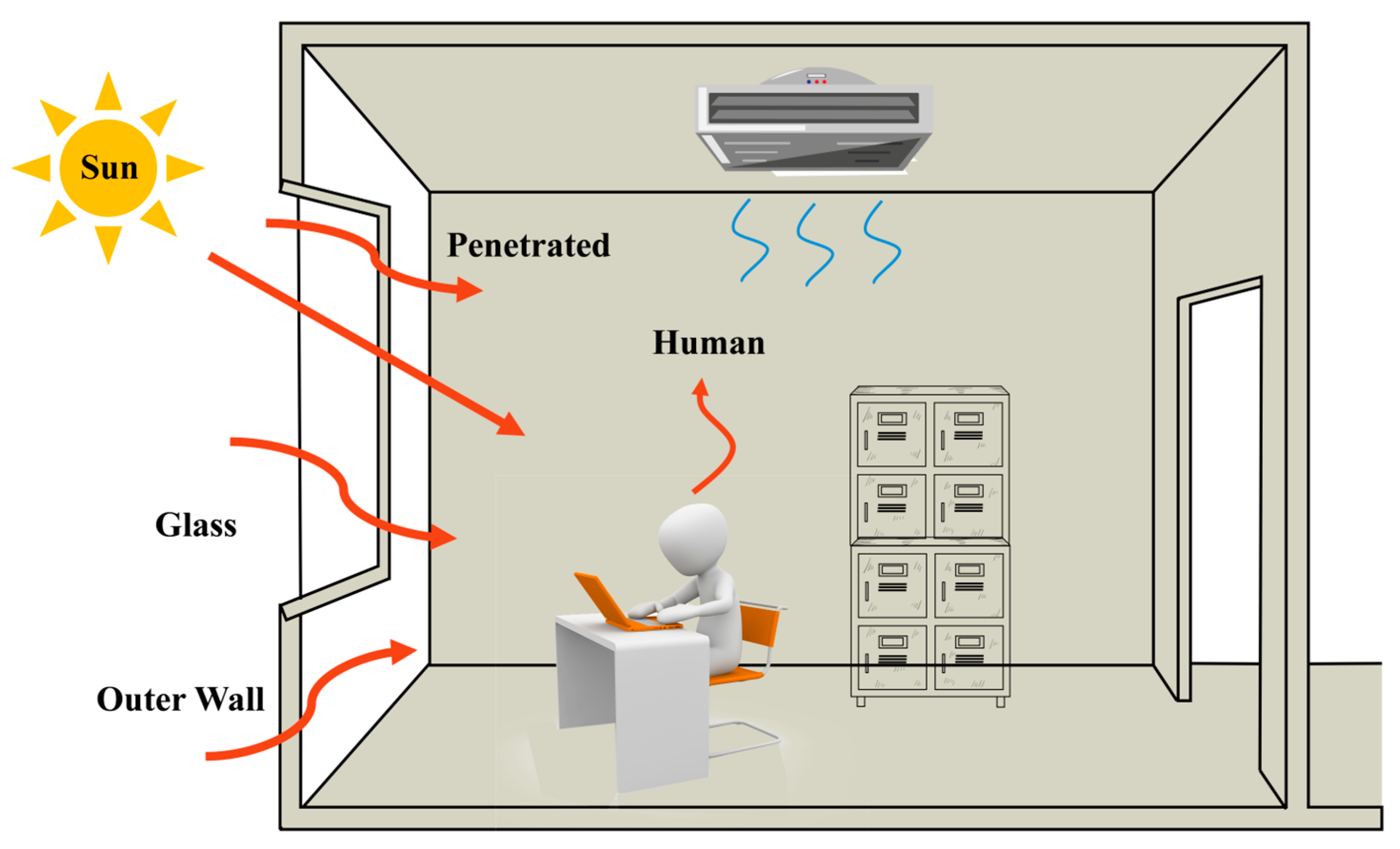
The office building in this study is located in Beijing, China. Therefore, the “Beijing Calculation Base Method” is adopted to calculate the building cooling load. According to the Code for Design of Heating Ventilation and Air Conditioning [36], in addition to using cooling load indicators for necessary estimations during the conceptual or preliminary design stages, a detailed and hourly calculation of the cooling load should be performed for each air-conditioned zone. The total cooling load of the building, ${\mathrm{CL}}_{\mathrm{total}}$ can be calculated as the sum of the summer cooling loads of the air-conditioned zones, as shown in Figure 2, based on the types and properties of the heat gains. The calculation can be expressed by the following formula:

$${\mathrm{CL}}_{\mathrm{total}}{=\mathrm{CL}}_{\mathrm{q}}{+\mathrm{CL}}_{\mathrm{ch}.1}{+\mathrm{CL}}_{\mathrm{ch}.2}{+\mathrm{CL}}_{\mathrm{r}}$$

(4)

where ${\mathrm{CL}}_{\mathrm{q}}$ represents the hourly cooling load formed by the heat transfer through the external walls,${ \mathrm{CL}}_{\mathrm{ch}.1}$ represents the hourly cooling load formed by the heat transfer through the temperature difference of the external windows, ${\mathrm{CL}}_{\mathrm{ch}.2}$ represents the hourly cooling load formed by the solar radiation heat entering the room through the glass windows, and ${\mathrm{CL}}_{\mathrm{r}}$ represents the cooling load caused by the heat dissipation from occupants.

3.2. Establishment of the Chilled Water System Simulation Environment

The cold source system simulation environment is established to accurately simulate and analyze the performance and energy consumption of the central air conditioning system, so as to provide a reliable basis for the research of optimal control algorithms and energy-saving strategies. In this simulation environment, this research considered the equipment parameters, energy consumption calculation method, and operating constraints of the central air conditioning system to ensure that the simulation results match the behavior of the actual system. By establishing such a simulation environment, this research helps us to better understand and optimize the performance of the cold source system, and provides guidance for the energy efficiency improvement of the actual central air conditioning system.

3.2.1. Simulation Environment for the Chilled Water System

This research investigated a widely applied central air conditioning system that utilizes water as the refrigerant and chilled water units as the cooling source. Each type of equipment is represented by a single unit, and their specific parameters are listed in

Table 2. Parameters of the cooling system equipment.

Equipment Type	Parameter	Value
Chiller Unit	Cooling Capacity	120 kW
	Cooling Power	45.3 kW
Cooling Water Pump	Rated Flow Rate	25.5 m3/h
	Rated Power	18.5 kW
	Rated Speed	2900 r/min
	Rated Head	98 m
Chilled Water Pump	Rated Flow Rate	29.2 m3/h
	Rated Power	18.5 kW
	Rated Speed	2900 r/min
	Rated Head	101 m
Cooling Tower	Rated Flow Rate	50 m3/h
	Rated Power	1.5 kW
	Rated Airflow	30,000 m3/h
	Fan Rated Speed	720 r/min

. To maintain a stable indoor design temperature, the cooling capacity of the air conditioning system is set to 1.2 times the building’s cooling load. The main energy-consuming components of the central air conditioning system include chilled water units, chilled water pumps, cooling water pumps, and cooling towers. For example,

$${\mathrm{P}}_{\mathrm{total} }{=\mathrm{P}}_{\mathrm{chiller} }{+ \mathrm{P}}_{\mathrm{pumpe} }{+ \mathrm{P}}_{\mathrm{pumpc} }{+ \mathrm{P}}_{\mathrm{tower} }$$

(5)

where ${\mathrm{P}}_{\mathrm{total} }$ represents the total energy consumption of the central air conditioning system, ${\mathrm{P}}_{\mathrm{chiller} }$ represents the energy consumption of the chilled water units, ${\mathrm{P}}_{\mathrm{pumpe} }$ represents the energy consumption of the chilled water pumps, ${\mathrm{P}}_{\mathrm{pumpc} }$ represents the energy consumption of the cooling water pumps, and ${\mathrm{P}}_{\mathrm{tower} }$ represents the energy consumption of the cooling towers.

The energy consumption of each piece of equipment is represented as follows:

$${\mathrm{P}}_{\mathrm{chiller} \hspace{0.25em}}=\frac{{\mathrm{Q}}_{\mathrm{e}}}{\mathrm{COP}}$$

(6)

$${\mathrm{P}}_{\mathrm{pumpe}} = \frac{{\mathsf{\rho }\mathrm{gV}}_{\mathrm{e}}{\mathrm{H}}_{\mathrm{e}}}{3.6 \times {10}^6\cdot {\mathsf{\eta }}_{\mathrm{e}}}$$

(7)

$${\mathrm{P}}_{\mathrm{pumpc}}=\frac{{\mathsf{\rho }\mathrm{gV}}_{\mathrm{c}}{\mathrm{H}}_{\mathrm{c}}}{3.6 \times {10}^6\cdot {\mathsf{\eta }}_{\mathrm{c}}}$$

(8)

$${\mathrm{P}}_{\mathrm{tower} }={\left(\frac{{\mathrm{f}}_{\mathrm{t}}}{{\mathrm{f}}_0}\right)}^3{\mathrm{P}}_{{\mathrm{tower} }_{-}\mathrm{r}}$$

(9)

where ${\mathrm{Q}}_{\mathrm{e}}$ represents the cooling capacity, $\mathrm{COP}$ denotes the operating efficiency of the chiller unit, ${\mathrm{V}}_{\mathrm{e}}$ is the flow rate of chilled water, ${\mathrm{H}}_{\mathrm{e}}$ represents the head of the chilled water pump, ${\mathsf{\eta }}_{\mathrm{e}}$ denotes the overall efficiency of the chilled water pump, ρ is the density of the fluid, g is the acceleration due to gravity, ${\mathrm{V}}_{\mathrm{c}}$ represents the flow rate of cooling water, ${\mathrm{H}}_{\mathrm{c}}$ denotes the head of the cooling water pump, ${\mathsf{\eta }}_{\mathrm{c}}$ represents the overall efficiency of the cooling water pump, ${\mathrm{f}}_{\mathrm{t}}$ is the operating frequency of the fan, ${\mathrm{f}}_0$ is the rated frequency of the fan, and ${\mathrm{P}}_{{\mathrm{tower} }_{-}\mathrm{r}}$ represents the rated power of the fan.

3.2.2. Constraints

Table 3. Operational parameter constraints for chiller, pump, and cooling tower.

Equipment	Parameter	Constraint
Chiller	Chilled water supply temperature (${\mathrm{T}}_{\mathrm{eo}}$)	7 °C ≤ ${\mathrm{T}}_{\mathrm{eo}}$≤ 12 °C
Pump	Cooling water flow rate (${\mathrm{V}}_{\mathrm{c}}$)	14 m3/h ≤ ${ \mathrm{V}}_{\mathrm{c}}$≤ 29.2 m3/h
	Cooling water pump frequency (${\mathrm{f}}_{\mathrm{c}}$)	23 Hz ≤ ${\mathrm{f}}_{\mathrm{c}}$≤ 50 Hz
	Chilled water flow rate (${\mathrm{V}}_{\mathrm{e}}$)	12 m3/h ≤ ${\mathrm{V}}_{\mathrm{e}}$≤ 25.5 m3/h
	Chilled water pump frequency (${\mathrm{f}}_{\mathrm{e}}$)	23 Hz ≤ ${\mathrm{f}}_{\mathrm{e}}$≤ 50 Hz
Cooling Tower	Cooling water return temperature (${\mathrm{T}}_{\mathrm{ci}}$)	${\mathrm{T}}_{\mathrm{wb}}$≤ ${\mathrm{T}}_{\mathrm{ci}}$≤ 33 °C
	Cooling tower airflow rate (${\mathrm{V}}_{\mathrm{t}}$)	14,000 m3/h ≤ ${\mathrm{V}}_{\mathrm{t}}$≤ 30,000 m3/h
	Cooling tower fan frequency (${\mathrm{f}}_{\mathrm{t}}$)	23 Hz ≤ ${ \mathrm{f}}_{\mathrm{t}}$≤ 50 Hz

summarizes the operational parameter constraints for the chiller, pump, and cooling tower based on the selected equipment’s product manuals and the code for design of heating, ventilation, and air conditioning, considering the strong coupling within the central air conditioning system and the limitations imposed by outdoor weather conditions:

3.3. HVAC System MDP

In a central air conditioning system, the cooling water return temperature of the chiller unit and the cooling tower’s heat dissipation performance are influenced by the cooling water flow rate. Additionally, the cooling water flow rate and the cooling tower airflow affect the heat dissipation performance of the cooling tower. By adjusting the frequency of the cooling water pump, the flow rate of the cooling water can be effectively controlled, and by adjusting the frequency of the cooling tower fan, the airflow of the cooling tower can be changed. The chilled water supply temperature can be controlled by adjusting the set value on the chiller unit, while the chilled water flow rate is related to the frequency of the chilled water pump. Therefore, considering the operating characteristics and interactions of each piece of equipment, this research selected the chilled water supply temperature, chilled water flow rate, cooling water flow rate, and cooling tower airflow as optimization variables for the air conditioning system.

The solution to the reinforcement learning task is based on the MDP. Therefore, this research formulated the optimization problem of the central air conditioning system as an MDP. MDP typically consists of four elements: state space (S), action space (A), state transition probabilities (p), and immediate rewards (r). Here, the state space S represents the intermediate results of energy consumption calculation, action space A represents the set of instructions that the air conditioning controller can execute, state transition probabilities p represent the probabilities of transitioning to the next state after executing different control actions a in states, and immediate rewards r represent the rewards obtained by taking different control actions a in states. This research treated the cooling area of the central air conditioning system as the environment, and the intelligent controller built based on the reinforcement learning algorithm acts as the air conditioning controller. The optimization objective is to reduce the energy consumption required for the operation of the air conditioning system while ensuring indoor comfort.

The MDP parameters of the central air conditioning system are primarily constructed based on the optimization objective. In this study, the energy consumption of the central air conditioning system is taken as the state for reinforcement learning. The chilled water supply temperature, chilled water flow rate, cooling water flow rate, and cooling tower airflow are set as selectable actions. When the reinforcement learning algorithm converges, the output optimal actions correspond to the best control parameters for the cooling system equipment. The state transition probabilities p depend on the true state of the environment after executing control actions, so the algorithm needs to estimate the state transition probabilities p through multiple samples for unbiased estimation. The hourly energy consumption of the central air conditioning system is set as the immediate reward.

4. AFUCB-DQN

When facing large-scale MDPs, the Q-learning algorithm suffers from the problem of explosive memory due to the large number of state–action pairs. In our research, which focuses on the constructed simulation environment of the central air conditioning system, the state space exhibits high-dimensional characteristics. When using the Q-learning algorithm, the high computational complexity and memory storage requirements degrade the algorithm’s performance. To address these issues, this research employed the DQN algorithm, where the approximation capability of neural networks helps improve the stability of the algorithm.

Furthermore, the variance of air conditioning data can lead to environmental variance [37], thereby reducing learning efficiency and causing learning instability and overfitting. To address this problem, this research introduced the advantage function based on the DQN algorithm, aiming to mitigate the impact of air conditioning data variance on environmental variance. This approach enhances learning stability, improves learning efficiency, and prevents overfitting. In the proposed simulation environment of the central air conditioning system, to enhance the robustness of the environment and reduce the gap between the simulation environment and the real environment, this research introduced noise perturbation. However, the presence of noise perturbation can introduce errors in the sampling results. When using the DQN algorithm, traditional ε-greedy exploration cannot avoid the issue of error data, leading to decreased learning efficiency and increased instability. To address this problem, this research adopted the UCB algorithm, which aims to balance the trade-off between exploration and exploitation. It assigns confidence to each action based on its potential value and uncertainty. By calculating and selecting the action with the maximum UCB value based on confidence, this research effectively solved the problem of sampling result errors caused by noise.

4.1. Algorithm Flow

The key components of the AFUCB-DQN algorithm include the neural network, experience replay storage, objective network, and the advantage function. A neural network is used to approximate the Q-value function, which receives a state as input and outputs a corresponding action value. The experience playback storage is used to store the interaction data between the agent and the environment for offline learning. The target network is a fixed copy used to calculate the target Q-value to reduce the target value bias during the learning process. The advantage function is used to calculate the advantage value of each action, which represents its gain relative to the average value, so as to improve the stability of the learning process. In contrast, the traditional DQN algorithm and DDQN algorithm also include neural networks and experience replay storage for learning and storing the Q-value function. However, they do not use advantage functions to account for action value and uncertainty. A key component of the distributed double deep Q-network (D3QN) algorithm also includes the advantage function, which considers the value and uncertainty of each action. However, in terms of algorithm strategy, the D3QN algorithm still adopts the ε-greedy strategy, which is to choose the action with the highest Q-value in the current state [38]. Figure 3 illustrates the pathway process of AFUCB-DQN. The entire process can be divided into the interaction process between the algorithm and the environment and the learning process of the algorithm. In the interaction process between the algorithm and the environment, the energy consumption of the central air conditioning system is first inputted as state $\mathrm{s}$ into the algorithm, which outputs the corresponding action a for state $\mathrm{s}$. When the environment receives the action, it transitions from state $\mathrm{s}$ to state ${\mathrm{s}}_{\mathrm{t}+1}$, and obtains the reward r for action a. At this point, a tuple $\left({\mathrm{s}, \mathrm{a}, \mathrm{r}, \mathrm{s}}_{\mathrm{t}+1}\right)$ is obtained and stored in the experience replay buffer based on the replay memory mechanism. When the experience replay buffer reaches a certain size, the algorithm starts to learn by randomly sampling from the experience replay buffer. First, the current state $\mathrm{s}$ is used as the input of the Evaluate Network, which outputs the actual Q-value $\mathrm{Q}\left(\mathrm{s}, \mathrm{a}, \mathsf{\omega }\right)$. Then, the next state ${\mathrm{s}}_{\mathrm{t}+1}$ is used as the input of the Target Network, which estimates the corresponding Q-value $\underset{\mathrm{a}+1}{\max }\mathrm{Q}\left({\mathrm{s}}_{\mathrm{t}+1}{, \mathrm{a}}_{\mathrm{t}+1}, \mathsf{\omega }\right)$. Next, using $\mathrm{Q}\left(\mathrm{s}, \mathrm{a}, \mathsf{\omega }\right)$, $\underset{\mathrm{a}+1}{\max }\mathrm{Q}\left({\mathrm{s}}_{\mathrm{t}+1}{, \mathrm{a}}_{\mathrm{t}+1}, \mathsf{\omega }\right)$, and the reward r as inputs of the loss function, the mean squared error is obtained. Finally, the algorithm utilizes stochastic gradient descent to update the Evaluate Network and optimize the action selection policy. During this process, the parameters of the Evaluate Network are fully copied to the Target Network after each iteration to ensure the update of the Target Network.

4.2. Advantage Function

The advantage function is a function used in reinforcement learning to evaluate the relative superiority or inferiority of an action compared to other actions. In reinforcement learning, an agent needs to choose the optimal action in a given state to maximize long-term rewards. To achieve this goal, the agent needs to evaluate the potential rewards associated with each possible action in the current state. The advantage function provides an effective way to assess the value of each action, and helps the agent make informed decisions. The advantage function is defined as follows:

$${\mathrm{A}}^{\mathsf{\pi }}\left(\mathrm{s}, \mathrm{a}\right){=\mathrm{Q}}^{\mathsf{\pi }}\left(\mathrm{s}, \mathrm{a}\right) {- \mathrm{V}}^{\mathsf{\pi }}\left(\mathrm{s}\right)$$

(10)

where ${\mathrm{Q}}^{\mathsf{\pi }}(\mathrm{s}, \mathrm{a})$ represents the long-term rewards obtained by choosing action a, and ${\mathrm{V}}^{\mathsf{\pi }}\left(\mathrm{s}\right)$ represents the average long-term rewards obtained in state s. Thus, the advantage function ${\mathrm{A}}^{\mathsf{\pi }}(\mathrm{s}, \mathrm{a})$ represents the additional rewards gained by choosing action a relative to the average action.

The introduction of the advantage function helps to reduce the variance caused by variations in the data of the air conditioning system, as it subtracts a baseline (state value function ${\mathrm{V}}^{\mathsf{\pi }}\left(\mathrm{s}\right)$). By reducing the variance, the advantage function decreases the absolute values of the state value function, thereby improving learning stability. The advantage function decomposes the value function into action value and state value components, reducing their correlation and making the learning process more stable. By using the advantage function, the update processes of the action value and state value can be independent of each other, reducing their mutual interference and improving learning stability. In reinforcement learning, the reward signal is often sparse, which means the agent may need to spend a considerable amount of time exploring the environment to obtain rewards. By computing the advantage function, this research transformed the reward signal into a denser signal, reducing the sparsity of the reward signal and making it easier for the agent to find the optimal policy, thereby improving learning efficiency.

In contrast to the DQN algorithm, the AFUCB-DQN algorithm separates the Q-network value function into two parts: the state value function component $\mathrm{V}\left({\mathrm{s}, \mathsf{\omega }, \mathsf{\omega }}_{\mathrm{V}}\right)$ and the advantage function component $\mathrm{A}\left({\mathrm{s}, \mathrm{a}, \mathsf{\omega }, \mathsf{\omega }}_{\mathrm{A}}\right)$. The state value function component represents the intrinsic value of the static environment itself, dependent only on state s and independent of the specific action a. The advantage function component represents the additional value obtained by choosing an action in a specific state, dependent on both state s and action a. Finally, the two functions are combined to obtain the Q-value corresponding to each action:

$$\mathrm{Q}\left({\mathrm{s}, \mathrm{a}, \mathsf{\omega }, \mathsf{\omega }}_{\mathrm{V}}{, \mathsf{\omega }}_{\mathrm{A}}\right)=\mathrm{V}\left({\mathrm{s}, \mathsf{\omega }, \mathsf{\omega }}_{\mathrm{V}}\right)+\mathrm{A}\left({\mathrm{s}, \mathrm{a}, \mathsf{\omega }, \mathsf{\omega }}_{\mathrm{A}}\right)$$

(11)

where $\mathsf{\omega }$ represents the shared parameters of the neural network, and ${\mathsf{\omega }}_{\mathrm{V}}$ and ${\mathsf{\omega }}_{\mathrm{A}}$ represent the unique neural network parameters for the state value function $\mathrm{V}\left(\mathrm{s}\right)$ and the action advantage function $\mathrm{A}\left(\mathrm{a}\right)$, respectively.

4.3. UCB Algorithm

In the conducted study, the central air conditioning simulation environment that this research established is a complex environment with inherent noise, which can introduce errors in the sampled results. Existing DQNs explore using the ε-greedy strategy, which involves uniform exploration and cannot address the errors caused by exploration. To overcome this issue, this research introduced the UCB algorithm, which aims to balance exploration and exploitation by exploring unknown choices as much as possible and exploiting known rewarding choices. The UCB algorithm assigns a confidence level to each action to balance the trade-off between exploration and exploitation, ensuring that the potential value and uncertainty of actions are considered in each selection. The UCB algorithm selects the next action based on the calculated UCB value. The confidence level comprises the average reward and the confidence interval, where the average reward represents the historical average reward of an action, and the confidence interval represents the uncertainty range of the estimated average reward.

During the learning process, the UCB value for each selection is calculated as follows:

$${\mathrm{UCB}}_{\mathrm{i}}{=\mathrm{X}}_{\mathrm{i}}+\sqrt{\frac{2\mathrm{lnt}}{{\mathrm{N}}_{\mathrm{i}}}}$$

(12)

where ${\mathrm{UCB}}_{\mathrm{i}}$ represents the UCB value of the i-th action, ${\mathrm{X}}_{\mathrm{i}}$ denotes the average reward obtained from selecting the i-th action, ${\mathrm{N}}_{\mathrm{i}}$ is the number of times the i-th action has been chosen, and $\mathrm{t}$ represents the current time step. The UCB algorithm selects the action with the highest UCB value as follows:

$${\mathrm{a}}_{\mathrm{t}}{=\mathrm{argmax}}_{\mathrm{i}=1,\dots ,\mathrm{K}}{\mathrm{UCB}}_{\mathrm{i}}$$

(13)

By replacing the ε-greedy strategy with the UCB algorithm, this research avoided excessive randomness caused by the ε-greedy strategy, and addressed the errors in the sampled results due to the stochasticity of the environment caused by noise. This improvement helps enhance the decision-making performance in the simulation environment.

5. Experiments and Results

This section demonstrates the feasibility and accuracy of the cold source system simulation environment through the description of the experimental setup and the verification of the simulation environment and algorithm, and compares the convergence and energy consumption of different algorithms at different indoor temperatures. These experimental results provide guidance and a basis for the optimization and energy efficiency improvement of the cold source system.

5.1. Experimental Setup

This research simulated an office area located in a public building in Beijing, with a total area of 600 square meter and a ceiling height of 3 meters. The office area accommodated 30 lightly active employees. In the design of the building envelope, this research referred to the Design Standard for Energy Efficiency of Public Buildings [39]. The heat transfer coefficient of the external walls was set to 0.796$\mathrm{W}/\left({\mathrm{m}}^2\cdot °\mathrm{C}\right)$, and the heat transfer coefficient of the windows was set to 3.1$\mathrm{W}/\left({\mathrm{m}}^2\cdot °\mathrm{C}\right)$, with the window area accounting for 80% of the wall area. Considering the working hours of the employees and the simulated environment of the central air conditioning system, this research selected a weather dataset provided by the Xihe Energy Big Data Platform [40]. This dataset included daily weather data from 8:00 to 18:00 between 1 July 2021, and 31 August 2021, including temperature, humidity, solar radiation, and other information.

Regarding the AFUCB-DQN algorithm, the specific design of the deep neural network and hyperparameters are shown in

Table 4. Design of the deep neural network and hyperparameters in the AFUCB-DQN algorithm.

Size of Input	4
No. of hidden layers	2
Size of each hidden layer	[8, 128], [128, 64]
Size of output	4
Activation function	GELU
Optimizer	Adam
Learning rate	10−3
Batch size	64
Discount factor	0.95
Buffer size	128
Delayed policy update U	2

. To enhance the algorithm’s performance, this research selected GELU as the activation function. Compared to other commonly used activation functions such as ReLU and sigmoid, GELU exhibits smoother nonlinear characteristics, which helps improve the algorithm’s performance. Additionally, a sigmoid-like transformation is introduced into the nonlinear transformation of the activation function, allowing the output of the GELU function to span a wider range, thereby accelerating the convergence speed of the model.

5.2. Feasibility Verification of the Validation Environment

To verify the feasibility of the building cooling load simulation environment, this research conducted accuracy validation using 250 sets of building cooling load simulation data. The x-axis of the graph represents the sample number, ranging from 1 to 250, to indicate the sequence and corresponding relationship of each dataset. According to the cooling load standards for office buildings [41], the range of the cooling load is between 128–170 W/m². As shown in Figure 4, the error between the calculated building cooling load from the simulation environment and the cooling load standards is within ±0.8 W/m². This indicates that the simulation environment is suitable for conducting simulation and research on central air conditioning cooling source systems.

To verify the accuracy of the proposed air conditioning system simulation environment, As shown in Figure 5, this research compared the simulated data obtained from our simulation environment with the actual data used in the cooling source system portion of reference [42]. The results show that the power difference between the simulated data and the actual data was within ±7%, indicating that the simulation data can be used for the simulation and research of central air conditioning cooling source systems.

5.3. Algorithm Comparison

According to the Design Code for Heating Ventilation and Air Conditioning of Civil Buildings [43], the thermal comfort level for indoor conditions during summer is classified as Level I, with a temperature range of 24–26 °C and a humidity level of around 50%. To meet the temperature requirements of different individuals, this research compared the performance of different algorithms at indoor temperatures of 24 °C, 25 °C, and 26 °C.

Figure 6 shows the convergence of different algorithms at different room temperatures. It can be observed that, compared with other algorithms, the AFUCB-DQN algorithm exhibits more stable convergence and faster convergence speed under different indoor temperatures, and is able to obtain higher rewards. This can be attributed to two main aspects. First, the AFUCB-DQN algorithm has a better exploration–exploitation balance ability than the DQN algorithm and the DDQN algorithm. The traditional DQN algorithm and DDQN algorithm can only learn the Q-value of taking a specific action in a specific state. When the actions taken in certain states have no significant impact on the final return, the learning time will be wasted. Secondly, the DQN algorithm and the DDQN algorithm use the ε-greedy strategy to explore, but in the face of complex environments with noise, the effectiveness of exploration is low. The AFUCB-DQN algorithm effectively overcomes the shortcomings of the traditional ε-greedy strategy in noisy environments by combining the advantage function and the UCB algorithm. Such improvements enable the algorithm to better cope with complex building cooling load simulation environments, improve the effectiveness of exploration, and achieve more stable and rapid convergence performance. Compared with the D3QN algorithm, although the D3QN algorithm can use the advantage function to consider the value and uncertainty of each action, it still cannot avoid the error data problem when using the ε-greedy strategy for exploration in an environment with noise. Therefore, during the exploration process, the D3QN algorithm may be affected by a certain degree of error data. To sum up, the AFUCB-DQN algorithm, by introducing the consideration of the UCB algorithm and the advantage function, can more effectively solve the problem of error data in the exploration process than the D3QN algorithm, and improve the learning efficiency and stability. It should be noted that the cumulative rewards of the DQN algorithm, DDQN algorithm, and D3QN algorithm are not stable enough, because the existence of the ε-greedy strategy provides a certain probability that the algorithm will explore other non-optimal behaviors, resulting in oscillations.

Figure 7 illustrates the energy consumption of different algorithms for each sample at different indoor temperatures. It can be observed that the AFUCB-DQN algorithm consistently achieves significantly lower energy consumption compared to the DQN algorithm, DDQN algorithm, and D3QN algorithm. Additionally, the AFUCB-DQN algorithm demonstrates stable energy-saving performance. To provide a more intuitive representation of the energy-saving effect, Figure 8 presents the average hourly energy consumption of the DQN algorithm, DDQN algorithm, and D3QN algorithm, and of the AFUCB-DQN algorithm, in the central air conditioning system at indoor temperatures of 24 °C, 25 °C, and 26 °C. The figure also indicates the percentage reduction in energy consumption achieved by each algorithm compared to the original energy consumption. Therefore, while meeting the thermal comfort requirements of different individuals during the summer, the AFUCB-DQN algorithm exhibits significant energy-saving benefits compared to the DQN algorithm, DDQN algorithm, and D3QN algorithm.

6. Conclusions and Future Work

This study proposes an innovative method that combines the building cooling load simulation environment, the cooling source system, and deep reinforcement learning to optimize the control strategy of the central air conditioning system, and proposes the cooling source system control based on the AFUCB-DQ algorithm optimization method. This method improves the stability of the learning process by using the advantage function, and obtains a better exploration–utilization balance ability by introducing the UCB algorithm, avoiding the error data problem that may occur during the exploration process. By comprehensively considering various factors of building cooling load and introducing noise interference, this study constructs an accurate and robust central air conditioning system simulation environment, which can dynamically adjust the operating parameters of the cooling source system according to the actual cooling load demand. After training and comparative analysis of the AFUCB-DQN algorithm, this research found that under the premise of indoor thermal comfort requirements in summer, compared with the DQN algorithm, DDQN algorithm, and D3QN algorithm, the algorithm shows more stable convergence, faster convergence speed, and higher rewards, resulting in energy optimization and significant improvements in energy savings. The operating parameters of the cold source system obtained by the proposed method can provide effective guidance for the operation of the actual central air conditioning system. The main focus of this research is the optimization of energy consumption and energy saving effect under the requirement of indoor thermal comfort in summer. However, for room use requirements in other seasons or different working conditions, the applicability and effect of this method still need further verification and exploration. Future research should consider meeting the room use requirements under different working conditions, and explore methods, such as multi-connected air conditioning systems and multi-agent reinforcement learning, to solve related problems, and extend the scope of optimization control to energy-saving optimization throughout the year.

The central air conditioning system control optimization method proposed in this study not only realizes the improvement in energy saving effect and the guarantee of indoor thermal comfort, but also provides guidance and reference for practical application.

References

- Perez-Lombard, L.; Ortiz, J.; Maestre, I.R. The Map of Energy Flow in HVAC Systems. Appl. Energy 2011, 88, 5020–5031. [Google Scholar] [CrossRef]
- Tang, R.; Wang, S.; Sun, S. Impacts of Technology-Guided Occupant Behavior on Air-Conditioning System Control and Building Energy Use. Build. Simul. 2021, 14, 209–217. [Google Scholar] [CrossRef]
- Chen, J.; Sun, Y. A New Multiplexed Optimization with Enhanced Performance for Complex Air Conditioning Systems. Energy Build. 2017, 156, 85–95. [Google Scholar] [CrossRef]
- Gholamzadehmir, M.; Del Pero, C.; Buffa, S.; Fedrizzi, R.; Aste, N. Adaptive-Predictive Control Strategy for HVAC Systems in Smart Buildings—A Review. Sustain. Cities Soc. 2020, 63, 102480. [Google Scholar] [CrossRef]
- Lu, Y.; Khan, Z.A.; Alvarez-Alvarado, M.S.; Zhang, Y.; Huang, Z.; Imran, M. A Critical Review of Sustainable Energy Policies for the Promotion of Renewable Energy Sources. Sustainability 2020, 12, 5078. [Google Scholar] [CrossRef]
- Mariano-Hernandez, D.; Hernandez-Callejo, L.; Zorita-Lamadrid, A.; Duque-Perez, O.; Santos Garcia, F. A Review of Strategies for Building Energy Management System: Model Predictive Control, Demand Side Management, Optimization, and Fault Detect & Diagnosis. J. Build. Eng. 2021, 33, 101692. [Google Scholar]
- Gao, J.; Yang, X.; Zhang, S.; Tu, R.; Ma, H. Event-Triggered Distributed Model Predictive Control Scheme for Temperature Regulation in Multi-Zone Air Conditioning Systems with Improved Indoor Thermal Preference Indicator. Int. J. Adapt. Control Signal Process. 2023, 37, 1389–1409. [Google Scholar] [CrossRef]
- Salins, S.S.; Kumar, S.S.; Thommana, A.J.J.; Vincent, V.C.; Tejero-Gonzalez, A.; Kumar, S. Performance Characterization of an Adaptive-Controlled Air Handling Unit to Achieve Thermal Comfort in Dubai Climate. Energy 2023, 273, 127186. [Google Scholar] [CrossRef]
- Aruta, G.; Ascione, F.; Bianco, N.; Mauro, G.M.; Vanoli, G.P. Optimizing Heating Operation via GA- and ANN-Based Model Predictive Control: Concept for a Real Nearly-Zero Energy Building. Energy Build. 2023, 292, 113139. [Google Scholar] [CrossRef]
- Yang, S.; Yu, J.; Gao, Z.; Zhao, A. Energy-Saving Optimization of Air-Conditioning Water System Based on Data-Driven and Improved Parallel Artificial Immune System Algorithm. Energy Convers. Manag. 2023, 283, 116902. [Google Scholar] [CrossRef]
- Sun, F.; Yu, J.; Zhao, A.; Zhou, M. Optimizing Multi-Chiller Dispatch in HVAC System Using Equilibrium Optimization Algorithm. Energy Rep. 2021, 7, 5997–6013. [Google Scholar] [CrossRef]
- Tang, R.; Wang, S. Model Predictive Control for Thermal Energy Storage and Thermal Comfort Optimization of Building Demand Response in Smart Grids. Appl. Energy 2019, 242, 873–882. [Google Scholar] [CrossRef]
- Utama, C.; Troitzsch, S.; Thakur, J. Demand-Side Flexibility and Demand-Side Bidding for Flexible Loads in Air-Conditioned Buildings. Appl. Energy 2021, 285, 116418. [Google Scholar] [CrossRef]
- Sutton, R.; Barto, A. Reinforcement Learning; MIT Press: Cambridge, MA, USA, 1998. [Google Scholar]
- Goodfellow, I.; Bengio, Y.; Courville, A. Deep Learning; MIT Press: Cambridge, MA, USA, 2016. [Google Scholar]
- Li, W.; Todorov, E. Iterative Linear Quadratic Regulator Design for Nonlinear Biological Movement Systems. In Proceedings of the International Conference on Informatics in Control, Automation and Robotics, Setubal, Portugal, 28 August 2004. [Google Scholar]
- Zhao, H.; Zhao, J.; Shu, T.; Pan, Z. Hybrid-Model-Based Deep Reinforcement Learning for Heating, Ventilation, and Air-Conditioning Control. Front. Energy Res. 2021, 8, 610518. [Google Scholar] [CrossRef]
- Chen, L.; Meng, F.; Zhang, Y. MBRL-MC: An HVAC Control Approach via Combining Model-Based Deep Reinforcement Learning and Model Predictive Control. IEEE Internet Things J. 2022, 9, 19160–19173. [Google Scholar] [CrossRef]
- Wang, Z.; Hong, T. Reinforcement Learning for Building Controls: The Opportunities and Challenges. Appl. Energy 2020, 269, 115036. [Google Scholar] [CrossRef]
- Biemann, M.; Scheller, F.; Liu, X.; Huang, L. Experimental Evaluation of Model-Free Reinforcement Learning Algorithms for Continuous HVAC Control. Appl. Energy 2021, 298, 117164. [Google Scholar] [CrossRef]
- Heo, S.; Nam, K.; Loy-Benitez, J.; Li, Q.; Lee, S.; Yoo, C. A Deep Reinforcement Learning-Based Autonomous Ventilation Control System for Smart Indoor Air Quality Management in a Subway Station. Energy Build. 2019, 202, 109440. [Google Scholar] [CrossRef]
- Yuan, X.; Pan, Y.; Yang, J.; Wang, W.; Huang, Z. Study on the Application of Reinforcement Learning in the Operation Optimization of HVAC System. Build. Simul. 2021, 14, 75–87. [Google Scholar] [CrossRef]
- Wei, T.; Wang, Y.; Zhu, Q. Deep Reinforcement Learning for Building HVAC Control. In Proceedings of the 54th Annual Design Automation Conference 2017, Austin, TX, USA, 18 June 2017. [Google Scholar]
- Deng, X.; Zhang, Y.; Qi, H. Towards Optimal HVAC Control in Non-Stationary Building Environments Combining Active Change Detection and Deep Reinforcement Learning. Build. Environ. 2022, 211, 108680. [Google Scholar] [CrossRef]
- Lei, Y.; Zhan, S.; Ono, E.; Peng, Y.; Zhang, Z.; Hasama, T.; Chong, A. A Practical Deep Reinforcement Learning Framework for Multivariate Occupant-Centric Control in Buildings. Appl. Energy 2022, 324, 119742. [Google Scholar] [CrossRef]
- Marantos, C.; Lamprakos, C.P.; Tsoutsouras, V.; Siozios, K.; Soudris, D. Towards Plug&Play Smart Thermostats Inspired by Reinforcement Learning. In Proceedings of the Workshop on INTelligent Embedded Systems Architectures and Applications, Turin, Italy, 4 October 2018. [Google Scholar]
- Zhang, Z.; Chong, A.; Pan, Y.; Zhang, C.; Lu, S.; Lam, K.P. A Deep Reinforcement Learning Approach to Using Whole Building Energy Model for HVAC Optimal Control. In Proceedings of the 2018 Building Performance Analysis Conference and SimBuild, Chicago, IL, USA, 26–28 September 2018. [Google Scholar]
- Wang, Y.; Velswamy, K.; Huang, B. A Long-Short Term Memory Recurrent Neural Network Based Reinforcement Learning Controller for Office Heating Ventilation and Air Conditioning Systems. Processes 2017, 5, 46. [Google Scholar] [CrossRef] [Green Version]
- Ding, Z.-K.; Fu, Q.-M.; Chen, J.-P.; Wu, H.-J.; Lu, Y.; Hu, F.-Y. Energy-Efficient Control of Thermal Comfort in Multi-Zone Residential HVAC via Reinforcement Learning. Connect. Sci. 2022, 34, 2364–2394. [Google Scholar] [CrossRef]
- Zhang, Z.; Chong, A.; Pan, Y.; Zhang, C.; Lam, K.P. Whole Building Energy Model for HVAC Optimal Control: A Practical Framework Based on Deep Reinforcement Learning. Energy Build. 2019, 199, 472–490. [Google Scholar] [CrossRef]
- Gao, G.; Li, J.; Wen, Y. Deep Comfort: Energy-Efficient Thermal Comfort Control in Buildings Via Reinforcement Learning. IEEE Internet Things J. 2020, 7, 8472–8484. [Google Scholar] [CrossRef]
- Li, Z.; Sun, Z.; Meng, Q.; Wang, Y.; Li, Y. Reinforcement Learning of Room Temperature Set-Point of Thermal Storage Air-Conditioning System with Demand Response. Energy Build. 2022, 259, 111903. [Google Scholar] [CrossRef]
- Watkins, C.; Dayan, P. Q-Learning. Mach. Learn. 1992, 8, 279–292. [Google Scholar] [CrossRef]
- Duan, Y.; Chen, X.; Houthooft, R.; Schulman, J.; Abbeel, P. Benchmarking Deep Reinforcement Learning for Continuous Control. In Proceedings of the International Conference on Machine Learning, New York, NY, USA, 20–22 June 2016. [Google Scholar]
- Mnih, V.; Kavukcuoglu, K.; Silver, D.; Graves, A.; Antonoglou, I.; Wierstra, D.; Riedmiller, M. Playing Atari with Deep Reinforcement Learning. arXiv 2013, arXiv:1312.5602. [Google Scholar]
- GB 50019-2003; Code for Design of Heating Ventilatian and Air Gonditioning. China Planning Press: Beijing, China, 2003.
- Sun, L.; Wu, J.; Jia, H.; Liu, X. Research on Fault Detection Method for Heat Pump Air Conditioning System under Cold Weather. Chin. J. Chem. Eng. 2017, 25, 1812–1819. [Google Scholar] [CrossRef]
- Li, Y.; Wang, Z.; Xu, W.; Gao, W.; Xu, Y.; Xiao, F. Modeling and Energy Dynamic Control for a ZEH via Hybrid Model-Based Deep Reinforcement Learning. Energy 2023, 277, 127627. [Google Scholar] [CrossRef]
- GB 50189-2015; Design Standard for Energy Efficiency of Public Buildings. China Architecture and Building Press: Beijing, China, 2015.
- National Aeronautics and Space Administration. Data Are Based on Historical Reanalysis Datasets from the European Centre for Medium-Range Weather Forecasts (ECMWF). Available online: https://www.xihe-energy.com (accessed on 24 May 2022).
- Lu, Y. Practical Design Manual for Heating and Air Conditioning, 2nd ed.; China Architecture and Building Press: Beijing, China, 2008. [Google Scholar]
- Huang, Y. Study of Operation Optimization for Cold Source System of Central Air-Conditioning Based on TRNSYS. Ph.D. Thesis, South China University of Technology, Chengdu, China, 2015. [Google Scholar]
- GB 50736-2012; Design Code for Heating Ventilation and Air Conditioning of Civil Buildings. China Architecture and Building Press: Beijing, China, 2012.
Figure 1.
Reinforcement learning process.
Figure 2.
Types of heat comprising the building cooling load.
Figure 3.
Schematic diagram of the AFUCB-DQN algorithm model.
Figure 4.
Validation of building cooling load simulation environment data.
Figure 5.
Validation of the cooling source system simulation environment.
Figure 6.
Convergence comparison of different algorithms at different indoor temperatures. (a) Indoor temperature of 24 °C, (b) indoor temperature of 25 °C, and (c) indoor temperature of 26 °C.
Figure 7.
Energy consumption comparison of different algorithms for each sample at different indoor temperatures. (a) Indoor temperature of 24 °C, (b) indoor temperature of 25 °C, and (c) indoor temperature of 26 °C.
Figure 8.
Comparison of the hourly average energy consumption of different algorithms and the original energy consumption at different indoor temperatures.