Model Calibration of Stochastic Process and Computer Experiment for MVO Analysis of Multi-Low-Frequency Electromagnetic Data

Abstract

An electromagnetic (EM) technique is employed in seabed logging (SBL) to detect offshore hydrocarbon-saturated reservoirs. In risk analysis for hydrocarbon exploration, computer simulation for subsurface modelling is a crucial task. It can be expensive and time-consuming due to its complicated mathematical equations, and only a few realizations of input-output pairs can be generated after a very lengthy computational time. Understanding the unknown functions without any uncertainty measurement could be very challenging as well. We proposed model calibration between a stochastic process and computer experiment for magnitude versus offset (MVO) analysis. Two-dimensional (2D) Gaussian process (GP) models were developed for low-frequencies of 0.0625–0.5 Hz at different hydrocarbon depths to estimate EM responses at untried observations with less time consumption. The calculated error measurements revealed that the estimates were well-matched with the computer simulation technology (CST) outputs. Then, GP was fitted in the MVO plots to provide uncertainty quantification. Based on the confidence intervals, hydrocarbons were difficult to determine especially when their depth was 3000 m from the seabed. The normalized magnitudes for other frequencies also agreed with the resulting predictive variance. Thus, the model resolution for EM data decreases as the hydrocarbon depth increases even though multi-low frequencies were exercised in the SBL application.

1. Introduction

The electromagnetic (EM) imaging technique for geophysical applications is categorized as a geo-electrical method family which can be grouped into two types, active and passive [1]. The marine controlled-source electromagnetic (CSEM) surveying technique is classified as an active method due to the character of its EM source. In offshore hydrocarbon exploration, marine CSEM is also known as seabed logging (SBL). SBL is an application of the EM technique for marine hydrocarbon prospecting in the deep offshore environment. This application has become a promising tool to detect, characterize, and map offshore hydrocarbon-filled reservoirs. Since the early 2000s, it has gained wide acceptance in the oil and gas industry. Due to rapid development of the EM technique, it is now a well-established surveying technique for offshore hydrocarbon exploration based on the technology of horizontal source and receiver sensors (see [2,3,4] for references). Generally, this application detects the contrasts of the electrical resistivity, exploiting the fact that a hydrocarbon-filled reservoir has a higher resistivity than its surroundings. The traditional surveying technique (i.e., seismic surveying) uses acoustic waves to acquire structural information about the lithology of the subsurface beneath the seabed, while SBL applications can provide information of pre-drilling discrimination whether the potential reservoir (i.e., prospect) contains hydrocarbon or not.

SBL application utilizes a powerful electric dipole to continuously transmit a periodic low-frequency EM signal through seawater and the subsurface in all directions. The frequency exercised in the SBL application is usually between 0.01 Hz and 10 Hz. Typically, the electric dipole transmitter is towed at an elevation of 30–50 m above the seabed surface. Due to the behavior of the EM waves, the geometry characteristics of the highly-resistive layer (e.g., hydrocarbon) under the seabed can be identified. The electric and magnetic receivers are positioned on the seabed to record the transmitted EM signal. These receivers can record different types of waves, such as direct waves, air waves, and the reflected and refracted wave, from the subsurface interaction. Detection of the reflected and refracted waves from the highly-resistive body beneath the seabed is the basis and main contribution to the SBL data interpretation. According to [2], this wave is known as a guided wave. When this wave enters a hydrocarbon-saturated reservoir, it flows along the resistive layer before reaching the seabed receivers. Thus, the receivers contain information of the geological structure underneath the seabed.

In the application of geophysics, numerical modelling is the most crucial part, especially when it comes to the context of subsurface/reservoir modelling. The finite element (FE) method is one of the most famous techniques exercised in EM problems due to its capability of modelling such a complex geological structure in the deep offshore environment. This computational method exercises unstructured grids so that it can realistically replicate the complex structure [5]. The robustness of the FE method is undoubted; however, this technique requires very high computational time to obtain linear solutions. Researchers in [6,7] mentioned that the most time-consuming part in the FE algorithms is solving the linear equations system, not to mention for inversion scheme since it needs multiple EM forward solutions [7]. Computer simulations from complex computer models usually are either very costly or time-consuming or both. Consequently, only very few realizations of input and output combinations of the computer simulation outputs are available after a very lengthy computational time. Furthermore, reservoir models are constructed based on a very large amount of noisy data through computer simulations. Understanding the unknown functions from multiple possible outputs of reservoir models is the other crucial part, especially to quantify the uncertainties of the data. When the depth of the resistive body gets deeper, the EM response become very difficult to distinguish with a reference response (a response from a non-hydrocarbon region). Due to these constraints, many researchers have looked forward to reducing the computational time in the data interpretation. Researchers in [5] mentioned that if there is a possibility to de-risk a known prospect, any additional information that is able to be collected will be beneficial to the exploration.

Thus, in order to seek the most favorable balance between modelling accuracy associated with uncertainty quantification in the forward modelling and computational cost involved in the computer simulations, we propose a methodology of model calibration between a well-known stochastic process, namely Gaussian process (GP) regression, and computer experiments using computer simulation technology (CST) software in the magnitude versus offset (MVO) analysis. Note that the SBL data interpretation approach is commonly based on analyzing the normalized magnitude versus offset (MVO) plot [8]. This is based on the assumption that if the reference EM magnitude can be obtained from a region where the absence of the hydrocarbon-filled reservoir has been confirmed, the normalized MVO could determine the presence of the resistive body. This happens because the attenuation of the electric field (E-field) when the hydrocarbon reservoir is present is lower with distance compared to the E-field attenuation at the reference region. In the literature, the GP methodology was successfully employed to estimate the EM responses in the EM forward modelling (refer to [9,10] for details), however, applying model calibration of the probabilistic technique and the simulation modelling from the computer experiment on MVO analysis of multi-low-frequency EM data is a novel methodology in the EM application.

Basically, this paper preferentially highlights the MVO analysis of one-dimensional (1D) SBL data in the risk analysis by calibrating models developed by the stochastic process and the CST outputs. Although the current numerical techniques are very powerful and capable of providing good representation of the marine CSEM models, this attempt is very helpful in certain ways especially when the data are insufficient. Rather than acquiring the SBL data using computer simulation software for all possible parameters (e.g., offset, depth, frequency etc.) which consequently requires high computational time due to the complexity of its deterministic models, stochastic process of multivariate GP regression methodology is more efficient where it is capable of providing reliable information of the EM responses with uncertainty quantification and has low time consumption. Hence, it could reduce the data-processing time of acquiring EM responses in the SBL simulation. The main idea of this research work is that two-dimensional (2D) GP regression is used to estimate and model the EM profile at untried low transmission frequencies (0.0625–0.5 Hz) by utilizing the tried CST computer outputs as the prior information. Then, the GP is fitted in the MVO plots to quantify the uncertainty of the presence of the hydrocarbon in terms of variance in order to understand the behavior of the EM responses towards multi-low-frequency EM signals (especially at a hydrocarbon depth of 3000 m) in hydrocarbon detection. Hence, the most suitable transmission frequency that can give the best model resolution for hydrocarbon detection in various depths could be pre-identified before exploration is done. This could be implemented in scanning or risk analysis involved in the SBL application to explore the prospects. The section below briefly discusses the literature on the GP and the CST software.

2. Model Calibration

Computer experiments are not new among scientists, engineers, and researchers around the world. For decades, computer experiments have successfully been used in the application of science, technology, and engineering. Nowadays, scientists prefer to utilize computer simulations that involve mathematical models rather than doing case study observations or conducting physical experiments. The main reason for using computer simulations is that they can be implemented in any circumstances, including experiments that are impossible to be done physically in a real situation. Many factors can be considered as major contributions to the increase of usage of the computer simulations, such as long-term cost effect, safety issues, low time taken for the data acquisition, etc. As early as the 1980s, computer codes that represented a model of fluid-dynamics for flames had been described by researchers in [11]. They mentioned that the computer code was able to solve a complex set of partial differential equations (PDEs) where the input variables consisted of parameters for five different chemical reactions corresponding to the velocity of the flames. For additional literature, [12] described several other research works in different applications that utilized computer experiments to simulate physical experiments/phenomena for designing and predictive purposes.

Computer experiments are run by means of computer code and highly-developed theories of mathematics, physics, and engineering. Researchers in [12] and subsequent works modeled the computer output, $Y\left(x\right)$, which depended on the input parameter, $x$, as the sum of regression terms, ${\beta }_i$, and stochastic component, $S\left(x\right)$. The regression part depends on the known functions, $f_i\left(x\right)$, where $i=1,2,\dots ,k$. Thus, the computer output model is defined by Equation (1):

$$Y\left(x\right)={{\displaystyle \sum }}_{i=1}^k{\beta }_i{f}_i\left(x\right)+S\left(x\right),$$

(1)

where $S\left(x\right)$ represents a random stochastic process with zero mean and covariance,

$$J\left(x,x^{\prime }\right)={\sigma }^{2}C\left(x,x^{\prime }\right).$$

(2)

From Equation (2),$C\left(x,x^{\prime }\right)$ is the correlation function between $S\left(x\right)$ and $S\left(x^{\prime }\right)$. The idea behind this concept is although $Y\left(x\right)$ is a deterministic function, the complex departures of $Y\left(x\right)$ from the regression part may bear a resemblance to the realization of an appropriately-chosen stochastic process, $S\left(x\right)$. There are a lot of choices of stochastic process, but the Gaussian process (GP) is the most famous choice of $S\left(x\right)$ as the distribution of each $S\left(x\right)$ is treated and assumed as a Gaussian (normal) distribution with a mean function and a covariance function. Researchers in [13] mentioned that GP can become a surrogate model for any intricate mathematical models that require lengthy computational time to solve. The features of being flexible to represent the computer output, $Y\left(x\right)$, and easy to obtain analytical formulas make the GP methodology a very popular stochastic process.

Based on the literature, there are many studies related to different aspects of computer experiments and statistical methodology. Researchers in [12] discussed the prediction of untried points based on kriging equations defined from the GP methodology. Researchers in [14] also thoroughly discussed predictive and issues obtained in designing equations involved in the computer experiments for choosing correlation function. More recent studies on computer models have focused on the model calibration, measurement of uncertainty, and model validation for multivariate and functional outputs. Model calibration is a process of choosing appropriate model parameters of computer code, so that the real-field data can be well-approximated by the computer model. The main key to this process is the consideration of selecting a good correlation function that can measure the discrepancy between the computer response and the real-field data and accurately mimic actual values (examples can be found in [15]). Researchers in [16] also described model calibration for high-dimensional multivariate output. Next is model validation: Model validation is a process of assessing whether data obtained from the computer model approximate the real-field data with an acceptable accuracy or not. As the examples from [17,18,19] explained validation of computer models from a frequentist viewpoint, [20] discussed the methodology of Bayesian model validation for computer outputs. The details on the GP and the CST software are discussed in Section 2.1 and Section 2.2

2.1. Gaussian Process (GP)

GP is a well-known technique that has been applied in many applications. This technique has been adopted in scientific and engineering fields, comprising of machine learning, geo-statistics, electronics, etc. This stochastic technique became very popular due to its capability of being flexible, probabilistic and non-parametric. GP has convenient properties for modelling in statistics applications and machine learning. According to [21], GP regression has demonstrated outstanding performance in plenty of studies. It is a simple and elegant approach where it works well in modelling non-linear problems for probabilistic networks [22]. Since GP is a probabilistic kernel machine, it can provide predictive mean and variance through Bayesian inference. Researchers in [23] mentioned that GP has no restriction on the composition of the mean function and the covariance function. The generic framework provided by the GP can be exercised in many problems/applications especially in regression, interpolation, and prediction where a deterministic function is not able to be obtained [24].

Here, we provide the literature of GP in applications other than computer experiments. Researchers in [25] investigated the ability of the GP regression to predict load-bearing piles capacity by comparing performances of the GP, the support vector machine (SVM) approach, and empirical relations. They found that GP regression worked very well in predicting the piles capacity as compared to the SVM and empirical relations. Researchers in [26] asserted that low cost and low complex proximity reports for received-signal-strength (RSS) threshold were obtained when using GP. In the electronic field, [27] utilized GP to describe the uncertainty of estimation in the state of health (SOH) of lithium-ion batteries. Next, researchers in [28] stated that GP was able to reduce the complexity in the computer vision with a better quality of reconstruction. Additionally, this probabilistic approach has also been used in chemical applications. For example, [29] used GP regression to predict particle diameters of nickel pellets. The findings revealed that analysis using GP and a counting rule was capable of yielding good performance with a small mean absolute percentage error (MAPE). For geophysics problems, researchers in [30] claimed that GP regression was an efficient approach to obtain reliable information of porosity and permeability in well analysis.

2.2. Computer Simulation Technology (CST) Software

CST EM STUDIO (CST EMS) is a commercial EM software/tool (CST Studio Suite Research Base Pack (CST 2019), Dassault Systèmes, Vélizy-Villacoublay, France) that provides powerful computational solutions to simulate and design low-frequency applications. As described in [31], this low-frequency solver is capable of discretizing Maxwell’s equations using the finite integration method (FIM). In EM problems, Maxwell’s equations are utilized to predict the propagation phenomenon of low-frequency EM signal (i.e., strength of E-field) travelling through different mediums in order to probe contrast of resistivity. The FIM solves the equations in a finite calculation domain which is in grid cell of hexahedral or tetrahedral mesh element. Maxwell’s equations involved in the software are defined by Equations (3)–(6):

$${\int }_{\partial A}\overrightarrow{E}.\overrightarrow{ds}=-\frac{\partial }{\partial t}\int {\int }_A\overrightarrow{B}.\overrightarrow{dA},$$

(3)

$${\int }_{\partial A}\overrightarrow{H}.\overrightarrow{d}s=\int {\int }_A\left[\frac{\partial \overrightarrow{D}}{\partial t}+\overrightarrow{j}\right].\overrightarrow{dA},$$

(4)

$$\int {\int }_{\partial V}\overrightarrow{B}.\overrightarrow{dA}=0,$$

(5)

$${\iint }_{\partial V}\overrightarrow{D}.\overrightarrow{dA}=Q.$$

(6)

CST software has been used in many applications especially in EM problems due to its user-friendliness and flexibility. Researchers in [32] stated that CST software can be used to replicate SBL applications to acquire synthetic SBL data/responses. Researchers in [33] also suggested CST software as the synthetic SBL data acquisition tool. Studies related to the usage of the CST software in EM applications can be found in [34,35,36,37,38,39]. Details of the CST software can be found in [40].

3. Methodology

This section consists of three subsections, which include the SBL modelling using CST software, developing the forward GP models for every low transmission frequency and hydrocarbon depth, and model validation between computer simulation outputs and the estimates by using different statistical forecast error measurements.

3.1. Seabed Logging (SBL) Modelling

In this research work, typical synthetic SBL models for hydrocarbon exploration were replicated using CST software. SBL models with the presence of hydrocarbon are called target models, while the SBL model with no hydrocarbon layer is called a reference model. As mentioned earlier, we focused on the application of multi-low-frequency EM signals (from 0.0625 to 0.5 Hz with an increment of 0.0625 Hz each) to study the effect of these frequencies towards the magnitude versus offset (MVO) plots at far source-receiver separation distances. For the target model, a 200 m-thick resistive body (hydrocarbon layer) was located at certain depths underneath the seabed. We considered three different depths of hydrocarbon, which were 1000 m, 2000 m, and 3000 m from the seabed surface (seafloor) while, for the reference model, no hydrocarbon layer was embedded in the sediment layer. Note that the depth of the hydrocarbon layer and the transmission frequency were the computer model parameters. For every different set of these two parameters, a dataset of 1D SBL or EM responses was generated through the simulation software. Figure 1 shows the basic illustration of the SBL models at the xz cross-section used in this research work.

CST software modeled and simulated the SBL with defined parameters. The length, width, and height of the developed SBL models (target and reference models) were 20,000 m, 20,000 m, and 5000 m, respectively. Target models consisted of four layers, and every layer has its own unique thickness (air = 300 m; seawater = 1000 m; hydrocarbon = 200 m; sediment = 3500 m). The hydrocarbon layer was embedded in the sediment layer. The overburden layer is the sediment above the hydrocarbon layer. The thickness of the overburden layer represents the depth of the hydrocarbon medium. While for the reference model, thicknesses of air and seawater layers remained so parameterized in the target model, the sediment layer was fixed to have a thickness of 3700 m. We considered both the hydrocarbon and sediment layers as isotropic media. Each of the layers were parameterized with reliable electrical conductivity (reciprocal of electrical resistivity). We tabulated the properties in

Table 1. Electrical conductivity values used in the SBL modelling were taken from [36]. Note that electrical resistivity is the inverse of electrical conductivity.

Layer	Electrical Conductivity (S/m)
Air	1.00 × 10−11
Seawater	1.63
Sediment (overburden & under burden)	1.00
Hydrocarbon (HC)	2.00 × 10−3

.

A 270 m-long horizontal electrical dipole (HED) transmitter was used as the source of the EM signal. This transmitter was positioned in the seawater at the center of the SBL model (x = 10,000 m; y = 10,000 m) in the orientation of x-direction and at an elevation of 30 m above the seabed surface. The HED source was kept stationary (static source-receiver separation) and the current strength used in this research work was 1250 A. Inline receivers were located along the x-direction (0–20,000 m) at y = 10,000 m on the seabed. Then, data acquired from the CST software were processed using a GP regression methodology. The details were described in the subsection below.

3.2. Stochastic Process–GP Regression

Theoretically, GP is a random function $f$ at which any finite number of the function is normally distributed (Gaussian distribution). This stochastic process is fully defined by a mean function, $m\left(x\right)$, and a covariance function, $k\left(x,x^{\prime }\right)$ which are evaluated in terms of vector and matrix, respectively. By simplicity, the GP regression usually employs zero-mean function. Assuming the training set (from the CST computer output), $y$, of $n$ number of parameters which represented the magnitude of E-field (EM response) having input parameter, $x$, where $x=\left(p,q\right)$ for the two-dimensional (2D) model and $x=p$ for the one-dimensional (1D) regression model. In this paper, $p$ denotes the source-receiver separation distance (offset) and $q$ denotes the transmission frequency at every tested depth of hydrocarbon. Thus, the input, $x\in {ℝ}^{n=2}$ (for 2D) and $x\in {ℝ}^{n=1}$ (for 1D), and the corresponding output, $y\in ℝ$. The GP model on $f$ with a zero-mean function, $m\left(x\right)=0$, was therefore defined in Equation (7):

$$f\left(x\right)~GP\left(0,k\left(x,x^{\prime }\right)\right),$$

(7)

where $GP$ was the Gaussian process and $k\left(x,x^{\prime }\right)$ was the covariance function. Generally, $m\left(x\right)$ indicates an expectation value of the function $f$, while $k\left(x,x^{\prime }\right)$ measures the correlation between input data.

We used a very famous covariance function, namely, squared exponential (SE), to govern the smoothness of the GP realizations which was dictated by the CST computer output. For the SE covariance function, as the distance between the input pairs of the offset and frequency of the EM wave increases, the covariance between these input pairs is exponentially decreased. The SE covariance function is represented by Equation (8):

$$k\left(x,x^{\prime }\right)={\sigma }_f^{2}exp\left[-\frac{1}{2}{\left(\frac{\left|x-x^{\prime }\right|}{\ell }\right)}^2\right],$$

(8)

where ${\sigma }_f$ and $\ell$ were hyper-parameters which represented the signal variance and characteristic-length scale, respectively. These hyper-parameters were properly optimized by utilizing negative marginal likelihood to reproduce the best correlation between training (observed) and testing (unobserved) observations. For the optimization, the hyper-parameters were defined as $\theta =\left\{{\sigma }_f,\ell \right\}$ and the prior knowledge of these hyper-parameters was differently predetermined for every depth of hydrocarbon. The priors were ${\theta }_{1000}=\left\{5,25\right\}$, ${\theta }_{2000}=\left\{0.5,10\right\}$, and ${\theta }_{3000}=\left\{0.5,5.2\right\}$ for hydrocarbon depths of 1000 m, 2000 m, and 3000 m, respectively. Thus, the negative log-likelihood is defined by Equation (9):

$$log p\left(y|x,\theta \right)=-\frac{\left(log\left|K\right|+y^T{K}^{-1}y+nlog\left(2\pi \right)\right)}{2},$$

(9)

where $K$ was a covariance matrix calculated using Equation (8), which consisted of the correlation of the training set, and $log p\left(y|x,\theta \right)$ was distributed by $GP\left(0,g \right)$. To estimate the expected value (i.e., estimate of the magnitude of E-field), $m_{*}$, the prior distribution for all possible random variables was defined as below:

$$\left(\begin{array}{c}m\\ m_{*}\end{array}\right)~GP\left(0,\left[\begin{array}{cc}{K}_{\epsilon }& K_{*}\\ K_{*}^T& K_{**}\end{array}\right]\right),$$

(10)

where $K_{\epsilon }=K+\epsilon$, $\epsilon$ represented the additive noise for modelling tolerance which was 0.05%, $K_{*}$ was the column vector which measured the correlation between testing, $x_{*}$, and training set, and $K_{**}$ was the matrix which defined the correlation of the data in the testing set. These matrices were calculated using Equation (8). Here, for every depth of hydrocarbon, we have information of the training input pair (i.e., offset and frequency of the EM wave), $x$, the corresponding output (i.e., magnitude of E-field), $m$, and the testing input point (i.e., desired transmission frequency), $x_{*}$, the posterior conditional GP given $x_{*}, x$ and $m$ is represented by Equation (11):

$$p\left(m_{*}|x_{*},x,m\right)=GP\left(m_{*}|\mu ,\mathsf{\Sigma }\right).$$

(11)

The $p\left(m_{*}|x_{*},x,m\right)$ was normally distributed with the predictive mean, $\mu$, (estimated EM response for untried frequency along the source-receiver separation distances) and predictive variance, $\mathsf{\Sigma }$, in terms of 95% confidence interval. The output of the GP regression model for every depth of hydrocarbon is presented by their mean and variance as defined below:

$$\mu =K_{*}^T{K}_{\epsilon }^{-1}y,$$

(12)

$$\mathsf{\Sigma }=K_{**}-K_{*}^T{K}_{\epsilon }^{-1}{K}_{*}.$$

(13)

Note that we provided information of the tried and untried transmission frequencies of EM wave used in the methodology in the next section. Figure 2 represents a simplified version of the GP methodological flow.

3.3. Model Validation

In statistics, forecast error measurement plays an important role to determine the accuracy of estimations. This procedure can become a model validator to identifying whether the estimated model is reliable to be used or not. For this research work, we utilized three common forecast error measurements to examine the reliability of the developed 2D forward GP model for untried transmission low frequencies. Mean square error (MSE) was calculated to determine differences between the estimates and the true values corresponding to the expected value of squared loss, mean absolute deviation (MAD) was calculated to measure unsigned error size in units and mean absolute percent error (MAPE) was calculated to measure error size in terms of percentage. The true value (output generated through CST software) was denoted as $y$, while the estimate (data modeled by the GP) was represented as $y^{*}$. Formulas of MSE, MAD, and MAPE are defined by Equations (14)–(16), respectively:

$$MSE=\frac{1}{a}\sum {\left(y-y^{*}\right)}^2,$$

(14)

$$MAD=\frac{1}{a}\sum \left|y-y^{*}\right|,$$

(15)

$$MAPE=\left(\frac{1}{a}\sum \frac{\left|y-y^{*}\right|}{\left|y\right|}\right)\times 100\%,$$

(16)

where $a$ is the total number of data used in the error measurement. Small values of MSE, MAD, and MAPE indicate that data modeled by the GP regression are reliable and well-fitted with the CST computer outputs.

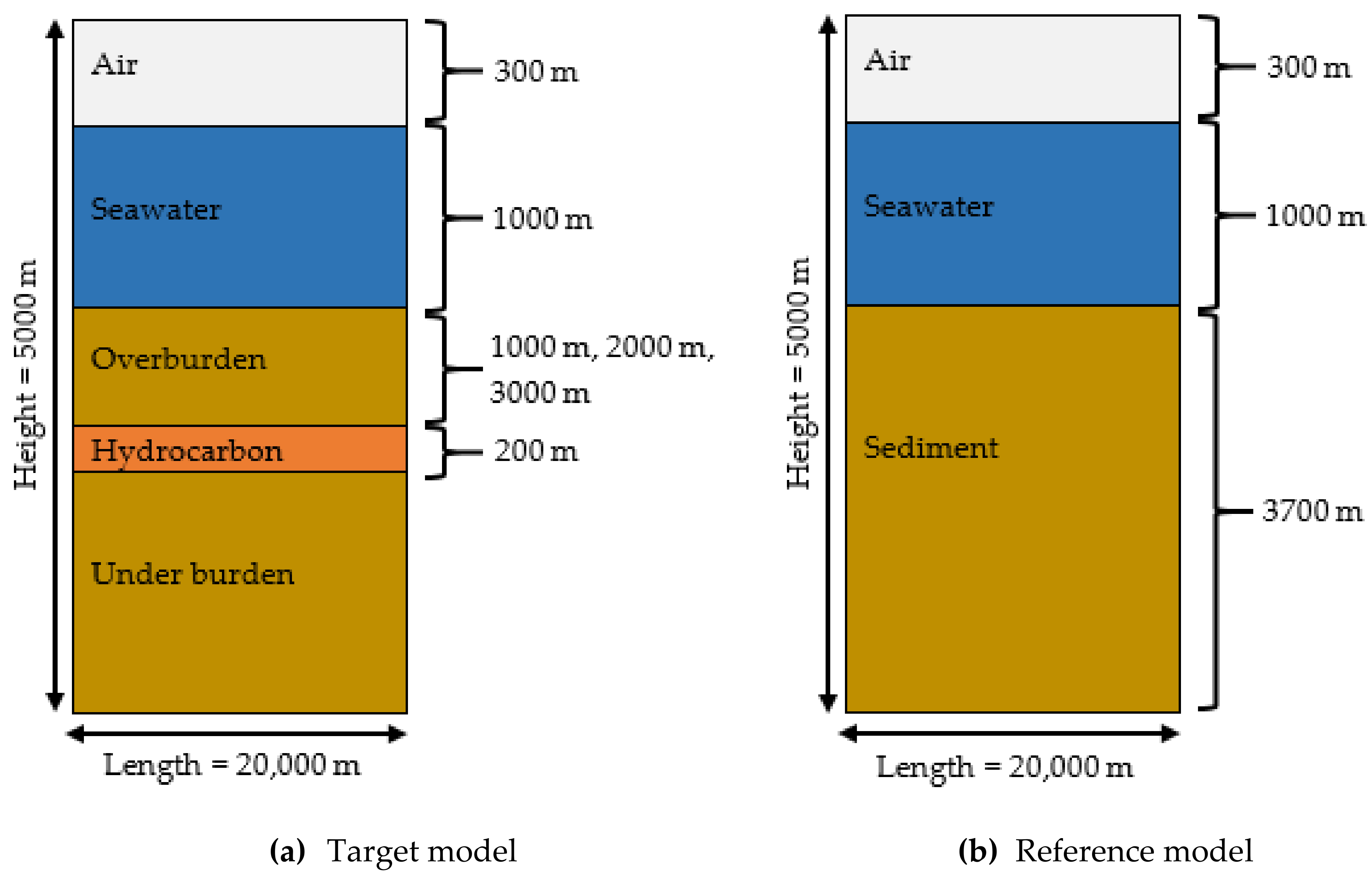
4. Results and Discussion

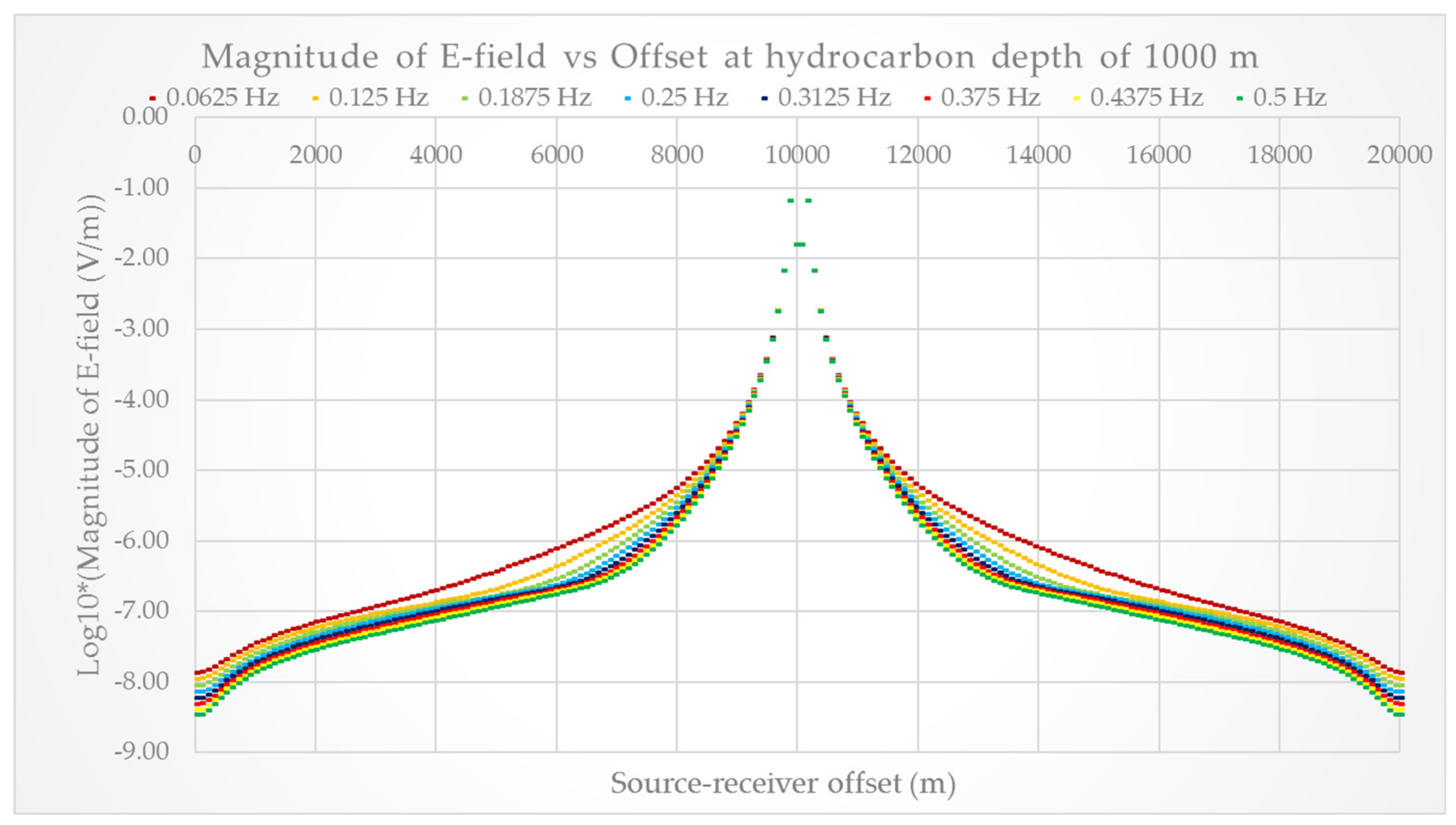
The GP algorithms used in this paper was the GPML Matlab Code version 4.2 (2018) written by Rasmussen, C.E. and Nickisch, H. which can be found in [41]. This research work considered the static source-receiver separation distance phenomenon in the SBL modelling where the transmitter was kept stationary at the center of the SBL models. Here, for the target model, we exercised eight (8) different frequencies (0.0625–0.5 Hz with an increment of 0.0625 Hz) at three (3) different depths of hydrocarbon (1000 m, 2000 m, and 3000 m from the seabed) to acquire the prior information. At every hydrocarbon depth, there were eight datasets which represented EM responses from the target models. The CST computer outputs (i.e., EM responses from target models) for all tested frequencies are depicted in Figure 3, Figure 4 and Figure 5.

Figure 3, Figure 4 and Figure 5 showed the magnitude of the corresponding horizontal E-field for three different overburden thicknesses and eight tried low transmission frequencies. Logarithmic scale with base 10 was applied on the y-axis to make the data more interpretable. Total computation simulation time for the CST software to compute all the 24 datasets of the EM responses (i.e., eight datasets for each hydrocarbon depth) was approximately 90 min (~1 h and 30 min). The CST computer outputs were in good agreement with the trend of real-field EM responses. The strength of the magnitude of E-field decreases as source-receiver separation distance is further apart. Furthermore, E-field strength also decreases as hydrocarbon depth increases. Since the data were acquired with a source located at the center of the SBL model, the EM responses were symmetrical from 0 m to 10,000 m and 10,000 m to 20,000 m. Therefore, we only considered EM responses from 11,000 m to 19,000 m to be processed and fitted by the GP regression (by assuming that the direct wave dominated the first kilometer of the offset from the center). Two-dimensional (2D) forward GP model was developed to provide the information of EM response for all possible frequencies (tried and untried) from 0.0625 Hz to 0.5 Hz at all tested depths of hydrocarbon. The contour plots of EM response were depicted in Figure 6, Figure 7 and Figure 8.

Based on Figure 6, Figure 7 and Figure 8, the x-axis represented source-receiver separation distance (i.e., offset) and the y-axis represented multi-low-frequency (0.0625–0.5 Hz). The log10 of the magnitudes of the E-field are represented and differentiated by the various color codes. The processing time to acquire these three contour plots was less than five (5) minutes with, in total, 45 datasets of EM response being successfully contoured. This shows that the GP model is capable of providing the multi-low-frequency EM information with low time consumption, while the computer simulation could take a few hours to generate those 45 datasets ((8 tried frequencies + 7 untried frequencies) × 3 depths). The tried and untried frequencies at all tested hydrocarbon depths used in the GP methodology are tabulated in

Table 2. Tried and untried frequencies (0.0625–0.5 Hz) for the target models with all hydrocarbon depths. There were 15 datasets of EM response for each depth, hence the total number of datasets were 45. All frequencies employed in this research work were set to have a gap of 0.03125.

Tried Frequency (Hz)	Untried Frequency (Hz)
0.0625	0.09375
0.1250	0.15625
0.1875	0.21875
0.2500	0.28125
0.3125	0.34375
0.3750	0.40625
0.4375	0.46875
0.5000

. As mentioned earlier, eight frequencies were employed in the SBL modelling as observed information. Note that any frequency can be exercised in the GP methodology as the untried transmission frequency as long as the prior knowledge is capable of providing significant information to the GP regression model.

Next, the reliability of the GP model providing the magnitude of the E-field information at the untried transmission frequencies was examined as well. We chose three random untried frequencies between 0.0625 Hz and 0.5 Hz as listed in Table 2 which were 0.09375 Hz, 0.28125 Hz, and 0.46875 Hz in order to identify whether the GP can provide the EM profile at untried/unobserved frequency with adequate accuracy or not. As mentioned before, we exercised three different forecast error measurements, which were MSE, MAD, and MAPE for model validation purposes. The results are tabulated in

Table 3. Forecast error measurement for the three untried transmission frequencies (0.09375 Hz, 0.28125 Hz, and 0.46875 Hz) at all tested depths of hydrocarbon (1000 m, 2000 m, and 3000 m from the seabed).

Frequency (Hz)	HC Depth (m)	MSE	MAD	MAPE (%)
0.09375	1000	0.00025947	0.01158183	0.1737
	2000	0.00003344	0.00319856	0.0421
	3000	0.00006727	0.00454916	0.0592
0.28125	1000	0.00008080	0.00687243	0.1023
	2000	0.00000033	0.00034942	0.0044
	3000	0.00014778	0.00523686	0.0582
0.46875	1000	0.00001381	0.00311347	0.0458
	2000	0.00000237	0.00104498	0.0128
	3000	0.00001470	0.00206036	0.0216

.

Based on Table 3, the MSE, MAD, and MAPE revealed very small values and percentages at all three untried frequencies. On average, the resulting MSE and MAD values were approximately ~0.000069 and ~0.0042, respectively, while the average of MAPE was approximately 0.06% (which is <0.1%). These results indicated that data estimated by the GP were reliable and fit well with the CST outputs even though for the untried/unobserved frequencies. After validating the 2D GP models, the average percentage difference was calculated to compare the trend of the EM responses obtained from the SBL model with the presence of hydrocarbon (target model) and the EM responses obtained from the model without a hydrocarbon layer (reference model). A high-percentage difference indicates the trend that both EM responses are far apart. This means that there is a significant difference between the target and reference EM responses. We used Equation (17) to calculate the average percentage difference (APD):

$$APD=\frac{1}{a}\sum \left[\frac{\left|target response-reference response\right|}{\left(\left|target response\right|-\left|reference response\right|\right)/2}\right]\times 100\%,$$

(17)

where $a$ is the number of data. The histogram depicted in Figure 9 represents the average percentage difference between the target and the reference EM responses for eight (8) transmission frequencies and all tested depths of hydrocarbon.

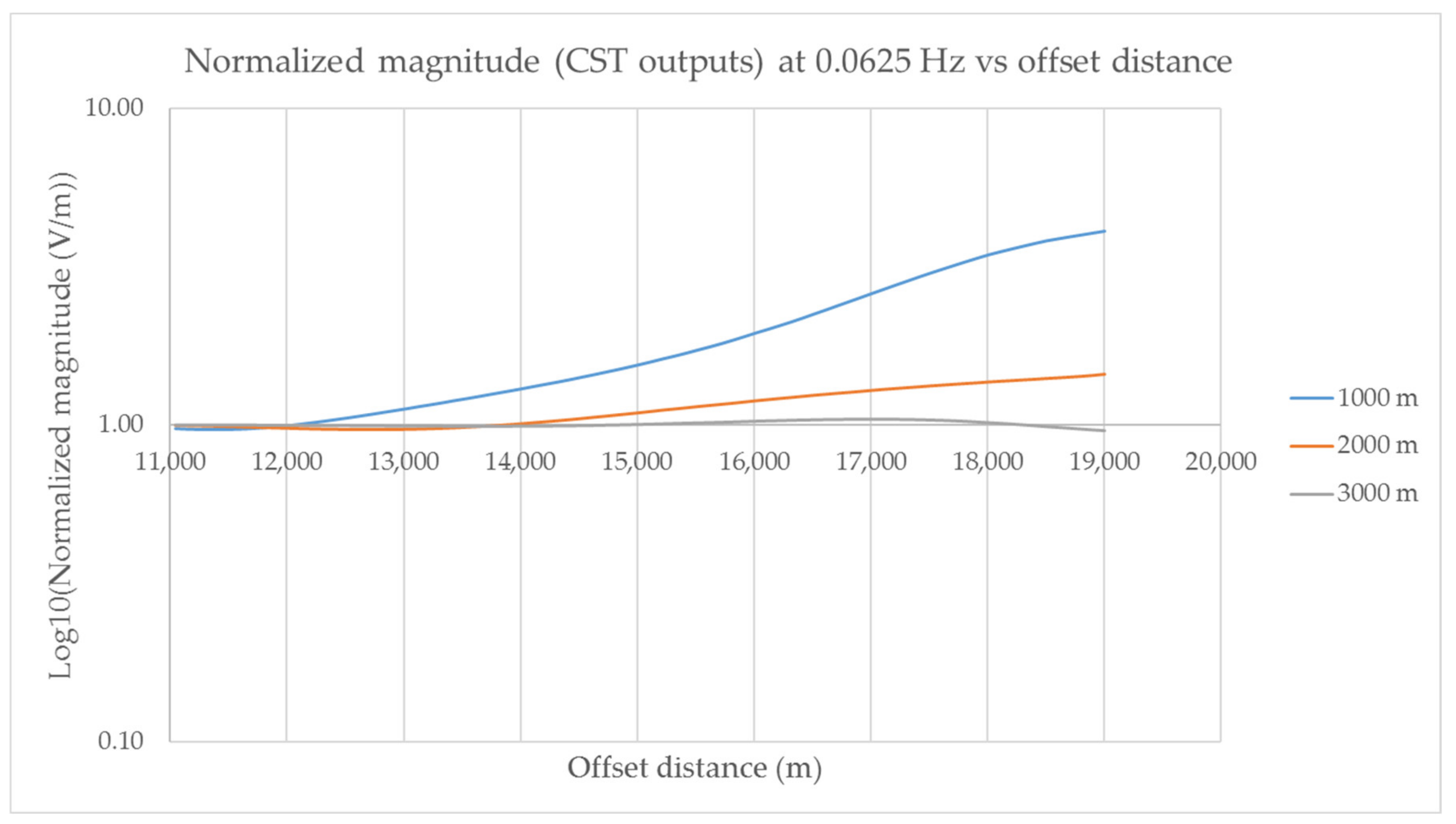
From Figure 9, we can see that, overall, the average percentage differences for the frequency of 0.0625 Hz revealed the smallest percentage for every hydrocarbon depth, while the average percentage differences for 0.5 Hz showed the highest percentage for every hydrocarbon depth. By comparing all the average percentage differences at all depths, a frequency of 0.0625 Hz for the hydrocarbon depth of 3000 m (grey) revealed the smallest APD, which was 0.09%, and a frequency of 0.5 Hz for hydrocarbon at the depth of 1000 m (blue) revealed the highest APD, which was 17.30%. These results indicated that the SBL data between the target and the reference responses become very difficult to understand and analyze as the depth of hydrocarbon increases (assuming that the parameters involved were remained). Hence, the model resolution between these two responses (target and reference) decreased as the hydrocarbon depth increased. Therefore, we provided an MVO analysis by utilizing the 1D GP regression model to quantify the uncertainty. In this part, we only showed MVO plots fitted by the GP for a frequency of 0.0625 Hz (the lowest resulting APD for all depths) to numerically analyze the EM responses, as shown in Figure 10.

Note that the GP model provides predictive variance as an uncertainty quantification. Thus, in this research work, the confidence bar can become an uncertainty quantifier to the MVO analysis whether the hydrocarbon-filled reservoir is significantly present or not. Note that the hydrocarbon-filled reservoir can be inferred as present if variances between the fitted target and the reference responses are not overlapping with each other. Based on Figure 10, the target and the reference EM responses for a frequency of 0.0625 Hz were very difficult to distinguish when hydrocarbon was 3000 m from the seabed. Since the EM trend and 95% confidence intervals of the EM responses were unclear and difficult to interpret, especially for distinguishing the target response at a depth of 3000 m and the reference model, we provided a zoomed-in scale of the variance for all the fitted EM responses shown in Figure 10. This is depicted in Figure 11.

Based on Figure 11, there were four fitted EM responses indicating the three target responses (for hydrocarbon depths of 1000 m, 2000 m, and 3000 m) and one reference response for a frequency of 0.0625 Hz. By referring to the figure, we can see that the EM responses at a hydrocarbon depths of 1000 m and 2000 m with the reference response were certainly comparable and can be distinguished since the variance of each 1D GP model did not overlap each other. However, at this frequency, it was very difficult to distinguish the SBL data between the target response at a hydrocarbon depth of 3000 m and the reference response. Based on the observation from the fitted 1D GP model (red-colored and magenta-colored curves), we can certainly claim that these responses were distinguishable until at source-receiver offset of approximately less than 18,000 m (<~8 km from the source). At an offset of ~18,000 m or more (~18,000 m–20,000 m), EM responses from the reference model suddenly become higher than the target EM responses. Hence, the EM responses become irrelevant and the confidence bars overlapped each other. From this result, for a frequency of 0.0625 Hz, the predictive variance numerically strengthened the claim that the presence of the hydrocarbon reservoir at a hydrocarbon depth of 3000 m was very difficult to identify at a far source-receiver offset and, hence, the model resolution can become very low at these far offsets. Next, we also studied the anomaly trend obtained from the normalized MVO for a frequency of 0.0625 Hz whether the trend is in good agreement with the resulting predictive variance (depicted in Figure 10 and Figure 11) or not, especially when the depth of the hydrocarbon is 3000 m. Therefore, we provided the normalized MVO plot for a frequency of 0.0625 Hz (the lowest tried frequency). This is depicted in Figure 12.

From Figure 12, we can see that these three normalized responses showed anomalies where the responses increase gradually as the source-receiver offsets are further apart. The anomalies can be clearly seen when the offset distance was more than ~12,000 m (>~2 km from the source) for the blue-colored response and more than ~14,000 m (>~4 km from the source) for the reddish-yellow-colored response. However, the anomaly of the normalized response at a hydrocarbon depth of 3000 m seemed not as significant when compared to the other two normalized responses. The grey-colored response showed an irrelevant trend of the normalized magnitudes at far offset distances (>~17,500 m) where the normalized magnitudes suddenly decreased at these offsets. This means that when hydrocarbon was at 3000 m and above, it was very difficult to understand the anomaly at the far offsets even though the lowest transmission frequency (0.0625 Hz) was used. This result is in good agreement with the results in Figure 10 and Figure 11 (using the GP regression model).

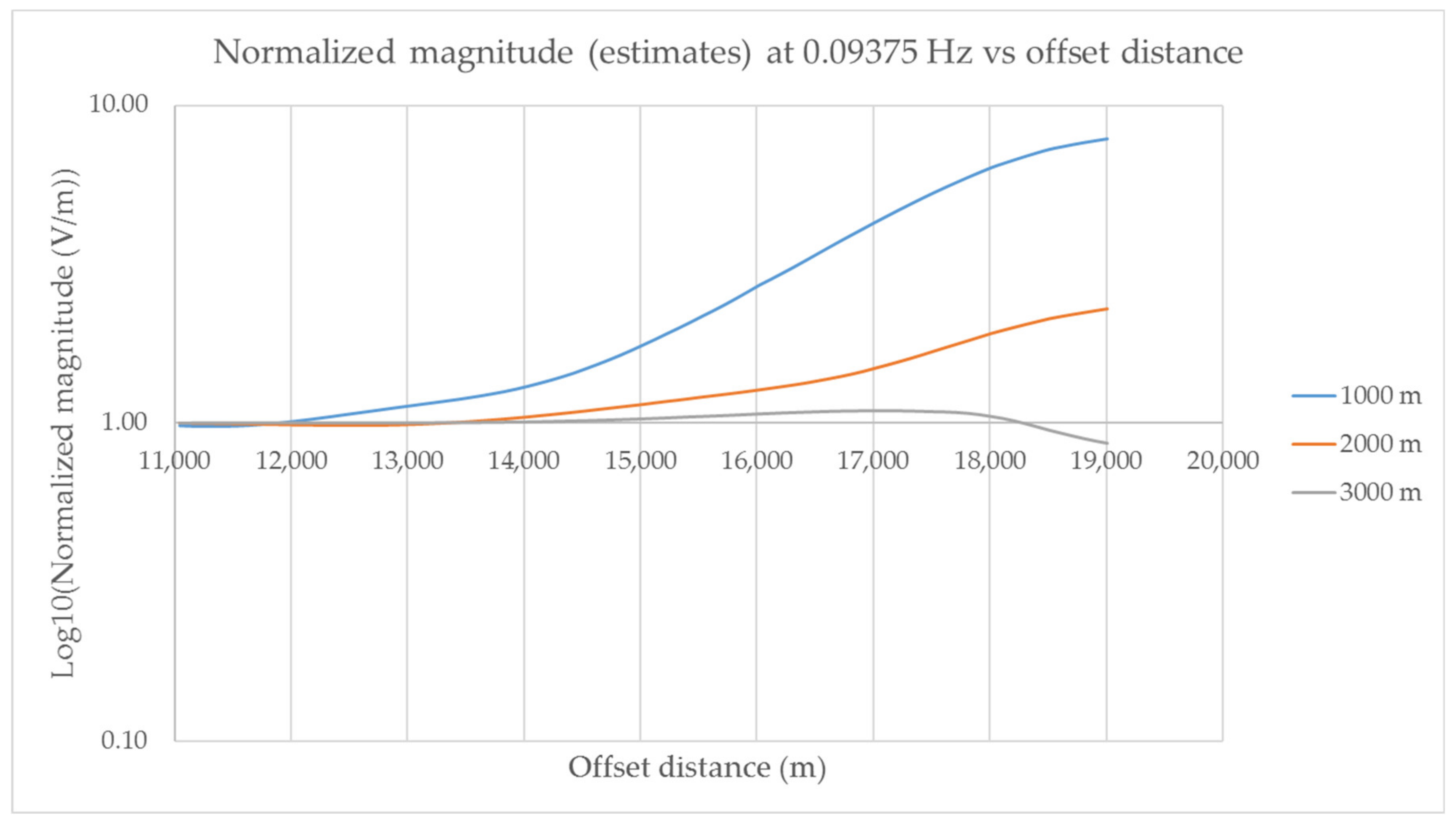
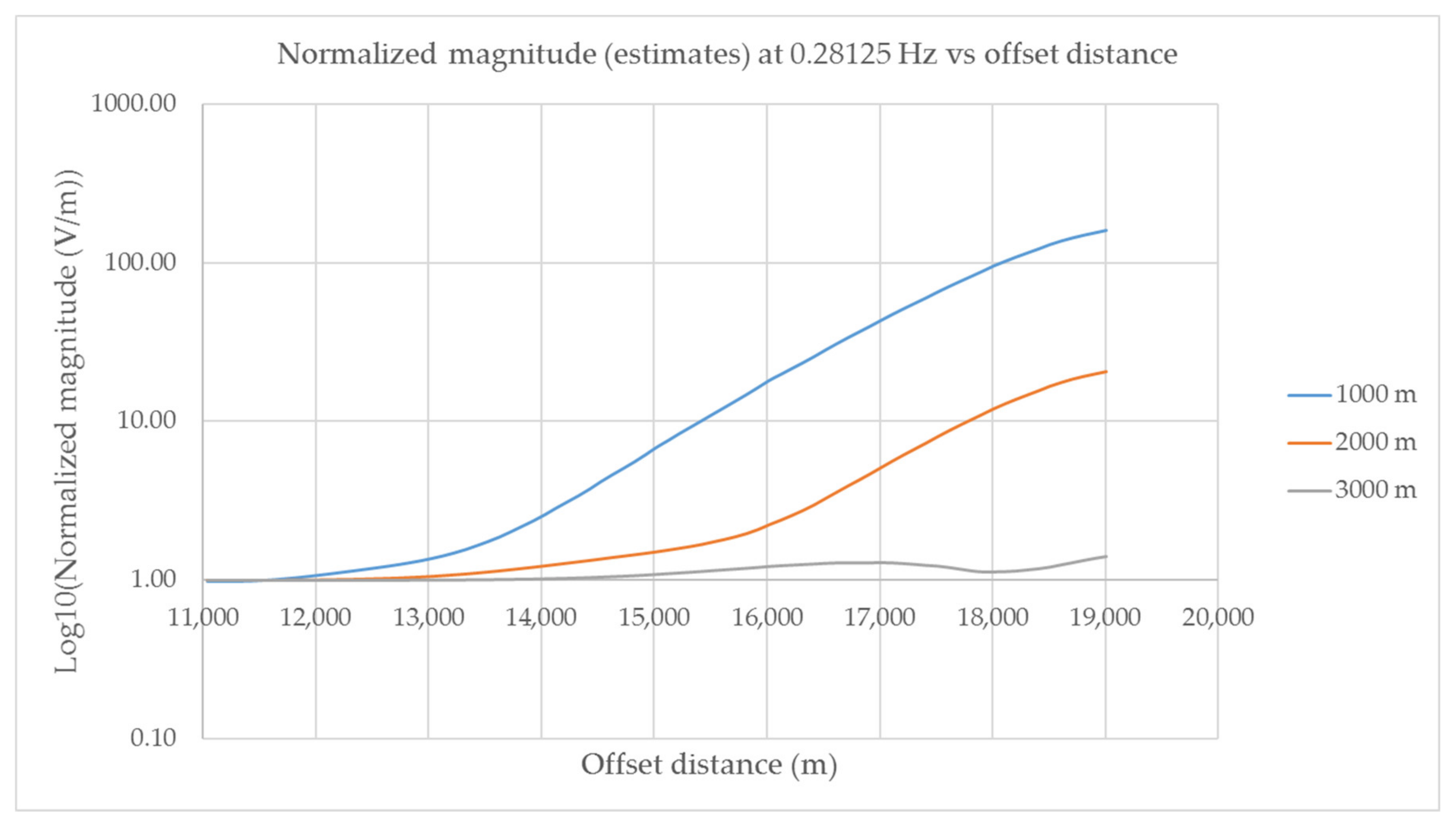
Here, we continued to study the anomaly trend of the normalized MVO for the untried transmission frequencies (0.09375 Hz, 0.28125 Hz, and 0.46875 Hz) by utilizing the developed 2D GP models. Since the estimated EM responses have been validated in the previous section, we utilized the MVO responses in the 2D GP models at all depths of hydrocarbon, which are 1000 m, 2000 m, and 3000 m. This is one of the advantages of this GP methodology where any EM response at any transmission frequency could be used and utilized beforehand for in-depth analysis to understand the responses and acquire the best model resolution for hydrocarbon detection in SBL applications. The normalized magnitudes for those three untried frequencies are depicted in Figure 13, Figure 14 and Figure 15.

Based on Figure 13, Figure 14 and Figure 15, the x-axis represents the offset distance, while the y-axis represents the log10 of the normalized magnitudes at three different depths of hydrocarbon for a transmission frequency of 0.0625 Hz. Here, we can see that anomalies were present in the normalized magnitudes for all three selected untried transmission frequencies as well. Note that all the SBL models were free from any obstructions and noises. Thus, the normalized magnitudes should increase gradually as the offset distance increased. However, based on Figure 13, Figure 14 and Figure 15, the normalized magnitudes at a hydrocarbon depth of 3000 m for all the untried frequencies become irrelevant at far source-receiver offset distances (>~17,500 m). The magnitudes suddenly decrease after gradually increasing from the start (from the source). From these results, we can infer that when the hydrocarbon depth was at 3000 m and above beneath the seabed, hydrocarbon anomalies were difficult to interpret at far source-receiver separation distances even though multi-low-frequencies (0.0625 Hz–0.5 Hz) were employed in the SBL application.

5. Conclusions

We presented an MVO analysis of the EM surveying technique by calibrating models from the stochastic process (Gaussian process regression) and the computer experiment (CST computer outputs). 2D GP models were developed to provide information of multi-low-frequency EM data at various observations (numerous realizations of input-output pairs). Based on the results obtained from the model validation, values of the MSE, MAD, and MAPE revealed that the 2D GP regression was able to model and estimate the EM profile for all the tried and untried transmission frequencies at three different depths of hydrocarbon. The processing time and the reliability of the GP providing the EM profile information proved that this model calibration was an efficient methodology. Next, the predictive variance with a 95% confidence interval certainly showed that target responses from hydrocarbon depths of 1000 m and 2000 m and the reference response were distinguishable at the lowest tried frequency, which was 0.0625 Hz. However, confidence bars between the target response from a hydrocarbon depth of 3000 m and the reference response from a frequency of 0.0625 Hz overlapped each other at the far source-receiver offsets. Results from the normalized magnitudes for the tried frequency (0.0625 Hz) and untried frequencies (0.09375 Hz, 0.28125 Hz, and 0.46875 Hz) also were in good agreement with the resulting predictive variance. This concluded that the model resolution of the MVO plots at a hydrocarbon depth of 3000 m was low at the offset distance of more than ~17,500 m (>~7.5 km from the source) even though multiple low frequencies were employed in the survey. Coming to a deeper hydrocarbon-filled situation, in-depth analysis is required before any decision-making is made. Therefore, this attempt may help the EM imaging by providing additional and beneficial information to the scanning or risk analysis with low time-consumption for better model resolution of subsurface modelling in SBL applications.

References

1. Børven, J.M.; Flekkøy, E.G. New EM technology uses vertical rather than horizontal electrical lines. World Oil 2009, 230, 41–45. [Google Scholar]
2. Eidesmo, T.; Ellingsrud, S.; MacGregor, L.M.; Constable, S.; Sinha, M.C.; Johansen, S.; Kong, F.N.; Westerdahl, H. Sea Bed Logging (SBL), a new method for remote and direct identification of hydrocarbon filled layers in deep water areas. First Break 2002, 20, 144–152. [Google Scholar]
3. Ellingsrud, S.; Eidesmo, T.; Johansen, S. Remote sensing of hydrocarbon layers by seabed logging: Results from a cruise offshore Angola. Lead. Edge 2002, 21, 972–982. [Google Scholar] [CrossRef]
4. Srnka, L.J.; Carazzone, J.J.; Ephron, M.S.; Eriksen, E.A. Remote reservoir resistivity mapping. Lead. Edge 2006, 25, 972–975. [Google Scholar] [CrossRef]
5. Dunham, M.W.; Ansari, S.M.; Farquharson, C.G. Application of 3D Marine CSEM Finite-Element Forward Modeling to Hydrocarbon Exploration in the Flemish Pass Basin Offshore Newfoundland, Canada. In Proceedings of the SEG International Exposition and 86th Annual Meeting, Dallas, TX, USA, 16–21 October 2016; pp. 917–921. [Google Scholar]
6. Li, Y.; Key, K. 2D marine controlled-source electromagnetic modeling: Part 1—An adaptive finite-element algorithm. Geophysics 2007, 75, WA51–WA62. [Google Scholar] [CrossRef]
7. Bakr, S.A.; Pardo, D.; Mannseth, T. Domain decomposition Fourier finite element method for the simulation of 3D marine CSEM measurements. J. Comput. Phys. 2013, 255, 456–470. [Google Scholar] [CrossRef]
8. Sengupta, S. Target Detectability of Marine Controlled Source Electromagnetic Method—Insights from 1-D modeling. In Proceedings of the 2nd South Asian Geoscience Conference and Exhibition, GEO India 2011, New Delhi, India, 12–14 January 2011; Available online: https://apgindia.org/document/704.pdf (accessed on 6 March 2020).
9. Aris, M.N.M.; Daud, H.; Dass, S.C.; Noh, K.A.M. Gaussian processes for hydrocarbon depth estimation in forward modeling of seabed logging. J. Environ. Eng. Geophys. 2019, 24, 399–408. [Google Scholar]
10. Mohd Aris, M.N.; Daud, H.; Dass, S.C.; Mohd Noh, K.A. Gaussian process methodology for multi-frequency marine controlled-source electromagnetic profile estimation in isotropic medium. Processes 2019, 7, 661. [Google Scholar] [CrossRef] [Green Version]
11. Kee, R.J.; Grcar, J.F.; Smooke, M.D.; Miller, J.A.; Meeks, E. A FORTRAN Program for Modeling Steady Laminar One-Dimensional Premixed Flames; Sandia Report SAND85-8240; National Technical Information Service: Springfield, MO, USA, 1985. [Google Scholar]
12. Sacks, J.; Welch, W.; Mitchell, T.; Wyan, H.P. Design analysis of computer Experiments. Stat. Sci. 1989, 4, 409–423. [Google Scholar] [CrossRef]
13. Harari, O.; Steinberg, D.M. Optimal designs for Gaussian process models |via spectral decomposition. J. Stat. Plan. Inference 2014, 154, 87–101. [Google Scholar] [CrossRef]
14. Santner, T.; Williams, B.; Nolts, W. The Design and Analysis of Computer Experiments; Springer: Berlin/Heidelberg, Germany, 2003. [Google Scholar]
15. Trucano, T.G.; Pilch, M.; Oberkampf, W.L. General Concepts for Experimental Validation of ASCI Code Applications; Technical Report SAND2002-0341; Sandia National Laboratories: Albuquerque, NM, USA, 2002. [Google Scholar]
16. Higdon, D.; Gattiker, J.; Williams, B.; Rightley, M. Computer model calibration using high dimensional output. J. Am. Stat. Assoc. 2008, 103, 570–583. [Google Scholar] [CrossRef] [Green Version]
17. Hills, R.G.; Trucano, T.G. Statistical Validation of Engineering and Scientific Models: Background; SAND99-1256; Sandia National Laboratories: Albuquerque, NM, USA, 1999. [Google Scholar]
18. Hills, R.G.; Trucano, T.G. Statistical Validation of Engineering and Scientific Models: A Maximum Likelihood Based Metric; SAND2001-1783; Sandia National Laboratories: Albuquerque, NM, USA, 2002. [Google Scholar]
19. Hills, R.G. Model validation: Model parameter and measurement uncertainty. J. Heat Transf. 2006, 128, 339–351. [Google Scholar] [CrossRef]
20. Wang, S.; Chen, W.; Tsui, K.L. Bayesian validation of computer models. Technometrics 2009, 51, 439–451. [Google Scholar] [CrossRef]
21. Schwaighofer, A.; Tresp, V. Transductive and inductive methods for approximate Gaussian process regression. In Advances in Neural Information Processing Systems; MIT Press: Cambridge, MA, USA, 2003. [Google Scholar]
22. Chan, L.L.T.; Liu, Y.; Chen, J. Nonlinear system identification with selective recursive Gaussian process models. Ind. Eng. Chem. Res. 2013, 52, 18276–18286. [Google Scholar] [CrossRef]
23. Rasmussen, C.E.; Nickisch, H. Gaussian Processes for Machine Learning (GPML) Toolbox. J. Mach. Learn. Res. 2010, 11, 3011–3015. [Google Scholar]
24. Gibson, N.P.; Aigrain, S.; Roberts, S.; Evans, T.M.; Osborne, M.; Pont, F. A Gaussian process framework for modelling instrumental systematics: Application to transmission spectroscopy. Mon. Not. R. Astron. Soc. 2012, 419, 2683–2694. [Google Scholar] [CrossRef]
25. Pal, M.; Deswal, S. Modelling pile capacity using Gaussian process regression. Comput. Geotech. 2010, 37, 942–947. [Google Scholar] [CrossRef]
26. Yin, F.; Zhao, Y.; Gunnarsson, F.; Gustafsson, F. Received-Signal-Strength Threshold Optimization Using Gaussian Processes. IEEE Trans. Signal Process. 2017, 65, 2164–2177. [Google Scholar] [CrossRef] [Green Version]
27. Liu, D.; Pang, J.; Zhou, J.; Peng, Y.; Pecht, M. Prognostics for state of health estimation of lithium-ion batteries based on combination Gaussian process functional regression. Microelectron. Reliab. 2013, 53, 832–839. [Google Scholar] [CrossRef]
28. Wang, H.; Gao, X.; Zhang, K.; Li, J. Fast single image super-resolution using sparse Gaussian process regression. Signal Process. 2017, 134, 52–62. [Google Scholar] [CrossRef]
29. Chen, J.; Yu, J.; Zhang, Y. Multivariate video analysis and Gaussian process regression model based soft sensor for online estimation and prediction of nickel pellet size distributions. Comput. Chem. Eng. 2014, 64, 13–23. [Google Scholar] [CrossRef]
30. Asante-Okyere, S.; Shen, C.; Ziggah, Y.Y.; Rulegeya, M.M.; Zhu, X. Investigating the predictive performance of Gaussian process regression in evaluating reservoir porosity and permeability. Energies 2018, 11, 3261. [Google Scholar] [CrossRef] [Green Version]
31. Teflove, A.; Hagness, S.C. Computational Electrodynamics: The Finite-Difference Time-Domain Method; Artech House: Boston, MA, USA; London, UK, 2005. [Google Scholar]
32. Daud, H.; Razali, R.; Asirvadam, V. Sea bed logging applications: Predicting hydrocarbon depth using mathematical equations. Appl. Mech. Mater. 2015, 789, 560–565. [Google Scholar] [CrossRef]
33. Daud, H.; Sagayan, V.A.; Razali, R.; Talib, M. Distinguishing data with and without hydrocarbon in scale tank experiments using spline interpolation and normalized mean square error. AIP Conf. Proc. 2014, 1605, 268–273. [Google Scholar]
34. Yahya, N.; Nasir, N.; Akhtar, M.N.; Kashif, M.; Mohd Zaid, H.; Shafie, A. Modeling of antenna for deep target hydrocarbon exploration. J. Electromagn. Anal. Appl. 2012, 4, 30–41. [Google Scholar] [CrossRef] [Green Version]
35. Rauf, M.; Yahya, N.; Nyamasvisva, T.E.; Ansari, A.; Shafie, A.; Nahar, N. Prediction of double stacking hydrocarbon using marine controlled source electromagnetic method. In Proceedings of the IEEE Asia-Pacific Conference on Applied Electromagnetics (APACE 2014), Johor, Malaysia, 8–10 December 2014. [Google Scholar]
36. Mukhtar, S.M.; Daud, H.; Dass, S.C. Prediction of hydrocarbon using Gaussian process for seabed logging application. Procedia Comput. Sci. 2015, 72C, 225–232. [Google Scholar] [CrossRef] [Green Version]
37. Ansari, A.; Shafie, A.B.; Said, A.B. Relationship of resistivity contrast and thickness depth of hydrocarbon for seabed logging application. Int. J. Comput. Sci. 2012, 9, 214–221. [Google Scholar]
38. Aris, M.N.M.; Daud, H.; Dass, S.C. Prediction of hydrocarbon depth for seabed logging (SBL) application using Gaussian process. J. Phys. Conf. Ser. 2018, 1132, 012075. [Google Scholar] [CrossRef]
39. Mohd Aris, M.N.; Daud, H.; Dass, S.C. Processing synthetic seabed logging (SBL) data using Gaussian Process regression. Phys. Conf. Ser. 2018, 1123, 012025. [Google Scholar] [CrossRef]
40. CST STUDIO SUITE Electromagnetic Field Simulation Software. Available online:https://www.3ds.com/products-services/simulia/products/cst-studio-suite/ (accessed on 15 July 2019).
41. Rasmussen, C.E.; Nickisch, H. Documentation for GPML Matlab Code Version 4.2. Available online: http://www.gaussianprocess.org/gpml/code/matlab/doc/ (accessed on 1 October 2019).
Figure 1. Stratified illustration of the SBL models. There are two types of SBL models: (a) SBL model with the presence of hydrocarbon layer; (b) SBL model without the hydrocarbon layer. For the target model, depth of the hydrocarbon (thickness of overburden) was varied, which were 1000 m, 2000 m, and 3000 m. The height and length of both the SBL models were 5000 m and 20,000 m, respectively.
Processes 08 00605 g001
Figure 2. Simplified methodological flow of GP regression modelling in SBL data generated through the CST software.
Processes 08 00605 g002
Figure 3. EM responses obtained from the target models, where the hydrocarbon layer was located at 1000 m from the seabed, for multiple frequencies (0.0625–0.5 Hz with an increment of 0.0625 Hz each). The total source-receiver separation distance is 20,000 m.
Processes 08 00605 g003
Figure 4. EM responses obtained from the target models, where the hydrocarbon layer was located at 2000 m from the seabed, for multiple frequencies (0.0625–0.5 Hz with an increment of 0.0625 Hz each). The total source-receiver separation distance is 20,000 m.
Processes 08 00605 g004
Figure 5. EM responses obtained from the target models, where the hydrocarbon layer was located at 3000 m from the seabed, for multiple frequencies (0.0625–0.5 Hz with an increment of 0.0625 Hz each). The total source-receiver separation distance is 20,000 m.
Processes 08 00605 g005
Figure 6. Contour plot of the 2D forward GP model. EM responses versus source-receiver separation distance for all tried and untried transmission frequencies (0.0625–0.5 Hz) at overburden thickness of 1000 m.
Processes 08 00605 g006
Figure 7. Contour plot of the 2D forward GP model. EM responses versus source-receiver separation distance for all tried and untried transmission frequencies (0.0625–0.5 Hz) at overburden thickness of 2000 m.
Processes 08 00605 g007
Figure 8. Contour plot of the 2D forward GP model. EM responses versus source-receiver separation distance for all tried and untried transmission frequencies (0.0625–0.5 Hz) at overburden thickness of 3000 m.
Processes 08 00605 g008
Figure 9. Histogram of the average percentage difference between the target EM responses and the reference responses. There were three histograms which represented the depths of hydrocarbon. The average percentage difference was calculated for every transmission frequency used in this research work (0.0625–0.5 Hz with an increment of 0.0625 Hz).
Processes 08 00605 g009
Figure 10. 1D GP models of MVO responses observed along the receiver line from four different SBL models at a frequency of 0.0625 Hz: (i) model with hydrocarbon depth of 1000 m (blue); (ii) model with hydrocarbon depth of 2000 m (green); (iii) model with hydrocarbon depth of 3000 m (red); (iv) model with no hydrocarbon layer (magenta).
Processes 08 00605 g010
Figure 11. Zoomed-in scale of the 1D GP models for a frequency of 0.0625 Hz. The grey-colored bar is the 95% confidence interval (predictive variance) provided by the GP. The “cross” denotes the testing data involved in the GP regression.
Processes 08 00605 g011
Figure 12. Normalized MVO responses for a transmission frequency of 0.0625 Hz observed along the receiver line for three different hydrocarbon depths: (i) normalized MVO for a hydrocarbon depth of 1000 m (blue); (ii) normalized MVO for a hydrocarbon depth of 2000 m (reddish-yellow); (iii) normalized MVO for a hydrocarbon depth of 3000 m (grey).
Processes 08 00605 g012
Figure 13. Normalized MVO responses for transmission frequency of 0.09375 Hz: (i) normalized MVO for a hydrocarbon depth of 1000 m (blue); (ii) normalized MVO for a hydrocarbon depth of 2000 m (reddish-yellow); (iii) normalized MVO for a hydrocarbon depth of 3000 m (grey).
Processes 08 00605 g013
Figure 14. Normalized MVO responses for transmission frequency of 0.28125 Hz: (i) normalized MVO for a hydrocarbon depth of 1000 m (blue); (ii) normalized MVO for a hydrocarbon depth of 2000 m (reddish-yellow); (iii) normalized MVO for a hydrocarbon depth of 3000 m (grey).
Processes 08 00605 g014
Figure 15. Normalized MVO responses for transmission frequency of 0.46875 Hz: (i) normalized MVO for a hydrocarbon depth of 1000 m (blue); (ii) normalized MVO for a hydrocarbon depth of 2000 m (reddish-yellow); (iii) normalized MVO for a hydrocarbon depth of 3000 m (grey).
Processes 08 00605 g015