

Attention-Based Two-Dimensional Dynamic-Scale Graph Autoencoder for Batch Process Monitoring

1
School of Food Science and Technology, Jiangnan University, Wuxi 214122, China
2
School of Artificial Intelligence and Computer Science, Jiangnan University, Wuxi 214122, China
3
Department of Chemical and Biological Engineering, Hong Kong University of Science and Technology, Clear Water Bay, Kowloon, Hong Kong SAR 999077, China
*
Author to whom correspondence should be addressed.
Processes 2024, 12(3), 513; https://doi.org/10.3390/pr12030513
Submission received: 8 February 2024
/
Revised: 27 February 2024
/
Accepted: 29 February 2024
/
Published: 2 March 2024
(This article belongs to the Special Issue Data-Based Process Monitoring, Process Control, and Quality Improvement in Industry)
Abstract
:Traditional two-dimensional dynamic fault detection methods describe nonlinear dynamics by constructing a two-dimensional sliding window in the batch and time directions. However, determining the shape of a two-dimensional sliding window for different phases can be challenging. Samples in the two-dimensional sliding windows are assigned equal importance before being utilized for feature engineering and statistical control. This will inevitably lead to redundancy in the input, complicating fault detection. This paper proposes a novel method named attention-based two-dimensional dynamic-scale graph autoencoder (2D-ADSGAE). Firstly, a new approach is introduced to construct a graph based on a predefined sliding window, taking into account the differences in importance and redundancy. Secondly, to address the training difficulties and adapt to the inherent heterogeneity typically present in the dynamics of a batch across both its time and batch directions, we devise a method to determine the shape of the sliding window using the Pearson correlation coefficient and a high-density gridding policy. The method is advantageous in determining the shape of the sliding windows at different phases, extracting nonlinear dynamics from batch process data, and reducing redundant information in the sliding windows. Two case studies demonstrate the superiority of 2D-ADSGAE.
1. Introduction
In recent decades, batch processes have been widely used in manufacturing products, which are indispensable in the modern landscape, ranging from food and pharmaceuticals to the most cutting-edge silicon [1]. The overall normal operation of a specific batch process is essential for the concern of safety and profitability, and plays a central role in the ultimate success of a process [2,3,4]. To this end, process monitoring is now an increasingly studied topic in batch process systems and has been improved by the great surge in data from real-world operations. Particularly, statistical process control (SPC), as an emerging technique, has found widespread applications in the field of process monitoring [5,6,7,8].
Generally, SPC attempts to monitor the data by mining the stable and event-sensitive patterns underlying the data, instead of relying on the complex process knowledge that is hard to obtain in practice. Due to this unique advantage, multivariate principal component analysis (MPCA) and multivariate partial least squares (MPLS) have been extensively used for fitting the cross- and auto-relations in the input data, which is also referred to as the issue of nonlinearities and dynamics underlying batch processes [9,10].
Actually, in real-world batch processes, there is a correlation between process data and historical data [11]. Batch processes are typically dynamic in nature due to the chronological generation of process data [12]. This results in the existence of nonlinear dynamics that not only reside in the time dimension but also in the batch dimension. To extract batch process data dynamics, researchers have successfully combined data augmentation techniques and SPC models, proposing the dynamic principal component analysis (DPCA) and dynamic kernel principal component analysis [13,14,15]. However, these kind of approaches only consider correlations in the time dimension. Meanwhile, some researchers tried to construct 2D batch process monitoring models. Lu [16] proposed a 2D sliding window in the time and batch directions and combined the sliding window with DPCA to capture the dynamic characteristics of the batch process. This approach assumes that 2D sliding windows are regular, whereas certain batch process dynamics may not be represented using regular sliding windows. For the determination of the shape of the sliding window, many different methods have been proposed by researchers. Yao [17] proposed a method called region of support (ROS) to extract the dynamics of the batch process. The shape of the sliding window has been further defined with the support of ROS and this sliding window has an irregular shape. Jiang [18] proposed a 2D-DCRL model and used DCCA to compute the correlation of samples in the time and batch dimensions to finalize the shape of the sliding window. Unlike the methods mentioned above, Ren [19] performed data augmentation by sliding a window along the batch direction on the batch process data and then processed the data using an autoencoder based on a long short-term memory network to monitor the batch process.
The aforementioned 2D methods reshape sample data into a new matrix via specific regions or sliding windows, which is subsequently utilized for model training. However, these methods overlook the possibility of redundancy among samples within the sliding window. The determination of the sliding window’s shape in these methods is based on calculating the correlation between samples using a linear approach. Although these methods can select samples that are highly correlated with the current sample to form a 2D sliding window, this linear correlation may bring redundant information into the model. This redundancy is also reflected in the fact that the model assumes that all samples in the sliding window are of equal importance, which does not take full advantage of the correlation between the samples. In addition, neither the regular sliding windows nor the shaped sliding windows identified by data mining take into account the variation in the shape of the sliding window with respect to the time direction of the batch process. As a single batch process typically encompasses multiple phases characterized by distinct dynamics, it becomes necessary to adapt the sliding window’s configuration to align with the specific characteristics of each phase.
With the continual advancement in graph neural networks, graph-based neural network models have garnered significant attention in domains such as natural language processing and computer vision [20,21]. Particularly, graph models can use correlations between data to construct edges in a graph to extract structural information from the data [22,23]. Therefore, researcher have tried to apply graph neural network modeling to process monitoring. Zhang [24] introduced the pruning graph convolutional network (PGCN) model for fault diagnosis, pioneering the fusion of a graph convolution network (GCN) with one-dimensional industrial process data. Liu [25] determined the shape of a one-dimensional sliding window by analyzing sample autocorrelation. They constructed a graph using a sliding window and used a graph convolutional network for information aggregation and updating to reduce the dimension and reconstruct the original input. Moreover, the graph attention network (GAT) [26], a classical model in the field of graph neural networks, demonstrates a remarkable capacity to extract vital information from raw data. This proficiency is attributed to the self-attention mechanism employed by GAT. By leveraging the graph structure, the self-attention mechanism efficiently filters out crucial information within the graph. It accomplishes this by computing attention weights for each node and its neighboring nodes, thereby mitigating the influence of redundant information on the model. Hence, GAT is more advantageous in extracting key information and reducing the interference of redundant information.
For those reasons, this paper proposes a new batch process monitoring method named attention-based two-dimensional dynamic-scale graph autoencoder (2D-ADSGAE), which combines GAT and SAE to construct an effective dynamic batch process monitoring model. In this work, the batch process is divided into different phases according to our proposed phase division method to determine the shape of the 2D sliding window at each phase, and then the normalized batch process data are used to construct the graph. The 2D-ADSGAE is a network with an encoder–decoder architecture, comprising multiple GAT layers. This method further extracts crucial information from the graph through attention mechanisms, reducing the impact of redundant information on the model. Network parameters are optimized by minimizing the reconstruction loss. Finally, a fault diagnosis method based on a deep reconstruction-based contribution (DRBC) plot is proposed to locate the fault variables and estimate the fault magnitude when a fault is detected. The contributions of this research are summarized as follows:
- We devise a way to expound the heterogeneity of process dynamics that a batch process typically has across its time and batch direction, showcasing the necessity of updating receptive regions and assuaging redundancy for feature engineering.
- Multi-phase sliding windows are utilized to construct the batch process data into a single graph with varying structures that are suitable for a graph neural networks-based model.
- Additionally, the model’s practical applicability is demonstrated by analyzing the root cause of the faults through a comparison of the loss between inputs and reconstructions.
2. Preliminaries
2.1. Graph Attention Network
The graph attention network, introduced in 2017 as an alternative to the graph convolution network, has demonstrated satisfactory performance on established node classification datasets [26]. Unlike traditional approaches, GAT does not require intricate matrix operations or prior graph knowledge. Instead, it manages neighborhoods of varying sizes through self-attention layers, dynamically assigning attention weights to distinct nodes within the neighborhood during the update phase. The GAT mechanism operates as follows.
First, a set of graph node features, denoted as H =, , is input. Second, the attention score of node is computed considering all neighboring nodes. Finally, the features of neighboring nodes are weighted and aggregated using these attention scores to derive the updated feature of node .
where W is a shared linear transform weight matrix and denotes the neighbors of the node. is a single-layer feed-forward neural network. represents the activation function ReLU.
2.2. Stacked Autoencoder
The SAE is an amalgamation of multiple autoencoders (AEs). As illustrated in Figure 1a, AE consists of an input layer, a hidden layer, and an output layer. Its purpose is to extract hidden features from high-dimensional data and train neural network parameters using the reconstruction loss. This metric is updated via backpropagation. Let the input of AE , where is the feature dimension of the input samples and n is the number of samples. When input into the encoder, is transformed into through the application of the nonlinear activation function , where d represents the feature dimension of the hidden layer. This process is expressed in Equation (4).
where is the nonlinear variation weight matrix of the encoder and is the bias. When decoding, the decoder employs the nonlinear activation function to reconstruct as . Both and share the same dimension . The reconstruction process can be depicted as follows.
where is the weight matrix and is the bias vector of the decoder. Usually, the reconstruction loss is used as a training metric for AE. The reconstruction loss of AE can be represented by the following Equation (6).
As previously mentioned, the SAE comprises multiple AEs integrated into a unified structure, as illustrated in Figure 1b. Each AE layer’s output within the SAE serves as the subsequent AE layer’s input, thereby forming a larger encoder–decoder architecture. During the pre-training phase, a greedy approach is employed to train each AE layer individually. However, the locally optimal performance achieved by the greedy algorithm across each AE layer does not necessarily represent the global optimum. Consequently, after pre-training all the AEs, the comprehensive fine-tuning of the entire SAE becomes imperative to attain model parameters conducive to the global optimal performance. Both the pre-training and fine-tuning stages of the SAE leverage backpropagation and gradient descent algorithms to optimize the model parameters. The 2D-ADSGAE, proposed in this paper, adheres to a similar training strategy as the SAE.
3. Methodology
3.1. Preprocessing on Batch Process Data
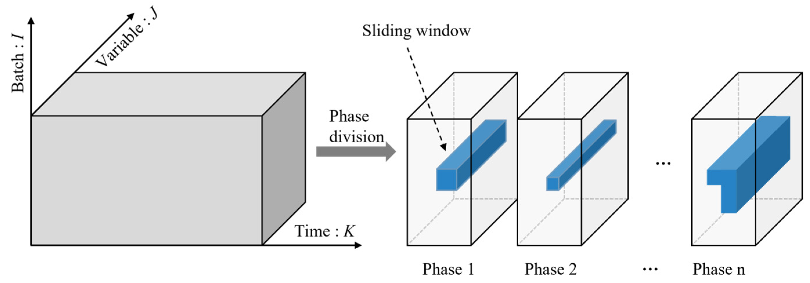
In contrast to the two-dimensional data format involving time and process variables in continuous processes, batch process data consolidates information collected from multiple batches, forming a three-dimensional tensor , where I, J, and K indicate the number of batches, variables, and samples, respectively [27]. Before modeling, we normalized the batch process data. Initially, X was unfolded into a two-dimensional matrix , and subsequently, each variable was standardized using Z-score. Then, we divided the tensor X into A initial phases, with each phase having the same shape of .
In order to capture the 2D dynamic features, different 2D sliding windows were used in each phase, as shown in Figure 2. Figure 3 illustrates the details of the 2D sliding window. Each window was composed of samples from the current sample and from previous time and batch directions. First, the initial window shape was set to , where is the time order and is the batch order. Second, we calculated the Pearson correlation between samples in the sliding window, as summarized in Algorithm 1, and then selected the sliding window with the largest average correlation coefficient as the initial sliding window of all phases. After this, we computed the Pearson correlation coefficient for the sliding window among adjacent phases and merged those phases exhibiting correlation coefficients exceeding 0.7. Finally, we obtained the final solution of the phase division.
An appropriate sliding window shape is crucial when constructing a 2D sliding window. Next, the final shape of the sliding window in each phase was determined. Even though we determined the initial sliding window shape for each phase, optimizing the sliding window shape further is essential to mitigate the interference caused by redundant information. Given the substantial time-series correlation present in batch process data, our initial focus was on the time dimension, for which selecting the appropriate order was our first consideration. First, we calculated the sample correlation in the sliding window through Algorithm 1 for each phase. Then, the final shape of the sliding window was determined through Algorithm 2.
| Algorithm 1. Calculate the correlation of the samples in the sliding windows |
| Require: Batch process data |
| 1: Initial |
| 2: Set the size of sliding window , where |
| 3: for todo |
| 4: for to do |
| 5: for to do |
| 6: for to do |
| 7: Unfold to |
| 8: Unfold to |
| 9: Append into |
| 10: end for |
| 11: end for |
| 12: Calculate correlation matrix of , where |
| 13: for to do |
| 14: for to do |
| 15: ← mean of |
| 16: end for |
| 17: end for |
| 18: end for |
| 19: end for |
| 20: return the sample correlation matrix of the sliding window |
| Algorithm 2. Determine the final shape of the sliding window |
| Require: sample correlation of the sliding window |
| 1: Set |
| 2: find and of each row and column |
| 3: mark , where of each row |
| 4: mark , where of each column |
| 5: The marked part in is the final shape of the sliding window |
| 6: return the shape of the of the sliding window |
Figure 4 illustrates the sample correlations in the window at each phase of the penicillin fermentation process. The initial window shape was set to . From Figure 4a, we can see that there is a strong correlation between the time and batch directions. Figure 4b,c indicate that the correlation in the batch direction gradually becomes weaker, while Figure 4d shows the strong correlation in the batch direction, which is different from Figure 4b,c.
3.2. Description of the 2D-ADSGAE
Inside the window we determined in Section 3.1, each time-specific sample was assumed as an individual node, to be configured in the graph that was used as the input for the model of ADSGAE. The neighbors of each node in the graph were not necessarily confined among the samples in adjacent time and phases, but among all the others captured by the current window.
The weight assigned to each edge within the graph is a crucial factor. The edge weight should reflect both the correlation and Euclidean distance between nodes. Consequently, the weight of an edge connecting nodes with high correlation should be relatively higher, while that between nodes with lower correlation should be comparatively lower. In this study, edge weights were computed as the product of the Euclidean distance and correlations between the current node and its neighbors, normalized by the SoftMax function. Assuming and represent two nodes within the graph, the edge weights connecting these nodes were defined as follows:
where denotes the Euclidean distance, means the sample correlation between and in the 2D sliding window, represents the weights of the edges, and is the sum of Euclidean distances between the nodes adjacent to . The value of the weight ranges from 0 to 1.
The structure of 2D-ADSGAE is shown in Figure 5, which is divided into two parts: the encoder and the decoder. The encoder and decoder are composed of two graph attention network layers, and each graph attention network layer is composed of a graph attention network. Let (where is the number of samples and is the number of features) be the input of 2D-ADSGAE; then, the entire loss function of the 2D-ADSGAE model is similar to the AE, which is:
where is the number of samples included in the input graph.
3.3. Fault Detection
In this section, the squared prediction error (SPE) statistic was computed for fault detection. First, the normal history data was fed into 2D-ADSGAE; then, we obtained . Let be the residual matrix; then, the SPE statistic is defined as: . In this paper, we used kernel density estimation [28] to determine the confidence interval for the SPE statistic, and Gaussian kernel was used as the kernel function. Then,
where is the bandwidth parameter. Generally speaking, the point where the SPE reaches 99% is chosen as the control limit. Once the value of SPE exceeds the control limit, a fault alarm is triggered accordingly.
3.4. Fault Diagnosis
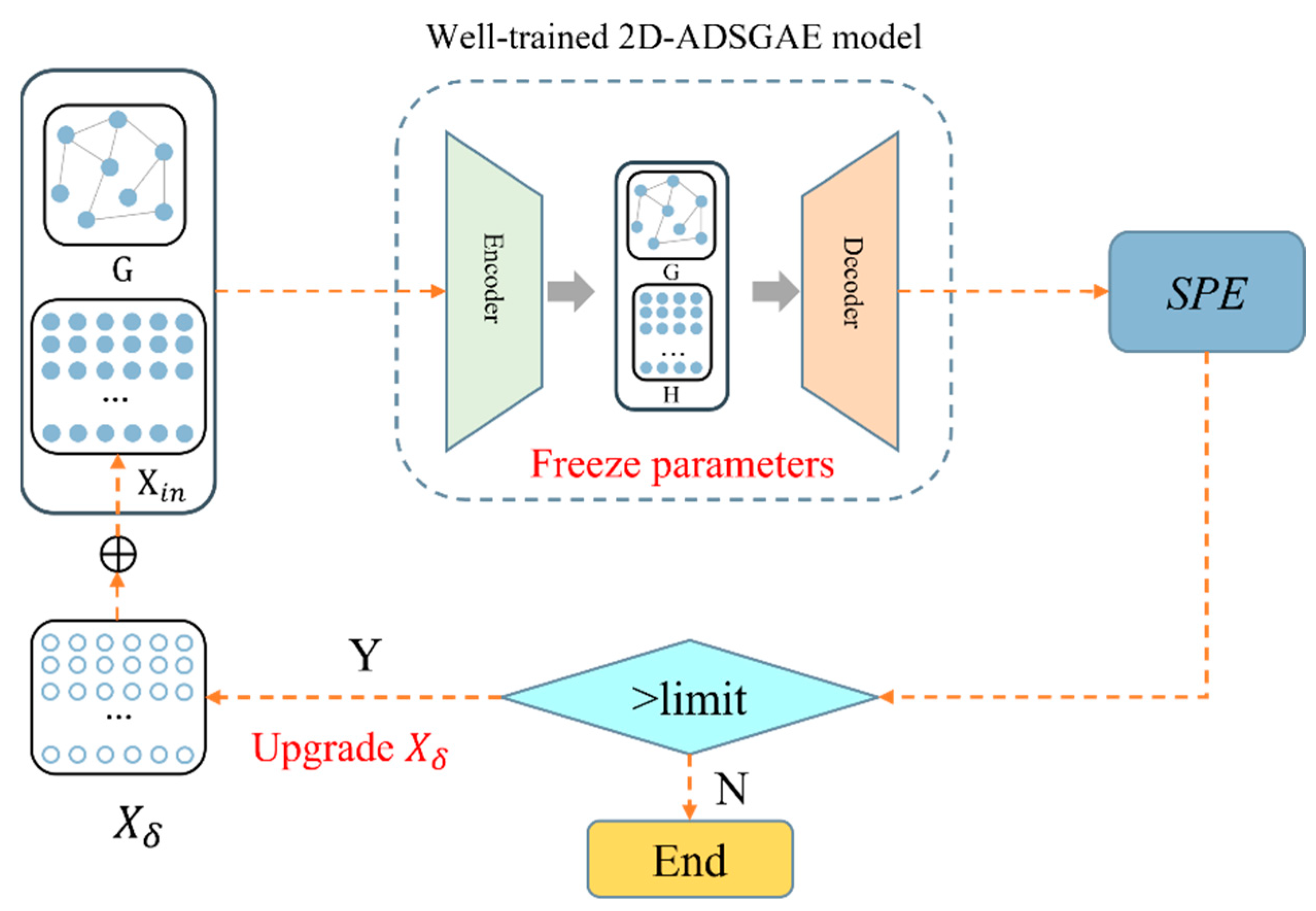
When a fault is detected, the model reports an alarm, but the alarm does not provide further information about the fault; so, a diagnosis of the fault is needed [29]. Inspired by Alcala’s research [30], this paper introduced a novel fault diagnosis method, named DRBC. Figure 6 shows the structure of DRBC. Assume that the variable of the sample is the fault variable. Let be the fault direction and be the fault magnitude. A value of 1 in the direction vector denotes a defective variable, while 0 denotes a normal variable. The goal is to combine and to reduce the SPE of below the control limit. Essentially, we need to optimize the incremental matrix step by step. During the iterative optimization process, the model parameters remain fixed, and is updated via backpropagation until the fault diagnosis concludes, indicated by the condition that the SPE falls below the corresponding control limit.
3.5. Monitoring Procedure
The flowchart of the offline modeling and online monitoring flow is shown in Figure 7. The offline modeling and online monitoring procedure is summarized as follows.
Offline modeling:
- Step 1:
- Normalize the training samples. Normalize the training data to zero mean and unit variance.
- Step 2:
- Divide the phases and determine the shape of the 2D sliding windows of each phase.
- Step 3:
- Construct the graph. Each sample is embedded into the graph as a node feature.
- Step 4:
- Train the 2D-ADSGAE model to obtain the optimal parameters.
- Step 5:
- Obtain the reconstructed data.
- Step 6:
- Calculate the SPE statistic for each sample by (13).
- Step 7:
- Compute the control limit of SPE by KDE.
Online monitoring:
- Step 1:
- Collect new samples and normalize using the parameters of the training set.
- Step 2:
- Judge phase and select the 2D sliding window.
- Step 3:
- Construct the graph.
- Step 4:
- Use the trained 2D-ADSGAE model to obtain the reconstructed data of .
- Step 5:
- Calculate the SPE of .
- Step 6:
- Alarm if SPE exceeds the control limit, and then turn to fault diagnosis. Otherwise, is normal.
The experiments were performed on a computer with the following specifications: CPU: Intel(R) Xeon(R) Silver 4210 CPU @ 2.20GHz manufactured in the United States by Intel Corporation, headquartered in Santa Clara, CA, USA; RAM: Samsung 128 GB produced by Samsung Electronics, with headquarters located in Seoul, Republic of Korea; GPU: NVIDIA Tesla V100 manufactured in Taiwan, China, by Delta Electronics; and Operating System: Ubuntu 18.04.6 LTS 64-bit.
4. Case Studies
In this section, we used two cases to demonstrate the validity of 2D-ADSGAE: one was the penicillin fermentation process and the other was the Lactobacillus plantarum replenishment fed-batch fermentation process. We also introduced three models, MPCA, variational autoencoder (VAE), and long short-term memory autoencoder (LSTM-AE), to compare to 2D-ADSGAE.
4.1. Penicillin Fermentation Process
The penicillin fermentation process, a classical batch process widely employed in process monitoring, is effectively simulated by the penicillin simulation platform (PenSim v2.0) [31], which offers a more realistic portrayal of numerical changes and can therefore verify the validity of 2D-ASGAE. In this paper, 10 variables in the penicillin fermentation process were selected for monitoring modeling, as shown in Table 1. Setting the reaction time of each batch as 600 h and the sampling interval as 0.5 h, a total of 1200 samples were collected in each batch. A total of 114 batches of data were generated, of which 80 batches were used as the training set, 20 batches were set as the validation set, and the remaining 14 batches were used as the fault test data. Table 2 provides a detailed description of the 14 fault types.
4.1.1. Parameter Setting
According to Algorithm 1, we divided the batch process into four phases: phase 1: 0-150, phase 2: 150-600, phase 3: 600-1100, and phase 4: 1100-1200. LSTM-AE uses the same period division scheme as 2D-ADSGAE and LSTM-AE employs a 1D sliding window with 10 samples in a window. The size of the 2D sliding windows of 2D-ADSGAE was determined via Algorithm 2. The 2D sliding window shape used by VAE is 10 × 6, where 10 is the time order and 6 is the batch order. The latent space dimension of the DPCA was finally determined to be 4 based on the contributions of the components. For fairness, the latent space dimensions of the VAE, LSTM-AE, and 2D-ADSGAE were also set to 4. The whole structure of the 2D-ADSGAE was set to be 10-6-4-6-10, and in the pre-training phase, the model learning rate was set to 0.002 for 800 iterations, while the parameters were optimized using the Adam optimizer [32]. In the fine-tuning stage, the model learning rate was set to 0.0005, and the number of iterations was set to 200. For fault diagnosis, the learning rate of the diagnostic model was set to 0.001, and the default value of the number of iterations was set to 1000. The number of iterations of the diagnostic model was adjusted according to the results of the diagnostic plot.
4.1.2. Fault Detection Results
In this part, we compared the fault detection performance of the proposed AGDAE on the penicillin fermentation process with MPCA, VAE, and LSTM-AE and calculated the fault detection rate (FDR) and false alarm rate (FAR) to evaluate the performance quantitatively. Table 3 shows the detection results of SPE statistics for different models on 14 faults.
Table 3 displays SPE statistics for four different models on 14 faults. Remarkably, 2D-ADSGAE excels with an impressive 93.57% average FDR, credited to its incorporation of two-dimensional dynamics and the effective filtering of redundant information within the sliding window. Notably, the conventional linear method, MPCA, proves ineffective in detecting faults of smaller magnitudes, such as 1, 4, 5, 8, 9, and 10. However, neural network-based nonlinear methods, like VAE, LSTM-AE, and 2D-ADSGAE, exhibit enhanced capability in extracting nonlinear features from penicillin data, resulting in significantly higher average fault detection rates compared to MPCA.
LSTM-AE, utilizing sliding windows in the batch direction, effectively captures dynamic batch process data characteristics, resulting in a higher average fault detection rate compared to VAE. Nevertheless, its exclusive emphasis on batch direction dynamics alone leads to an inferior detection performance compared to that of 2D-ADSGAE. In contrast, 2D-ADSGAE employs a graph structure to handle batch process data. It determines sample node neighborhood information through 2D nonlinear dynamics in both the batch and time directions. By employing the Euclidean distance, correlation, and SoftMax function, it determines edge weights between adjacent nodes in the graph, effectively capturing dynamics. Additionally, the self-attention mechanism dynamically allocates attention weights to each node based on the features of neighboring nodes, reducing the interference of redundant information on the model. This adaptive learning of node relationships allows 2D-ADSGAE to capture crucial node distinctions. The results underscore the superior exploitation of dynamic information within batch process data by 2D-ADSGAE.
Figure 8 and Figure 9 present detailed detection outcomes for faults 1 and 4, respectively. In these detection plots, the blue dots depict the initial 400 normal samples, the red dots represent the subsequent 800 fault samples, and the black dotted line signifies the control limit.
Figure 8 shows the four detection plots for fault 1. From the figure, we can see that MPCA cannot detect fault 1. Although the SPE values of the fault samples produce fluctuations, they are still below the control limit. While the FDRs of VAE, LSTM-AE, and 2D-ADSGAE are 96.46%, 96.63%, and 97.80%, respectively, these three methods achieve satisfactory detection results. From this, we can see that linear methods may not be suitable for multivariate nonlinear processes. In contrast, VAE, LSTM-AE, and 2D-ADSGAE are nonlinear methods based on neural networks, which are more suitable for dealing with batch process data.
Figure 9 displays the detection outcomes for fault 4. The plot indicates that 2D-ADSGAE distinctly identifies the slight fault and effectively segregates the fault samples from the normal ones. Referring to Table 3, the FDRs for MPCA, VAE, and LSTM-AE are 0.00%, 20.48%, and 45.38%, respectively, none of which surpasses 50%. This underscores the inability of these three methods to accurately detect fault 4. In contrast, 2D-ADSGAE achieves an impressive fault detection rate of 97.25%, surpassing the performance of the other three detection methods. This indicates 2D-ADSGAE adeptly learns the underlying dynamic properties using the self-attention mechanism, facilitating the easy detection of such faults. In contrast, LSTM-AE simply splices the data in the sliding window and ascribes the same weight to each sample, which does not fully learn the dynamic information in the batch process data. Therefore, fully capturing the dynamic characteristics in the data is the focus of fault detection. Experiments have shown that graph structures and self-attention mechanisms are more suitable and process dynamic information than the simple splicing of the samples.
4.1.3. Fault Diagnosis Results
Since we detected the faults in Section 4.1.2, this subsection used DRBC to diagnose the faults. Firstly, the ground truths for faults 3, 10, and 14 are shown in Figure 10 Detailed information about the variables can be obtained from Table 1. The larger values in the graph represent the larger magnitude of the fault, and the blue bar represents the duration of the fault. From the plot, we know that faults 3 and 10 are univariate faults, while fault 14 is a multivariate fault.
Figure 10a–c present the diagnosis plots of fault 3 with 2000 iterations, fault 10 with 2000 iterations, and fault 14 with 1000 iterations, respectively. Upon analyzing the diagnosis results of fault 3, it is apparent that an abnormality in variable 2 initiates the fault at moment 400, persisting until moment 1200. From Table 1 and Table 2, it can be seen that fault 3 is the result of a 5% increase in the agitator power, starting at the 400 moment and ending at the 1200 moment.
The diagnostic findings pertaining to fault 10 indicate a fault state within variable 1, initiating at approximately moment 400 and persisting until moment 1200. Concurrently, the established ground truth for fault 10 denotes a 3% increase in the aeration rate, commencing at moment 400 and extending until moment 1200. Moreover, the diagnostic outcomes for fault 14 reveal a multivariate fault attributed to the combined faults within variables 2, 4, and 9, manifesting from moment 600 and continuing until moment 1000. It is discerned from Table 2 that fault 14 indeed arises from faults observed in three distinct variables: the agitator power, pH, and feed temperature. It is noteworthy that the ground truth representation for fault 14 exhibits lighter color variations in variables 2 and 9. Nevertheless, the diagnostic result plot distinctly portrays faults within these specific variables. This serves to highlight the efficacy of the fault diagnosis method grounded on the depth contribution graph, showcasing its capability to accurately localize and analyze faults within the system.
4.2. Lactobacillus Plantarum Fed-Batch Fermentation Process
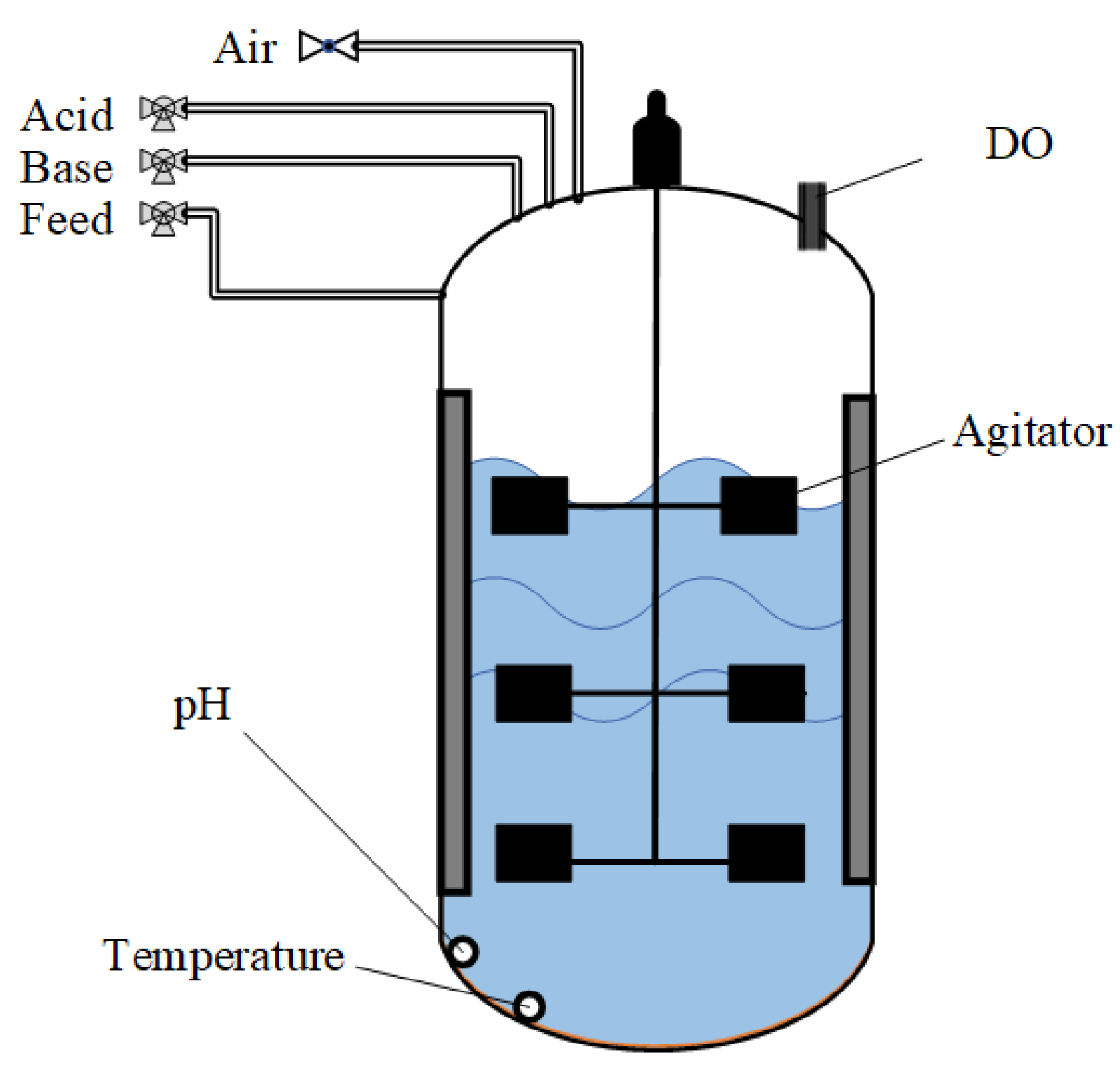
Lactobacillus plantarum, as a multifunctional bacterium, has a wide range of applications in the food industry, nutraceuticals, and medical fields [33,34]. The Lactobacillus plantarum fed-batch fermentation process is a classical batch process, showcasing its fermentation equipment in Figure 11. This study focused on seven variables within the Lactobacillus plantarum fermentation process, as outlined in Table 4, specifically selected for monitoring and modeling purposes. Each batch within this process maintains an 8 h reaction time, coupled with a sampling interval of 1 min, thereby enabling the collection of a total of 480 samples per batch. The dataset comprises a total of 25 batches, with 20 batches allocated for training, 2 batches designated for validation, and the remaining 3 batches assigned for failure test data. Table 5 offers an intricate description of the three fault types encountered in this study.
4.2.1. Parameter Setting
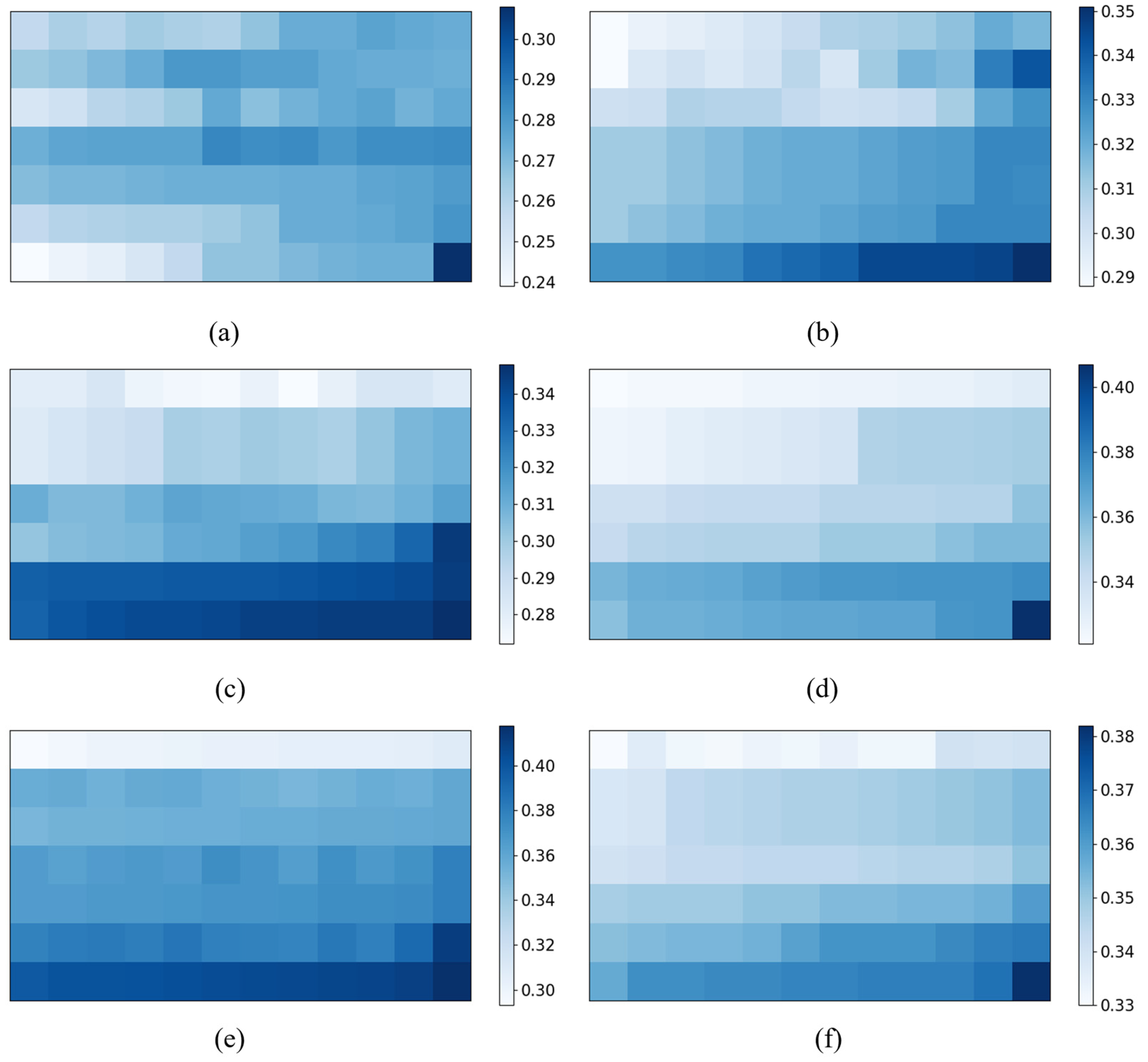
In this section, MPCA, VAE, and LSTM-AE were used as comparison experiments for 2D-ADSGAE. The latent space dimension was set to 3 for all models, and the structure of 2D-ADSGAE was set to 7-7-3-7-7. In the pre-training phase, the model learning rate was set to 0.002 and the number of iterations was set to 800, while the Adam optimizer was used to optimize the parameters. In the fine-tuning phase, the model learning rate was set to 0.0005 and the number of iterations was set to 200. For fault diagnosis, the learning rate of the diagnostic model was set to 0.001 and the default value of the number of iterations was 1000. According to Algorithm 1, we divided the process into six phases, phase 1: 0–60, phase 2: 60–160, phase 3: 160–240, phase 4: 240–320, phase 5: 320–400, and phase 6: 400–480.
Figure 12 demonstrates the sample correlation in the sliding windows on the different phases of the Lactobacillus plantarum fed-batch fermentation process. The figure illustrates the varying 2D dynamic characteristics across the different phases, indicating that the composition of 2D sliding windows varies within each phase. Meanwhile, it is notable that the majority of the sliding windows exhibit irregular shapes.
4.2.2. Fault Detection Results
Table 6 shows the detection results of SPE statistics for MPCA, VAE, LSTM-AE, and 2D-ADSGAE on three faults. From the table, it can be noticed that 2D-ADSGAE has the highest average fault detection rate of 96.67%, which once again proves 2D-ADSGAE’s ability to extract dynamic information. Notice that, although the average fault detection rate of LSTM-AE is very close to that of VAE, the average FAR of VAE is indeed the highest among all models, which indicates that VAE is not yet able to adequately mine the potential dynamic information of the batch process data.
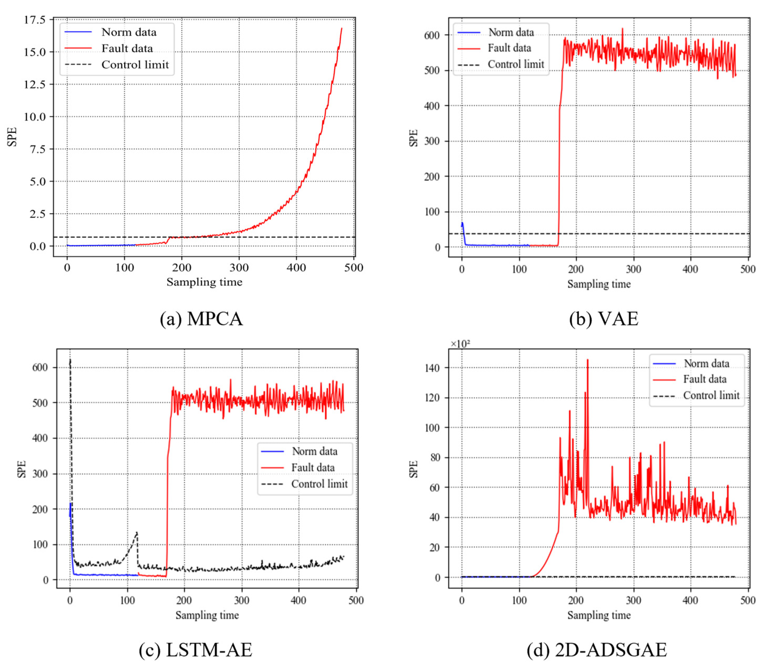
Figure 13 provides a detailed representation of the four detection outcomes for fault 3. Notably, in Figure 13d, 2D-ADSGAE detects the fault in its early stages of occurrence. The detection curve depicted in the figure exhibits a gradual increase until the fault magnitude escalates significantly. Conversely, VAE and LSTM-AE begin to detect fault information abruptly, commencing at around the 170th sampling time. These experimental findings highlight that 2D-ADSGAE adeptly captures the dynamic information of process data, gradually accumulating fault information during the early stages and thereby enhancing the fault detection rate.
4.2.3. Fault Diagnosis Results
After the fault detection, this section carried out the fault diagnosis, and the ground truths of the three faults are shown in Figure 14. From the figure, we can see that the diagnosis results for all three faults are clear. For fault 3, it can be seen that the proposed DRBC fault diagnosis algorithm is effective for multivariate faults in Lactobacillus plantarum fed-batch fermentation processes.
5. Conclusions
In this paper, a new 2D-ADSGAE model was proposed to extract nonlinearity and dynamics in batch processes. A method based on sample correlations within sliding windows was introduced for phase division. Through this method, we further determined the shape of the 2D sliding window within each phase, thereby establishing neighborhood information for nodes in the graph. The attention mechanism was employed to handle redundant information and nonlinear dynamics among samples within the sliding window. Additionally, a monitoring metric was established within the residual space. Finally, it was combined with DRBC for fault variable localization and analysis. The results of the two experiments demonstrate that 2D-ADSGAE outperforms the other models, significantly enhancing the fault detection accuracy and enabling the analysis and localization of fault variables.
Note that the proposed model does not distinguish between quality-related and non-quality-related faults, and this will be considered in our future work to further improve the monitoring capability of the model.
Author Contributions
J.Z.: methodology, supervision, and writing—review and editing. X.G.: data curation, methodology, investigation, and writing—review and editing. Z.Z.: supervision, conceptualization, methodology, and writing—review and editing. All authors have read and agreed to the published version of the manuscript.
Funding
This research was funded by the Natural Science Foundation of Jiangsu Province (Grant No. BK20210452), the National Natural Science Foundation of China (Grant No. 62103168), and the Fundamental Research Funds for the Central Universities (JUSRP622034).
Data Availability Statement
The data presented in this study are available upon request from the corresponding author.
Conflicts of Interest
The authors declare no conflicts of interest.
References
- Gao, K.; Lu, J.; Xu, Z.; Gao, F. Control-Oriented Two-Dimensional Online System Identification for Batch Processes. Ind. Eng. Chem. Res. 2021, 60, 7656–7666. [Google Scholar] [CrossRef]
- Zhang, Z.; Zhu, J.; Ge, Z. Industrial process modeling and fault detection with recurrent Kalman variational autoencoder. In Proceedings of the 2020 IEEE 9th Data Driven Control and Learning Systems Conference (DDCLS), Liuzhou, China, 19–21 June 2020; IEEE: Piscataway, NJ, USA, 2020; pp. 1370–1376. [Google Scholar]
- Peng, K.; Ma, L.; Zhang, K. Review of quality-related fault detection and diagnosis techniques for complex industrial processes. Acta Autom. Sin. 2017, 43, 349–365. [Google Scholar]
- Jiang, Q.; Gao, F.; Yan, X.; Yi, H. Multiobjective two-dimensional CCA-based monitoring for successive batch processes with industrial injection molding application. IEEE Trans. Ind. Electron. 2018, 66, 3825–3834. [Google Scholar] [CrossRef]
- Qin, S.J. Survey on data-driven industrial process monitoring and diagnosis. Annu. Rev. Control 2012, 36, 220–234. [Google Scholar] [CrossRef]
- Yin, S.; Ding, S.X.; Xie, X.; Luo, H. A review on basic data-driven approaches for industrial process monitoring. IEEE Trans. Ind. Electron. 2014, 61, 6418–6428. [Google Scholar] [CrossRef]
- Jiang, Q.; Yan, X.; Huang, B. Deep discriminative representation learning for nonlinear process fault detection. IEEE Trans. Autom. Sci. Eng. 2019, 17, 1410–1419. [Google Scholar] [CrossRef]
- Ammiche, M.; Kouadri, A.; Bakdi, A. A combined monitoring scheme with fuzzy logic filter for plant-wide Tennessee Eastman Process fault detection. Chem. Eng. Sci. 2018, 187, 269–279. [Google Scholar] [CrossRef]
- Nomikos, P.; MacGregor, J.F. Monitoring batch processes using multiway principal component analysis. AlChE J. 1994, 40, 1361–1375. [Google Scholar] [CrossRef]
- Nomikos, P.; MacGregor, J.F. Multi-way partial least squares in monitoring batch processes. Chemom. Intell. Lab. Syst. 1995, 30, 97–108. [Google Scholar] [CrossRef]
- Zhang, S.; Zhao, C. Slow-feature-analysis-based batch process monitoring with comprehensive interpretation of operation condition deviation and dynamic anomaly. IEEE Trans. Ind. Electron. 2018, 66, 3773–3783. [Google Scholar] [CrossRef]
- Peng, C.; Zhang, R.Y.; Ding, C.H. Dynamic hidden variable fuzzy broad neural network based batch process anomaly detection with incremental learning capabilities. Expert Syst. Appl. 2022, 202, 117390. [Google Scholar] [CrossRef]
- Zhang, Q.; Li, P.; Lang, X.; Miao, A. Improved dynamic kernel principal component analysis for fault detection. Measurement 2020, 158, 107738. [Google Scholar] [CrossRef]
- Bounoua, W.; Bakdi, A. Fault detection and diagnosis of nonlinear dynamical processes through correlation dimension and fractal analysis based dynamic kernel PCA. Chem. Eng. Sci. 2021, 229, 116099. [Google Scholar] [CrossRef]
- Chen, J.; Liu, K.-C. On-line batch process monitoring using dynamic PCA and dynamic PLS models. Chem. Eng. Sci. 2002, 57, 63–75. [Google Scholar] [CrossRef]
- Lu, N.; Yao, Y.; Gao, F.; Wang, F. Two-dimensional dynamic PCA for batch process monitoring. AlChE J. 2005, 51, 3300–3304. [Google Scholar] [CrossRef]
- Yao, Y.; Chen, T.; Gao, F. Multivariate statistical monitoring of two-dimensional dynamic batch processes utilizing non-Gaussian information. J. Process Control 2010, 20, 1188–1197. [Google Scholar] [CrossRef]
- Jiang, Q.; Yan, S.; Yan, X.; Yi, H.; Gao, F. Data-driven two-dimensional deep correlated representation learning for nonlinear batch process monitoring. IEEE Trans. Ind. Inf. 2019, 16, 2839–2848. [Google Scholar] [CrossRef]
- Ren, J.; Ni, D. A batch-wise LSTM-encoder decoder network for batch process monitoring. Chem. Eng. Res. Des. 2020, 164, 102–112. [Google Scholar] [CrossRef]
- Andrus, B.R.; Nasiri, Y.; Cui, S.; Cullen, B.; Fulda, N. Enhanced story comprehension for large language models through dynamic document-based knowledge graphs. In Proceedings of the AAAI Conference on Artificial Intelligence, Vancouver, BC, Canada, 20–27 February 2022; pp. 10436–10444. [Google Scholar]
- Ding, Y.; Zhang, Z.; Zhao, X.; Hong, D.; Cai, W.; Yang, N.; Wang, B. Multi-scale receptive fields: Graph attention neural network for hyperspectral image classification. Expert Syst. Appl. 2023, 223, 119858. [Google Scholar] [CrossRef]
- Ding, C.; Sun, S.; Zhao, J. MST-GAT: A multimodal spatial–temporal graph attention network for time series anomaly detection. Inf. Fusion 2023, 89, 527–536. [Google Scholar] [CrossRef]
- Li, Z.L.; Zhang, G.W.; Yu, J.; Xu, L.Y. Dynamic graph structure learning for multivariate time series forecasting. Pattern Recognit. 2023, 138, 109423. [Google Scholar] [CrossRef]
- Zhang, Y.; Yu, J. Pruning graph convolutional network-based feature learning for fault diagnosis of industrial processes. J. Process Control 2022, 113, 101–113. [Google Scholar] [CrossRef]
- Liu, L.; Zhao, H.; Hu, Z. Graph dynamic autoencoder for fault detection. Chem. Eng. Sci. 2022, 254, 117637. [Google Scholar] [CrossRef]
- Veličković, P.; Cucurull, G.; Casanova, A.; Romero, A.; Lio, P.; Bengio, Y. Graph attention networks. arXiv 2017, arXiv:1710.10903. [Google Scholar]
- Zhang, S.; Bao, X. Two-dimensional multiphase batch process monitoring based on sparse canonical variate analysis. J. Process Control 2022, 116, 185–198. [Google Scholar] [CrossRef]
- Samuel, R.T.; Cao, Y. Nonlinear process fault detection and identification using kernel PCA and kernel density estimation. Syst. Sci. Control Eng. 2016, 4, 165–174. [Google Scholar] [CrossRef]
- Zhang, Z.; Zhu, J.; Zhang, S.; Gao, F. Process monitoring using recurrent Kalman variational auto-encoder for general complex dynamic processes. Eng. Appl. Artif. Intell. 2023, 123, 106424. [Google Scholar] [CrossRef]
- Alcala, C.F.; Qin, S.J. Reconstruction-based contribution for process monitoring. Automatica 2009, 45, 1593–1600. [Google Scholar] [CrossRef]
- Birol, G.; Ündey, C.; CInar, A. A modular simulation package for fed-batch fermentation: Penicillin production. Comput. Chem. Eng. 2002, 26, 1553–1565. [Google Scholar] [CrossRef]
- Kingma, D.P.; Ba, J. Adam: A method for stochastic optimization. arXiv 2014, arXiv:1412.6980. [Google Scholar]
- Seddik, H.A.; Bendali, F.; Gancel, F.; Fliss, I.; Spano, G.; Drider, D. Lactobacillus plantarum and its probiotic and food potentialities. Probiotics Antimicrob. Proteins 2017, 9, 111–122. [Google Scholar] [CrossRef] [PubMed]
- Krieger-Weber, S.; Heras, J.M.; Suarez, C. Lactobacillus plantarum, a new biological tool to control malolactic fermentation: A review and an outlook. Beverages 2020, 6, 23. [Google Scholar] [CrossRef]
Figure 1.
(a) Structure of AE. (b) Overview of SAE.

Figure 2.
Phase division and the sliding windows in different phases.

Figure 3.
Two-dimensional sliding window in batch process data.

Figure 4.
Sample correlation in the sliding windows at different phases of the penicillin fermentation process. We divide the penicillin fermentation process into four phases. (a–d) represent the sample correlation of the sliding windows in four phases.
Figure 4.
Sample correlation in the sliding windows at different phases of the penicillin fermentation process. We divide the penicillin fermentation process into four phases. (a–d) represent the sample correlation of the sliding windows in four phases.


Figure 5.
The overview of 2D-ADSGAE.

Figure 6.
The structure of the fault diagnosis.

Figure 7.
Flowchart of 2D-ADSGAE for process monitoring.

Figure 8.
Monitoring charts of fault 1 with 4 different methods.

Figure 9.
Monitoring charts of fault 4 with 4 different methods.

Figure 10.
Diagnosis plots and ground truths for faults 3, 10, and 14.

Figure 11.
The overall structure of the Lactobacillus plantarum fermentation process.

Figure 12.
Sample correlation in the sliding windows at the different phases of the Lactobacillus plantarum fed-batch fermentation process. We divide the penicillin fermentation process into six phases. (a–f) represent the sample correlation of the sliding windows in six phases.
Figure 12.
Sample correlation in the sliding windows at the different phases of the Lactobacillus plantarum fed-batch fermentation process. We divide the penicillin fermentation process into six phases. (a–f) represent the sample correlation of the sliding windows in six phases.

Figure 13.
Monitoring results of fault 3 with 4 different methods.

Figure 14.
Diagnosis plots and ground truths for faults 1, 2, and 3.


Table 1.
Process variables used in the case study.
| No. | Variable | Normal Value |
|---|---|---|
| 1 | Aeration rate (L/h) | 8.6 |
| 2 | Agitator power (W) | 30 |
| 3 | Substrate feed rate (L/h) | 0.042 |
| 4 | Feed temperature (K) | 296 |
| 5 | DO conc. (mmole/L) | 1.16 |
| 6 | Biomass conc. (g/L) | 0.1 |
| 7 | Penicillin conc. (g/L) | 0 |
| 8 | CO2 conc. (mmole/L) | 0.5 |
| 9 | pH | 5 |
| 10 | Temperature (K) | 298 |
Table 2.
Fault types during the penicillin fermentation process.
| Fault No. | Variable | Type | Description | Start | End |
|---|---|---|---|---|---|
| 1 | Agitator power | Step | +2% | 400 | 1200 |
| 2 | Agitator power | Step | +3% | 400 | 1200 |
| 3 | Agitator power | Step | +5% | 400 | 1200 |
| 4 | pH | Step | −3% | 400 | 1200 |
| 5 | pH | Step | −5% | 400 | 1200 |
| 6 | Substrate feed rate | Ramp | +0.01L/h | 400 | 1200 |
| 7 | Substrate feed rate | Ramp | −0.015L/h | 400 | 1200 |
| 8 | Aeration rate | Step | −1% | 400 | 1200 |
| 9 | Aeration rate | Step | +2% | 400 | 1200 |
| 10 | Aeration rate | Step | +3% | 400 | 1200 |
| 11 | Aeration rate | Ramp | +0.05L/h | 600 | 1000 |
| 12 | Aeration rate | Ramp | −0.05L/h | 600 | 1000 |
| 13 | Agitator power/pH/Substrate feed temperature | Step | +5%/+5%/+3% | 600 | 1000 |
| 14 | Agitator power/pH/Substrate feed temperature | Step | +5%/−5%/−3% | 600 | 1000 |
Table 3.
False alarm rate (%) and fault detection rate (%) of MPCA, VAE, LSTM-AE, and 2D-ADSGAE in the penicillin fermentation process. The optimal performance of FDR has been emphasized in bold within the table.
Table 3.
False alarm rate (%) and fault detection rate (%) of MPCA, VAE, LSTM-AE, and 2D-ADSGAE in the penicillin fermentation process. The optimal performance of FDR has been emphasized in bold within the table.
| Fault No. | MPCA | VAE | LSTM-AE | 2D-ADSGAE | ||||
|---|---|---|---|---|---|---|---|---|
| FAR | FDR | FAR | FDR | FAR | FDR | FAR | FDR | |
| 1. | 3.25 | 0.00 | 0.25 | 96.46 | 0.00 | 96.63 | 0.00 | 97.80 |
| 2 | 3.25 | 64.13 | 1.00 | 100.00 | 0.00 | 99.63 | 0.50 | 100.00 |
| 3 | 3.50 | 100.00 | 1.50 | 100.00 | 0.25 | 100.00 | 0.50 | 100.00 |
| 4 | 3.25 | 0.00 | 0.50 | 20.48 | 0.00 | 45.38 | 0.00 | 97.25 |
| 5 | 3.25 | 0.00 | 0.25 | 90.90 | 0.00 | 93.75 | 0.00 | 98.25 |
| 6 | 3.25 | 35.90 | 0.50 | 56.88 | 0.00 | 63.86 | 0.00 | 73.13 |
| 7 | 3.25 | 60.62 | 0.25 | 48.29 | 0.00 | 57.50 | 0.00 | 71.25 |
| 8 | 3.25 | 0.00 | 0.50 | 68.90 | 0.25 | 90.25 | 0.25 | 97.75 |
| 9 | 3.25 | 0.00 | 0.75 | 100.00 | 0.25 | 100.00 | 0.25 | 100.00 |
| 10 | 3.25 | 0.00 | 0.50 | 100.00 | 0.25 | 100.00 | 0.25 | 100.00 |
| 11 | 3.25 | 0.00 | 0.00 | 80.66 | 0.00 | 83.13 | 0.00 | 93.75 |
| 12 | 3.25 | 0.00 | 0.50 | 71.30 | 0.00 | 73.63 | 0.00 | 80.75 |
| 13 | 2.38 | 99.25 | 1.40 | 100.00 | 0.00 | 100.00 | 0.45 | 100.00 |
| 14 | 2.00 | 100.00 | 1.30 | 100.00 | 0.00 | 100.00 | 0.45 | 100.00 |
| Average | 3.12 | 32.85 | 0.66 | 80.99 | 0.07 | 85.98 | 0.19 | 93.57 |
Table 4.
Process variables used in case study 2.
| No. | Variable | Normal Value |
|---|---|---|
| 1 | Temperature (K) | 310 |
| 2 | pH | 6 |
| 3 | DO conc. (mmole/L) | 98 |
| 4 | Agitator power (W) | 30 |
| 5 | Acid (mL/h) | 10 |
| 6 | Base (mL/h) | 30 |
| 7 | Substrate feed rate (mL/h) | 30 |
Table 5.
Fault types during the Lactobacillus plantarum fed-batch fermentation process.
| Fault No. | Variable | Type | Description | Start | End |
|---|---|---|---|---|---|
| 1 | pH | Step | +0.5 | 120 | 480 |
| 2 | Temperature | Step | +1% | 120 | 480 |
| 3 | pH/ Temperature | Step | +0.5/+1% | 120 | 480 |
Table 6.
False alarm rate (%) and fault detection rate (%) of VAE, LSTM-AE, and 2D-ADSGAE in the Lactobacillus plantarum fed-batch fermentation process. The optimal performance of FDR has been emphasized in bold within the table.
Table 6.
False alarm rate (%) and fault detection rate (%) of VAE, LSTM-AE, and 2D-ADSGAE in the Lactobacillus plantarum fed-batch fermentation process. The optimal performance of FDR has been emphasized in bold within the table.
| Fault No. | MPCA | VAE | LSTM-AE | 2D-ADSGAE | ||||
|---|---|---|---|---|---|---|---|---|
| FAR | FDR | FAR | FDR | FAR | FDR | FAR | FDR | |
| 1 | 0.00 | 76.11 | 4.17 | 90.00 | 0.00 | 90.00 | 0.00 | 90.28 |
| 2 | 0.00 | 99.44 | 0.00 | 99.72 | 0.00 | 99.44 | 0.25 | 100.00 |
| 3 | 0.00 | 74.40 | 3.33 | 86.11 | 0.00 | 86.11 | 0.83 | 99.72 |
| Average | 0.00 | 83.32 | 2.50 | 91.94 | 0.00 | 91.85 | 0.36 | 96.67 |
Disclaimer/Publisher’s Note: The statements, opinions and data contained in all publications are solely those of the individual author(s) and contributor(s) and not of MDPI and/or the editor(s). MDPI and/or the editor(s) disclaim responsibility for any injury to people or property resulting from any ideas, methods, instructions or products referred to in the content. |
© 2024 by the authors. Licensee MDPI, Basel, Switzerland. This article is an open access article distributed under the terms and conditions of the Creative Commons Attribution (CC BY) license (https://creativecommons.org/licenses/by/4.0/).
Share and Cite
MDPI and ACS Style
Zhu, J.; Gao, X.; Zhang, Z. Attention-Based Two-Dimensional Dynamic-Scale Graph Autoencoder for Batch Process Monitoring. Processes 2024, 12, 513. https://doi.org/10.3390/pr12030513
AMA Style
Zhu J, Gao X, Zhang Z. Attention-Based Two-Dimensional Dynamic-Scale Graph Autoencoder for Batch Process Monitoring. Processes. 2024; 12(3):513. https://doi.org/10.3390/pr12030513
Chicago/Turabian StyleZhu, Jinlin, Xingke Gao, and Zheng Zhang. 2024. "Attention-Based Two-Dimensional Dynamic-Scale Graph Autoencoder for Batch Process Monitoring" Processes 12, no. 3: 513. https://doi.org/10.3390/pr12030513
Note that from the first issue of 2016, this journal uses article numbers instead of page numbers. See further details here.