
A New Method for Numerical Simulation of Coalbed Methane Pilot Horizontal Wells—Taking the Bowen Basin C Pilot Area in Australia as an Example
 ,
,
Abstract
:1. Introduction
2. Pilot Well Overview
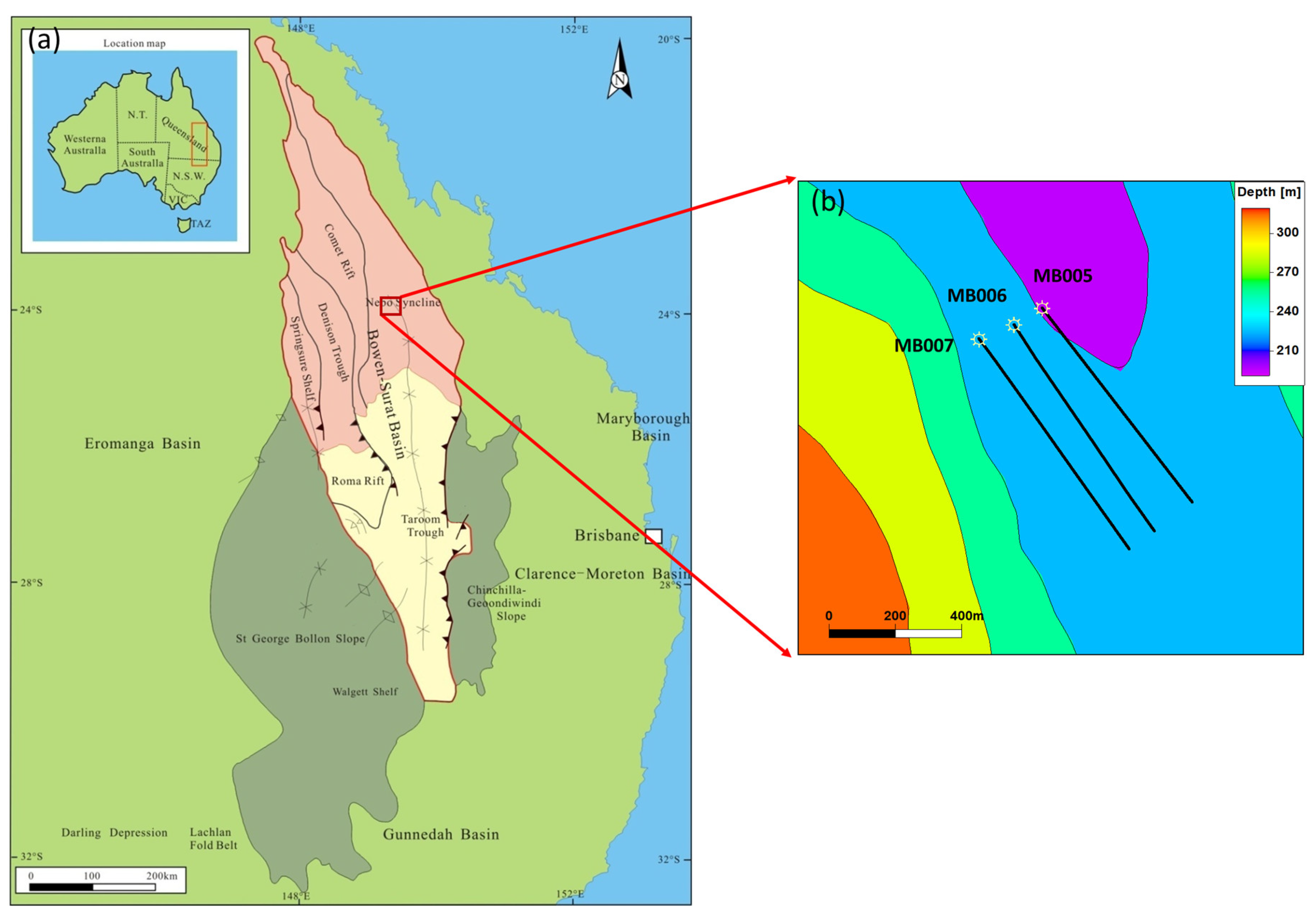
2.1. Geological Background
2.2. Characteristics of CBM Reservoirs
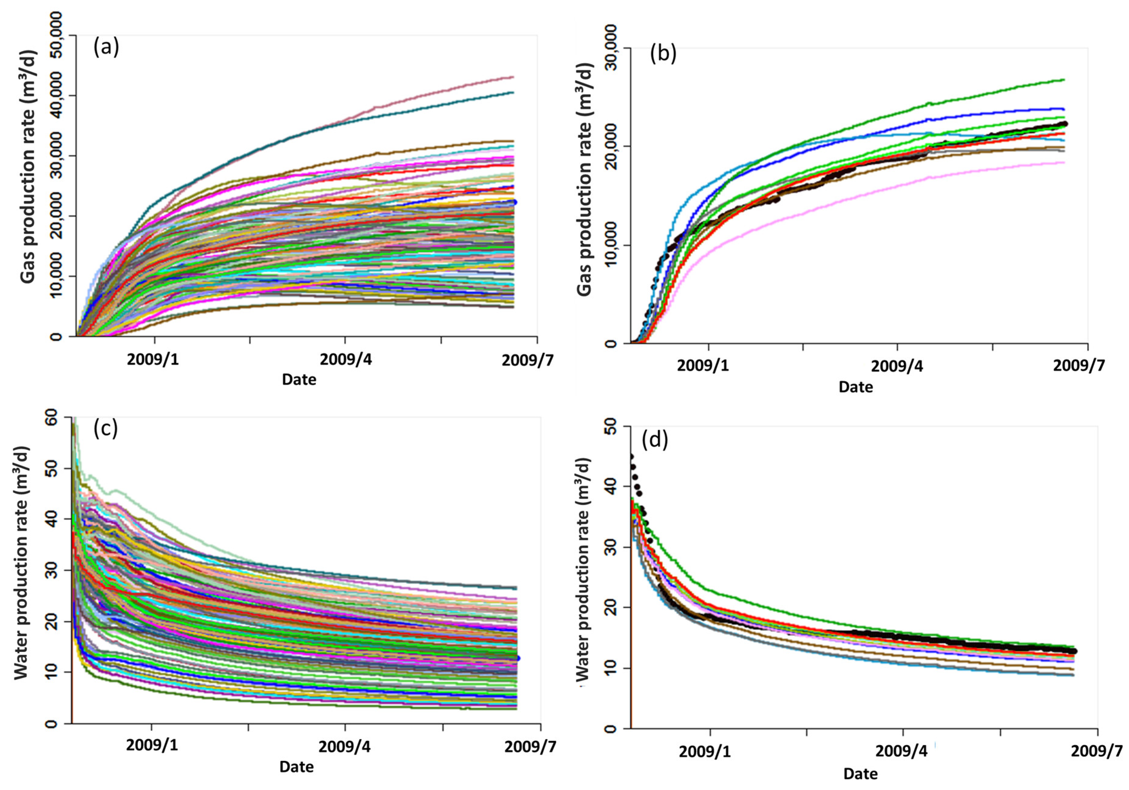
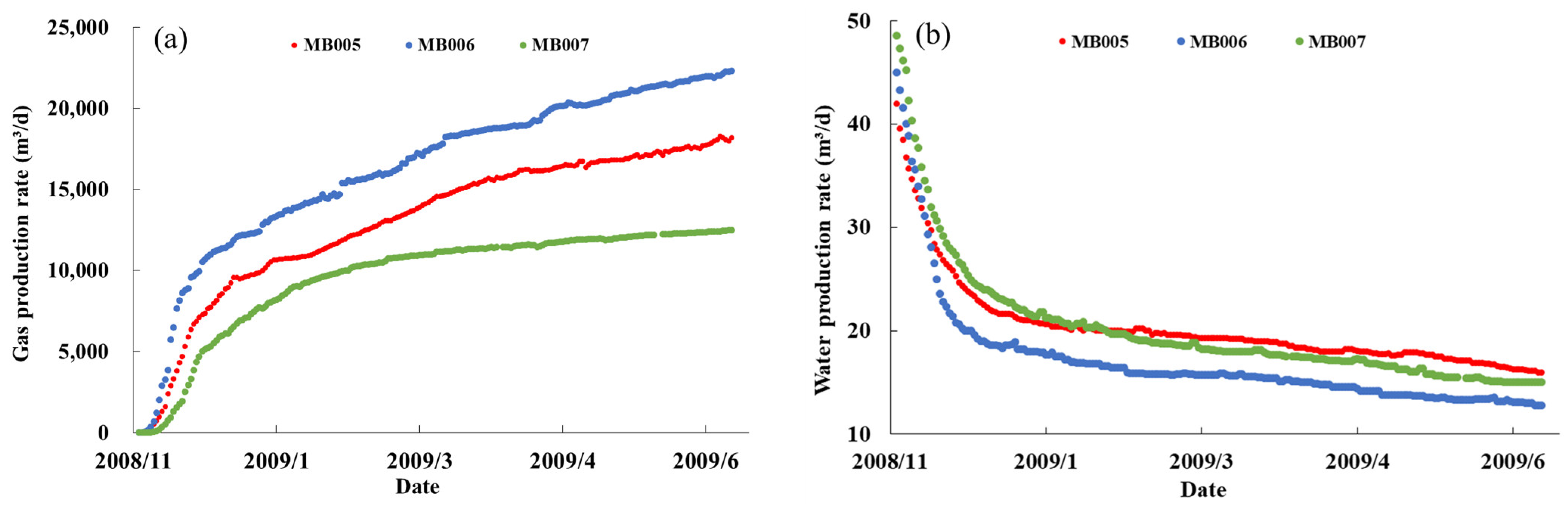
2.3. Production Characteristics of Pilot Wells
3. Numerical Simulation Workflow
4. Preparation before Numerical Simulation
4.1. Dynamic Model Initialization
4.2. Parameter Uncertainty Analysis
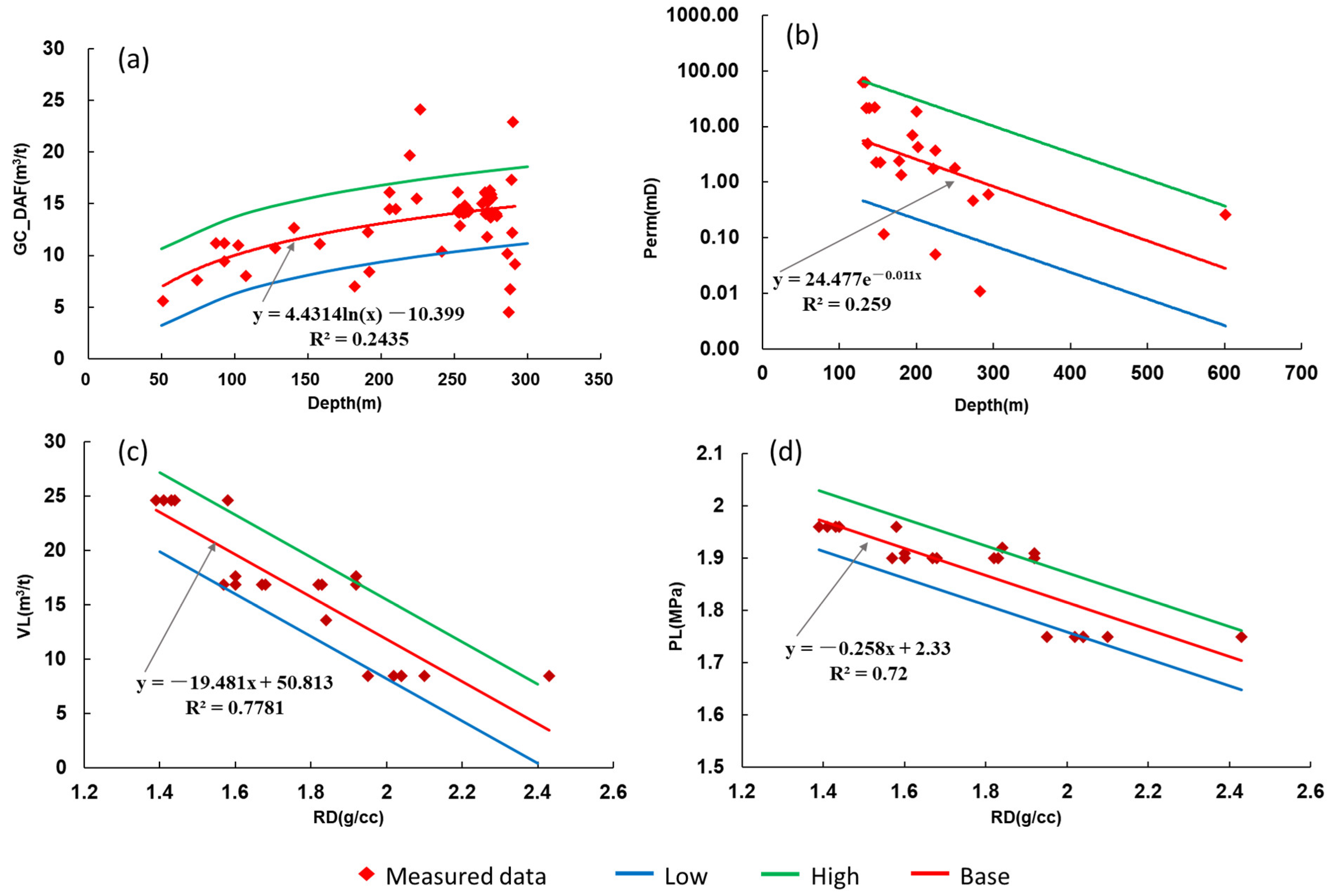
4.2.1. Analysis of Uncertainty in Trend Parameters
4.2.2. Analysis of Uncertainty in Non-Trend Parameters
4.3. Parameter Sensitivity Analysis
5. Numerical Simulation Process
5.1. Simulation Cases Generation and Analysis
5.2. Optimal Simulation Selection and EUR Prediction Method
6. Results and Discussion
6.1. EUR Prediction Results
6.2. Discussion
6.2.1. Application of Simulation Algorithms and Parameter Optimization
- (1)
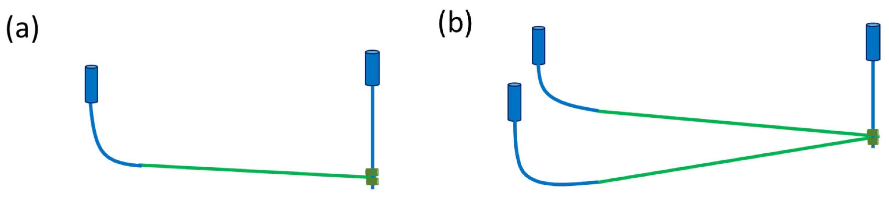
- Inscribed type
- (2)
- Face-centered type
6.2.2. Analysis of Differences in Parameter Sensitivity
6.2.3. Impact of Drilling Rate of Coal Seams on Gas Production
6.2.4. Comparison of EUR
7. Conclusions
- (1)
- The distribution of gas content, permeability, VL, and PL exhibits a pattern that can be predicted by establishing their correlations with other parameters, respectively. In contrast, the distribution of fracture porosity, gas relative permeability, water relative permeability, rock compressibility, and sorption time does not show a discernible pattern.
- (2)
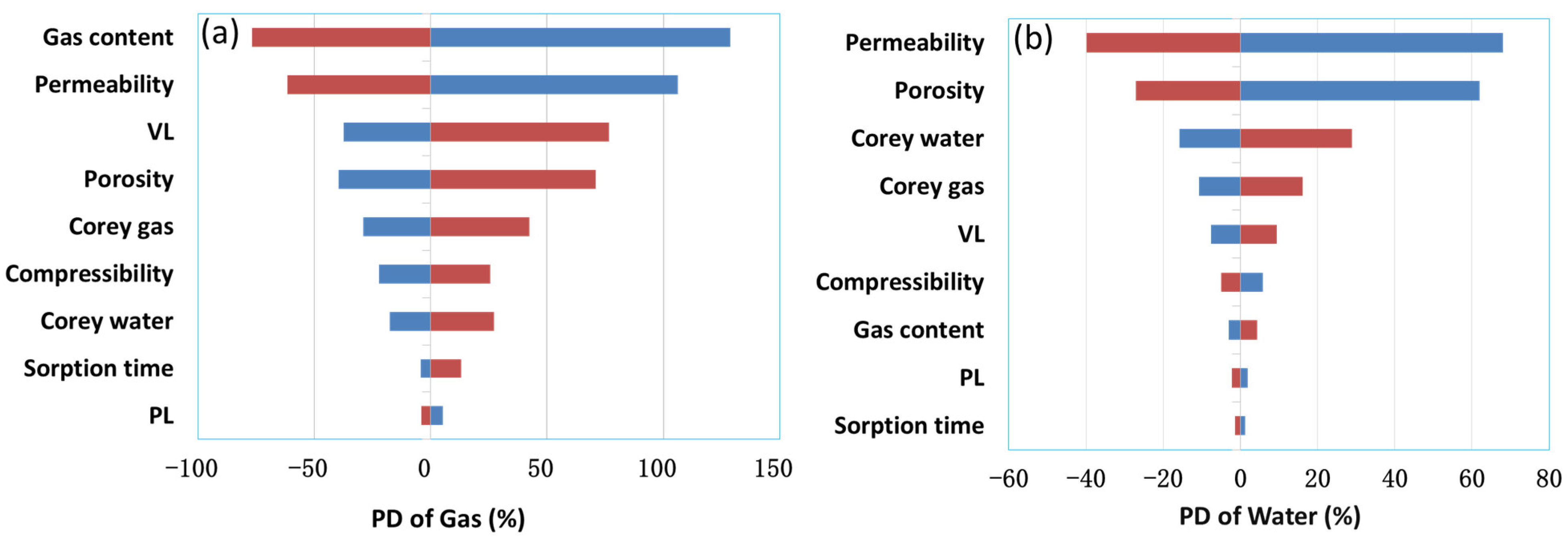
- The gas production is most sensitive to gas content and permeability, and the water production is most sensitive to fracture porosity and permeability. So, the uncertainty range settings of these four parameters are pivotal for the simulated EUR.
- (3)
- The ED method is an efficacious tool for analyzing parameter uncertainty, facilitating rapid history matching of production data, and identifying various combinations of CBM reservoir parameters, significantly reducing the time required for numerical simulation.
- (4)
- A higher drilling rate of the coal seam corresponds to an increased peak gas production and a higher EUR of the pilot well. The simulated EUR of this pilot wells’ values is comparable to that of the brown field in the Bowen Basin. In other words, the workflow to calculate EUR proposed in this paper is reliable and credible.
Author Contributions
Funding
Data Availability Statement
Conflicts of Interest
References
- Duan, L.J.; Xia, Z.H.; Qu, L.C.; Liu, L.L.; Wang, J.J. A new approach of history matching coalbed methane pilot wells. Arab. J. Geosci. 2019, 12, 526. [Google Scholar] [CrossRef]
- Zou, M.J.; Wei, C.T.; Zhang, M.; Shen, J.; Shao, C.K. A mathematical approach investigating the production of effective water during coalbed methane well drainage. Arab. J. Geosci. 2014, 7, 1683–1692. [Google Scholar] [CrossRef]
- Li, L.C.; Wei, C.T.; Qi, Y.; Cao, J.; Wang, K.Y.; Bao, Y. Coalbed methane reservoir formation history and its geological control at the Shuigonghe Syncline. Arab. J. Geosci. 2015, 8, 619–630. [Google Scholar] [CrossRef]
- Ren, F.; Zhou, F.D.; Jeffries, M.; Beaney, S.; Sharma, V.; Lai, W.Q. Affecting Factors on History Matching Field-Level Coal Seam Gas Production from the Surat Basin, Australia. Energy Fuel 2024, 38, 3131–3147. [Google Scholar] [CrossRef]
- Duan, L.J.; Zhou, F.D.; Xia, Z.H.; Qu, L.C.; Yi, J. New Integrated History Matching Approach for Vertical Coal Seam Gas Wells in the KN Field, Surat Basin, Australia. Energy Fuel 2020, 34, 15829–15842. [Google Scholar] [CrossRef]
- Zhou, F.D. History matching and production prediction of a horizontal coalbed methane well. J. Petrol. Sci. Eng. 2012, 96–97, 22–36. [Google Scholar] [CrossRef]
- Sang, H.T.; Sang, S.X.; Zhou, X.Z.; Liu, H.H.; Shi, W.; Zhang, K. Production History Fitting and Well Pattern Optimization in Coalbed Methane Well at Southern Part of Qinshui Basin. J. Shandong Univ. Sci. Technol. Nat. Sci. 2011, 30, 58–65. [Google Scholar] [CrossRef]
- Zhang, Y.F.; Li, S.D.; Yue, P.; Duan, J.; Ning, W.; Wang, Z.B. Numerical simulation study on the effect of upper aquifer on coalbed methane development. Unconv. Oil Gas 2023, 10, 63–72. [Google Scholar] [CrossRef]
- Gladys, C.; Aibassov, G. An Efficient Approach for History-Matching Coal Seam Gas CSG Wells Production. In Proceedings of the SPE Asia Pacific Oil and Gas Conference and Exhibition, Brisbane, Australia, 23–25 October 2018. [Google Scholar] [CrossRef]
- Karacan, C.O. Production history matching to determine reservoir properties of important coal groups in the Upper Pottsville formation, Brookwood and Oak Grove fields, Black Warrior Basin, Alabama. J. Nat. Gas. Sci. Eng. 2013, 10, 51–67. [Google Scholar] [CrossRef]
- Yang, J.S.; Liu, D.M.; Li, A.Q.; Xiao, Q.P.; Liu, L.T.; Cheng, D.S. Application of well-group numerical simulation in development of Qinshui CBM field. Oil Drill. Prod. Technol. 2010, 32, 103–106. [Google Scholar] [CrossRef]
- Sawyer, D.N.; Cobb, W.M.; Stalkup, F.I.; Braun, P.H. Factorial Design Analysis of Wet-Combustion Drive. Soc. Pet. Eng. J. 1974, 14, 25–34. [Google Scholar] [CrossRef]
- Peng, C.Y.; Gupta, R. Experimental Design in Deterministic Modelling: Assessing Significant Uncertainties. In Proceedings of the SPE Asia Pacific Oil and Gas Conference and Exhibition, Jakarta, Indonesia, 20–22 September 2003. [Google Scholar]
- Corre, B.; Thore, P.; de Feraudy, V.; Vincent, G. Integrated Uncertainty Assessment for Project Evaluation and Risk Analysis. In Proceedings of the SPE European Petroleum Conference, Paris, France, 24–25 October 2000. [Google Scholar]
- Peng, C.Y.; Gupta, R.; Vijayan, K.; Smith, G.C.; Rayfield, M.A.; DePledge, D.R. Experimental Design Methodology for Quantifying UR Distribution Curve—Lessons learnt and still to be learnt. In Proceedings of the SPE Asia Pacific Oil and Gas Conference and Exhibition, Perth, Australia, 18–20 October 2004. [Google Scholar]
- Feraille, M.; Roggero, F.; Manceau, E. Application of Advanced History Matching Techniques to an Integrated Field Case Study. In Proceedings of the SPE Annual Technical Conference and Exhibition, Denver, CO, USA, 5–8 October 2003. [Google Scholar]
- Alessio, L.; Coca, S.; Bourdon, L. Experimental Design as a Framework for Multiple Realisation History Matching: F6 Further Development Studies. In Proceedings of the SPE Asia Pacific Oil and Gas Conference and Exhibition, Jakarta, Indonesia, 5–7 April 2005. [Google Scholar]
- Zhao, C.B.; Xia, Z.H.; Zheng, K.N.; Duan, L.J.; Liu, L.L.; Zhang, M.; Yang, Y. Integrated Assessment of Pilot Performance of Surface to In-Seam Wells to De-Risk and Quantify Subsurface Uncertainty for a Coalbed Methane Project: An Example from the Bowen Basin in Australia. In Proceedings of the SPE/EAGE European Unconventional Resources Conference and Exhibition, Vienna, Austria, 25–27 February 2014. [Google Scholar]
- Peng, C.Y.; Gupta, R. Experimental Design and Analysis Methods in Multiple Deterministic Modelling for Quantifying Hydrocarbon In-Place Probability Distribution Curve. In Proceedings of the SPE Asia Pacific Conference on Integrated Modelling for Asset Management, Kuala Lumpur, Malaysia, 29–30 March 2004. [Google Scholar]
- Van Elk, J.F.; Guerrera, L.; Vijayan, K.; Gupta, R. Improved Uncertainty Management in Field Development Studies through the Application of the Experimental Design Method to the Multiple Realisations Approach. In Proceedings of the SPE Asia Pacific Oil and Gas Conference and Exhibition, Brisbane, Australia, 16–18 October 2000. [Google Scholar]
- Olivier, B.; Andrew, P.; Zach, C.; Doug, D. Geostatistical drillhole spacing analysis for coal resource classification in the Bowen Basin, Queensland. Int. J. Coal Geol. 2013, 112, 107–113. [Google Scholar] [CrossRef]
- Li, M.; Kong, X.W.; Xia, Z.H.; Xia, M.J.; Wang, L.; Cui, Z.H.; Liu, L.L. Study on coalbed methane enrichment laws and exploration strategies in the Bowen Basin, Australia—A case of Moranbah coal measures in the Bowen block. China Pet. Explor. 2020, 25, 65–74. [Google Scholar]
- Cui, Z.H.; Zhang, M.; Xia, Z.H.; Yang, Y.; Duan, L.J. Characteristics and potential evaluation of early permian blackwater group medium-rank coal in north Bowen basin of Australia. In Proceedings of the 2018 National Symposium on Coalbed Methane, Fuxin, China, 10–12 October 2018; p. 9. [Google Scholar]
- Duan, L.J.; Qu, L.C.; Xia, Z.H.; Zhang, M.; Liu, L.L.; Zheng, K. Stochastic modeling of coalbed gas content: A case from Harcourt gas field of Bowen Basin, Australia. Energy Sources Part. A Recovery Util. Environ. Eff. 2019, 41, 1921–1927. [Google Scholar] [CrossRef]
- Wang, X.M.; Zhang, Q.; Zhang, P.H. Discussion on the method of history matching of coalbed methane well. Coal Geol. Explor. 2003, 31, 20–22. [Google Scholar] [CrossRef]
- Song, Y.; Liu, S.B.; Ju, Y.W.; Hong, F.; Jiang, L.; Ma, X.Z.; Wei, M.M. Coupling between gas content and permeability controlling enrichment zones of high abundance coal bed methane. Acta Pet. Sin. 2013, 34, 417–426. [Google Scholar] [CrossRef]
- Kabir, A.; McCalmont, S.; Street, T.; Johnson, R., Jr. Reservoir Characterisation of Surat Basin Coal Seams using Drill Stem Tests. In Proceedings of the SPE Asia Pacific Oil and Gas Conference and Exhibition, Jakarta, Indonesia, 20–22 September 2011. [Google Scholar]
- Clarkson, C.R.; Rahmanian, M.; Kantzas, A.; Morad, K. Relative permeability of CBM reservoirs: Controls on curve shape. Int. J. Coal Geol. 2011, 88, 204–217. [Google Scholar] [CrossRef]
- Palmer, I. Permeability changes in coal: Analytical modeling. Int. J. Coal Geol. 2009, 77, 119–126. [Google Scholar] [CrossRef]
- Ren, F.; Lei, G.; Arami-Niya, A.; Rufford, T.E.; Xing, H.; Rudolph, V. Gas storage potential and electrohydraulic discharge (EHD) stimulation of coal seam interburden from the Surat Basin. Int. J. Coal Geol. 2019, 208, 24–36. [Google Scholar] [CrossRef]
- Young, G.B.C.; Paul, G.W.; McElhiney, J.E. A Parametric Analysis of Fruitland Coalbed Methane Reservoir Producibility. In Proceedings of the SPE Annual Technical Conference and Exhibition, Washington, DC, USA, 4–7 October 1992; pp. 461–473. [Google Scholar]
- Liu, S.Q.; Sang, S.X.; Ma, J.S.; Yang, Y.H.; Wang, X.; Yang, Y.L. Analysis on gas and water output process of high rank coal reservoir in Southern Qinshui Basin. Coal Sci. Technol. 2017, 45, 1–6. [Google Scholar]
- Wang, G.; Qin, Y.; Shen, J.; Zhao, L.J.; Zhao, J.C.; Li, Y.P. Experimental studies of deep low-rank coal reservoirs’ permeability based on variable pore compressibility. Acta Pet. Sin. 2014, 35, 462–468. [Google Scholar] [CrossRef]
- LI, J.M.; Liu, F.; Wang, H.Y.; Zhou, W.; Liu, H.L.; Zhao, Q.; Li, G.Z.; Wang, B. Desorption characteristics of coalbed methane reservoirs and affecting factors. Pet. Explor. Dev. 2008, 35, 52–58. [Google Scholar] [CrossRef]
- Acuna, P.E.P.; Weatherstone, P.; Brett, P. Reservoir Modelling and Probabilistic Forecasting of the Walloons Coal Seam Gas Measures: Unique Challenges and Solutions to Regional CSG Reservoir Performance Prediction. In Proceedings of the SPE Asia Pacific Unconventional Resources Conference and Exhibition, Brisbane, Australia, 9–11 November 2015. [Google Scholar]
- Philpot, J.A.; Mazumder, S.; Naicke, S.; Chang, G.; Boostani, M.; Tovar, M.; Sharma, V. Coalbed Methane Modelling Best Practices. In Proceedings of the International Petroleum Technology Conference, Beijing, China, 26–28 March 2013. [Google Scholar] [CrossRef]
- Ru, T. Coal Reservoir Parameters Sensitivity Analysis Based on Numerical Simulation. Coal Geol. China 2017, 29, 31–34. [Google Scholar] [CrossRef]
- Liu, S.G.; Peng, Z.G.; Wang, Z.B.; Chen, H.; Fu, Y. Numerical simulation of reservoir parameters influence on gas production in Qinshui Basin. J. Liaoning Tech. Univ. (Nat. Sci. Ed.) 2014, 33, 1302–1306. [Google Scholar]
- Zhou, F.D.; Fernandes, G.; Luft, J.; Ma, K.; Oraby, M.; Guevara, M.O.; Kuznetsov, D.; Pinder, B.; Keogh, S. Impact of in-seam drilling performance on coal seam gas production and remaining gas distribution. Appea J. 2019, 59, 328. [Google Scholar] [CrossRef]
- Hamilton, S.K.; Esterle, J.S.; Golding, S.D. Geological interpretation of gas content trends, Walloon Subgroup, eastern Surat Basin, Queensland, Australia. Int. J. Coal Geol. 2012, 101, 21–35. [Google Scholar] [CrossRef]


| Indeterminate Parameters | Deterministic Parameters | |
|---|---|---|
| Trend Parameters | Non-Trend Parameters | |
| Gas content | Fracture porosity | Structure |
| Permeability | Gas–water relative permeability | Initial conditions |
| VL | Rock compressibility | PVT parameters |
| PL | Sorption time | Capillary pressure |
| Parameters | Low | Medium | High |
|---|---|---|---|
| Gas content (m3/t) | 4.43 × Ln(depth) − 14.10 | 4.43 × Ln(depth) − 10.39 | 4.43 × Ln(depth) − 6.68 |
| Permeability (mD) | 1.96 × Exp(−0.011 × depth) | 24.47 × Exp(−0.011 × depth) | 275.26 × Exp(−0.011 × depth) |
| VL (m3/t) | −19.48 × RD + 47.17 | −19.48 × RD + 50.81 | −19.48 × RD + 54.45 |
| PL (MPa) | −0.258 × RD + 2.275 | −0.258 × RD + 2.33 | −0.258 × RD + 2.388 |
| Fracture porosity (%) | 0.1 | 0.4 | 1 |
| Corey gas | 2 | 3 | 4 |
| Corey water | 2 | 3 | 4 |
| Rock compressibility (bar−1) | 1 × 10⁻⁵ | 5 × 10⁻⁵ | 5 × 10⁻⁴ |
| Sorption time (days) | 10 | 50 | 100 |
| Case No. | Gas Content | VL | Permeability | Fracture Porosity | Corey Gas | Corey Water | Rock Compressibility | SD of Gas (%) | Average SD | ||
|---|---|---|---|---|---|---|---|---|---|---|---|
| MB005 | MB006 | MB007 | |||||||||
| 1 | Base | Base | Base | Medium | Low | High | Medium | 0.13 | 0.6 | −0.75 | −0.01 |
| 2 | Base | High | Base | Medium | Medium | High | Medium | 2.4 | 1.03 | 0.66 | 1.36 |
| 3 | Base | Base | Base | Medium | Medium | High | Low | − 1.85 | − 1.4 | − 0.92 | − 1.39 |
| 4 | Base | Low | Base | Medium | Medium | High | Medium | −2.56 | −2.15 | −1.7 | −2.13 |
| 5 | Base | Base | Base | Medium | Medium | Low | Medium | −3.55 | −2.53 | −1.16 | −2.41 |
| 6 | High | Base | Base | Medium | Medium | High | Low | 3.04 | 3.76 | 2.88 | 3.23 |
| 7 | Base | Base | Base | Low | Medium | High | Medium | −4.1 | −3.32 | −5.85 | −4.42 |
| 8 | Base | Base | High | Medium | Medium | High | Medium | 6.33 | 6.82 | 5.5 | 6.22 |
| 9 | Low | Base | Base | Medium | Medium | High | Medium | −9.76 | −9.52 | −10.25 | −9.84 |
| 10 | Base | High | Low | High | High | Low | Medium | 12.83 | 13.2 | 15.64 | 13.89 |
| Authors | Sensitivity Parameters and Sequence | ||||||||
|---|---|---|---|---|---|---|---|---|---|
| 1 | 2 | 3 | 4 | 5 | 6 | 7 | 8 | 9 | |
| Duan et al. [5] | Gc | K | Cg | VL | Φ | PL | Cw | C | Tau |
| Zhao et al. [18] | Gc | K | VL | Φ | Cw | Cg | Tau | C | |
| Acuna et al. [35] | Φ | Gc | K | Ng | Cg | ||||
| Philpot et al. [36] | K | Xf | Φ | Gc | C | ||||
| Zhou et al. [6] | K | VL | ρm | d | Φ | PL | Tau | ||
| Ru, T. [37] | Gc | Φ | K | d | |||||
| Liu et al. [38] | Gc | VL | K | S | Φ | ||||
| Well Name | Horizontal Length of the Well (m) | Horizontal Length in Coal (m) | Drilling Rate of Coal Seam (%) | Peak Gas Production (m3/d) | P50 EUR (m3) |
|---|---|---|---|---|---|
| MB005 | 632 | 546 | 86.4 | 18,259 | 11.4 × 10⁶ |
| MB006 | 590 | 540 | 91.5 | 27,780 | 17.1 × 10⁶ |
| MB007 | 586 | 480 | 81.9 | 13,700 | 8.0 × 10⁶ |
Disclaimer/Publisher’s Note: The statements, opinions and data contained in all publications are solely those of the individual author(s) and contributor(s) and not of MDPI and/or the editor(s). MDPI and/or the editor(s) disclaim responsibility for any injury to people or property resulting from any ideas, methods, instructions or products referred to in the content. |
© 2024 by the authors. Licensee MDPI, Basel, Switzerland. This article is an open access article distributed under the terms and conditions of the Creative Commons Attribution (CC BY) license (https://creativecommons.org/licenses/by/4.0/).
Share and Cite
Wang, X.; Duan, L.; Zhang, S.; Tang, S.; Lv, J.; Li, X. A New Method for Numerical Simulation of Coalbed Methane Pilot Horizontal Wells—Taking the Bowen Basin C Pilot Area in Australia as an Example. Processes 2024, 12, 616. https://doi.org/10.3390/pr12030616
Wang X, Duan L, Zhang S, Tang S, Lv J, Li X. A New Method for Numerical Simulation of Coalbed Methane Pilot Horizontal Wells—Taking the Bowen Basin C Pilot Area in Australia as an Example. Processes. 2024; 12(3):616. https://doi.org/10.3390/pr12030616
Chicago/Turabian StyleWang, Xidong, Lijiang Duan, Songhang Zhang, Shuheng Tang, Jianwei Lv, and Xudong Li. 2024. "A New Method for Numerical Simulation of Coalbed Methane Pilot Horizontal Wells—Taking the Bowen Basin C Pilot Area in Australia as an Example" Processes 12, no. 3: 616. https://doi.org/10.3390/pr12030616