A New Fault Classification Approach Based on Decision Tree Induced by Genetic Programming

Abstract

This research introduces a new data-driven methodology for fault detection and isolation in dynamic systems, integrating fuzzy/Bayesian change point detection and decision trees induced by genetic programming for pattern classification. Tracking changes in sensor signals enables the detection of faults, and using decision trees generated by genetic programming allows for accurate categorization into specific fault classes. Change point detection utilizes a combination of fuzzy set theory and the Metropolis–Hastings algorithm. The primary contribution of the study lies in the development of a distinctive classification system, which results in a comprehensive and highly effective approach to fault detection and isolation. Validation is carried out using the Tennessee Eastman benchmark process as an experimental framework, ensuring a rigorous evaluation of the efficacy of the proposed methodology.

1. Introduction

In many sectors, employing fault detection and isolation (FDI) methods is a standard procedure to uphold productivity levels, guarantee safety, and establish cost-efficient maintenance strategies. These techniques involve analyzing faults and designing corrective actions, system redundancies, and safety policies to minimize the impact of faults [1]. Typically, a fault diagnosis procedure consists of three tasks: fault detection, fault isolation, and fault identification.

The literature on FDI approaches can be classified into quantitative models [2] and qualitative models [3,4]. Quantitative model-based approaches rely on mathematical models of the process, while qualitative approaches analyze pattern data from the process. Observer/filter-based approaches to the FDI problem have gained attention in recent decades [5]. These approaches generate signals to detect inconsistencies between normal and faulty operation in the system. Other analytical approaches include parity relations [6,7] and the use of Kalman or robust filters [8,9,10]. However, such methods require mathematical models and may face implementation challenges due to system complexity, non-linearities, and parametric uncertainties.

Neural networks [11] and fuzzy logic [12,13] are alternative approaches to FDI and pattern recognition that do not rely on explicit mathematical models. These techniques can be applied to both quantitative and qualitative models and have been successfully implemented in different practical applications [14,15,16]. Qualitative model approaches for FDI include techniques such as signed directed graph [17], fault tree [18], K-nearest neighbor [19], qualitative trend analysis [20,21], artificial immune systems [22], Bayesian networks [23], and hybrid strategies [24,25]. Furthermore, multivariate statistical process monitoring techniques, such as principal component analysis (PCA) [26,27] and partial least squares (PLS) [28], have been widely used for fault detection and diagnosis.

Decision trees are recognized for handling data redundancy and being interpretable, allowing the identification of relevant features for fault classification in industrial systems [29]. Their hierarchical nature mirrors human decision-making processes, making them suitable for analyzing anomalous behaviors in interconnected systems [30]. However, the recursive partitioning policy during construction may result in datasets with low cardinality for attribute selection in deeper tree nodes, leading to data overfitting [31]. To overcome these challenges, researchers have explored evolutionary algorithms, such as genetic programming (GP) [32]. By applying GP to decision tree induction, it is possible to handle multiple attributes simultaneously, reducing reliance on feature selection methods and providing a global search strategy [33].

In this paper, we propose a data-based FDI methodology that consists of two steps. Firstly, we address the problem of change point detection in time series and formulate it as a fuzzy clustering problem. Then, we utilize the Metropolis–Hastings algorithm to transform a given time series into a new time series with a beta distribution. The change point probability obtained from this algorithm is then utilized for fault classification in the second step.

This article introduces a notable improvement in fault categorization by proposing a novel method that involves a decision tree generated by genetic programming. Unlike traditional methods, this approach eliminates the need for complex mathematical or statistical models for the plant or signals, making it very suitable for real-life situations with low implementation intricacy.

Building on the original decision tree model proposed by [34], which initially lacked support for multiclass problems, our research has refined the model to effectively address the challenges associated with multiclass classification and introduces a strategy involving the simultaneous evolution of multiple parallel populations. Furthermore, we evaluate the proposed fault detection and identification (FDI) framework on the Tennessee Eastman benchmark process, comparing its performance against conventional methods such as PCA and PLS. This enhancement aims to demonstrate the versatility and superiority of our approach in handling complex fault classification scenarios.

The FDI framework introduced in this paper is composed of two key modules: change point detection and fault classification, as illustrated in Figure 1. To initiate the analysis, we employed the Tennessee Eastman Process Simulation Dataset, selectively discarding certain attributes and applying data sampling. The sampling procedure used the change point detection method, which combines fuzzy set theory with the Metropolis–Hastings algorithm, resulting in the creation of a new dataset. The new dataset was then utilized by the developed classification algorithm, which is the primary contribution of this paper. This algorithm utilizes genetic programming to induce decision trees, serving as solutions to the fault classification problem. The integration of these modules enhances the overall effectiveness of the FDI framework, providing a comprehensive approach to detecting changes and classifying faults in complex systems.

The remainder of this paper is organized as follows. In Section 2, we present the formulation for change point detection based on fuzzy set theory and the Metropolis–Hastings algorithm. In Section 3, we introduce the new fault classification approach that utilizes the decision tree induced by genetic programming. Section 4 provides the results of fault detection and isolation using our proposed framework, and we compare these results with other existing methods. Finally, we conclude the paper in Section 5.

2. Fuzzy/Bayesian Approach Used on Fault Detection

This approach follows the procedural framework outlined in [21], where the transformation of a given time series into another time series, whose samples follow a beta distribution, is achieved through fuzzy clustering. Subsequently, the Metropolis–Hastings algorithm is applied to identify the change point. The algorithmic steps that define this methodology can be found in detail in Algorithm 1.

Algorithm 1 Change point detection algorithm

In this work, the initial time series is processed in windows, and it is assumed that each window contains at most one change point; therefore, the number of centers to be found is two. The membership functions form two new series whose distribution is confined to [0, 1], justifying the choice of beta distributions as the model for these series. Note that one series is the complement of the other, meaning only one is necessary for a change point (m) to be found; this series is modeled by two distributions, $\mathrm{Beta}(a,b)$ before the change point and $\mathrm{Beta}(c,d)$ after the change point. The Metropolis–Hastings steps are given as follows:

• Initialize $x_0$;
• Repeat the following steps:
  • generate a candidate value $x^{\prime }\sim q\left(x^{\prime }\right|x_i)$;
  • generate $u\sim \mathcal{U}$, where $\mathcal{U}$ is a continuous uniform distribution;
  • compute the new state as $x_{i+1}=\left\{\begin{array}{cc}{x}^{\prime },\hfill & ifu<min\left[1,\frac{\pi \left(x^{\prime }\right)}{\pi \left(x_i\right)}\frac{q\left(x_i\right|x^{\prime })}{q\left(x^{\prime }\right|x_i)}\right]\hfill \\ x_i,\hfill & otherwise\hfill \end{array}\right.$;
• Continue until R simulations is reached.

In this approach, $q\left(x^{\prime }\right|x_i)=q\left(x^{\prime }\right)$ are the priors and $\pi \left(x\right)$ is the target distribution given as $\pi \left(x\right)=\pi \left(x\right|{\mu }_1\left(t\right))$. The parameters prior distributions are $a,b,c,d\sim \mathrm{Gamma}(0.1,0.1)$ and $m\sim \mathcal{U}\{1,n\}$, with n being the window size and $\mathcal{U}\{a,b\}$ being a discrete uniform distribution. The priors are chosen such that they are non-informative and can cover all parametric space.

To illustrate the methodology, the following time series is used:

$$y\left(t\right)=\left\{\begin{array}{cc}1+0.1ϵ\left(t\right)-0.1ϵ(t-1),\hfill & ift\le 25,\hfill \\ 0.1t-1.5+0.1ϵ\left(t\right)-0.1ϵ(t-1),\hfill & ift>25 \mathrm{and} t\le 35,\hfill \\ 2+0.1ϵ\left(t\right)-0.1ϵ(t-1),\hfill & ift>25,\hfill \end{array}\right.$$

(2)

where $ϵ\left(t\right)\sim \mathcal{U}$ is a noise signal. Figure 2 shows several time windows with fixed size (24 samples) from the time series given by (2) with 60 samples (x-axis). Notice that in each subfigure of Figure 2, the time series $y\left(t\right)$ is depicted at the top as a thin black line, the time window illustrated by the blue thick line, and the obtained results (likelihood of a changing point’s occurrence across window samples) are depicted as a blue thin line at the bottom. It is evident that the likelihood of a change point is around 30%.

The primary goal of the fuzzy/Bayesian fault detection approach applied to the Tennessee Eastman process [35] is to calculate a change point probability vector across its variables. This vector plays a central role in classification formulation, enhancing the precision of classification outcomes while simultaneously reducing the total number of patterns used during the training phase of the classification methodology.

3. New Approach Based on Decision Tree Induced by Genetic Programming for Fault Classification

This research introduces a novel approach to constructing decision trees aiming to enhance fault classification through the incorporation of genetic programming methods. Unlike traditional deterministic approaches, departing from rigid adherence to predefined rules, our approach incorporates randomness in attribute and threshold selection, as well as leaf node classification within the tree. This dynamic generation enables the random assignment of attributes and threshold values and leads to decision trees that adjust dynamically to the data’s complexity, thereby enhancing the outcomes of fault classification.

In order to improve and adjust the decision trees produced, our algorithm integrates principles of genetic programming [36]. Inspired by the principles of natural selection, which involve selection, crossover, and mutation, new generations of trees are systematically created with the aim of improving the adaptation to the training data. Through iterations, individuals within the population evolve, resulting in the development of more effective decision trees for data classification [37].

This innovative approach offers substantial advantages over traditional methods, enabling the exploration of a broader solution space and the discovery of potentially more effective solutions for various classification problems. The pseudocode for the proposed algorithm is presented in Algorithm 2.

Algorithm 2 Developed Algorithm

In essence, the proposed algorithm begins by generating multiple initial populations, each employing distinct random strategies. These populations are simultaneously formed and operated independently, exploring diverse approaches right from the start. The user determines the number of initial populations, allowing for a flexible and customizable setup.

Once the initial populations are established, the algorithm transitions to the evolution phase. Through iterations, a dynamic evolutionary process unfolds within each population, involving fitness evaluation, selection, crossover, and mutation. The fittest trees are chosen for reproduction, undergoing combinations through crossover and mutation to generate novel trees. Furthermore, an elitism mechanism is applied to safeguard the best individual of the parent generation, preventing a potential decline in fitness improvement in the new generation compared to the preceding one.

At the conclusion of each generation, an inter-population exchange may take place. This involves selecting the best individual from each population to contribute to the formation of new generations in other populations. This strategic exchange enhances genetic diversity, expediting the convergence toward high-quality solutions.

The algorithm iterates until a predetermined number of generations is reached, with each iteration representing a generation of populations. Ultimately, the algorithm delivers the final populations for each strategy, encapsulating the most optimal solutions identified for the classification problem.

For a comprehensive understanding of the algorithm developed, the subsequent sections provide a detailed explanation of its parameters and functions.

3.1. Algorithm Parameters

The developed algorithm operates on an input dataset $X=\{(x_1,c_1),\cdots ,(x_n,c_n)\}$ composed of n pairs $(x_i,c_i)\in {\mathbb{R}}^d\times \mathcal{C}$, where $\mathcal{C}=\{{\kappa }_1,\cdots ,{\kappa }_C\}$ is the set of possible classes. Moreover, the algorithm is configured through a set of eight parameters, each serving a specific role in its functionality:

• The number of populations ($N_p\in \mathbb{N}$) determines the number of populations to be utilized in the algorithm.
• Population size ($P_s\in \mathbb{N}$) determines the quantity of individuals in each population. In the case of multiple populations during the execution of the algorithm, all populations maintain an identical number of individuals.
• Maximum depth ($M_d\in \mathbb{N}$) specifies the maximum size that decision trees can attain during their creation.
• The number of generations ($N_g\in \mathbb{N}$) indicates the count of generations or iterations to be executed by the algorithm.
• Crossover rate (${\gamma }_c\in [0,1]\subset \mathbb{R}$) represents the probability of two individuals undergoing crossover.
• Mutation rate (${\gamma }_m\in [0,1]\subset \mathbb{R}$) expresses the probability of an individual undergoing mutation during the evolution process.
• Exchange rate (${\gamma }_x\in [0,1]\subset \mathbb{R}$) determines the probability of individuals exchanging between two or more populations at the conclusion of a generation.
• Elitism ($\mathcal{E}\in \{0,1\}$) indicates whether elitism will be applied during the evolution process of populations.

In addition, it is stipulated that the fitness calculation of individuals will be grounded in the training accuracy of the decision tree or individual. The selection phase will adopt the tournament selection strategy.

3.2. Initial Population

Initially, the proposed algorithm embarks on the generation of the initial population(s) by leveraging the classification dataset to randomly create a set of trees (individuals). Two distinct strategies are presented to generate individuals within populations. In the case of employing two populations, the first strategy is applied to generate the first population, while the second strategy is employed for the second population.

The first approach (presented in [34]) embodies a decision tree generation strategy characterized by a more controlled and deterministic process. As each node is instantiated, the algorithm randomly selects an attribute from the dataset for that node. Subsequently, a threshold value is randomly chosen within the column corresponding to that attribute to serve as the node’s threshold. The determination of whether the node becomes a leaf node involves a random draw. If the draw designates the node as a leaf, its value is randomly assigned based on the target classes within the dataset. Additionally, the function incorporates various stopping conditions, such as the maximum depth of the tree, the minimum number of samples required to split a node, and whether all samples belong to a single class. If any of these conditions are met, the next generated node becomes a leaf node, representing the predicted class.

On the contrary, the second strategy embraces a more exploratory and less restrictive approach to node generation. This strategy introduces greater randomness, lacking a specific logic as a stopping condition for node development, except for the maximum depth of the tree. Unlike the first strategy, the second one does not discard data already used as a threshold by a previously generated node. As a result, the second approach produces a broader range of solutions, promoting increased variety in the generated trees and possibly producing solutions that are more suited to the input data.

In essence, while the first strategy adopts a deterministic and controlled approach to decision tree generation, the second strategy opts for a more exploratory and less restrictive methodology, encouraging increased randomness and diversity in node generation. These differences in generation strategies can significantly impact the performance and behavior of the decision trees produced by each function. The populations set $\mathcal{P}=\{P_1,P_2,\cdots ,P_{N_p}\}$ is composed of $N_p$ populations containing $P_s$ trees each. Therefore, $P_i=\{T_1,T_2,\cdots ,T_{P_s}\}$; overall, the algorithm manipulates $N_p\times P_s$ trees.

Figure 3 illustrates a decision tree generated by the function. For example, the root node is associated with attribute 24 (equivalent to column 24 of the dataset), with a selected threshold of 0.03. Upon evaluating the set of training instances, if the value of column 24 in the instance is less than 0.03, the instance moves to the left node; otherwise, it proceeds to the right node. This process repeats until the instance reaches a leaf node, where the predicted class is determined.

3.3. Fitness Function

To quantify the effectiveness of each decision tree within the population, we employ the classification error criterion as a fitness measure. This criterion serves to assess the model’s accuracy in classifying instances, specifically its proficiency in correctly predicting the classes of samples. Evaluation takes place using training data, where each tree utilizes the features of instances to predict their corresponding classes. Following the prediction phase, the projected classes are juxtaposed with the true classes of the training data. The overall accuracy of the model is then computed, representing the ratio of correctly classified instances to the total instances in the dataset. This accuracy value functions as the fitness score for the individual tree, indicating its ability to accurately predict classes.

This calculation procedure is executed iteratively for each tree within the population, facilitating the evaluation and comparison of the performance of various individuals.

3.4. Selection and Crossover

To determine the individuals participating in the crossover process, we employ the tournament selection method. This method involves conducting a series of tournaments, with the number of tournaments equating to the population size. Within each tournament, two individuals from the current population are randomly chosen to compete against each other. The individual with the highest level of fitness emerges as the tournament winner, and a copy of this victorious individual is added to a list of winners. It is noteworthy that the same individual may partake in multiple tournaments, augmenting its chances of reproductive success. Additionally, the user has the flexibility to adjust the number of individuals participating in each tournament as needed.

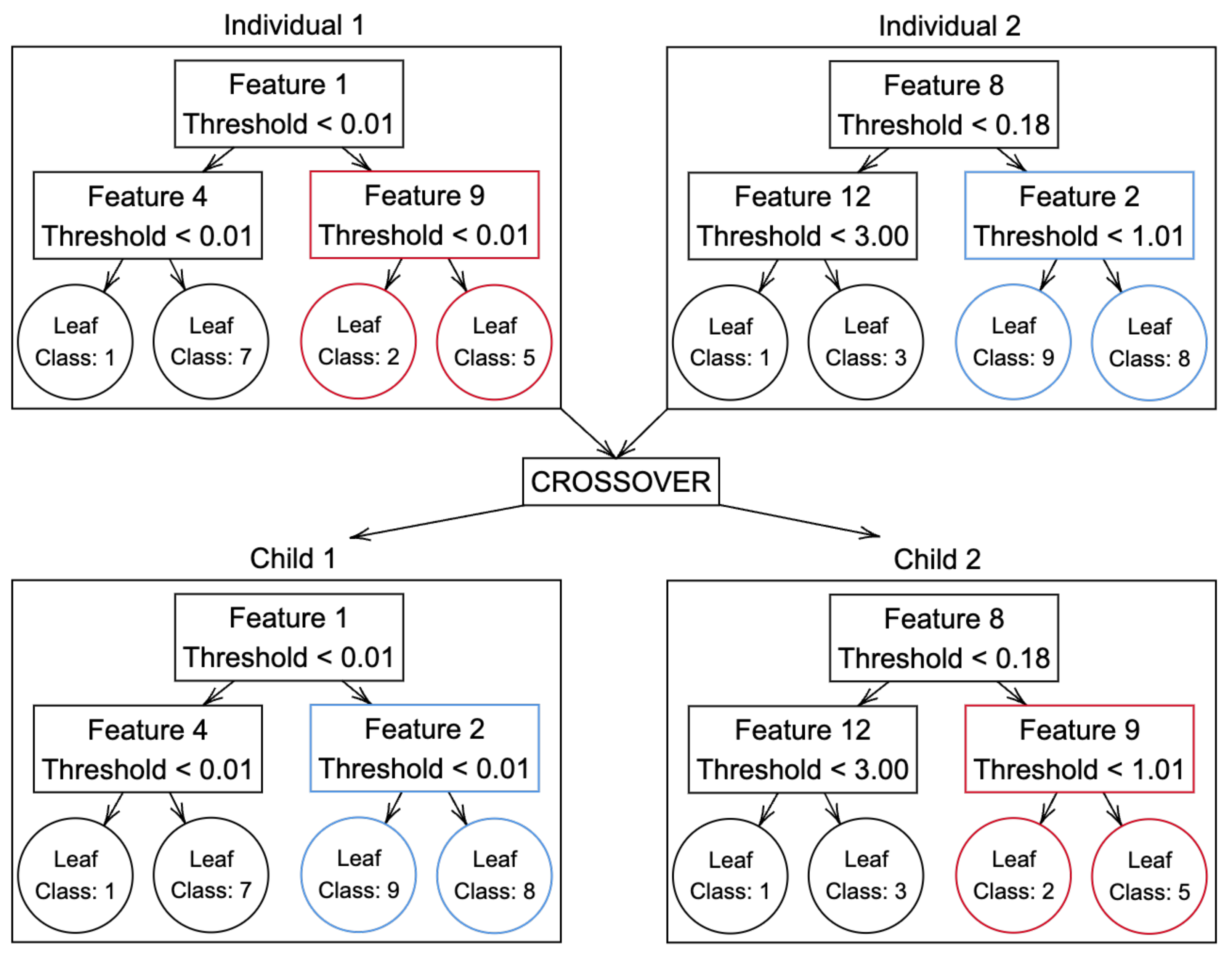
Following the completion of tournaments and the formation of the winners’ list, the crossover stage between individuals commences. In this phase, two individuals are randomly selected from the list of winners for possible crossover. If the crossover probability is equal to or exceeds the defined crossover rate, the crossover operation takes place; otherwise, the two selected individuals are returned without undergoing crossover. In the event of a crossover, the two individuals are segmented at one or more random points, and these segments are exchanged between them, generating two new offspring individuals. This crossover process iterates until half of the population has undergone a crossover, resulting in an equal number of new individuals. The pairs of resulting individuals from each crossover are then integrated into the list of the new generation, thereby constituting a fresh generation of individuals. Figure 4 visually illustrates the crossover process.

3.5. Mutation

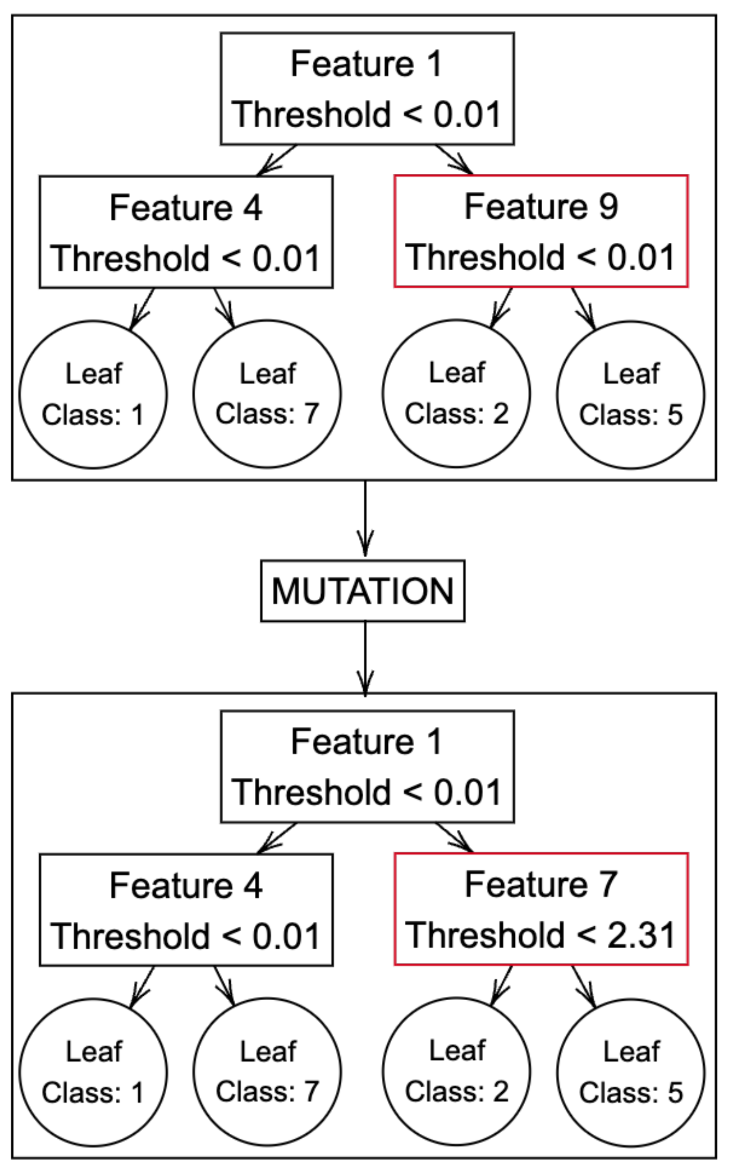
Following the establishment of the new generation, each individual has the opportunity to undergo the mutation process, a pivotal stage for injecting genetic diversity into the population and exploring novel solutions. Mutation rate, a user-defined parameter, governs the likelihood that an individual will undergo mutation. If a randomly generated decimal number between 0 and 1 exceeds or equals the mutation rate, the individual undergoes mutation.

In the mutation process, a node within the tree is randomly chosen. Subsequently, both the attribute and the threshold of this node undergo random modifications. If the selected node is a leaf node, the associated target class is subject to random alteration. This involves randomly selecting a target class from the dataset and assigning it to the leaf node, thereby introducing variability into the tree structure. This iterative process empowers the population to explore different paths and potentially uncover more effective solutions to the classification problem [38]. The mutation process is visually depicted in Figure 5.

3.6. Elitism

Following the formation of the new generation of individuals, the elitism technique is employed with the explicit goal of safeguarding the finest individual from the preceding population. This strategic approach is put in place to avoid a quick decline in the quality of the population in future generations.

In the elitism process, the person with the lowest fitness in the new generation is replaced by the best-performing individual from the prior generation. Effectively, this means that the least-adapted individual from the recent generation is discarded, while the most adept individual from the previous generation is retained within the current population. This deliberate strategy ensures the preservation of the advantageous traits exhibited by the top-performing individual of the previous generation, thereby contributing to a more stable and consistent population evolving over time [39].

3.7. Exchange

In scenarios involving multiple populations during the execution of the algorithm, there exists a mechanism wherein the best individuals or random individuals from one population may migrate to another. This interpopulation migration is contingent upon the exchange rate, a user-defined parameter that denotes the probability of such transfers occurring.

For example, consider a situation with two populations. If a randomly generated number between 0 and 1 exceeds or equals the exchange rate, migration begins. In this process, the best individual from one population may migrate to the other, and vice versa.

The migration approach has the potential to be a useful tool in fostering increased similarity among individuals. When individuals move from one population to another, they may encounter more genetic variation than those staying in their original population. This can result in a higher chance of finding better solutions. Additionally, this approach may be notably effective in mitigating challenges posed by local maxima, introducing a mechanism to circumvent stagnation in population evolution by facilitating the exchange of individuals between populations, allowing the algorithm to explore varied regions within the search space and potentially evading entrapment in a local optimum.

3.8. Fault Detection and Isolation

The proposed FDI system consists of two main components: the change point detection module (for fault detection) and the decision trees induced by the genetic programming diagnosis module. The FDI procedure shown in Algorithm 3 is applied to sliding windows, and each window is associated with a variable measurement.

Algorithm 3 FDI Algorithm

4. Case Study: FDI in the Tennessee Eastman Process

The FDI strategy was applied in the Tennessee Eastman (TE) process simulator [35]. According to [40], the TE process results in two products (G and H) and one (undesired) by-product F from four reactants (A, C, D, and E). All reactions are irreversible, exothermic, and first-order approximately with respect to the reactants’ concentration. Moreover, the production of G requires greater temperature sensitivity to have a higher activation energy. Figure 6 shows a flow sheet of the Tennessee Eastman (TE) process. There are five unit operations: reactor, condenser, vapor–liquid separator, recycle compressor, and stripper.

The process variables are categorized into faults, inputs, and outputs, as presented in Table 1. In this study, we utilized the training and test data provided by the Braatz Group at MIT (available at http://web.mit.edu/braatzgroup/TE_process.zip accessed on 12 April 2024), as described by [26] and [41]. Additionally, the dataset underwent cleansing following the methodology outlined in [40], where variables exhibiting high correlation or remaining static were excluded.

• Highly correlated: XMEAS(13), XMEAS(16), XMEAS(19-22), XMEAS(33), XMV(3), and XMV(5-11)
• Static: XMEAS(5-6), XMEAS(12), XMEAS(14-15), XMEAS(17), and XMV(4)

Table 1. Process faults and input and output variables for the Tennessee Eastman process simulator.

Process Faults		Output Variables
Name	Description	Name	Description
IDV (1)	A/C feed ratio, B composition constant  (s4)	XMEAS (1)	A feed  (s1)
IDV (2)	B composition, A/C ratio constant  (s4)	XMEAS (2)	D feed  (s2)
IDV (3)	D feed temperature  (s2)	XMEAS (3)	E feed  (s3)
IDV (4)	Reactor cooling water inlet temperature	XMEAS (4)	A and C feed  (s4)
IDV (5)	Condenser cooling water inlet temperature	XMEAS (5)	Recycle flow  (s8)
IDV (6)	A feed loss  (s1)	XMEAS (6)	Reactor feed rate  (s6)
IDV (7)	C header pressure loss  (s4)	XMEAS (7)	Reactor pressure
IDV (8)	A, B, C feed composition  (s4)	XMEAS (8)	Reactor level
IDV (9)	D feed temperature  (s2)	XMEAS (9)	Reactor temperature
IDV (10)	C feed temperature  (s4)	XMEAS (10)	Purge rate  (s9)
IDV (11)	Reactor cooling water inlet temperature	XMEAS (11)	Product separator temperature
IDV (12)	Condenser cooling water inlet temperature	XMEAS (12)	Product separator level
IDV (13)	Reaction kinetics	XMEAS (13)	Product separator pressure
IDV (14)	Reactor cooling water valve	XMEAS (14)	Product separator underflow  (s10)
IDV (15)	Condenser cooling water valve	XMEAS (15)	Stripper level
IDV (16)	Unknown	XMEAS (16)	Stripper pressure
IDV (17)	Unknown	XMEAS (17)	Stripper underflow  (s11)
IDV (18)	Unknown	XMEAS (18)	Stripper temperature
IDV (19)	Unknown	XMEAS (19)	Stripper steam flow
IDV (20)	Unknown	XMEAS (20)	Compressor work
IDV (21)	The valve for s4 was fixed at steady state	XMEAS (21)	Reactor cooling water outlet temperature
		XMEAS (22)	Separator cooling water outlet temperature
Input Variables		XMEAS (23)	Reactor feed analysis  (s6) Comp. A
Name	Description	XMEAS (24)	Reactor feed analysis  (s6) Comp. B
XMV (1)	D feed flow  (s2)	XMEAS (25)	Reactor feed analysis  (s6) Comp. C
XMV (2)	E feed flow  (s3)	XMEAS (26)	Reactor feed analysis  (s6) Comp. D
XMV (3)	A feed flow  (s1)	XMEAS (27)	Reactor feed analysis  (s6) Comp. E
XMV (4)	A and C feed flow  (s4)	XMEAS (28)	Reactor feed analysis  (s6) Comp. F
XMV (5)	Compressor recycle valve	XMEAS (29)	Purge gas analysis  (s9) Comp. A
XMV (6)	Purge valve  (s9)	XMEAS (30)	Purge gas analysis  (s9) Comp. B
XMV (7)	Separator pot liquid flow  (s10)	XMEAS (31)	Purge gas analysis  (s9) Comp. C
XMV (8)	Stripper liquid product flow  (s11)	XMEAS (32)	Purge gas analysis  (s9) Comp. D
XMV (9)	Stripper steam valve	XMEAS (33)	Purge gas analysis  (s9) Comp. E
XMV (10)	Reactor cooling water flow	XMEAS (34)	Purge gas analysis  (s9) Comp. F
XMV (11)	Condenser cooling water flow	XMEAS (35)	Purge gas analysis  (s9) Comp. G
XMV (12)	Agitator speed	XMEAS (36)	Purge gas analysis  (s9) Comp. H
		XMEAS (37)	Product analysis  (s11) Comp. D
		XMEAS (38)	Product analysis  (s11) Comp. E
		XMEAS (39)	Product analysis  (s11) Comp. F
		XMEAS (40)	Product analysis  (s11) Comp. G
		XMEAS (41)	Product analysis  (s11) Comp. H

Table 1. Process faults and input and output variables for the Tennessee Eastman process simulator.

Process Faults		Output Variables
Name	Description	Name	Description
IDV (1)	A/C feed ratio, B composition constant  (s4)	XMEAS (1)	A feed  (s1)
IDV (2)	B composition, A/C ratio constant  (s4)	XMEAS (2)	D feed  (s2)
IDV (3)	D feed temperature  (s2)	XMEAS (3)	E feed  (s3)
IDV (4)	Reactor cooling water inlet temperature	XMEAS (4)	A and C feed  (s4)
IDV (5)	Condenser cooling water inlet temperature	XMEAS (5)	Recycle flow  (s8)
IDV (6)	A feed loss  (s1)	XMEAS (6)	Reactor feed rate  (s6)
IDV (7)	C header pressure loss  (s4)	XMEAS (7)	Reactor pressure
IDV (8)	A, B, C feed composition  (s4)	XMEAS (8)	Reactor level
IDV (9)	D feed temperature  (s2)	XMEAS (9)	Reactor temperature
IDV (10)	C feed temperature  (s4)	XMEAS (10)	Purge rate  (s9)
IDV (11)	Reactor cooling water inlet temperature	XMEAS (11)	Product separator temperature
IDV (12)	Condenser cooling water inlet temperature	XMEAS (12)	Product separator level
IDV (13)	Reaction kinetics	XMEAS (13)	Product separator pressure
IDV (14)	Reactor cooling water valve	XMEAS (14)	Product separator underflow  (s10)
IDV (15)	Condenser cooling water valve	XMEAS (15)	Stripper level
IDV (16)	Unknown	XMEAS (16)	Stripper pressure
IDV (17)	Unknown	XMEAS (17)	Stripper underflow  (s11)
IDV (18)	Unknown	XMEAS (18)	Stripper temperature
IDV (19)	Unknown	XMEAS (19)	Stripper steam flow
IDV (20)	Unknown	XMEAS (20)	Compressor work
IDV (21)	The valve for s4 was fixed at steady state	XMEAS (21)	Reactor cooling water outlet temperature
		XMEAS (22)	Separator cooling water outlet temperature
Input Variables		XMEAS (23)	Reactor feed analysis  (s6) Comp. A
Name	Description	XMEAS (24)	Reactor feed analysis  (s6) Comp. B
XMV (1)	D feed flow  (s2)	XMEAS (25)	Reactor feed analysis  (s6) Comp. C
XMV (2)	E feed flow  (s3)	XMEAS (26)	Reactor feed analysis  (s6) Comp. D
XMV (3)	A feed flow  (s1)	XMEAS (27)	Reactor feed analysis  (s6) Comp. E
XMV (4)	A and C feed flow  (s4)	XMEAS (28)	Reactor feed analysis  (s6) Comp. F
XMV (5)	Compressor recycle valve	XMEAS (29)	Purge gas analysis  (s9) Comp. A
XMV (6)	Purge valve  (s9)	XMEAS (30)	Purge gas analysis  (s9) Comp. B
XMV (7)	Separator pot liquid flow  (s10)	XMEAS (31)	Purge gas analysis  (s9) Comp. C
XMV (8)	Stripper liquid product flow  (s11)	XMEAS (32)	Purge gas analysis  (s9) Comp. D
XMV (9)	Stripper steam valve	XMEAS (33)	Purge gas analysis  (s9) Comp. E
XMV (10)	Reactor cooling water flow	XMEAS (34)	Purge gas analysis  (s9) Comp. F
XMV (11)	Condenser cooling water flow	XMEAS (35)	Purge gas analysis  (s9) Comp. G
XMV (12)	Agitator speed	XMEAS (36)	Purge gas analysis  (s9) Comp. H
		XMEAS (37)	Product analysis  (s11) Comp. D
		XMEAS (38)	Product analysis  (s11) Comp. E
		XMEAS (39)	Product analysis  (s11) Comp. F
		XMEAS (40)	Product analysis  (s11) Comp. G
		XMEAS (41)	Product analysis  (s11) Comp. H

4.1. Results

The Tennessee Eastman process simulator dataset was partitioned into two distinct sections for the fault detection and isolation (FDI) system—one designated for training and the other for testing purposes. The training dataset served as the basis for generating 730 vectors through the fault detection system’s change point detection module. This module analyzed 10 simulations for each fault, reading sensors within the Tennessee Eastman benchmark process. It extracted measurement windows, comprising time series utilized in a fuzzy/Bayesian approach to determine the likelihood of change point occurrences across the time series.

The results obtained from the change point detection module were integrated into a decision tree induced by genetic programming. This decision tree was instrumental in classifying the 21 faults, constituting a novel approach to fault diagnosis. Following the implementation of the algorithm, performance evaluations were carried out through a series of tests. The database was stratified into training and testing sets using a 70% allocation for training and 30% for testing. Additionally, specific parameters were configured as follows:

• Maximum tree depth: 100;
• Number of generations: 1000;
• Population size: 100 individuals;
• Crossover rate: 0.9;
• Mutation rate: 0.4;
• Elitism enabled;
• Tournament selection with two competing individuals;
• Multi-point crossover;
• Population amount: 2.

In these configurations, we performed 100 executions of the diagnostic algorithm and computed the average results. The following summarizes our findings:

• Average runtime: 02:19:14;
• Average number of features used: 29.65;
• Median tree depth: 37.68;
• Average number of nodes: 150.32;
• Average training accuracy: 0.8148;
• Average test accuracy: 0.8043;
• Average training standard deviation: 0.0311;
• Average testing standard deviation: 0.0365.

The analysis of the average accuracy across distinct classes highlights the inherent complexity of the classification problem under consideration, characterized by a multitude of classes. It is crucial to recognize that, despite the significant variety of classes, the algorithm demonstrated impressive performance in many cases. The classification task involves a wide range of categories, each representing a distinct class, which presents a notable challenge requiring strong discrimination and generalization abilities.

Interestingly, multiple classes consistently achieved exceptional accuracy levels, exceeding the threshold of 90%. This attestation underscores the algorithm’s capacity for precise and reliable classifications across diverse categories, even in the face of the intricate nature of the problem. Although certain classes manifested moderate or lower accuracies, it is essential to recognize the inherent challenges associated with distinguishing between multiple classes, leading to occasional classification difficulties. However, the algorithm demonstrated resilience by generating correct predictions in these instances, highlighting its adaptability across a spectrum of scenarios.

Especially noteworthy is the most effective test iteration, which yielded an average training accuracy of 0.8762 and an average test accuracy of 0.8724. These results signify a noteworthy accomplishment, showcasing the algorithm’s adeptness in learning and generalizing across disparate datasets. Despite the challenges encountered in certain classes, it is pivotal to underscore the algorithm’s success in classes with notably high accuracies. These positive outcomes reflect the efficacy of the model in providing accurate classifications across a diverse array of situations.

4.2. Result Comparison

The average accuracy outcomes of this study were contrasted with those of the study suggested in [27].

Table 2. Comparison of correctness (%) between the proposed methodology, PCA, and SVM.

Description	Proposed Methodology	PCA	SVM
Fault 1	99.27%	87.19%	87.19%
Fault 2	96.43%	87.50%	85.83%
Fault 3	50.67%	18.33%	15.21%
Fault 4	67.16%	72.71%	49.48%
Fault 5	97.45%	4.06%	50.60%
Fault 6	94.33%	90.21%	78.85%
Fault 7	93.17%	89.69%	88.85%
Fault 8	98.66%	85.00%	32.19%
Fault 9	9.84%	20.00%	12.00%
Fault 10	94.95%	76.15%	22.60%
Fault 11	74.37%	65.42%	11.88%
Fault 12	98.73%	85.83%	50.21%
Fault 13	91.78%	69.06%	21.46%
Fault 14	86.80%	86.56%	54.90%
Fault 15	88.94%	23.02%	18.85%
Fault 16	75.81%	69.48%	12.81%
Fault 17	90.06%	74.48%	48.02%
Fault 18	62.58%	59.90%	32.19%
Fault 19	89.15%	84.06%	46.25%
Fault 20	80.84%	77.50%	38.96%
Fault 21	45.78%	85.00%	8.23%
Mean	80.32%	67.20%	41.26%

shows this comparison.

Table 2 enumerates the correction rates in various fault classes within the Tennessee Eastman Process Simulation Dataset, providing a comparative analysis of three distinct methodologies: the approach proposed in this study, principal component analysis (PCA), and support vector machines (SVMs).

The proposed methodology presented a spectrum of correction rates, ranging from 9.84% to 98.73%, with an average of 80.32%. Remarkably high correction rates were observed for specific fault classes, such as faults 1, 5, and 12, recording rates of 99.27%, 97.45%, and 98.73%, respectively. On the contrary, certain fault classes, including faults 3, 9, and 21, exhibited comparatively reduced correction rates.

Principal component analysis manifests varied correction rates, ranging from 4.06% to 90.21%, with an average of 67.20%. While notable improvements were seen in certain fault categories using PCA, there were evident difficulties that reflected the patterns noted in the suggested approach.

Support vector machines exhibited a broad spectrum of correction rates, ranging from 8.23% to 88.85%, with an average of 41.26%. The efficacy of SVM in specific fault classes was juxtaposed with lower correction rates observed in others.

Upon comprehensive scrutiny, the comparative analysis underscores that the methodology proposed in this study generally achieved superior correction rates across a majority of fault classes within the Tennessee Eastman Process Simulation Dataset when contrasted with PCA and SVM.

5. Conclusions

This paper introduces an innovative data-driven fault detection and isolation (FDI) methodology. The proposed FDI system comprises two key modules: (i) a change point indicator, leveraging the Metropolis–Hastings algorithm in conjunction with fuzzy set theory, to detect alterations in time series and furnish evidence of potential faults (fault detection) and (ii) a novel approach utilizing a decision tree induced by genetic programming for fault classification. In particular, the methodology distinguishes itself by not necessitating mathematical or statistical models, thereby mitigating the intricacies associated with implementation. The proposed method generalizes the one-class GP-induced decision tree model to effectively address challenges associated with multiclass classification. It introduces a strategy involving the simultaneous evolution of multiple parallel populations.

To assess its efficacy in a real-world context, we employed the renowned Tennessee Eastman benchmark process. In this case study, the proposed approach demonstrated effectiveness and feasibility for fault detection and classification in complex industrial systems, with the potential for further enhancements in interpretability and handling challenging fault classes. The technique achieved around 80% correct predictions, showing capability for reliable classifications across various fault categories and outperforming alternative methods like PCA and SVM in correction rates across multiple fault classes within the Tennessee Eastman dataset.