
Global Stabilizing Control of a Continuous Ethanol Fermentation Process Starting from Batch Mode Production


Faculty of Chemical Engineering, Kunming University of Science and Technology, Kunming 650500, China
*
Author to whom correspondence should be addressed.
Processes 2024, 12(4), 819; https://doi.org/10.3390/pr12040819
Submission received: 23 March 2024
/
Revised: 14 April 2024
/
Accepted: 17 April 2024
/
Published: 18 April 2024
(This article belongs to the Section Biological Processes and Systems)
Abstract
:Traditional batch ethanol fermentation poses the problems of poor production and economic viability because the lag and stationary phase always demand considerable fermentation time; plus, downtime between batches is requested to harvest, clean, and sterilize, decreasing the overall productivity and increasing labor cost. To promote productivity and prolong the production period, avoid process instability, and assure a substantial production of ethanol and a minimal quantity of residual substrate, this paper proposed a nonlinear adaptive control which can realize global stabilizing control of the process starting from batch mode to achieve batch/washout avoidance. Due to the dynamic nature and complexity of the process, novel estimation and control schemes are designed and tested on an ethanol fermentation model. These schemes are global stabilizing control laws including adaptive control to avoid input saturation, nonlinear estimation of the unknown influential concentration through a higher-order sliding mode observer, and state observers and parameter estimators used to estimate the unknown states and kinetics. Since the temperature is an important factor for an efficient operation of the process, a split ranging control framework is also developed. To verify the process performance improvement by continuous fermentation, tests performed via numerical simulations under realistic conditions are presented.
1. Introduction
With the growth of the bio-manufacturing industry, the design of bio-conversion systems has drawn considerable attention due to their potential to improve production efficiency, plant profitability, and sustainability [1,2]. As a renewable source of fuel, ethanol represents a great opportunity to help meet future energy demands and reduce greenhouse gas (GHG) emissions. Consequently, the production of ethanol has been attracting plenty of interest from all over the world, especially with the breakthroughs in the pretreatment and enzymatic hydrolysis of lignocellulosic feed-stocks that hold an annual yield of about 180 billion tons [3] worldwide.
Despite well-recognized technical barriers to viable commercialization of bio-ethanol having been overcome, the fermentation process itself is now identified as a limiting factor and poses a multi-scale challenge. First of all, current fermentation is mainly batch/fed-batch based, which demands intensive labor for both prior- and post-production; plus, the lag and stationary phase occupies considerable time, causing relatively low productivity. The second challenge is on the design of suitable mathematical models to describe this complex bioprocess; and because bioprocesses use living microorganisms that act as biocatalysts, they are sensitive to extracellular environment, and obtaining accurate and reasonably priced sensors for real-time measurement of the bioprocess variables utilized in the control systems is problematic [4,5,6]. Moreover, appropriate design of the regulator demands strict and multidimensional defining of critical process parameters for the used microorganism strain, but start-up or maintaining the bioreactor is a long-term process during which objectives, physicochemical variables, and dynamic behavior can be changed by the operator. Nonetheless, the International Energy Agency [7] forecasts that in 2050, 27% of the global transport fuel can be sustainably supplied from biomass and waste resources. As a result, the ethanol fermentation process design and optimization are inherently synergistic and multidisciplinary.
The design of the fermentation configuration is expected to improve metabolic intensity, increase productivity, and accelerate substrate conversion. Correspondingly, continuous culturing eliminates downtime between batches, as well as the requested interval to harvest, clean, and sterilize; hence, this intensifies production and reduces labor cost. By chemostats or turbidostats, a continuous culture device dilutes cells and waste products at the same rate that they are being produced. But a typical drawback of the continuous fermentation is the presence of multiple outputs (which would easily shift the process to the washout condition), as well as oscillations under certain conditions (the effect being the decrease in ethanol productivity, the loss of a high quantity of substrate). To stabilize the process, the cause of the reactor instability [8,9,10,11,12] is investigated; and, in view of the fact that the osmotic pressure formed at high ethanol concentrations (~50–60 g/L [13,14]) might inhibit or even kill yeast cells, hybrid designs through in situ ethanol removal to alleviate ethanol stress [15] are proposed. However, the accompanied instrumental cost as well as possible membrane fouling and degeneration are unbearable in industry.
On the other hand, formulating a feedback control loop through manipulating dilution rate, dissolved oxygen level, pH, or inlet substrate concentration [16,17,18,19,20,21,22,23] to eliminate the fermentation–separation mismatch is a cost-effective way to stabilize the process. The research in this domain is oriented both to the developing of suitable mathematical models and to the design of appropriate monitoring and control strategies able to assure the stability. To summarize, the ethanol fermentation process is influenced by a number of parameters, such as temperature, substrate, pH value, fermentation time, mixing speed, and inoculum size, as well as the concentration of ethanol in the system [24]. Hence, the system to control is multidimensional and complex, and their models contain kinetic parameters that are uncertain and time-varying. A number of stabilization techniques necessitate software sensors for the estimation of biological states, kinetic parameters, and even kinetic reactions based on detectable signals. However, the estimation of input substrate concentration is a difficult task in practice, the input conditions are unknown and time-varying because of upstream disturbances, especially for the continuous production mode where a series of CSTR tanks are connected to decrease the overall substrate run-off.
Observer-based estimation of the fermenter states and kinetics with limited on-line measurements and knowledge of the process model information could minimize the capital cost of the formulated closed-loop system, but process–model mismatch is an in-avoidable factor. Moreover, the control objectives become fuzzy as the main biological state variables vary extremely slowly; for instance, the duration of one batch fermentation that account for 87% of the world ethanol production scale is about 60–72 h, where almost no control intervention is added in classic flow-sheet. To clarify the objectives to control, intensive experimental and theoretical research [25] applications concentrate on growing cultures under different conditions in order to properly characterize the microorganisms and to find optimum productivity. To make the most profit from the process, it is also demanded to minimize the transition time between consecutive steady state operating points. For this reason, global stability is essential for their successful control.
To approach maximum metabolic intensity, this paper works on global stabilizing control (GSC) of the fermentation process which starts from batch mode, and the control is implemented to prolong the production period, where the ladder pattern trajectory of substrate concentration is tracked to approximate toward the unknown substrate consumption capabilities. Previously reported GCS approaches are mainly linearizing controllers [26], but the main drawback of these global approaches is that they use perfect model knowledge. Other global control techniques assuming model uncertainties arise [27], using interval observers’ results. However, a drawback common to most of the aforementioned control strategies is that they often do not explicitly take into account the non-negativity constraints on the manipulated variables.
In this paper, a globally adaptive feedback law is adopted that the feedback gain dynamically adapted in such a way that control never saturates, and the unknown input substrate concentration is explicitly related in the control law to accommodate the time-varying disturbance. For reconstructing the unknown states and disturbed input concentration information from the measurements of ethanol and substrate concentrations, a sliding-mode observer (SMO) is derived. The design of state observers and parameter estimators depends on the information provided on-line by the previous. The distinguishing properties of the discontinuous generalized super-twisting observer (GSTO) compared to other smooth observers are convergence in finite time and insensitivity to time-varying but bounded perturbations [28].
The paper is organized in the following manner. Section 2 describes the fermentation process model, and possible monitoring/control problems under different operation modes are discussed; this is followed by the development of adaptive estimation and control in Section 3; in Section 4, experiment validation is conducted on the ethanol fermentation process, and adaptive control under unknown inputs and undetectable states is implemented in this MIMO system, where to obtain optimal state references the system starting in batch mode is regulated using the technique of global stabilizing control; finally, Section 5 concludes the paper.
2. Problem Formulation
In this paper, a continuous fermentation process of Saccharomyces cerevisiae used to produce ethanol is studied; subsequent investigation on batch mode production is realized by manipulating input/output flow rates (or dilution rate) synchronously. As is shown in Figure 1, a flow Fin of culturing broth containing substrate Sin is continuously fed into the reactor, the volume V is held constant when the outflow Fout = Fin. The jacket with control (Vj, Tinj, Fj) could maintain the reactor temperature Tr as desired. We assume the content is well-mixed with one substrate-limited material (e.g., glucose) feeding in continuously for the growth of biomass/yeast, and the same amount of broth liquor is removed to acquire the product ethanol.
The nonlinear dynamics of the studied process [29] in Figure 1 can be obtained based on the mass balance of the substrate (S), biomass (X), and product (P) as follows,
where Fin = Fout = F, and D = F/V is the dilution rate defined as the reciprocal of the reactor space–time for the culturing media, which is the control action used to determine the operating status of the chemostat. One crucial problem in solving Equation (1) is the formulation of expressions for the kinetic functions r1(·) and r2(·), which could be a large number of analytical expression candidates. Note that in practical applications, actuators could be adopted to create the control action D, and their dynamics will be considered in Section 4.1.
In practice, fermenter control design should consider realistic conditions related to process inputs, state variables, and reaction kinetics, as well as possible control to enhance substrate conversion and the production rate. Without a loss of generality, the following performance requirement and assumption are considered.
- Monitoring Information: The quantity r2(·) is available on-line from the plant, and for a large part of bioprocesses, the production (or consumption) of gaseous components, as peculiar to ethanol fermentation by S. cerevisiae, CO2 is monitored and is directly related to r2(·), and the accumulation of CO2 evolution rate (CER) is proportional to P when D is fixed.
- Dynamic Heat Balance of the Jacketed Fermenter: In order to assure a hospitable environment, fermentation temperature is regulated to maintain at an optimum. The aerobiotic respiration effect might cause exothermic reactions and a jacket cooler is integrated to remove redundant heat, and heat transfer between the broth and coolant is rendered as perfect convection,where ΔHr is the mole enthalpy change in the oxidation reaction; KTAT is the heat transfer coefficient multiples area of heat exchange. Note that O2 from the sterilized air is dissolved into the broth and transported by input effluents, and the aerobiotic effect of yeast leads to exothermic reactions. Dissolved oxygen (DO) content in the electrolyte solution is influenced by pH, Tr, and the global effect of ionic strength ∑HkIk,where ∑HkIk is accounted as [28,29] follows,
- 3.
- Temperature influence on the kinetics: The maximum specific growth rate μm is correlated with the broth temperature which is provided in the form of the Arrhenius formula,where Ea1 and Ea2 are the activation energy, and A1 and A2 are the preexponential factors.
Remark 1.
Systems (1)–(5) have been widely used to represent essential characteristics of the continuous fermentation process. Some advanced controllers have been proposed to regulate temperature and the states [30] and references therein. However, fermentation is an accumulative process where the substrate conversion rate/productivity is extremely slow, prescribed set-point tracking is challenged both on stability of the control law, as well as the adequacy for productivity increase. In view that there exists a maximum handling capability for microorganisms, the control objective of the chemostat is set as the ladder pattern, and the fermentation starts as batch mode and by so tracking, the period is prolonged to intensify productive, and by trial-and-error, maximum substrate conversion capability is obtained. To realize such a control, GSC is mandatory.
Remark 2.
Controlling tends to stabilizing, and a primary tool for culturing cells in a static environment is continuous culture, where inoculated growth medium is continually diluted with fresh medium. At steady state, a continuous culture device will dilute cells and waste substrates at the same rate that they are being produced leading to an unchanging environment [31]. To alleviate substrate run-off, industrial practice adopts CSTRs in series, and the input state Sin for a given fermenter becomes unknown and time-varying, biomass content X is not measurable on-line, and the biomass growth rate r(·) is completely unknown and time-varying because of uncertainties related to the maximum specific growth rate μm and of unavailability of X. Moreover, the control expects ethanol concentration and substrate conversion rate, as well as bio-conversion rate to be optimal, but non-linearity of the process might drive the system to washout condition and terminates the fermentation process. Hence, adaptive control related to the optimal status is to be achieved. It should be noted that X, rO2, and r1(·) are nonlinear and also unknown in this paper, which will be estimated on-line with observers.
3. Controller and Estimator Design
In this section, a GSC is proposed for (1) and (2) to regulate fermentation states and temperature. The optimal control of fermentation states is realized through the shifting of batch mode to continuous mode production; and, by ladder pattern trajectory tracking, the maximum substrate conversion rate of the fermenter is obtained and controlled. For the control of temperature, feedback linearization is adopted because we render measurement and modeling of the fermenter temperature which is corrected. Both above-mentioned controls need to consider bioreactor requirements like DO content, biomass X, and the time-varying substrate input concentration Sin.
3.1. Global Stabilizing Control
Demanding on the control purpose, we want to globally regulate the fermentation states [S, X, P], but ethanol is viewed as primary metabolite and the kinetics r1 and r2 becomes correlative, which leads the values of X and P obtained at equilibrium are completely determined by the value of the targeted set point Sref for substrate concentration. Then, we will only focus on regulation of S in this work.
Sref ∈ (0, Sin) denotes the desired set points; the corresponding positive equilibrium values are Pref = r2YSXYSP(Sin − Sref)/(r1YSP + r2YSX) and Xref = r1YSXYSP(Sin − Sref)/(r1YSP + r2YSX). The objective is to formulate a control D(·) to globally stabilize (1) towards the reference [Sref, Pref, Xref]. We set β = r1/r2, and the nonlinear control law is obtained,
which formulates the following closed-loop system,
Since [S, X, P] is positively invariant, for any initial state conditions with physical meaning, the control D(·) ≥ 0, integrating Equation (7), and we show that for any t ≥ 0,
Hence, the control law (6) is bounded below by a positive constant; plus, (7) provides [Sref, Pref, Xref] as globally exponentially stable. To mention, (6) is the nonlinear control that is difficult to realize through error dS = Sref − S reduction, and the linearization control of a chemostat based on (6) towards any a set-point Sref, even unreachable in open-loop, is also globally stabilizable, which is similarly rephrased by the following fermenter temperature control.
In this paper, we adopt the linearization control of fermenter temperature using jacket flow Fj as the manipulated variable. We assume the model (2) is precise and full knowledge of temperature measurement is available. Firstly, given that the jacket volume Vj is orders smaller than the fermenter volume V, the quasi-steady state obtains,
which substituted in the first formula gives
and by the form of variation, Equation (10) provides the transfer relation,
where δTr = Trref − Tr. Moreover, the equilibrium at the reference provides,
We replace Equation (10) with Equations (11) and (12) and the exact linearization control gives,
Eliminating the derivatives, we have the control law as follows,
The closed-loop system adopting Equation (14) provides,
and when the tuning parameter η is positive, the closed-loop system is globally stabilizable.
Remark 3.
Regulating the chemostat by the following linearization control is also globally stabilizable,
However, the controller proposed in (16) requires perfect knowledge of the dynamic system, and an adaptive feedback control law based on on-line information from the plant is provided.
Theorem 1.
Assume the kinetics r2 is monitored on-line by CER and follows y1 = λr2, the adaptive control law,
globally stabilizing (1) towards the positive set points [Sref, Pref, Xref, γref], where γref = (β/YSX + 1/YSP)/λ/(Sin − Sref).
Proof.
Control law (17) yields to the closed-loop system,
Consider the positive initial condition plus γ(0) ∈ (γm, γM); then, γ is bounded similar to (8),
Since y1 = λr2 is bounded below a positive constant, a time change τ = ty1, and obtains the following standard control,
where υref = Sin − Sref. Since (20) is an autonomous triangular system, it is separable [32], and for the subsystem in υ and γ, the initial condition is confined to the set W = {υ > 0, γ ∈ (γm, γM)}; then, an analog can be performed that υ is viewed as the prey and γ as the predator, and the Lyapunov function is formulated,
We check that V(υ, γ) is defined, non-negative on W, and vanishes only on υ = υref and γ = γref, and
which is non-positive. From Lasalle’s theorem, (υref, γref) is a globally attractive fixed point, and so are (Xref, Pref), considering that (20) is the triangular system. Thus, moving back to the original time and state variables, the control law (17) globally stabilizes the system (1) towards the nominal reference represented by Sref. □
Remark 4.
In addition to the information of CER, control (17) also demands the substrate (glucose) content available on-line, which could be detected in real time using automated approaches, like near-infrared, Fourier transformed infrared and Raman spectroscopy, or soft sensors [33,34]. The detection of r2(·) is challenging, but for a large part of bioprocesses, the production/consumption of gaseous components (dissolved oxygen, CO2) is monitored and is directly related to kinetics. For yeast cell growth, CO2 is usually released form the fermenter as a by-product, and this makes CER another feedback control parameter for the control system, defined as follows,
where P is the pressure (atm), R is the ideal gas constant (atm·L/(mol·K)), T is the temperature of the venting gas mixture (K), V is the working volume of the liquid inside the fermenter (L), Q is the volumetric gas flow rate for the existing gas stream (L/h), CO2 gas out is the gaseous CO2 concentration read by a near-infrared sensor in the venting line of a fermenter, and CO2 air input is the gaseous CO2 concentration obtained from the constant air flow.
Remark 5.
The above control (17) is implemented on a chemostat where the substrate is measured and controlled; if the system is designed to regulate cell content X by turbidostats with the aid of an on-line OD600 sensor, we can build the adaptive control as follows,
Similarly, the regulation of P can also be developed with the same kind of adaption.
3.2. Observer-Based Estimation
Taking in account the whole knowledge concerning the process, the realistic conditions related to inputs, states, and reaction kinetics are listed in Figure 2: the input substrate concentration Sin is unknown and time-varying; the process state variable X is not measurable; the biomass growth rate r1(·), production rate r2(·), and oxygen consumption rate rO2(·) are unknown and time-varying because of uncertainties related to the maximum specific growth rate μm and X; the variables S, P, and CER are available on-line; the temperatures Tin and Tinj are time-varying.
3.2.1. Estimation of the Input Substrate Concentration
To facilitate the control of fermentation states, the input information Sin in (17) is mandatory, which might be unknown and time-varying when shifting to continuous mode. To alleviate residual substrate loss and upgrade ethanol content, common industrial practice adopts cascade fermentation with a series of tanks and partial reuse of end effluent, as is shown in Figure 3. For one casually assigned medial fermenter i in the series, problems arise as the input Sin is influenced by both upstream effluent and the supplement, causing the feed to be unknown and time-varying. Plus, it is assumed that the optimal set-point Sref is a function of Sin (since bio-conversion intensity is relatively constant for a given cell environment); hence, the reference might be time-varying if optimal operation of the process is expected. Hence, for the control of a fermenter i (labeled with red box), Sin is both unknown and time-varying, even Sin from saccharification section is fixed.
Based on the assumptions given in Figure 2, the estimation of the input substrate concentration is proposed. Firstly, ψ = S + P/YXP + X/YXS is constructed which gives dψ/dt = D(−ψ + Sin). Clearly, the auxiliary variable ψ is highly correlated with Sin through mass balance,
and when the initial states X0 and P0 approach zero, ψ and Sin are identical. From the state estimation perspective, the varying of Sin because of upstream disturbance could be reflected by changes in the time-derivative of ψ, and one can adopt observer-based estimation (OBE) on Sin through ψ.
Assuming ψ is available on-line, a linear observer is shown,
With appropriately designed gains κ1 > 0, the parameters κ2 > 0 and λψ > 0 are known to provide an exponentially convergent estimate of Sin in the absence of unknown perturbations. However, strict equivalence of Sin and ψ is inappropriate in practice and the deviation is manifested as unknown inputs. In synthesis, the linear observer (25) is not able to converge to the true value of the unmeasured states in the presence of unknown inputs. In fact, finite-time convergence is impossible for any observer having locally Lipschitz continuous perturbations, and convergence in the presence of persistent unknown inputs is also impossible for any continuous observer.
In order to alleviate the problem, SMO is introduced for trade-off of the perturbation terms, and to further estimate Sin correctly and obtain the convergent effect in finite time, the GSTO technique is adopted,
where μ1 > 0, μ2 > 0. The observer (26) is independent of the process kinetics and the tuning variables κ1, κ2, λψ, μ1, and μ2 are usually selected through a trial-and-error method. Comments can be drawn as follows: setting μ1 = 0 and μ2 > 0, (26) becomes a linear Luenberger observer, which can asymptotically estimate the true value only when Sin is constant. For varying inputs of substrate concentration, the estimation error of the linear observer is proportional to the size of the derivative and inversely proportional to the observer gains. The observer (26) could achieve finite-time convergence for an arbitrary Sin with bounded derivatives. The relative gain values suggested by Levant [35] are κ1 = 2.2 and κ2 = 1.5, which should be chosen to obtain good convergence with the GSTO algorithm. Finally, λψ affects both the convergence velocity and insensitivity to the change in Sin, as well as measurement noise.
3.2.2. Estimation of the Un-Measurable Biomass Concentration
To calculate ψ as well as the control (14) and (17), the biomass content X is needed besides the information of S and P. X is rendered difficult to measure on-line, and OBE is performed. Considering ethanol is the primary metabolite that is closely related to the content of biomass, X could be estimated through the construction of the observer on P. The procedure begins with the linearization of the subsystem in (1),
When (27) is non-singular, and D satisfies the persistent exciting (PE) condition, the non-biased estimation of P drives X to stably convergent to the real value [36]. In the following, a Luenberger observer is constructed for P,
where the hat represents the estimated value, and ω1 is the observer coefficient. For the estimated P to converge to the measured one, the right-hand side of Equation (28) needs to approach zero, and the variation form gives an estimation of X,
where γ1 is a positive tuning parameter. Combining (28) and (29), the OBE on biomass concentration is formulated.
3.2.3. Estimation of the Fermentation Kinetics
As it can be seen, the specific reaction rate r1 is involved for the aforementioned control and estimation, hence, estimation is performed in this section. Similar to the previous section, the OBE on r1 is obtained using the on-line measurement of substrate concentration.
where ω2 is another observer coefficient. And the estimator is given by,
where γ2 is another positive tuning parameter.
The same procedure is conducted for the estimation of rO2 with the aid of on-line detection on dissolved oxygen O2,
where ω3 and γ3 are positive tuning parameters. Note that the estimated rO2 is able to accomplish the temperature control law (14).
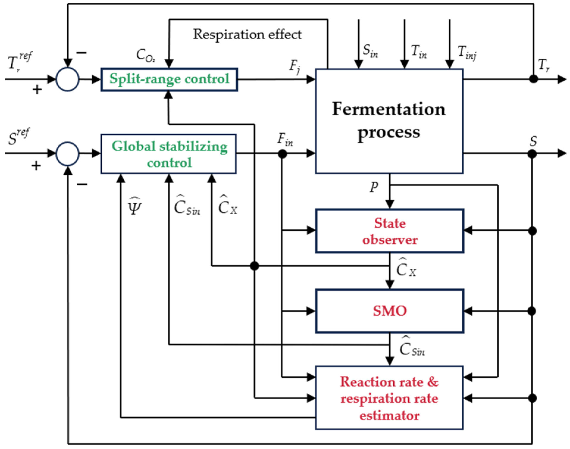
The schematic of the nonlinear control stat from batch mode production is shown in Figure 4. The control system contains two coupling loops, and the control laws are (14) and (17), respectively. For the temperature control, we assume the modeling is precise and the regulator adopts exact linearizing control as the backbone and the unknown or varying parameters are obtained using the techniques of OBE and GSTO. For the control substrate concentration, the nonlinear GSC technique is formulated and batch and washout avoidance are embedded.
4. Results and Discussion
In this section, fermentation that starts from batch mode is controlled with the expectation to prolong the production period, avoid process instability, and assure a substantial production of ethanol and a minimal quantity of residual substrate, meanwhile regulating the temperature inside the bioreactor at suitable values. We start from investigation on suitable mathematical models that describe the complex kinetics. Furthermore, since the fermentation process is an exothermic one, detailed regression to characterize heat balance is essential for the control system. Then, controls in the perfect model, as well as a possible process–model mismatch by introducing field data, are tested and discussed.
4.1. Fermentation Modeling Issues
Here, we introduce a benchmark example with complete known kinetics to investigate relations of the states against Sin, which together with their measurement units are presented in Table 1 [37],
However, considering the benchmark case is mainly applied for a scenario of continuous production, we regressed the kinetics (under 30 °C) using batch experiment data [37], and the updated parameters are listed Table 1. To regress the reaction kinetics, the mass conservation relation is revealed by YSX and YSP, which are obtained by fitting batch data; the kinetic parameters μm, Ks, and Ki are estimated using least squares regression of the integrated system (ode45 subroutine with the unknown parameters as the handle) against the field data, and the results are shown in Figure 5. Moreover, the empirical correlation of O2sat with varying Tr in Equation (3) is fitted under pH = 6 and represented as f(Tr) = 14.16 − 0.39Tr + 0.00772Tr2 + 0.000064Tr3 [38].
4.2. Analysis of the Open-Loop System
Before conducting quantitative analysis, the general system (1) is revisited for a glimpse of the open-loop system stability. For a given initial condition (S0, X0, P0), Equation (1) is well-posed and, since S(t → +∞) ≤ Sin < +∞, P(t → +∞) ≤ (1/YSP + β/YSX)Sin < +∞, and r2(., P) decreases with the increase in P, all non-negative set Ω = {(S, X, P): ≥0} values lie in the bounded set Ω eventually as time approaches infinity, indicating that the unlimited duplication of cells or sustained accumulation of ethanol is not possible. Note that output multiplicity exists for this system, where, apart from the trivial solution (Sin, 0, 0), we represent the non-trivial one as (S*, X*, P*), and the global stability property is provided by the following Theorem 2.
Theorem 2.
Assume r1/r2 = β is a constant, the stability criterion provides Dc < D, the travail solution (Sin, 0, 0) is asymptotically stable; Dc > D, the non-travail solution (S*, X*, P*) is asymptotically stable; Dc = D, both solutions are coincident and a branch point (BP) emerges, where Dc = r1(Sin, P)/X*.
Proof.
With a high-substrate environment and to avoid ethanol inhibition, β is viewed as a constant, X and P share identical dynamics, and (1) is reduced to second order. The equilibrium of the reduction system presents output multiplicity, and besides the travail solution (Sin, 0, 0), the non-trivial one gives,
As for the exploration of asymptotic behavior, we first implement dimensional reduction analysis. Laplace transform of the second and third formula in (1) gives,
which indicates that P(t) and X(t) share identical dynamic trajectories, and for any casually assigned initial states (X0, P0), the ethanol accumulation rate is proportional to the increase in yeast. Then, the characteristic equation of the limited system [S, X] provides,
Since λ1 = −D × (β/YSX + 1/YSP) is negative, local stability is determined by λ2 = μ − D, where μ(S, P) decreases with the increase of P because of the inhibitory effect. Moreover, the asymptotic property of the limiting system provides,
where f(P) is the product-inhibition term. Then, Fi(P) = μ(Sin − (β/YSX + 1/YSP)P)f(P) for i = 1, 2. Hence, Fi(0) = μ(Sin), Fi((β/YSX + 1/YSP)Sin) = 0, and Fi’(P) ≤ 0 if 0 ≤ P ≤(β/YSX + 1/YSP)Sin. The vector form gives,
when Dc = μ(Sin, P = 0) ≤ D, (0,0) is the only equilibrium and it is locally stable; when Dc > D, (X*, P*) = (DF2−1(D)/F1(F2−1(D)), F2−1(D)) is locally stable and (0, 0) becomes unstable.
When D = Dc, (X*, P*) degenerates to the washout condition. Substituting F(P) to system (24), one has,
By the Poincare–Bendixson theorem, the equilibrium is globally stable. □
In the following, process states with varying parameters D and Sin are analyzed. Although process–model mismatch is inevitable, quantitative analysis undertaken with fully known kinetics is essential because certain guidelines could be provided to aid in finding out optimal working conditions. As is shown in Figure 6, with the increase in D, P decreases rapidly till approaching zero, and the washout condition emerges and is labeled as BP, where all substrate is left unconsumed. For a given D, increasing Sin results in a limited effect on production P in the low D region, but the curves coincide at the high D region, which indicates that extra substrate supply is not constructive for process enhancement (Figure 6b). Moreover, the emergence of the washout condition is insensitive with varying Sin. Further plots of (Sin, S) and (Sin, P) reveal that the identical slope k exists when the substrate content is adequate, which means ΔS* is proportional to deviation of Sin, and from Equation (33) we have,
Since the limiting substrate is expected to be adequate in continuous fermentation, the (D, P) plots are identical with varying Sin, then, Δ(δP) = 0 and k = 1. In Equation (40), which indicates regulating substrate Sref under a chemostat by law (17) and regulating the cell number Xref using turbidostats in Remark 5, there are dual problems [39] so long as washout avoidance [40] conditions are promised.
To avoid washout, cell duplication should exceed cell loss, and the upper bound of D is provided as follows,
where ε ≥ 0 is the minimal allowable cell accumulation rate. To mention, ε is difficult to quantify in real applications. Hence, we provide to start the control from batch fermentation and GCS is implemented to promise shifting from a batch model to a continuous one. With the control law (17), D is unprovoked at the beginning and lasts for a while under very small initial γ0 = γ(t0 = 0), and the influence of varying Sin during this interval is avoided. To mention, the control starting by traditional batch mode production is easily applicable in practice, and after the cell is substantially accumulated, CER becomes detectable and r1 > 0 makes the actuator functional; then, with the bounded co-state γ, the control can track any reference Sref < Sin, even it is unreachable.
However, the above-mentioned control is conducted on a casually assigned Sref, where extra substrate would not increase ethanol production once the supply is adequate; hence, a well-prescribed reference trajectory is crucial, especially when Sin is time-varying and productivity increase is one of the main purposes. From Figure 6a, the chemostat method expects the depletion of substrate to increase feed conversion and downsize subsequent ethanol separation/purification burden, but the unlimited decrease of the dilution rate might not be a reasonable choice, since when D approaches zero, the process becomes batch mode. Moreover, the capability of cells to consume a trace quantity of substrate varies from stain to stain, and when the substrate is not adequate, ethanol productivity decreases rapidly. One can give the batch avoidance condition similar to Equation (41) to construct the lower bound D in the control system. On the condition that the substrate in the fermenter needs to exhibit a decreasing trend, i.e., assume the initial S0 > 0, and without the interference of feed supply, S(t) is repellent to S0; then, the lower bound is provided,
Likewise, Equation (42) is difficult to apply in practice. Concerning this, any fermenter i in the series (Figure 3) is expected to work with adequate substrate to promise a high ethanol conversion rate, and k = 1 in Equation (40) could be provided as the indicator to explore D in the lower bound that minimizes residual substrate. Hence, in this work, we formulate Sref to maintain k = 1 for the deterministic system, and for the case of unknown metabolic capabilities, the ladder pattern Sref is constructed as the reference trajectory and D in the lower bound is obtained by a trial-and-error method.
4.3. Numerical Simulation on the Closed-Loop System
In the present section, the behavior of OBE under the control prescribed in Figure 4 is compared with the simulation results of the perfect model with parameters provided in Table 1 (fermentation kinetics are validated). The process starts from batch mode, and the initial states (S0, X0, P0) = (52.64, 0.01, 0) g/L are verified against the experimental settings. Other operating conditions are the inlet substrate temperature Tin = 25 °C and the jacket cooling agent Tinj = 15 °C. Furthermore, Tin and Tinj are introduced with sinusoidal-like perturbations to mimic the influence of the feedback stream in Figure 2.
Temperature change in the fermenter is led by two factors: (1) the aerobic effect caused by the dissolved oxygen would lead to a gradual temperature increase; (2) the enthalpy deficit with the action of D might lead to rapid temperature decline. Therefore, we formulate the split-ranging control exhibited in Figure 7 to regulate the temperature inside the bioreactor. We set ΔHm as the phase changing heat for per kg steam, and if roughly taking α = ΔHm/Cheat,j/(Tinj − Tj) as a constant, say 5.0 in the current case, a control simulation can be implemented under the unified control law (14). Fj being negative indicates steam being injected to the jacket, while positive means cooling water is used. We assume Fj is bounded with [−1000, 2000] L/h, where negative values indicate the “B” valve is open and positive values mean the “A” valve is in operation.
Since the fermenter volume V is much bigger than the jacket volume Vj, the response of the manipulated variable is slow, and hysteresis led by inertia is expected to be compensated by actions ahead of time. Therefore, PD control is integrated to (14) to account for the change in Tr,
where k represents the gain, Td is the differential time, and N is the filter constant. Because the response of fermentation states is slower than that of temperature, fine-tuned temperature control is exploited first, and we expect Tr is well-controled so as to alleviate interference between loops.
The behavior of the closed-loop system adopting the adaptive law (43) under the specific Fin = 26 g/L is shown in Figure 8. The graphics in Figure 8a–c represent the behavior of the estimation variables X, rO2, and Sin, while the graphic plotted in Figure 8d is related to the control input Fj and response Tr. For the estimation of biomass concentration, P is assumed to be on-line measurable, and during the observation of P, OBE is implemented to obtain an estimation of X; hence, the estimation of P (P* in Figure 8a) is convergent to the real value faster than that of X. Similarly, oxygen demand is detected on-line which is used for estimation of rO2, but the aspiration effect is also influenced by biomass content; therefore, in Figure 8b, the estimation effect of rO2 is also affected by X* in Figure 8a.
The estimation of the input substrate concentration is more difficult because no direct one-on-one detectable signal could be mapped on Sin, and we introduce an extra variable ψ defined in Equation (24) to represent Sin. The underlying idea follows principle of substrate conservation; hence, for the detection of ψ, all three fermentation related states (S, X, P) are required, from measurement instruments or by estimation. When the estimation of ψ tracks the real value well, OBE could be adopted to estimate Sin. In this work, a second-order SMO by the technique of GSTO is proposed for the estimation of Sin, and the tracking effect is provided in Figure 8c, and one can expect that the higher-order SMO tracks the real value better; however, the tuning parameters also increase.
Figure 8d presents the result of temperature control using the adaptive regulator (43), where the estimation of rO2 is essential because the respiration effect is one of the main sources for temperature increase; note that an estimation of rO2 is provided in Figure 8b through the observation of X. The trajectory for Fj reveals that steam is supplied at the beginning to warm up the fermentation process, and with the duplication cells, oxygen consumption leads the split-range control to gradually close the steam valve, then open up the cooling water. Compared to Figure 8a–c, we can infer that temperature inputs/states have limited influence on fermentation temperature; moreover, the feed-forward effect of (43) is revealed by a longer duration of settling in the time for Fj than for Tr.
First case scenario. In this scenario, the set-points of the two controlled variables were fixed at two constant values, respectively, Sref = 60 g/L and Trref = 30.0 °C. By analyzing Figure 9a,b, it results that the proper domain γ ∈ (γm, γM) promises anti-saturation of the control Fin. As in this case, Sref is higher than the initial S0 = 56.2 g/L staring from batch mode production, γ reaches γM and keeps the maximum value, whilst Fin decreases gradually after a quick supplement of substrate at the beginning, though the deviation Sref − S always exists. Hence, the control could avoid input saturation; moreover, the fermentation process could shift from batch mode to a continuous one with an increase trend in ethanol production.
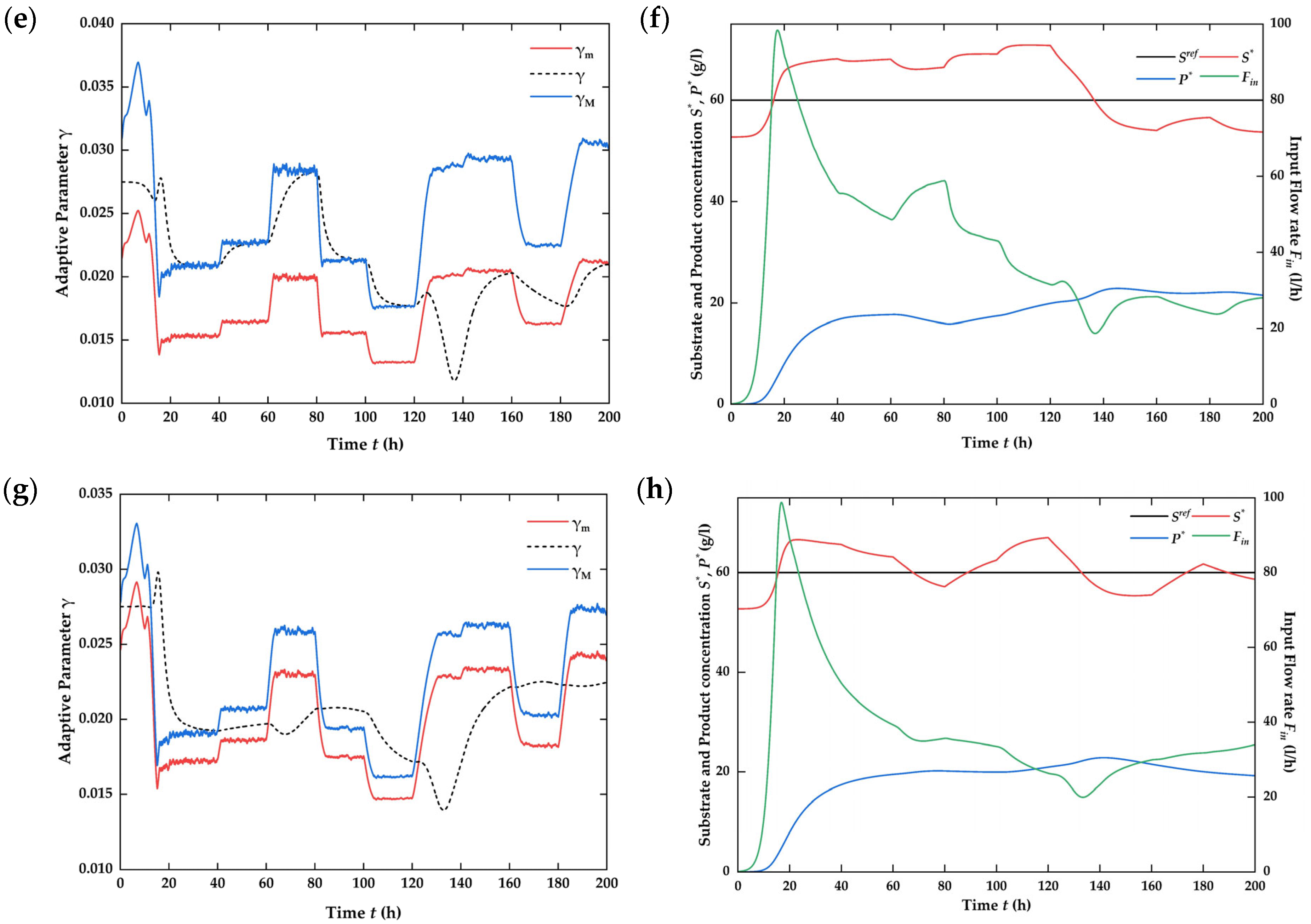
In the following, we consider the practical case that γm and γM are time-varying when inputs vary. As is shown in Figure 9c,d, γm and γM follow the trend of Sin estimation and when the scope between (γm, γM) is set as S(γref/Sin), γ reaches γM and follows the trend (Figure 9c), and results in S to increase and maintain a high substrate run-off (Figure 9d). We can narrow down the regime (γm, γM) to force S → Sref: Figure 9e,g are the adaptive parameters under 0.6 and 0.2 times S(γref/Sin), respectively, and the corresponding control results are shown in Figure 9f,h. The control becomes aggressive when the domain of γ narrows down. Note that the fermentation reaction is very slow, and it is probable that the delay in response to the broth changes might deteriorate the control performance in real-time practice; hence, our purpose is not to precisely maintain the values at their reference but to shift between different operation modes with the least possible substrate loss.
Second case scenario. To increase ethanol conversion and decrease substrate loss, the second scenario is carried out considering that the reference Sref has a decreasing evolution under piece-wise constant steps, where the domains of the adaptive parameters (γm, γM) are set as 0.2 times S(γref/Sin). As is shown in Figure 10a, the reference jumps at t = 50 h, 15 h, and 300 h directly correspond to the scope change in γm and γM; however, the adaptive law promises γ to vary continuously, which is advantageous for system sensitive to external interference.
One problem related to the economically viable control is the selection of optimal reference Sref. To make the system continuous and functional, batch/washout avoidance is essential; hence, we wish the control input Fin to be somewhat inert to changes. As is shown in Figure 10b, for the ladder form decrease of Sref at t ∈ (0, 300) h, Fin tends to decrease after a quick increase at the beginning. Though Sref =20 g/L is hard to reach, ethanol production continuous to increase. Here, we can expect an optimal S in this case of around 30 g/L, and the corresponding Fin decrease to about 11 L/h. Further increase Sref = 60 g/L and the results show that ethanol production decreases and Fin increases slowly, indicating that the adaptive control is capable of maintaining continuous production whilst keeping Fin at a low flowrate, so as to decrease substrate loss. To mention, the process shift from batch mode to continuous mode is critical for the fermentation process, and we have noticed a time during exists before the start-up operation in dilution rate, which allows for cell accumulation, and during this time interval, the system is in batch mode. In the following, we introduce experimental collected CER signals and tests on this control system to evaluate the start-up procedure.
4.4. Assessment of Process Improvement [41]
To appreciate how the implementation of the continuous strategy could potentially impact ethanol production goals over a long-term period, we compared the results of Figure 9g,h with a batch in terms of ethanol productivity, substrate conversion, and substrate loss. For a reactor with a working volume (V) of 105 L, the downtime between batches was estimated at 6.0 h and the batch results repeated the regression of Figure 5d, as is exhibited in Figure 11a. The simulation results in a ~200 h interval show that the averaged ethanol productivity for continuous fermentation reaches 0.669 g L−1 h−1, which is 19.7% higher than the batch mode with the same start-up condition.
To evaluate substrate utility, the substrate conversion ratio (dP/dS) and substrate loss are presented in Figure 11a; the average conversion ratio in continuous mode is 0.369, while batch mode could be YSP = 0.3989 because the substrate loss of batch fermentation is very small. However, the substrate loss of continuous fermentation is substantial, for the current case where Sref is set as 60 g/L, the average outlet reaches 60.78 g/L. To mention, the configuration exhibited in Figure 3 is an effective solution to enhance substrate utility.
5. Conclusions
In this paper, a mathematical model for ethanol fermentation is proposed and validated with experimental data. Then, an innovative global stabilizing control scheme is developed and applied for continuous ethanol production that is started from batch mode. To address the problem of fermentation state monitoring, observer-based estimation strategies are developed, and for the estimation of unknown inputs, the technique of a higher-order sliding mode observer is adopted. Despite being in harsh, realistic operating conditions (unknown input substrate concentration, time-varying and uncertain kinetics, noisy measurements), the adaptive control structure behaved well, and the control achieves a 19.7% increase in volumetric productivity. The reported simulation results are encouraging, and the proposed control structure can be adapted to other types of fermentation processes.
Author Contributions
All authors contributed to the study conception and design. Material preparation, data collection, and analysis were performed by Y.Q. and C.Z. The first draft of the manuscript was written by Y.Q., and both authors commented on previous versions of the manuscript. All authors have read and agreed to the published version of the manuscript.
Funding
The authors gratefully acknowledge the following institutions for their support: Yunnan Major Scientific and Technological Projects (Grant No. 202202AG050001); Yunnan basic research project (Grant No. 202001AU070048).
Data Availability Statement
All data generated or analyzed during this study are included in this published article.
Conflicts of Interest
The authors declare that they have no conflicts of interest.
References
- Gonçalves, F.; Perna, R.; Lopes, E.; Maciel, R.; Tovar, L.; Lopes, M. Strategies to improve the environmental efficiency and the profitability of sugarcane mills. Biomass Bioenerg. 2021, 148, 106052. [Google Scholar] [CrossRef]
- Bilal, M.; Wang, Z.; Cui, J.D.; Ferreira, L.F.R.; Bharagava, R.N.; Iqbal, H.M.N. Environmental impact of lignocellulosic wastes and their effective exploitation as smart carriers–A drive towards greener and eco-friendlier biocatalytic systems. Sci. Total Environ. 2020, 722, 137903. [Google Scholar] [CrossRef] [PubMed]
- Deng, W.P.; Feng, Y.C.; Fu, J.; Guo, H.W.; Guo, Y.; Han, B.X.; Jiang, Z.C.; Liu, H.C.; Nguyen, P.T.T.; Ren, P.N.; et al. Catalytic conversion of lignocellulosic biomass into chemicals and fuels. Green Energy Environ. 2023, 8, 10–114. [Google Scholar] [CrossRef]
- Daugulis, A.J.; McLellan, P.J.; Li, J. Experimental investigation and modeling of oscillatory behavior in the continuous culture of Zymomonas mobilis. Biotechnol. Bioeng. 1997, 56, 99–105. [Google Scholar] [CrossRef]
- Herrera, W.E.; Rivera, E.C.; Alvarez, L.A.; Tovar, L.P.; Rojas, S.T.; Yamakawa, C.K.; Bonomi, A.; Maciel, R. Modeling and control of a continuous ethanol fermentation using a mixture of enzymatic hydrolysate and molasses from sugarcane. In Proceedings of the 2nd International Conference on Biomass, Taormina, Italy, 19–22 June 2016. [Google Scholar]
- Quintero, O.L.; Amicarelli, A.A.; Scaglia, G.; di Sciascio, F. Control based on numerical methods and recursive Bayesian estimation in a continuous alcoholic fermentation process. BioResources 2009, 4, 1372–1395. [Google Scholar] [CrossRef]
- Blanco-Sanchez, P.; Taylor, D.; Cooper, S. IEA Bioenergy Task 33 UK Country Report; International Energy Agency Bioenergy: Paris, France, 2021. [Google Scholar]
- Skupin, P.; Laszczyk, P.; Goud, E.C.; Vooradi, R.; Ambati, S.R. Robust nonlinear model predictive control of cascade of fermenters with recycle for efficient bioethanol production. Comput. Chem. Eng. 2022, 160, 107735. [Google Scholar] [CrossRef]
- Das, S. Mathematical Modelling of Bioenergy Systems for Stability Analysis and Parametric Sensitivity. Ph.D. Thesis, UiT The Arctic University of Norway, Tromsø, Norway, 2021. [Google Scholar]
- Zhai, C.; Yang, C.X.; Na, J. Bifurcation Control on the Un-Linearizable Dynamic System via Washout Filters. Sensors 2022, 22, 9334. [Google Scholar] [CrossRef] [PubMed]
- Straathof, A.J.J. Modelling of end-product inhibition in fermentation. Biochem. Eng. J. 2023, 191, 108796. [Google Scholar] [CrossRef]
- Kurth, J.M.; Nobu, M.K.; Tamaki, H.; de Jonge, N.; Berger, S.; Jetten, M.S.M.; Yamamoto, K.; Mayumi, D.; Sakata, S.; Bai, L.P.; et al. Methanogenic archaea use a bacteria-like methyltransferase system to demethoxylate aromatic compounds. ISME J. 2021, 15, 3549–3565. [Google Scholar] [CrossRef] [PubMed]
- Tu, B.P.; Kudlicki, A.; Rowicka, M.; McKnight, S.L. Logic of the yeast metabolic cycle: Temporal compartmentalization of cellular processes. Science 2005, 310, 1152–1158. [Google Scholar] [CrossRef] [PubMed]
- Sriputorn, B.; Laopaiboon, P.; Phukoetphim, N.; Polsokchuak, N.; Butkun, K.; Laopaiboon, L. Enhancement of ethanol production efficiency in repeated-batch fermentation from sweet sorghum stem juice: Effect of initial sugar, nitrogen and aeration. Electron. J. Biotechnol. 2020, 46, 55–64. [Google Scholar] [CrossRef]
- Peng, P.; Lan, Y.; Liang, L.; Jia, L. Membranes for bioethanol production by pervaporation. Biotechnol. Biofuels 2021, 14, 10. [Google Scholar] [CrossRef] [PubMed]
- Chai, W.Y.; Teo, K.T.K.; Tan, M.K.; Tham, H.J. Fermentation Process Control and Optimization. Chem. Eng. Technol. 2022, 45, 1731–1747. [Google Scholar] [CrossRef]
- Chai, W.Y.; Teo, K.T.K.; Tan, M.K.; Tham, H.J. Model predictive control in fermentation process—A review. In Proceedings of the 2nd Energy Security and Chemical Engineering Congress, Gambang, Malaysia, 29 August 2022. [Google Scholar]
- Shen, Y.; Zhao, X.Q.; Ge, X.M.; Bai, F.W. Metabolic flux and cell cycle analysis indicating new mechanism underlying process oscillation in continuous ethanol fermentation with Saccharomyces cerevisiae under VHG conditions. Biotechnol. Adv. 2009, 27, 1118–1123. [Google Scholar] [CrossRef] [PubMed]
- Prasad, D.; Kumar, M.; Srivastav, A.; Singh, R.S. Modelling of Multiple Steady-state Behavior and Control of a Continuous Bioreactor. Indian J. Sci. Technol. 2019, 12, 140476. [Google Scholar] [CrossRef]
- Bai, F.W.; Zhao, X.Q. High gravity ethanol fermentations and yeast tolerance. In Microbial Stress Tolerance for Biofuels; Springer: Berlin/Heidelberg, Germany, 2011. [Google Scholar]
- Navarro-Tapia, E.; Nana, R.K.; Querol, A.; Pérez-Torrado, R. Ethanol cellular defense induce unfolded protein response in yeast. Front. Microbiol. 2016, 7, 189. [Google Scholar] [CrossRef] [PubMed]
- Lopez, P.C.; Feldman, H.; Mauricio-Iglesias, M.; Junicke, H.; Huusom, J.K.; Gernaey, K.V. Benchmarking real-time monitoring strategies for ethanol production from lignocellulosic biomass. Biomass Bioenerg. 2019, 127, 105296. [Google Scholar]
- Periyasamy, S.; Isabel, J.B.; Kavitha, S.; Karthik, V.; Mohamed, B.A.; Gizaw, D.G.; Sivashanmugam, P.; Aminabhavi, T.M. Recent advances in consolidated bioprocessing for conversion of lignocellulosic biomass into bioethanol—A review. Chem. Eng. J. 2022, 453, 139783. [Google Scholar] [CrossRef]
- Petre, E.; Selişteanu, D.; Roman, M. Advanced nonlinear control strategies for a fermentation bioreactor used for ethanol production. Bioresour. Technol. 2021, 328, 124836. [Google Scholar] [CrossRef] [PubMed]
- Ciesielski, A.; Grzywacz, R. Nonlinear analysis of cybernetic model for aerobic growth of Saccharomyces cerevisiae in a continuous stirred tank bioreactor. Static bifurcations. Biochem. Eng. J. 2019, 146, 88–96. [Google Scholar] [CrossRef]
- Perrier, M.; Dochain, D. Evaluation of control strategies for anaerobic digestion processes. Int. J. Adapt. Control. Signal Process. 1993, 7, 309–321. [Google Scholar] [CrossRef]
- Czyżniewski, M.; Łangowski, R. A robust sliding mode observer for non-linear uncertain biochemical systems. ISA Trans. 2022, 123, 25–45. [Google Scholar] [CrossRef]
- Petre, E.; Selişteanu, D.; Roman, M. Control schemes for a complex biorefinery plant for bioenergy and biobased products. Bioresour. Technol. 2020, 295, 122245. [Google Scholar] [CrossRef]
- Pachauri, N.; Rani, A.; Singh, V. Bioreactor temperature control using modified fractional order IMC-PID for ethanol production. Chem. Eng. Res. Des. 2017, 122, 97–112. [Google Scholar] [CrossRef]
- Pachauri, N.; Singh, V.; Rani, A. Two degrees-of-freedom fractional-order proportional–integral–derivative-based temperature control of fermentation process. J. Dyn. Syst. Meas. Control. 2018, 140, 071006. [Google Scholar] [CrossRef]
- Sun, S.Y.; Gresham, D. Cellular quiescence in budding yeast. Yeast 2021, 38, 12–29. [Google Scholar] [CrossRef] [PubMed]
- Oh, T.H.; Park, H.M.; Kim, J.W.; Lee, J.M. Integration of reinforcement learning and model predictive control to optimize semi-batch bioreactor. AICHE J. 2022, 68, e17658. [Google Scholar] [CrossRef]
- Pinto, A.S.S.; Pereira, S.C.; Ribeiro, M.P.A.; Farinas, C.S. Monitoring of the cellulosic ethanol fermentation process by near-infrared spectroscopy. Bioresour. Technol. 2016, 203, 334–340. [Google Scholar] [CrossRef] [PubMed]
- Tiernan, H.; Byrne, B.; Kazarian, S.G. ATR-FTIR spectroscopy and spectroscopic imaging for the analysis of biopharmaceuticals. Spectrochim. Acta Part A Mol. Biomol. Spectrosc. 2020, 241, 118636. [Google Scholar] [CrossRef] [PubMed]
- Bernard, P.; Andrieu, V.; Astolfi, D. Observer design for continuous-time dynamical systems. Annu. Rev. Control 2022, 53, 224–248. [Google Scholar] [CrossRef]
- Bayen, T.; Rapaport, A.; Tani, F.Z. Improvement of performances of the chemostat used for continuous biological water treatment with periodic controls. Automatica 2020, 121, 109199. [Google Scholar] [CrossRef]
- Wang, J.; Chae, M.; Beyene, D.; Sauvageau, D.; Bressler, D.C. Co-production of ethanol and cellulose nanocrystals through self-cycling fermentation of wood pulp hydrolysate. Bioresour. Technol. 2021, 330, 124969. [Google Scholar] [CrossRef] [PubMed]
- Kumar, M.; Prasad, D.; Giri, B.S.; Singh, R.S. Temperature control of fermentation bioreactor for ethanol production using IMC-PID controller. Biotechnol. Rep. 2019, 22, e00319. [Google Scholar] [CrossRef] [PubMed]
- Kurth, A.C.; Sawodny, O. Control of age-structured population dynamics with intra specific competition in context of bioreactors. Automatica 2023, 152, 110944. [Google Scholar] [CrossRef]
- De Battista, H.; Jamilis, M.; Garelli, F.; Picó, J. Global stabilisation of continuous bioreactors: Tools for analysis and design of feeding laws. Automatica 2018, 89, 340–348. [Google Scholar] [CrossRef]
- Grisolia, G.; Fino, D.; Lucia, U. Thermodynamic optimisation of the biofuel production based on mutualism. Energy Rep. 2020, 6, 1561–1571. [Google Scholar] [CrossRef]
Figure 1.
Schematic of the bioreactor equipped with a jacket.

Figure 2.
Diagram of the plant information.
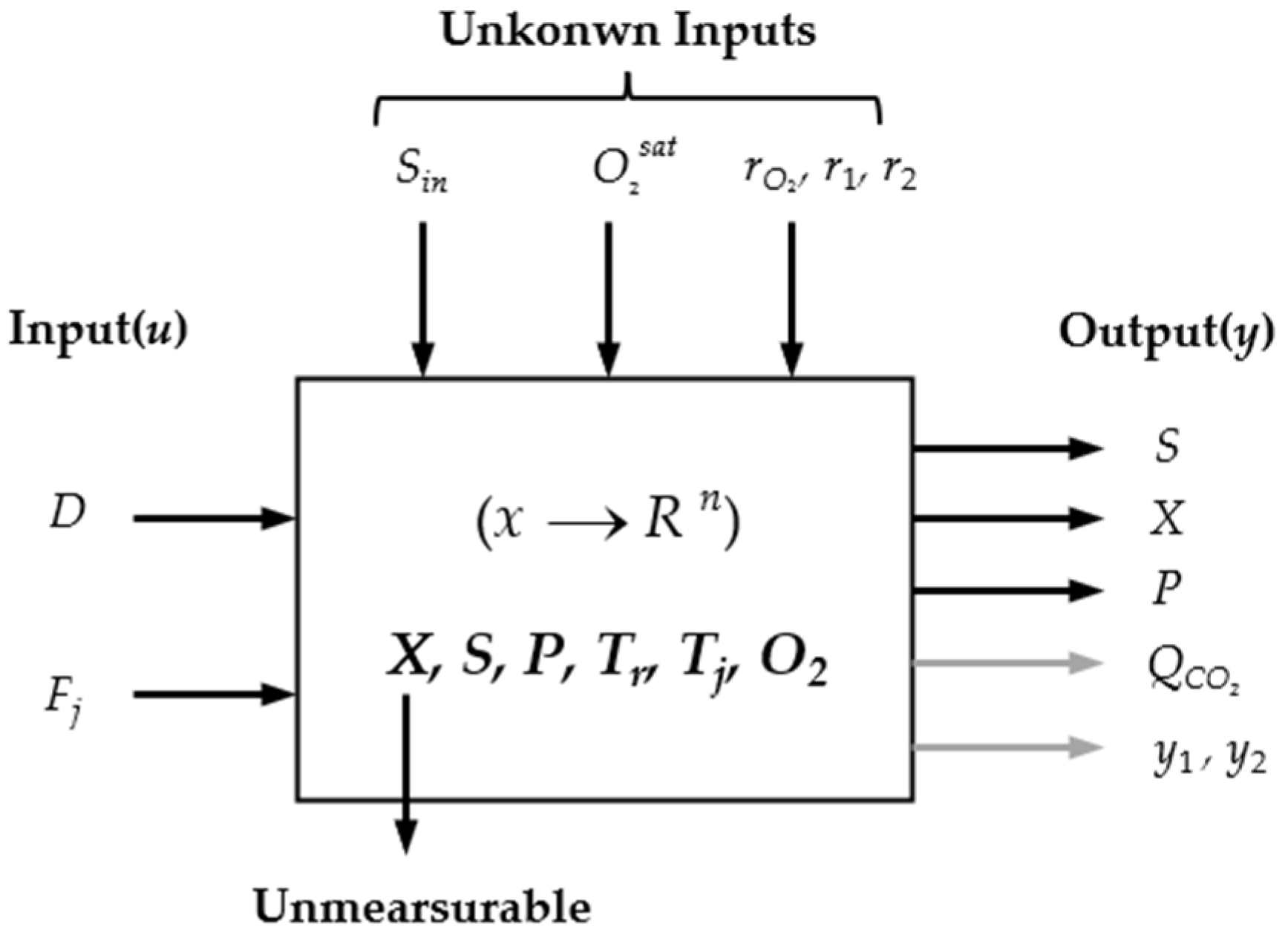
Figure 3.
Continuous ethanol fermentation flow-sheet and the corresponding state relations. Continuous fermentation with bio-reaction tanks in series, with partial reuse of the yeast cell separation; ethanol production efficiency increases, and the series of reactors form a gradient decline in substrate content loss.
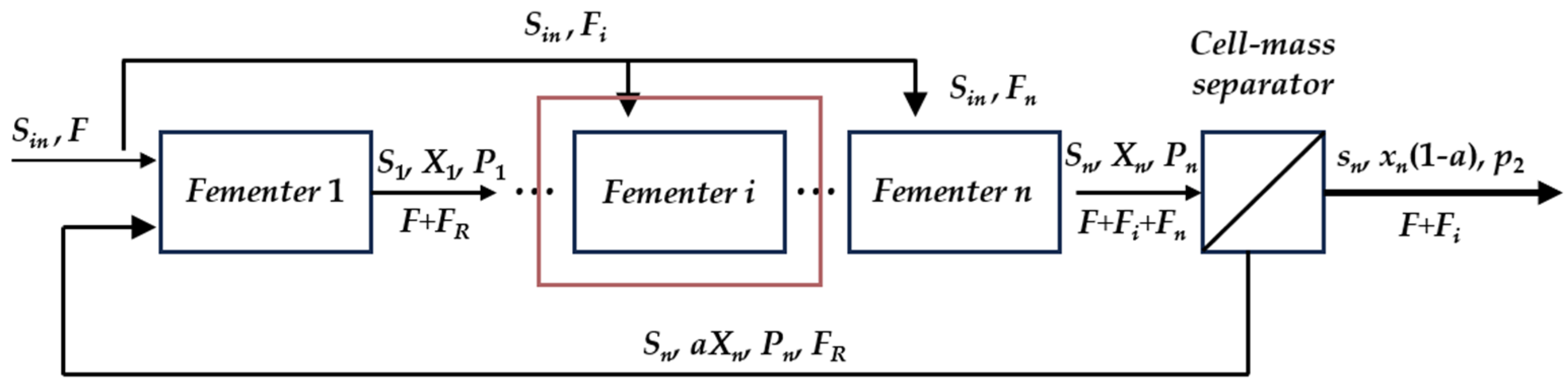
Figure 4.
Structure of the coupled control loops for ethanol fermentation.

Figure 5.
Experimental validation of the batch ethanol fermentation process. (a) Regression of YSP (0.3989) by experimental data of substrate concentration against the product ethanol; (b) Regression of YSX (0.105) by experimental data of substrate concentration against OD600; (c) Proportional relation of OD600 with the calculated biomass content, where the initial biomass is set as 0.01 by corrected inoculum size, and the biomass concentration is computed using literature data; (d) Fitting of the kinetics of Equation (33) using batch fermentation data.

Figure 6.
Numerical continuation of the ethanol fermentation process with varying parameters. (a) Ethanol production under varying dilution rate and input substrate concentration; (b) Influence of input substrate concentration on fermentation rate.
Figure 6.
Numerical continuation of the ethanol fermentation process with varying parameters. (a) Ethanol production under varying dilution rate and input substrate concentration; (b) Influence of input substrate concentration on fermentation rate.

Figure 7.
The split-ranging control schematic. When the actuators are off, “A” is in operation to remove the extra heat, and when the discharge/refill valves are open, “B” is in operation to remit the enthalpy loss.
Figure 7.
The split-ranging control schematic. When the actuators are off, “A” is in operation to remove the extra heat, and when the discharge/refill valves are open, “B” is in operation to remit the enthalpy loss.

Figure 8.
State estimation and temperature control through control law (43) with constant Fin = 26 l/h. (a) Estimation of X by observation of P, where ω1 = 0.5 and γ1 = 0.75. (b) Estimation of rO2 by observation of X, where ω3 = 0.5 and γ3 = 1.0. (c) Estimation of Sin by 2nd order SMO of ψ, where κ1 = 0.075, κ2 = 2.5, λψ = 2.5, λψ1 = 2.5, ω2 = −1, μ1 = 3.8, μ2 = 2.1, γ3 = 1.0. (d) | KP = 0.5, KI = 0, KD = 1.5, η2 = 0.5.
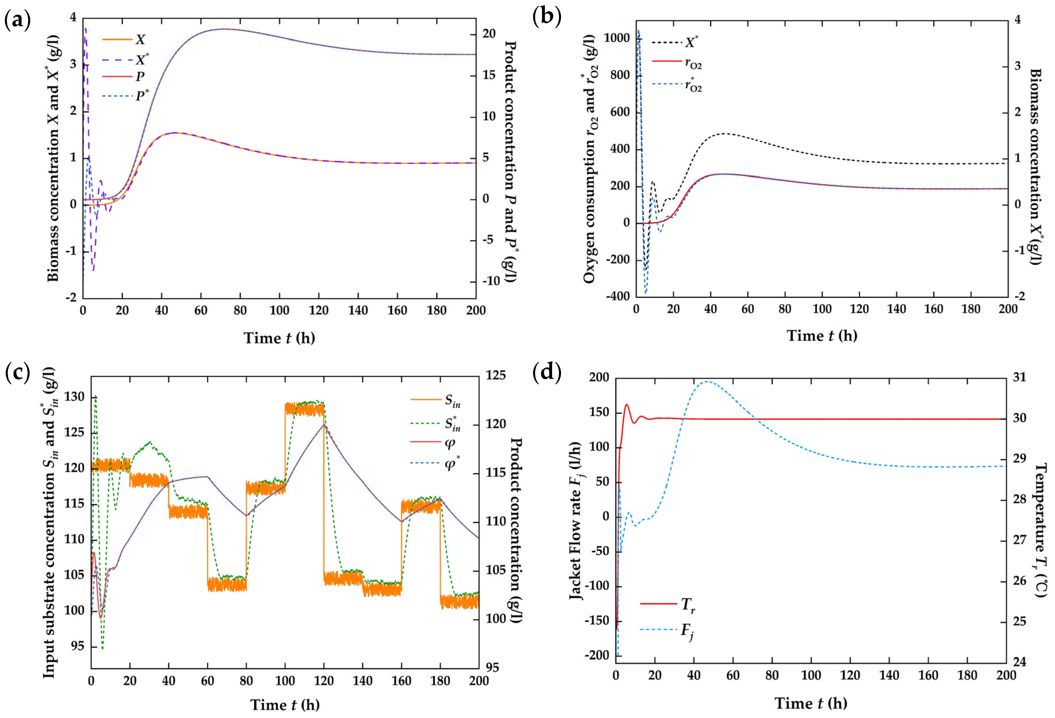
Figure 9.
Global stabilizing control through (17) with estimation, where Sref = 60 g/L and Trref = 30.0 °C. (a) Adaptive control with fixed parameters γm = 0.02 and γM = 0.03. (b) Control performance under K = 2.5 and fermenter states. (c) Control with adaptive parameters (γm, γM) = γref ± 0.5 × S(γref/Sin). (d) Control performance under K = 2.5 and fermenter states. (e) Control with adaptive parameters (γm, γM) = γref ± 0.3 × S(γref/Sin). (f) Control performance under K = 2.5 and fermenter states. (g) Control with adaptive parameters (γm, γM) = γref ± 0.1 × S(γref/Sin). (h) Control performance under K = 2.5 and fermenter states.
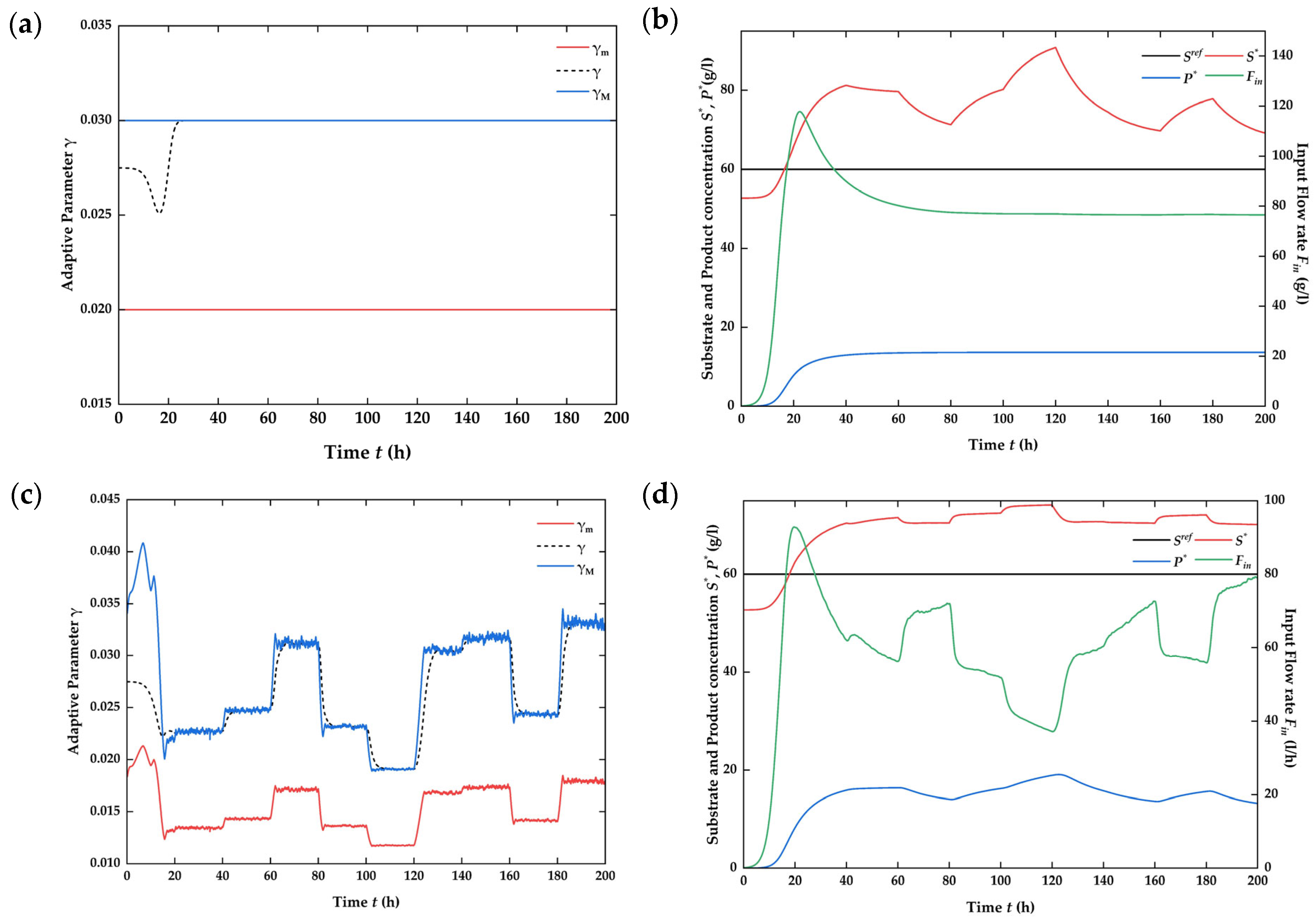

Figure 10.
Global stabilizing control with ladder form reference tracking, where Sref = 60 g/L and Trref = 30.0 °C. (a) Adaptive control with fixed parameters γm = γref − S(γref/Sin) and γM = γref + S(γref/Sin). (b) Control performance under K = 2.5 and fermenter states.
Figure 10.
Global stabilizing control with ladder form reference tracking, where Sref = 60 g/L and Trref = 30.0 °C. (a) Adaptive control with fixed parameters γm = γref − S(γref/Sin) and γM = γref + S(γref/Sin). (b) Control performance under K = 2.5 and fermenter states.

Figure 11.
Comparison of batch and continuous fermentation with the same start-up condition for 200 h interval. (a) Volumetric productivity for batch and continuous fermentation. (b) Substrate conversion ratio and substrate loss of the continuous mode.
Figure 11.
Comparison of batch and continuous fermentation with the same start-up condition for 200 h interval. (a) Volumetric productivity for batch and continuous fermentation. (b) Substrate conversion ratio and substrate loss of the continuous mode.


Table 1.
Process and kinetic parameters—description and values [38].
Table 1.
Process and kinetic parameters—description and values [38].
| Label | Description | Value | Label | Description | Value |
|---|---|---|---|---|---|
| A1 | Exponential factors in Arrhenius law | 1.57 × 10⁹ | MCa | Mol mass of Ca | 40 g/mol |
| A2 | Exponential factors in Arrhenius law | 4.20 × 1033 | MMg | Mol mass of Mg | 24 g/mol |
| AT | Heat transfer area | 1 m2 | MCl | Mol mass of Cl | 35.5 g/mol |
| Cheat,r | Heat capacity of culture medium | 4.18 J/g/°C | Mol mass of CO3 | 60 g/mol | |
| Cheat,j | Heat capacity of the cooling agent | 4.18 J/g/°C | MNaCl | Mol mass of NaCl | 58.5 g/mol |
| Ea1 | Activation energy | 55,000 J/mol | Mol mass of NaCO3 | 100 g/mol | |
| Ea2 | Activation energy | 220,000 J/mol | Mol mass of NaMgCl2 | 95.2 g/mol | |
| HOH | Specific ionic constant of OH | 0.941 | R | Universal gas constant | 8.31 J/mol/°C |
| HH | Specific ionic constant of H | −0.774 | YSP | Ethanol produced yield | 0.3989 g/g |
| HCO3 | Specific ionic constant of HCO3 | 0.485 | YSX | Biomass produced yield | 0.607 g/g |
| HCl | Specific ionic constant of Cl | 0.844 | V | Bioreactor volume | 1000 L |
| HMg | Specific ionic constant of Mg | −0.314 | Vj | Cooling jacket volume | 50 L |
| HCa | Specific ionic constant of Ca | −0.303 | O2 consumed rate | 0.970 mg/mg | |
| HNa | Specific ionic constant of Na | −0.55 | ΔHr | Aspiration heat | 518 kJ/mol |
| Ii | Ionic strengths | – | μO2 | O2 consumption rate | 0.5 h−1 |
| KLa0 | O2 mass-transfer coefficient | 38 h−1 | μP | Ethanol production rate | 1.79 h−1 |
| O2 consumption constant | 8.886 mg/L | ρj | Density of jacket liquid | 1000 g/L | |
| KE | Inhibition constant by ethanol | 0.139 g/L | ρr | Density of the medium | 1080 g/L |
| KE1 | Inhibition constant by ethanol | 0.07 g/L | mNaCl | Quantity of NaCl | 500 g |
| KS | Substrate constant for growth | 1.03 g/L | Quantity of CaCO3 | 100 g | |
| KS1 | Substrate constant for production | 1.68 g/L | Quantity of MgCl2 | 100 g | |
| KT | Heat transfer coefficient | 3.6 × 10⁵ J/h/m2/°C | MNa | Molecular mass of Na | 23 g/mol |
Disclaimer/Publisher’s Note: The statements, opinions and data contained in all publications are solely those of the individual author(s) and contributor(s) and not of MDPI and/or the editor(s). MDPI and/or the editor(s) disclaim responsibility for any injury to people or property resulting from any ideas, methods, instructions or products referred to in the content. |
© 2024 by the authors. Licensee MDPI, Basel, Switzerland. This article is an open access article distributed under the terms and conditions of the Creative Commons Attribution (CC BY) license (https://creativecommons.org/licenses/by/4.0/).
Share and Cite
MDPI and ACS Style
Qin, Y.; Zhai, C. Global Stabilizing Control of a Continuous Ethanol Fermentation Process Starting from Batch Mode Production. Processes 2024, 12, 819. https://doi.org/10.3390/pr12040819
AMA Style
Qin Y, Zhai C. Global Stabilizing Control of a Continuous Ethanol Fermentation Process Starting from Batch Mode Production. Processes. 2024; 12(4):819. https://doi.org/10.3390/pr12040819
Chicago/Turabian StyleQin, Yuxin, and Chi Zhai. 2024. "Global Stabilizing Control of a Continuous Ethanol Fermentation Process Starting from Batch Mode Production" Processes 12, no. 4: 819. https://doi.org/10.3390/pr12040819
Note that from the first issue of 2016, this journal uses article numbers instead of page numbers. See further details here.