A Linear Fit for Atomic Force Microscopy Nanoindentation Experiments on Soft Samples

Abstract

Atomic Force Microscopy (AFM) nanoindentation is a powerful technique for determining the mechanical properties of soft samples at the nanoscale. The Hertz model is typically used for data processing when employing spherical indenters for small indentation depths (h) compared to the radius of the tip (R). When dealing with larger indentation depths, Sneddon’s equations can be used instead. In such cases, the fitting procedure becomes more intricate. Nevertheless, as the h/R ratio increases, the force–indentation curves tend to become linear. In this paper the potential of using the linear segment of the curve (for h > R) to determine Young’s modulus is explored. Force–indentation data from mouse and human lung tissues were utilized, and Young’s modulus was calculated using both conventional and linear approximation methods. The linear approximation proved to be accurate in all cases. Gaussian functions were applied to the results obtained from both classic Sneddon’s equations and the simplified approach, resulting in identical distribution means. Moreover, the simplified approach was notably unaffected by contact point determination. The linear segment of the force–indentation curve in deep spherical indentations can accurately determine the Young’s modulus of soft materials at the nanoscale.

1. Introduction

Atomic Force Microscopy (AFM) has become a powerful tool for determining the mechanical properties of biological samples at the nanoscale due to its ability to work in near-physiological conditions [1,2]. Alongside its sub-nanometer resolution and pico-newton force sensitivity, AFM can identify changes at the molecular scale, detect compositional changes, and observe intercellular interactions within heterogeneous biological systems during the progression of diseases [3,4,5]. Numerous pioneering studies have explored the potential of employing AFM as a nano-diagnostic tool to establish impartial quantitative assessment criteria for monitoring pathological conditions, particularly in comparing healthy and pathological specimens [6]. Nanoscopic structures, mechanical properties, and single-molecular events were observed directly in cells and tissues through minimally invasive surgical interventions [7].

Key applications of AFM in medicine are associated with the detection of cancer. Specifically, the mechanical properties of individual normal cells exhibit significant differences when compared to cancer cells [8,9,10,11,12,13,14,15,16,17]. Therefore, the stiffness of tumor cells, measured in terms of Young’s modulus, can serve as a diagnostic method to differentiate them from normal cells [8]. The applicability of AFM in cancer diagnosis has also been demonstrated through experiments on normal, benign, and cancerous tissues [18,19,20,21,22,23]. For example, Plodinec et al. conducted experiments on human breast tissues and demonstrated that normal and benign tissues exhibit a consistent distribution of stiffness (in terms of Young’s modulus), whereas malignant tissue is characterized by two distinguishable maxima [18]. It is significant to also note that AFM as a diagnostic tool is not restricted to cancer diagnosis. For example, AFM has been proven effective in detecting osteoarthritis [24,25] and Alzheimer’s disease [26,27,28,29], among others [30].

The mechanical properties of biological samples at the nanoscale for biomedical applications, such as disease diagnosis, are typically determined using the AFM nanoindentation method [30,31]. Various mathematical models have been employed to fit the force–indentation data, depending on the indentation rate and the indenter’s shape [32,33,34,35,36,37,38]. When testing soft biological materials at low indentation rates using spherical indenters, the Hertz model is usually used for data processing. In particular, the applied force (F) and the indentation depth (h) are related through the following equation [32]:

$$F=\frac{4}{3}\frac{E}{1-v^2 }{R}^{1/2}{h}^{3/2}$$

(1)

where E and v are the Young’s modulus and the Poisson’s ratio of the material, respectively, and R is the indenter’s radius. Equation (1) is valid for small indentation depths compared to the tip radius (h << R) [39]. For big h/R ratios, Sneddon’s equation can be used instead [40]:

$$F=\frac{E}{2\left(1-v^2\right)}\left[\left(r_c^2+R^2\right)ln\left(\frac{R+r_c}{R-r_c}\right)-2r_{c}R\right]$$

(2)

where $r_c$ is the contact radius [40]. The contact radius is related to the indentation depth by the equation below:

$$\mathit{ln}\left(\frac{R+r_c}{R-r_c}\right)=\frac{2h}{r_c}$$

(3)

Since $r_c$ is a function of the indentation depth, Equations (2) and (3) do not directly relate F and h. Therefore, a new equation was recently derived [40]:

$$F=\frac{2ER}{1-v^2}hQ$$

(4)

where

$$Q=\frac{2}{3}{c}_1{R}^{-1/2}{h}^{1/2}+\frac{1}{2}{c}_2{R}^{-1}h+\frac{1}{3}{c}_3{R}^{-2}{h}^2+\frac{1}{4}{c}_4{R}^{-3}{h}^3+\dots +\frac{1}{N}{c}_N{R}^{1-N}{h}^{N-1}$$

(5)

In Equation (5), c₁ = 1.01, c₂ = −0.07303, c₃ = −0.1357, c₄ = 0.03598, c₅ = −0.004024 and c₆ = 0.0001653. To determine higher values of the c-coefficients (i.e., c₆ to c_N, where $N\to \infty$), refer to [40]. Equation (4) can be also written as follows for simplicity:

$$F=2E^{*}RhQ$$

(6)

where $E^{*}=E/(1-v^2)$ represents the sample’s reduced modulus. For $h>R$, the $F=f\left(h\right)$ curve tends to be linear [40]. In Figure 1a, the $\frac{F}{2E^{*}{R}^2}=f\left(\frac{h}{R}\right)$ data are presented in the domain $0<\frac{h}{R}<5$. For big h/R ratios, the force–indentation data tend to the following linear relationship [40]:

$$\frac{F}{2E^{*}{R}^2}=\frac{h}{R}-\frac{1}{2}$$

(7)

In Figure 1b,c, a spherical tip capable of indenting soft biological samples for h > R is presented. In Figure 1c,$h_c$ represents the contact depth, i.e., the depth at which contact is made between the indenter and the sample. For large indentation depths, $h_c$ approaches R. It is significant to note that Equation (7) has been theoretically proven but has not been experimentally tested up to today. Therefore, in this paper, we experimentally test the hypothesis that the force–indentation data are linear when using spherical indenters for large indentation depths.

Utilizing a simple linear approximation significantly simplifies the fitting process compared to fitting the data to Equations (2)–(5). Furthermore, it will be demonstrated that by determining the sample’s Young’s modulus using the linear portion of the force–indentation data, we significantly reduce errors arising from contact point misidentification. The proposed linear model is tested on lung tissues obtained from mice and humans, and the results are compared to those obtained using the classic Sneddon’s equations for data processing.

2. Materials and Methods

2.1. Tissue Samples from Mice

Normal lungs from 8–12-week-old C57BL/6 mice (The Cyprus Institute of Neurology & Genetics, Nicosia, Cyprus) were used. The in vivo experiments were conducted with bioethical approval from the Cyprus authorities (Veterinary services), under license number CY/EXP/PR.L03/2022. After sacrificing the mice, the lungs were excised. Post-excision, the tissues were immediately transferred to a PBS solution with a protease inhibitor cocktail. The tissue was kept at 4 °C until an experiment commenced (the samples were kept at 4 °C no longer than three days).

2.2. Tissue Samples from Human

The recruitment of the patients was performed at the Nicosia Lung Center by Dr. Zachariades. Informed consent was obtained from the patients who agreed to provide tissue for research purposes. All procedures and experimental protocols were approved by the Cyprus National Bioethics Committee (licenses ΕΕΒΚ/ΕΠ/2022/04). The human tissue samples (biopsies) were obtained through routine bronchoscopy performed for diagnostic and/or therapeutic purposes in newly diagnosed patients with pulmonary fibrosis. After the biopsy procedure, a portion of the collected tissue was provided to us, while the remaining tissue was appropriately handled by the clinical pulmonologist and histopathologist for histopathological examination.

2.3. Atomic Force Microscopy (AFM)

Atomic Force Microscopy (AFM) experiments were performed with a commercial AFM (5500 Keysight technologies, Santa Rosa, CA, USA) using the biosphere B150-FM tips (Nanotools, Munich, Germany) acquired from NanoAndMore (Wetzlar, Germany). The tip radius was 150 nm, and the sample’s Poisson’s ratio was assumed to be ν = 0.5 due to the high water content. The spring constant was calibrated using the thermal noise method, while sensitivity calibration (expressed as nanometers of cantilever deflection per volt signal from the laser detection system) was performed by acquiring force-versus-distance curves on a Petri dish, which serves as a pristine, rigid surface [41].

2.4. Contact Point Determination

When processing the force–indentation data using conventional methods (i.e., by fitting the appropriate contact mechanics models), a crucial step involves precisely determining the contact point between the tip and the sample. To ensure precision in results, the identification of the contact point was carried out using AtomicJ software version 2022 (https://sourceforge.net/projects/jrobust/, accessed on 23 March 2024) [42]. Each point on the curve is considered a trial contact point, where a polynomial is fitted to the precontact section, and an appropriate contact model is applied to the force–indentation data [42]. The point tested, which yields the lowest total sum of squares, is accepted as the contact point.

2.5. A linear Approximation for h > R

In this section, the simplified equations used for determining the Young’s modulus of the sample are introduced. For h > R, the contact stiffness S = dF/dh changes slightly with a low rate (as clearly shown in Figure 1a) and tends to the limit $S_{h\gg R}=2E^{*}R$. The average stiffness in the domain $h_{in}/R\le h/R\le h_f/R$ (where $h_{in}=R$ and $h_f=5R)$, can be calculated as follows:

$$S_{ave}=\frac{\Delta F}{\Delta h}=\frac{2ER}{1-v^2}\frac{h_f{Q}_f-h_{in}{Q}_{in}}{h_f-h_{in}}$$

(8)

For $h_{in}=R$ and $h_f=5R$, Equation (5) yields $Q_{in}=0.6$ and $Q_f=0.9,\mathrm{r}\mathrm{e}\mathrm{s}\mathrm{p}\mathrm{e}\mathrm{c}\mathrm{t}\mathrm{i}\mathrm{v}\mathrm{e}\mathrm{l}\mathrm{y}$. Therefore, Equation (8) results in the following:

$$S_{ave}=\frac{1.95ER}{1-v^2}$$

(9)

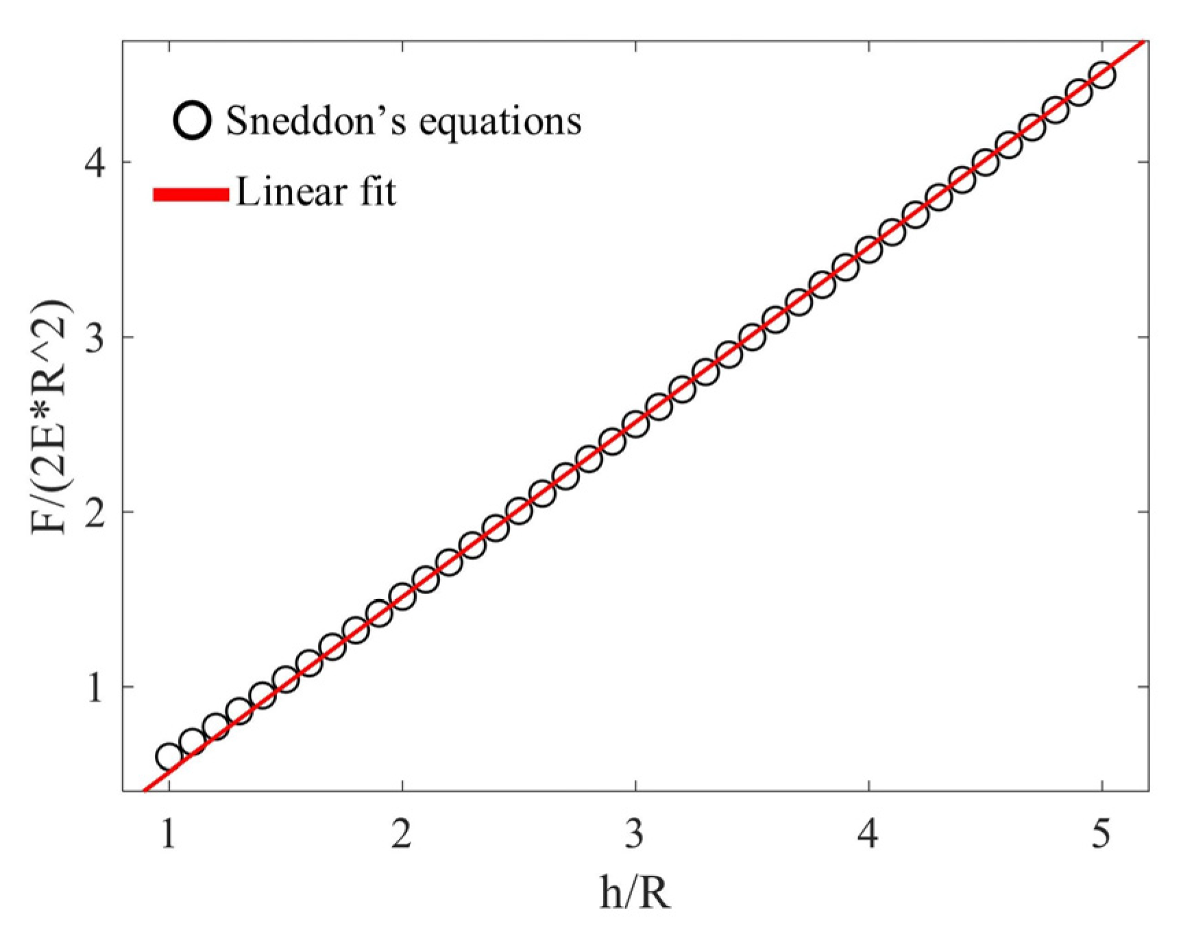
Equation (9) can be used for the Young’s modulus determination if $1<\frac{h_{max}}{R}<5$. In Figure 2, the $\frac{F}{2E^{*}{R}^2}=f\left(\frac{h}{R}\right)$ data using Equations (2)–(5) in the domain $1\le h/R\le 5$ are presented. The data were fitted to the following linear equation:

$$\frac{F}{2E^{*}{R}^2}=\lambda \frac{h}{R}+c$$

(10)

In Equation (10), $\lambda =1.95/2$ and $c=-0.4388$. The linear fit was accurate since the R-squared coefficient was close to 1 ($R_{s.c.}^2=0.9995$). This result is consistent with the case of big h/R ratios, since, in this case, the force–indentation curve tends to be linear as already mentioned (see Figure 1 a). For very large indentation depths (i.e., $h>5R$ ), it can be considered (using Equation (7)) that the average stiffness equals to

$$S_{ave}=\frac{2ER}{1-v^2}$$

(11)

In the following sections, Equations (9) and (11) are used to determine the Young’s modulus of lung tissues from mice and humans. The data in the domain h > R are fitted to a linear curve, and the slope of this curve is determined. Subsequently, if the maximum indentation depth is in the range $1<\frac{h_{max}}{R}<5$, Equation (9) can be employed. Otherwise (i.e., for h > 5R), Equation (11) is used. To examine the accuracy of the linear approximation, the percentage differences between the Young’s modulus calculated using the classic Equations (2)–(5) and (7) will be calculated as follows:

$$\pi \left(\%\right)=\frac{{|{\rm E}}_{acc.}-E_{lin}|}{E_{acc.}}100\%$$

(12)

2.6. Statistical Evaluation of the Results

To statistically evaluate the accuracy of the proposed method, Young’s modulus maps were constructed, and the distributions of Young’s modulus were plotted using both the Sneddon’s equations (Equations (2) and (3)) and the linear approximation (Equations (9) and (11)). The data were fitted in both cases to Gaussian curves:

$$f\left(E\right)=\frac{1}{\sigma \sqrt{2\pi }}{e}^{-\frac{1}{2}{\left(\frac{E-\mu }{\sigma }\right)}^2}$$

(13)

The mean values ${\mu }_{Sn} \mathrm{a}\mathrm{n}\mathrm{d} { \mu }_{lin}$ and the standard deviations ${\sigma }_{Sn} { \mathrm{a}\mathrm{n}\mathrm{d} \sigma }_{lin}$ using Sneddon’s equation and the linear approximation were recorded in each case. Using this approach, we tested the accuracy of the linear approximation when processing a large number of force curves. The Young’s modulus map creation and the Gaussian fittings were performed in Matlab R2022b (Mathworks, Natick, MA, USA).

3. Results

3.1. Force–Indentation Data on Murine Lung Tissues

Typical force–indentation data on lung tissue from mice are presented in Figure 3.

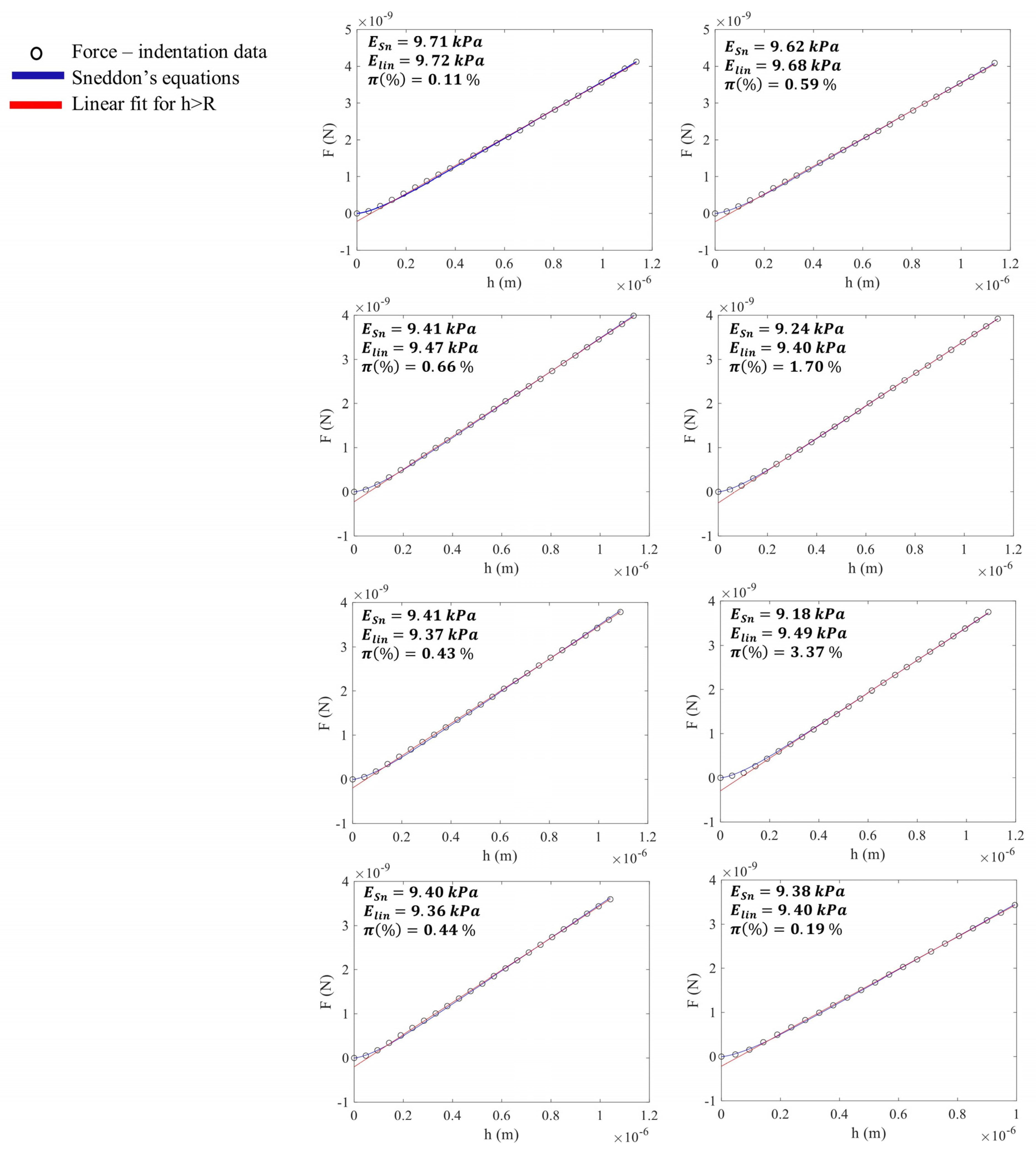
The data were first fitted to Equations (2) and (3) in the domain 0 ≤ h ≤ h_max. Subsequently, linear fitting was also performed on the data for h > R = 150 nm. The Young’s modulus values, calculated using Sneddon’s Equations (2) and (3), as well as the linear approximation (Equation (9)), are presented for comparison in eight characteristic curves (Figure 3). The percentage differences in Young’s modulus calculations are also shown. The differences are small in any case.

It is also important to highlight that the linear fit in any case was accurate (the R-squared coefficient resulted in $R_{s.c.}^2 \ge 0.9997$ in all cases). In addition, as shown in Figure 4a, an 8 × 8 Young’s modulus map on lung tissue from mice was obtained and the data were processed using the Sneddon’s equations (Equations (2) and (3)). The tested area was 10 μm × 10 μm. As shown in Figure 4b, the same data were processed using the linear approximation for h/R > 1. The Young’s modulus in Figure 4b was calculated using Equation (9). The percentage differences in Young’s modulus calculations are presented in Figure 4c. In Figure 4d, the $h_{max}/R$ ratios are also presented. For large $h_{max}/R$ values, the percentage difference between the Young’s modulus calculated using Sneddon’s approach and the linear approximation is small. As the $h_{max}/R$ ratio decreases, the percentage differences increase as expected (i.e., the linear approximation is accurate for deep indentations, as mentioned earlier). In Figure 4e,f, histograms and Gaussian fits of the Young’s modulus values are presented. Figure 4e corresponds to the classic Sneddon’s equations, while Figure 4f corresponds to the linear approximation. Lung tissue comprises various cell types, including epithelial cells, fibroblasts, and endothelial cells, as well as extracellular matrix components such as collagen and elastin, alongside air spaces. The mechanical properties can vary significantly among these components, resulting in a wide range of Young’s modulus values. This is the reason for the mechanical differences among different areas in Figure 4e,f. For the case of Figure 4e, the mean of the distribution is ${\mu }_{Sn}=9.68 \mathrm{k}\mathrm{P}\mathrm{a}$ and the standard deviation ${\sigma }_{Sn}=0.82 \mathrm{k}\mathrm{P}\mathrm{a}$. In addition, for the case of Figure 4f, ${\mu }_{lin}=9.69 kPa$ and the standard deviation ${\sigma }_{lin}=0.63 \mathrm{k}\mathrm{P}\mathrm{a}$. This is an important result, as despite deviations exceeding 10% in some individual measurements (i.e., for curves with low $h_{max}/R$ ratios), the mean of the Gaussian distribution is only slightly affected (approximately ~0.1%). Therefore, the linear approximation is a valuable simplified method for processing force curves.

3.2. Force–Indentation Data on Human Lung Tissues

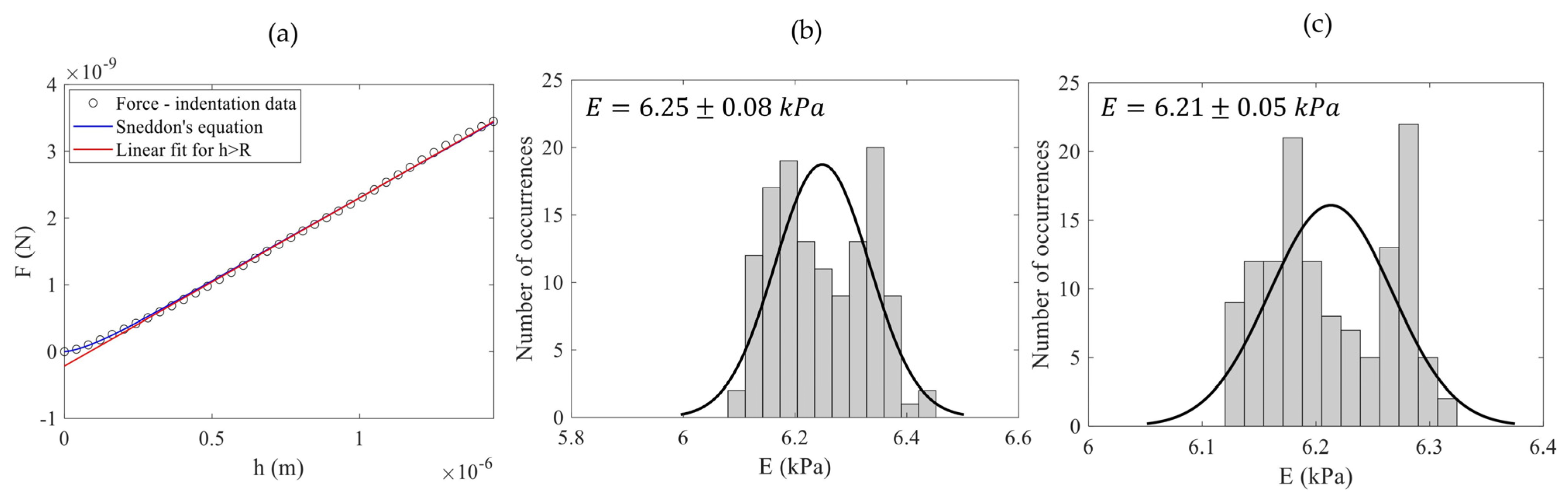
A typical force–indentation curve on human lung tissue is presented in Figure 5a. The force–indentation data were fitted to the Sneddon’s equations. In addition, linear fitting for h > R was also performed. The Young’s modulus calculated using the Sneddon’s equations resulted in $E_{Sn}=6.24 \mathrm{k}\mathrm{P}\mathrm{a}$, while using the linear approximation and Equation (11) (since $\frac{h}{R}>5$) resulted in $E_{lin}=6.30 \mathrm{k}\mathrm{P}\mathrm{a}$. The percentage difference was negligible (0.95%). In Figure 5b, the Young’s modulus values of 128 measurements are presented using the classic Sneddon’s equations.

The data were fitted to a Gaussian curve ($E_{Sn}=6.25\pm 0.08 \mathrm{k}\mathrm{P}\mathrm{a}$). As shown in Figure 5c, the same data were processed using the linear approximation and Equation (11). The mean of the distribution $\pm$ standard deviation values resulted in $E_{lin}=6.21\pm 0.05 \mathrm{k}\mathrm{P}\mathrm{a}$. The percentage difference between the means of the Gaussian distributions in Figure 5b,c was approximately 0.64%.

3.3. The Independence of the Contact Point Determination

It is important to emphasize that, unlike the conventional fitting process, the suggested approach is minimally impacted by the determination of the contact point between the AFM tip and the sample. When examining soft materials, determining the contact point presents a challenge because the cantilever’s deflection does not exhibit a sudden transition from one point to another [43,44]. For small indentation depths, accurately determining the contact point is crucial for assessing the material’s mechanical properties. For example, in Figure 6a, three potential contact points between the AFM tip and the sample are illustrated. Previous research has shown that misidentifying the location of the contact point by just 50 nm could lead to Young’s modulus values being incorrectly estimated by an order of magnitude [45,46]. Misidentifying the contact point by less than 50 nm results in inaccuracies in the material properties for small indentations. However, the error decreases asymptotically beyond 200 nm of indentation, eventually leading to a correct estimation of material stiffness [45]. On the other hand, if the contact point is missed by more than 100 nm, it becomes impossible to accurately estimate the true material properties [45].

However, these significant errors resulting from misidentifying the contact point occur primarily when utilizing the initial part of the force–indentation curve. When analyzing the linear portion of the force–indentation data, precise knowledge of the exact contact point position has minimal impact on determining Young’s modulus. Explaining why the above statement is reasonable is straightforward. In particular, the force–indentation data in most cases follow the general law below [43]:

$$F={\Lambda }_n{{\rm E}}^{*}{h}^n$$

(14)

where${\Lambda }_n$ is a function that depends on the indenter’s shape and dimensions (e.g., for parabolic indenters, ${\Lambda }_n=\frac{4}{3}{R}^{1/2}$, while for perfect conical indenters with opening angle $\theta$, ${\Lambda }_n=\frac{2}{\pi }\mathrm{t}\mathrm{a}\mathrm{n}\left(\theta \right)$) and $\mathrm{n}$ is a parameter that depends on the indenter’s shape (e.g., $n=3/2$ for parabolic and $n=2$ for conical indenters). In addition, the applied force (F) is related to the cantilever’s spring constant (k) and the cantilever’s deflection (δ) with the following trivial equation [43,47,48]:

$$F=k\left(\delta -{\delta }_0\right)$$

(15)

where ${\delta }_0$ represents the cantilever’s deflection at the contact point. In addition, the indentation depth (h) is defined as the difference between the displacement of the sample of interest (z) (which represents the soft sample’s displacement towards the AFM tip) and the displacement of a hard material unaffected by the indenter. The displacement of the hard material is equivalent to the deflection of the cantilever under the same applied force (Figure 6b,c) [43,47,48].

$$h=\left(z-z_0\right)-\left(\delta -{\delta }_0\right)$$

(16)

In Equation (16), $z_0$ represents the sample’s displacement at the contact point. By combining Equations (14)–(16) we conclude the following:

$$k\left(\delta -{\delta }_0\right)={\Lambda }_n{{\rm E}}^{*}{\left[\left(z-z_0\right)-\left(\delta -{\delta }_0\right)\right]}^n$$

(17)

However, for spherical indenters, the parameters ${\Lambda }_n, n$ also vary with the indentation depth, as can be inferred from Equations (4) and (5). In particular,

$${\Lambda }_n=2R\left(\frac{2}{3}{c}_1{R}^{-\frac{1}{2}}{h}^{\frac{3}{2}}+\frac{1}{2}{c}_2{R}^{-1}{h}^2+\frac{1}{3}{c}_3{R}^{-2}{h}^3+\dots +\frac{1}{N}{c}_N{R}^{1-N}{h}^N\right)$$

(18)

In addition, for small h/R ratios, $n\cong 3/2$ (as for the case of parabolic indenters), while for big h/R ratios, $n\cong 1$. Therefore, for big h/R ratios, ${\Lambda }_n\cong 2R$ and $n\cong 1$ (since, in this case, the projected contact area between the indenter and the sample is constant and the behavior is similar to the case of a flat punch [40]). Consequently, Equation (17) can be simplified as follows:

$${{\rm E}}^{*}=\frac{k\left(\delta -{\delta }_0\right) }{2R\left[\left(z-z_0\right)-\left(\delta -{\delta }_0\right)\right]}$$

(19)

Thus, $\delta -{\delta }_0=F/k$ and $z-z_0=F/k^{\prime }$ (where $k^{\prime }$ is a constant parameter that depends on the material’s properties and on the cantilever’s spring constant). As a result,

$$\left(z-z_0\right)-\left(\delta -{\delta }_0\right)=F\left(\frac{1}{k}-\frac{1}{k^{\prime }}\right)$$

(20)

By combining Equations (15) and (20) we conclude the following:

$$\left(z-z_0\right)-\left(\delta -{\delta }_0\right)=k\left(\delta -{\delta }_0\right)\left(\frac{1}{k}-\frac{1}{k^{\prime }}\right)\Rightarrow z-z_0=\left[1+k\left(\frac{1}{k}-\frac{1}{k^{\prime }}\right)\right]\left(\delta -{\delta }_0\right)$$

(21)

Hence, $z-z_0=c\left(\delta -{\delta }_0\right)$, where $c=1+k\left(\frac{1}{k}-\frac{1}{k^{\prime }}\right)$ is a constant dimensionless parameter that depends on the cantilever spring constant and the tested material properties. Therefore,

$${{\rm E}}^{*}=\frac{k}{2R(c-1)}$$

(22)

In soft materials, the parameter c should be larger compared to stiff materials, as a large displacement of the sample results in a small cantilever deflection. In the case of a very stiff sample, such as mica, that cannot be deformed by the AFM tip and where c = 1, Equation (22) is not applicable because it is impossible to determine the mechanical properties of a sample that is not being deformed by the indenter. Based on the analysis above, theoretically, the accuracy of calculating Young’s modulus depends primarily on the cantilever’s spring constant and the indenter’s radius, rather than on determining the contact point.

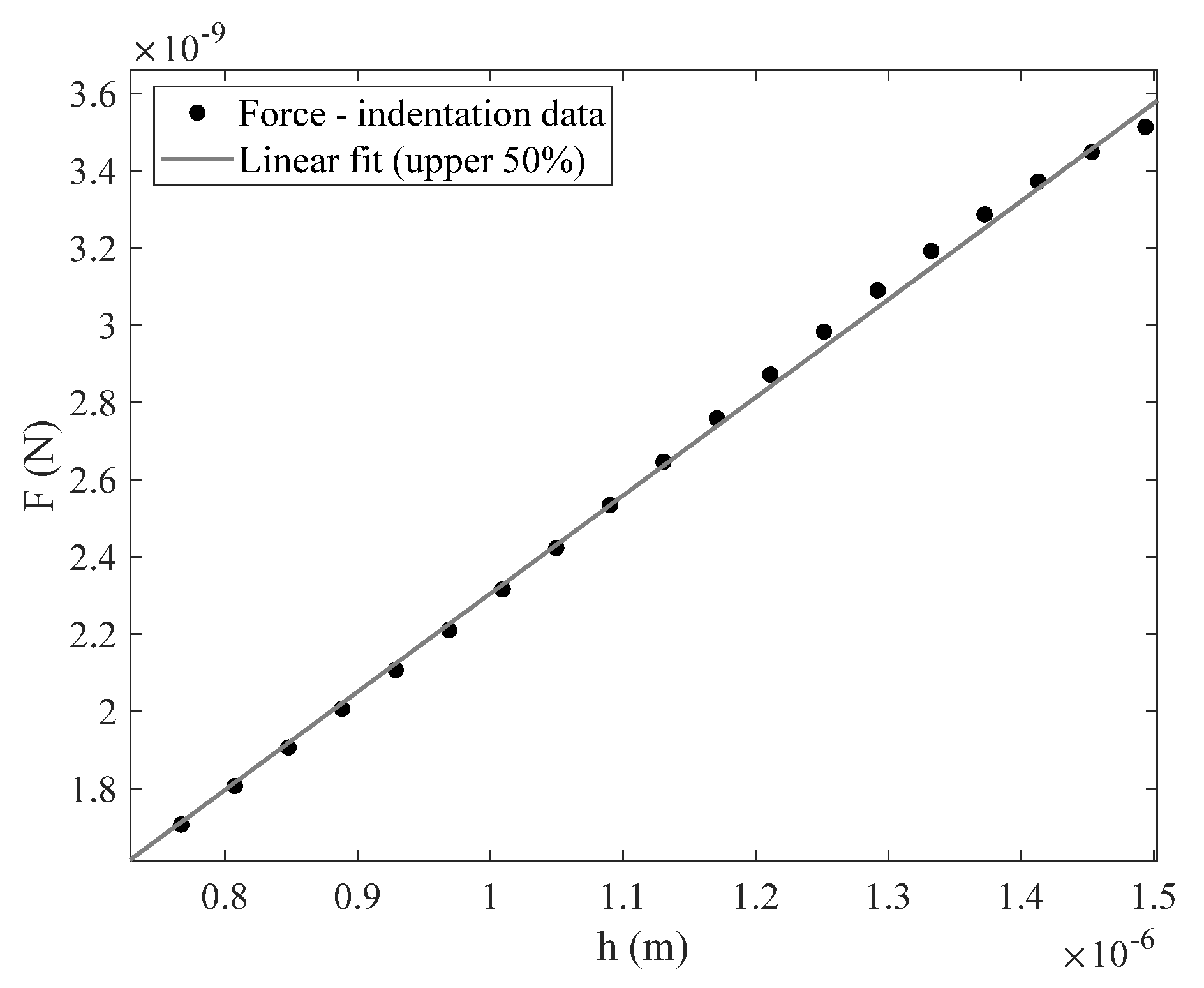
This represents a significant advantage of this approach compared to classic techniques. However, it is important to note that in practice, there is still a minor influence of the contact point even in this scenario. The reason is that the fitting process always depends on the number of points being used. More specifically, the force–indentation curves used in this paper were generated using a spherical indenter with a radius of R = 150nm. The maximum indentation depths ranged from 700 nm to 1400 nm (i.e., 4.7 < h_max/R < 9.3). Since the force–indentation data are approximately linear for h > R, one can simply perform linear fitting for this range. On the other hand, another approach may involve utilizing the upper 50% of the force–indentation data (or similar). The Young’s modulus will be similar in these two cases, but not identical. The exact position of the contact point influences the number of points used in the fitting process. For example, in Figure 7, linear fitting was performed on the upper 50% of the data presented in Figure 5a. The Young’s modulus was 6.35 kPa instead of 6.30 kPa. However, the difference is small. Therefore, the influence of the contact point determination is negligible when compared to the classic method.

3.4. Force–Calibration Process

The uncertainties in the determination of the deflection sensitivity and the cantilever’s spring constant are the main sources of error in AFM nanoindentation experiments [41,49,50,51]. The reason is that the applied force is given by the following equation [41,48,50,51]:

$$F=kaV$$

(23)

where k (in N/m) represents the spring constant of the cantilever (also known as its bending stiffness), α (in nm/V) denotes the deflection sensitivity that converts the cantilever’s deflection from volts to nanometers, and V stands for the measured deflection of the cantilever in volts. These three parameters— k, α, and V—constitute the primary components that the AFM employs for force spectroscopy. It is significant to note that errors in the deflection sensitivity calculation can lead to extreme errors in Young’s modulus (up to 50%) [48,50,51].

However, it is also significant to pinpoint that the results in this paper are not affected by these errors. The reason is that the values of k and $a$ were initially used to create the force–indentation curves. Subsequently, we used these curves to determine the Young’s modulus using two different methods. The first method involves a conventional fitting to Sneddon’s equations, while the second method employs an approximate approach based on a linear fit for $\frac{h_{max}}{R}>1$. In both cases, the force values were exactly the same. Thus, the percentage differences between the Young’s modulus as calculated by the two methods are not affected by these systematic errors. Consider, for example, arbitrary values for $k$ and $a.$ Equation (6) (i.e., Sneddon’s equations) can be written in the following form:

$$V=\frac{2E_{SN}^{*}}{ak}RhQ$$

(24)

In other words, consider the scenario where the vertical axis represents the cantilever’s deflection in volts, rather than being calibrated in Newtons using $k$ and $a$. In this case, the fitting parameter being calculated is

$$S_{SN}=\frac{2E_{SN}^{*}R}{ak}$$

(25)

In addition, if using Equation (11) we conclude

$$S_{linear}=\frac{2E_{linear}^{*}R}{ak}$$

(26)

Therefore,

$$\begin{gathered} \pi \left(\%\right)=\frac{|S_{SN}-S_{linear}|}{S_{SN}}100\%=\frac{|E_{SN}^{*}-E_{linear}^{*}|}{E_{SN}^{*}}100\%\Rightarrow \\ \pi \left(\%\right)=\frac{|{{\rm E}}_{SN}-{{\rm E}}_{linear}|}{{{\rm E}}_{SN}}100\% \end{gathered}$$

(27)

In conclusion, errors in force calibration significantly affect the Young’s modulus values in AFM nanoindentation experiments. However, in our case, the purpose was to introduce a new simplified method for data processing and compare it to classic techniques. The percentage differences of the Young’s modulus calculations between the classic and the newly proposed method are unaffected by the uncertainties induced in the force calibration procedure.

4. Discussion

In this paper, a new simplified method for processing force–indentation data when using spherical indenters for very large indentation depths has been presented. The idea is to use spherical indenters for h > R because, in this case, the force–indentation data tends to be linear, and therefore, the fitting procedure becomes an elementary process. Additionally, when using this approach, the influence of the contact point determination on the results becomes negligible. The physical significance behind the linear relationship between F and h data is revealed by the general force indentation equation [33]:

$$S=\frac{dF}{dh}=2r_c{E}^{*}$$

(28)

The contact radius $r_c$ is related to the indenter’s radius $R$ using the following equation (in the domain $0\le h/R\le 5$) [40]:

$$\frac{r_c}{R}=c_1{\left(\frac{h}{R}\right)}^{1/2}+c_2\frac{h}{R}+c_3{\left(\frac{h}{R}\right)}^2+c_4{\left(\frac{h}{R}\right)}^3+c_5{\left(\frac{h}{R}\right)}^4+c_6{\left(\frac{h}{R}\right)}^5$$

(29)

It can be easily shown that as the indentation depth increases, the ratio $r_c/R$ approaches 1. In this case, the contact stiffness tends to be constant $(S\to 2R{E}^{*})$ [40]. For example, for $\frac{h}{R}=3$, $\frac{r_c}{R}=0.9947$, while for $\frac{h}{R}=5$, $\frac{r_c}{R}=0.9998$. Therefore, when the projected area between the indenter and the sample tends in a constant value, the force indentation data tend to be linear. This is a significant observation that significantly simplifies the data processing in AFM nanoindentation experiments. It is also noteworthy that researchers in materials science seek simplified linear approximations when testing materials. A characteristic example is related to force–indentation data in elastic–plastic contacts between the indenter and the sample. In particular, when testing hard materials, Doerner and Nix assumed that the contact area remains constant as the indenter is withdrawn, and the resulting unloading curve is linear [52]. Despite the more precise approximation of the unloading force–indentation data provided by Oliver and Pharr [53], the linear approximation of the upper part of the unloading curve has been extensively used in the past [24,25,54,55] because it significantly simplifies the analysis. In this paper, we provide a linear approximation for the loading force–indentation data when testing soft materials using spherical indenters. In addition, the major advantage of this method, apart from the provided simplicity, is that it is not significantly affected by the exact position of the contact point. When using spherical indenters, the force–indentation data follow the power law

$$F=constant·h^n$$

(30)

However, the exponent $n$ depends strongly on the $h/R$ ratio ($n=f\left(\frac{h}{R}\right)$). For small h/R ratios, $n\to 3/2$ [56,57] (parabolic behavior), while for large h/R ratios, $n\to 1$ (flat punch behavior) [40]. Therefore, the calculation of the Young’s modulus depends strongly on the contact point determination if using the initial segment of the force indentation data. The same strong dependence has been recorded in sphero-conical indentations in which the exponent $n$ varies in the domain $3/2\le n\le 2$ (one order of magnitude difference in Young’s modulus calculation for a contact point that was missed by 50 nm) [45,46]. On the contrary, if using the upper linear segment of the force–indentation data, the influence of the contact point determination in the Young’s modulus calculations is minimized. Hence, in this paper, a new, simplified, and accurate method for processing force–indentation data is proposed.

However, it is also important to note that there are limitations associated with large indentation depths, depending on the sample being tested. This is attributed to the potential for permanent deformation of the sample, known as elastic–plastic contact. Nevertheless, the maximum indentation depth values used in this paper are similar to those found in the literature, given the relatively small tip radius used. For example, Plodinec et al. conducted AFM indentation experiments on breast tissues (normal, benign, and cancerous), with maximum indentation depths ranging from 150 nm to 3000 nm, depending on the intrinsic mechanical differences within each biopsy [18]. Additionally, Tian et al. investigated the mechanical properties of liver cancer tissues. The corresponding indentation depths were in the range of 150 nm to 2000 nm, depending on the sample’s elasticity [20]. Furthermore, Pogoda et al. conducted AFM nanoindentation experiments on fibroblasts, with maximum indentation depths ranging from 200 nm to 1400 nm [58]. Moreover, Ding et al. conducted indentation experiments on cells using large indentation depths. In particular, the maximum indentation depths were approximately 1000 nm on skin melanoma cells, approximately 1500 nm on normal and cancerous breast cells, approximately 1600 nm on cutaneous melanoma cells, and approximately 1500 nm on fibroblasts [59]. In conclusion, large indentation depths are frequently utilized when testing the mechanical properties of soft biological samples.

It is also noteworthy that at high indentation rates, biological materials typically demonstrate viscoelastic behavior [35,60,61]. Significant mathematical efforts have previously been undertaken to ascertain the viscoelastic properties of soft materials. For example, in the case of a relatively small indentation of a flat surface with a spherical indenter of radius R, the time-dependent force relaxation can be expressed as follows [62]:

$$F\left(t\right)=\frac{8R^{1/2}}{3(1-v)}{\int }_{-\infty }^{t}G(t-\tau )\frac{d{h}^{\frac{3}{2}}(\tau )}{dt}d\tau$$

(31)

where $G\left(t\right)$ and $h\left(t\right)$ are the time-dependent relaxation modulus and indentation depth, respectively. In the particular scenario of a finite-step indentation, where the time derivative of h(t) remains zero both before and after the time interval required to perform the indentation with an amplitude of h, Equation (31) simplifies as follows [62,63]:

$$F\left(t\right)=\frac{8R^{\frac{1}{2}}{h}^{\frac{3}{2}}}{3\left(1-v\right)}G\left(t\right)$$

(32)

Hence, the time-dependent relaxation modulus G(t) of the viscoelastic material is directly correlated with the recorded force [60,61,62,63,64]. However, Equation (32) is applicable for small indentation depths compared to the tip radius (h < R/10) [62]. Therefore, as part of our future work, we aim to extend our analysis to encompass viscoelastic materials and large indentations (h > R).

5. Conclusions

In this paper, we tested the hypothesis that force–indentation data in spherical indentations tend to be linear for large h/R ratios. It was proven that the linear segment of the data provides an accurate yet simple method for determining the Young’s modulus of soft samples. Additionally, the major advantage of this approach is that it is not significantly affected by the exact position of the contact point. Therefore, this method may evolve into a gold-standard technique for testing soft materials at the nanoscale.

References

- Stylianou, A.; Kontomaris, S.V.; Yova, D. Assessing Collagen Nanoscale Thin Films Heterogeneity by AFM Multimode Imaging and Nanoindentation for NanoBioMedical Applications. Micro Nanosyst. 2014, 6, 95–102. [Google Scholar] [CrossRef]
- Kontomaris, S.V.; Stylianou, A. Atomic force microscopy for university students: Applications in biomaterials. Eur. J. Phys. 2017, 38, 033003. [Google Scholar] [CrossRef]
- Kiio, T.M.; Park, S. Nano-scientific Application of Atomic Force Microscopy in Pathology: From Molecules to Tissues. Int. J. Med. Sci. 2020, 17, 844–858. [Google Scholar] [CrossRef] [PubMed]
- Hinterdorfer, P.; Garcia-Parajo, M.F.; Dufrêne, Y.F. Single-Molecule Imaging of Cell Surfaces Using Near-Field Nanoscopy. Acc. Chem. Res. 2012, 45, 327–336. [Google Scholar] [CrossRef] [PubMed]
- Li, M.; Dang, D.; Liu, L.; Xi, N.; Wang, Y. Imaging and Force Recognition of Single Molecular Behaviors Using Atomic Force Microscopy. Sensors 2017, 17, 200. [Google Scholar] [CrossRef] [PubMed]
- Carvalho, F.A.; Connell, S.; Miltenberger-Miltenyi, G.; Pereira, S.V.; Tavares, A.; Ariëns, R.A.S.; Santos, N.C. Atomic Force Microscopy-Based Molecular Recognition of a Fibrinogen Receptor on Human Erythrocytes. ACS Nano 2010, 4, 4609–4620. [Google Scholar] [CrossRef] [PubMed]
- Rusu, M.; Dulebo, A.; Curaj, A.; Liehn, E.A. Ultra-rapid non-invasive clinical nano-diagnostic of inflammatory diseases. Discov. Rep. 2014, 1, e2. [Google Scholar] [CrossRef]
- Lekka, M.; Gil, D.; Pogoda, K.; Dulińska-Litewka, J.; Jach, R.; Gostek, J.; Klymenko, O.; Prauzner-Bechcicki, S.; Stachura, Z.; Wiltowska-Zuber, J.; et al. Cancer cell detection in tissue sections using AFM. Arch. Biochem. Biophys. 2012, 518, 151–156. [Google Scholar] [CrossRef] [PubMed]
- Goldmann, W.H.; Ezzell, R.M. Viscoelasticity in wild-type and vinculin-deficient (5.51) mouse F9 embryonic carcinoma cells examined by atomic force microscopy and rheology. Exp. Cell Res. 1996, 226, 234–237. [Google Scholar] [CrossRef] [PubMed]
- Goldmann, W.H.; Galneder, R.; Ludwig, M.; Xu, W.; Adamson, E.D.; Wang, N.; Ezzell, R.M. Differences in elasticity of vinculin-deficient F9 cells measured by magnetometry and atomic force microscopy. Exp. Cell Res. 1998, 239, 235–242. [Google Scholar] [PubMed]
- Lekka, M.; Laidler, P.; Gil, D.; Lekki, J.; Stachura, Z.; Hrynkiewicz, A.Z. Elasticity of normal and cancerous human bladder cells studied by scanning force microscopy. Eur. Biophys. J. 1999, 28, 312–316. [Google Scholar] [CrossRef] [PubMed]
- Lekka, M.; Lekki, J.; Marszałek, M.; Golonka, P.; Stachura, Z.; Cleff, B.; Hrynkiewicz, A.Z. Local elastic properties of cells studied by SFM. Appl. Surf. Sci. 1999, 141, 345–349. [Google Scholar] [CrossRef]
- Li, Q.S.; Lee, G.Y.H.; Ong, C.N.; Lim, C.T. AFM indentation study of breast cancer cells. Biochem. Biophys. Res. Commun. 2008, 374, 609–613. [Google Scholar] [CrossRef] [PubMed]
- Faria, E.C.; Ma, N.; Gazi, E.; Gardner, P.; Brown, M.; Clarke, N.W.; Snook, R.D. Measurement of elastic properties of prostate cancer cells using AFM. Analyst 2008, 133, 1498–1500. [Google Scholar] [CrossRef] [PubMed]
- Zhou, Z.L.; Ngan, A.H.W.; Tang, B.; Wang, A.X. Reliable measurement of elastic modulus of cells by nanoindentation in an atomic force microscope. J. Mech. Behav. Biomed. Mater. 2012, 8, 134–142. [Google Scholar] [CrossRef] [PubMed]
- Cross, S.E.; Jin, Y.-S.; Rao, J.; Gimzewski, J.K. Nanomechanical analysis of cells from cancer patients. Nat. Nano 2007, 2, 780–783. [Google Scholar] [CrossRef] [PubMed]
- Stylianou, A.; Gkretsi, V.; Stylianopoulos, T. Transforming Growth Factor-β modulates Pancreatic Cancer Associated Fibroblasts cell shape, stiffness and invasion. Biochim. Biophys. Acta 2018, 1862, 1537–1546. [Google Scholar] [CrossRef] [PubMed]
- Plodinec, M.; Loparic, M.; Monnier, C.A.; Obermann, E.C.; Zanetti-Dallenbach, R.; Oertle, P.; Hyotyla, J.T.; Aebi, U.; Bentires-Alj, M.; Lim, R.Y.H.; et al. The nanomechanical signature of breast cancer. Nat. Nanotechnol. 2012, 7, 757–765. [Google Scholar] [CrossRef] [PubMed]
- Ansardamavandi, A.; Tafazzoli-Shadpour, M.; Omidvar, R.; Jahanzad, I. Quantification of effects of cancer on elastic properties of breast tissue by Atomic Force Microscopy. J. Mech. Behav. Biomed. Mater. 2016, 60, 234–242. [Google Scholar] [CrossRef] [PubMed]
- Tian, M.; Li, Y.; Liu, W.; Jin, L.; Jiang, X.; Wang, X.; Ding, Z.; Peng, Y.; Zhou, J.; Fan, J.; et al. The nanomechanical signature of liver cancer tissues and its molecular origin. Nanoscale 2015, 7, 12998–13010. [Google Scholar] [CrossRef] [PubMed]
- Ciasca, G.; Sassun, T.E.; Minelli, E.; Antonelli, M.; Papi, M.; Santoro, A.; Giangaspero, F.; Delfini, R.; De Spirito, M. Nanomechanical signature of brain tumors. Nanoscale 2016, 8, 19629–19643. [Google Scholar] [CrossRef]
- Cui, Y.; Zhang, X.; You, K.; Guo, Y.; Liu, C.; Fang, X.; Geng, L. Nanomechanical Characteristics of Cervical Cancer and Cervical Intraepithelial Neoplasia Revealed by Atomic Force Microscopy. Med. Sci. Monit. 2017, 23, 4205–4213. [Google Scholar] [CrossRef] [PubMed]
- Minelli, E.; Ciasca, G.; Sassun, T.E.; Antonelli, M.; Palmieri, V.; Papi, M.; Maulucci, F.; Santoro, A.; Giangaspero, F.; Delfini, R.; et al. A fully-automated neural network analysis of AFM force-distance curves for cancer tissue diagnosis. Appl. Phys. Lett. 2017, 111, 143701. [Google Scholar] [CrossRef]
- Stolz, M.; Gottardi, R.; Raiteri, R.; Miot, S.; Martin, I.; Imer, R.; Staufer, U.; Raducanu, A.; Düggelin, M.; Baschong, W.; et al. Early detection of aging cartilage and osteoarthritis in mice and patient samples using atomic force microscopy. Nat. Nanotechnol. 2009, 4, 186–192. [Google Scholar] [CrossRef] [PubMed]
- Loparic, M.; Wirz, D.; Daniels, A.U.; Raiteri, R.; Vanlandingham, M.R.; Guex, G.; Martin, I.; Aebi, U.; Stolz, M. Micro- and nanomechanical analysis of articular cartilage by indentation-type atomic force microscopy: Validation with a gel-microfiber composite. Biophys. J. 2010, 98, 2731–2740. [Google Scholar] [CrossRef]
- Connelly, L.; Jang, H.; Teran Arce, F.; Capone, R.; Kotler, S.A.; Ramachandran, S.; Kagan, B.L.; Nussinov, R.; Lal, R. Atomic force microscopy and MD simulations reveal pore-like structures of all-d-enantiomer of Alzheimer’s β-amyloid peptide: Relevance to the ion channel mechanism of AD pathology. J. Phys. Chem. B 2012, 116, 1728–1735. [Google Scholar] [CrossRef] [PubMed]
- Hane, F.; Drolle, E.; Choi, Y.; Attwood, S.; Gaikwad, R.; Leonenko, Z. Atomic force microscopy and Kelvin probe force microscopy to study Alzheimer’s disease. Mater. Sci. Technol. Conf. Exhib. 2013, 18, 2817–2824. [Google Scholar]
- Song, S.; Ma, X.; Zhou, Y.; Xu, M.; Shuang, S.; Dong, C. Studies on the interaction between vanillin and β-amyloid protein via fluorescence spectroscopy and atomic force microscopy. Chem. Res. Chin. Univ. 2016, 32, 172–177. [Google Scholar] [CrossRef]
- Han, S.W.; Shin, H.K.; Adachi, T. Nanolithography of amyloid precursor protein cleavage with β-secretase by atomic force microscopy. J. Biomed. Nanotechnol. 2016, 12, 546–553. [Google Scholar] [CrossRef] [PubMed]
- Stylianou, A.; Kontomaris, S.V.; Alexandratou, E.; Grant, C. Atomic Force Microscopy on biological materials related to pathological conditions. Scanning 2019, 2019, 8452851. [Google Scholar] [CrossRef] [PubMed]
- Kontomaris, S.V.; Stylianou, A.; Malamou, A.; Nikita, K.S. An alternative approach for the Young’s modulus determination of biological samples regarding AFM indentation experiments. Mater. Res. Express 2019, 6, 025407. [Google Scholar] [CrossRef]
- Krieg, M.; Fläschner, G.; Alsteens, D.; Gaub, B.M.; Roos, W.H.; Wuite, G.J.L.; Gaub, H.E.; Gerber, C.; Dufrêne, Y.F.; Müller, D.J. Atomic force microscopy-based mechanobiology. Nat. Rev. Phys. 2019, 1, 41–57. [Google Scholar] [CrossRef]
- Kontomaris, S.V.; Stylianou, A.; Georgakopoulos, A.; Malamou, A. Is it mathematically correct to fit AFM data (obtained on biological materials) to equations arising from Hertzian mechanics? Micron 2023, 164, 103384. [Google Scholar] [CrossRef] [PubMed]
- Kontomaris, S.V.; Georgakopoulos, A.; Malamou, A.; Stylianou, A. The average Young’s modulus as a physical quantity for describing the depth-dependent mechanical properties of cells. Mech. Mater. 2021, 158, 103846. [Google Scholar] [CrossRef]
- Kontomaris, S.V.; Malamou, A.; Stylianou, A. The Hertzian theory in AFM nanoindentation experiments regarding biological samples: Overcoming limitations in data processing. Micron 2022, 155, 103228. [Google Scholar] [CrossRef] [PubMed]
- Chen, S.W.; Teulon, J.M.; Kaur, H.; Godon, C.; Pellequer, J.-L. Nano-structural stiffness measure for soft biomaterials of heterogeneous elasticity. Nanoscale Horiz. 2023, 8, 75–82. [Google Scholar] [CrossRef] [PubMed]
- Gavara, N. A beginner’s guide to atomic force microscopy probing for cell mechanics. Microsc. Res. Tech. 2017, 80, 75–84. [Google Scholar] [CrossRef] [PubMed]
- Yuan, W.; Ding, Y.; Wang, G. Universal contact stiffness of elastic solids covered with tensed membranes and its application in indentation tests of biological materials. Acta Biomater. 2023, 171, 202–208. [Google Scholar] [CrossRef] [PubMed]
- Koruk, H.; Pouliopoulos, A.N. Elasticity and Viscoelasticity Imaging Based on Small Particles Exposed to External Forces. Processes 2023, 11, 3402. [Google Scholar] [CrossRef]
- Kontomaris, S.V.; Malamou, A. A novel approximate method to calculate the force applied on an elastic half space by a rigid sphere. Eur. J. Phys. 2021, 42, 025010. [Google Scholar] [CrossRef]
- Stylianou, A.; Gkretsi, V.; Patrickios, C.S.; Stylianopoulos, T. Exploring the Nano-Surface of Collagenous and Other Fibrotic Tissues with AFM. In Fibrosis: Methods and Protocols; Rittié, L., Ed.; Springer: New York, NY, USA, 2017; pp. 453–489. [Google Scholar]
- Hermanowicz, P.; Sarna, M.; Burda, K.; Gabryś, H. AtomicJ: An open source software for analysis of force curves. Rev. Sci. Instrum. 2014, 85, 063703. [Google Scholar] [CrossRef]
- Lekka, M. Discrimination Between Normal and Cancerous Cells Using AFM. BioNanoScience 2016, 6, 65–80. [Google Scholar] [CrossRef] [PubMed]
- Hassan, E.A.; Heinz, W.F.; Antonik, M.D.; D’Costa, N.P.; Nageswaran, S.; Schoenenberger, C.A.; Hoh, J.H. Relative microelastic mapping of living cells by atomic force microscopy. Biophys. J. 1998, 74, 1564–1578. [Google Scholar] [CrossRef] [PubMed]
- Crick, S.L.; Yin, F.C. Assessing micromechanical properties of cells with atomic force microscopy: Importance of the contact point. Biomech. Model. Mechanobiol. 2007, 6, 199–210. [Google Scholar] [CrossRef] [PubMed]
- Gavara, N. Combined strategies for optimal detection of the contact point in AFM force-indentation curves obtained on thin samples and adherent cells. Sci. Rep. 2016, 6, 21267. [Google Scholar] [CrossRef] [PubMed]
- Kontomaris, S.V.; Stylianou, A.; Yova, D.; Politopoulos, K. Mechanical Properties of Collagen Fibrils on Thin Films by Atomic Force Microscopy Nanoindentation. In Proceedings of the 2012 IEEE 12th International Conference on Bioinformatics & Bioengineering (BIBE), Larnaca, Cyprus, 11–13 November 2012; pp. 608–613. [Google Scholar]
- Kámán, J.; Bonyár, A.; Huszánk, R. The Effect of Surface Inclination on AFM Force-Curve Calibration and Evaluation. In Proceedings of the 2018 41st International Spring Seminar on Electronics Technology (ISSE) Conference, Zlatibor, Serbia, 16–20 May 2018; pp. 1–4. [Google Scholar]
- Wenger, M.P.; Bozec, L.; Horton, M.A.; Mesquida, P. Mechanical properties of collagen fibrils. Biophys. J. 2007, 93, 1255–1263. [Google Scholar] [CrossRef] [PubMed]
- Schillers, H.; Rianna, C.; Schäpe, J.; Luque, T.; Doschke, H.; Wälte, M.; Uriarte, J.J.; Campillo, N.; Michanetzis, G.P.A.; Bobrowska, J.; et al. Standardized Nanomechanical Atomic Force Microscopy Procedure (SNAP) for Measuring Soft and Biological Samples. Sci. Rep. 2017, 7, 5117. [Google Scholar] [CrossRef] [PubMed]
- Kámán, J.; Huszánk, R.; Bonyár, A. Towards more reliable AFM force-curve evaluation: A method for spring constant selection, adaptive lever sensitivity calibration and fitting boundary identification. Micron 2019, 125, 102717. [Google Scholar] [CrossRef] [PubMed]
- Doerner, M.F.; Nix, W.D. A method for interpreting the data from depth-sensing indentation instruments. JMR 2011, 1, 601–609. [Google Scholar] [CrossRef]
- Oliver, W.C.; Pharr, G.M. Measurement of hardness and elastic modulus by instrumented indentation: Advances in understanding and refinements to methodology. JMR 2004, 19, 3–20. [Google Scholar] [CrossRef]
- Desrochers, J.; Amrein, M.A.; Matyas, J.R. Structural and functional changes of the articular surface in a post-traumatic model of early osteoarthritis measured by atomic force microscopy. J. Biomech. 2010, 43, 3091–3108. [Google Scholar] [CrossRef] [PubMed]
- Stolz, M.; Raiteri, R.; Daniels, A.U.; VanLandingham, M.R.; Baschong, W.; Aebi, U. Dynamic Elastic Modulus of Porcine Articular Cartilage Determined at Two Different Levels of Tissue Organization by Indentation-Type Atomic Force Microscopy. Biophys. J. 2004, 86, 3269–3283. [Google Scholar] [CrossRef] [PubMed]
- Koruk, H. Modelling Small and Large Displacements of a Sphere on an Elastic Half-Space Exposed to a Dynamic Force. Eur. J. Phys. 2021, 52, 055006. [Google Scholar] [CrossRef]
- Koruk, H. Development of an Improved Mathematical Model for the Dynamic Response of a Sphere Located at a Viscoelastic Medium Interface. Eur. J. Phys. 2022, 43, 25002. [Google Scholar] [CrossRef]
- Pogoda, K.; Jaczewska, J.; Wiltowska-Zuber, J.; Klymenko, O.; Zuber, K.; Fornal, M.; Lekka, M. Depth-sensing analysis of cytoskeleton organization based on AFM data. Eur. Biophys. J. 2011, 41, 79–87. [Google Scholar] [CrossRef] [PubMed]
- Ding, Y.; Wang, J.; Xu, G.-K.; Wang, G.-F. Are elastic moduli of biological cells depth dependent or not? Another explanation by a contact mechanics model with surface tension. Soft Matter 2018, 14, 7534–7541. [Google Scholar] [CrossRef]
- Darling, E.M.; Zauscher, S.; Block, J.A.; Guilak, F. A thin-layer model for viscoelastic, stress-relaxation testing of cells using atomic force microscopy: Do cell properties reflect metastatic potential? Biophys. J. 2007, 92, 1784–1791. [Google Scholar] [CrossRef] [PubMed]
- Carmichael, B.; Babahosseini, H.; Mahmoodi, S.N.; Agah, M. The fractional viscoelastic response of human breast tissue cells. Phys. Biol. 2015, 12, 046001. [Google Scholar] [CrossRef] [PubMed]
- Moreno-Guerra, J.A.; Romero-Sánchez, I.C.; Martinez-Borquez, A.; Tassieri, M.; Stiakakis, E.; Laurati, M. Model-Free Rheo-AFM Probes the Viscoelasticity of Tunable DNA Soft Colloids. Small 2019, 15, 1904136. [Google Scholar] [CrossRef] [PubMed]
- Chim, Y.H.; Mason, L.M.; Rath, N.; Olson, M.F.; Tassieri, M.; Yin, H. A one-step procedure to probe the viscoelastic properties of cells by Atomic Force Microscopy. Sci. Rep. 2018, 8, 14462. [Google Scholar] [CrossRef] [PubMed]
- Dimitriadis, E.K.; Horkay, F.; Maresca, J.; Kachar, B.; Chadwick, R.S. Determination of elastic moduli of thin layers of soft material using the atomic force microscope. Biophys. J. 2002, 82, 2798–2810. [Google Scholar] [CrossRef]
Figure 1.
Deep spherical indentations (h > R). (a) The data when using Equations (2)–(5) in the domain 0 < h/R < 5 and the linear behavior for big h/R ratios (Equation (7)). It can be assumed that the Young’s modulus can be accurately calculated by fitting the linear segment of the curve to Equation (7). (b) A spherical indenter which permits very deep indentations. A typical example is the biosphere B150-FM (nanotools) obtained by NanoAndMore. (c) A deep spherical indentation (h >> R). In this case, the contact radius is nearly identical to the tip radius (i.e., ).
Figure 2.
A linear approximation for deep spherical indentations. The data when using Equations (2)–(5) (mentioned as ‘Sneddon’s equations’ in the graph) and the linear approximation (Equation (10)) for 1 > h/R > 5 (mentioned as ‘Linear fit’). The fit is accurate since .
Figure 3.
Eight force–indentation curves on lung tissues from mice. The Young’s modulus was calculated in each case using Sneddon’s equations (Equations (2) and (3)) and the linear approximation (Equation (9)). The two methods provided similar results.
Figure 4.
Young’s modulus maps and statistics (data obtained on lung tissues from mice). (a) An 8 × 8 Young’s modulus map. The data were processed using Sneddon’s equations (area: 10 μm × 10 μm). (b) The same data processed using the linear approximation (Equation (9)). (c) The percentage differences between the results presented in (a,b). (d) The ratios for the measurements in (a,b). For small ratios, the error increases as shown in (c). (e,f) The Young’s modulus distributions and Gaussian fits for the measurements shown in figures (a) and (b), respectively.
Figure 5.
Measurements on human lung tissues. (a) A typical force–indentation curve (experimental data) on a human lung tissue. (b,c) The distributions of Young’s modulus values and Gaussian fits for 128 force–indentation curves obtained from human lung tissues when using Sneddon’s equation (b) and the linear approximation (c).
Figure 6.
Contact point determination and errors. (a) When testing a soft material, determining the contact point is challenging because there is no abrupt change in the cantilever’s deflection. Three possible contact points (A, B, C) are shown. (b) The indentation depth (h) results from the difference between the displacement of the sample and the cantilever’s deflection. The cantilever’s deflection is determined using a stiff material that is not deformed by the indenter (dashed lines in the graph). In this case, the curve is linear. The determination of the contact point is crucial for conventional methods since it affects the plot and the fitting process. When using spherical indenters for large indentation depths, the curve for the soft sample tends to be linear. (c) The curve becomes linear for deep spherical indentations. The Young’s modulus can be easily calculated using the slope of this curve multiplied by the cantilever’s spring constant and using Equations (9) and (11). In this case, the error resulting from the contact point misidentification is small.
Figure 7.
A linear fit was applied to the upper 50% of the force–indentation data (i.e., experimental data) presented in Figure 5a. The resulting Young’s modulus was 6.35 kPa. There is a small difference compared to the result derived using a linear fit for h > R (i.e., 6.30 kPa), as the fitting process is affected by the data points used.
Disclaimer/Publisher’s Note: The statements, opinions and data contained in all publications are solely those of the individual author(s) and contributor(s) and not of MDPI and/or the editor(s). MDPI and/or the editor(s) disclaim responsibility for any injury to people or property resulting from any ideas, methods, instructions or products referred to in the content. |
© 2024 by the authors. Licensee MDPI, Basel, Switzerland. This article is an open access article distributed under the terms and conditions of the Creative Commons Attribution (CC BY) license (https://creativecommons.org/licenses/by/4.0/).
Share and Cite
MDPI and ACS Style
Kontomaris, S.V.; Malamou, A.; Zachariades, A.; Stylianou, A. A Linear Fit for Atomic Force Microscopy Nanoindentation Experiments on Soft Samples. Processes 2024, 12, 843. https://doi.org/10.3390/pr12040843
AMA Style
Kontomaris SV, Malamou A, Zachariades A, Stylianou A. A Linear Fit for Atomic Force Microscopy Nanoindentation Experiments on Soft Samples. Processes. 2024; 12(4):843. https://doi.org/10.3390/pr12040843
Chicago/Turabian StyleKontomaris, Stylianos Vasileios, Anna Malamou, Andreas Zachariades, and Andreas Stylianou. 2024. "A Linear Fit for Atomic Force Microscopy Nanoindentation Experiments on Soft Samples" Processes 12, no. 4: 843. https://doi.org/10.3390/pr12040843
Note that from the first issue of 2016, this journal uses article numbers instead of page numbers. See further details here.