Efficient Control Discretization Based on Turnpike Theory for Dynamic Optimization


Process Systems Engineering Laboratory, Massachusetts Institute of Technology, 77 Massachusetts Avenue, Cambridge, MA 02139, USA
*
Author to whom correspondence should be addressed.
†
Current address: Aspen Technology, 20 Crosby Dr, Bedford, MA 01730, USA.
Processes 2017, 5(4), 85; https://doi.org/10.3390/pr5040085
Submission received: 12 November 2017
/
Revised: 8 December 2017
/
Accepted: 11 December 2017
/
Published: 18 December 2017
(This article belongs to the Special Issue Combined Scheduling and Control)
Abstract
:Dynamic optimization offers a great potential for maximizing performance of continuous processes from startup to shutdown by obtaining optimal trajectories for the control variables. However, numerical procedures for dynamic optimization can become prohibitively costly upon a sufficiently fine discretization of control trajectories, especially for large-scale dynamic process models. On the other hand, a coarse discretization of control trajectories is often incapable of representing the optimal solution, thereby leading to reduced performance. In this paper, a new control discretization approach for dynamic optimization of continuous processes is proposed. It builds upon turnpike theory in optimal control and exploits the solution structure for constructing the optimal trajectories and adaptively deciding the locations of the control discretization points. As a result, the proposed approach can potentially yield the same, or even improved, optimal solution with a coarser discretization than a conventional uniform discretization approach. It is shown via case studies that using the proposed approach can reduce the cost of dynamic optimization significantly, mainly due to introducing fewer optimization variables and cheaper sensitivity calculations during integration.

1. Introduction
The use of dynamic optimization for optimizing the performance of transient manufacturing processes has drawn much attention in recent years [1]. A typical dynamic optimization problem is to find optimal trajectories for process control variables, e.g., flowrates in a chemical process, so that a particular performance index is maximized subject to some process constraints. Numerical solution of dynamic optimization problems poses a number of difficulties. First, optimization over control trajectories gives rise to an infinite-dimensional optimization problem, which must be transformed to an approximate finite-dimensional one by discretizing control trajectories. In so-called indirect methods [2], control trajectories are discretized automatically along with the state variables as the integration routine solves a two-point boundary value problem. The resolution of the discretization depends on the error-control mechanism of the integrator. A disadvantage of indirect methods is the rather high level of expertise required to formulate the optimality conditions for problems of practical size and complexity. Moreover, it can be very difficult to solve the resulting boundary value problem, especially in the presence of constraints [2,3]. Direct methods, on the other hand, rely on a priori discretization of the control trajectories. Two main classes of direct methods are (i) the simultaneous method, where the dynamic model is also discretized, using e.g., collocation techniques and extra optimization variables [4], to arrive at a fully algebraic model and (ii) the sequential method, where the dynamic model is retained, and instead is resolved using numerical integration [5]. The focus in this work is on the sequential method that has shown capabilities for handling large-scale, stiff problems with high accuracy [6], arguably due to keeping the problem dimension relatively small [7] and the use of adaptive numerical integrators furnished with error control mechanisms.
The quality of the optimal solution is directly related to the quality of the control discretization, with a finer discretization generally offering an improved optimal solution. However, a finer discretization can lead to increased computational cost as a result of increased number of optimization variables, with too fine of a discretization also posing robustness issues [8]. For the sequential method, it also increases the cost of computing the sensitivity information by introducing extra sensitivity equations to the dynamic model. The integration of sensitivity equations can be a computationally dominant task despite the significant progress made so far regarding their efficient calculation (see [9,10,11]). This is especially true when the number of optimization variables is large, and can be a potentially limiting factor in applying dynamic optimization to large-scale processes.
A second difficulty with dynamic optimization arises from potentially severe nonlinearity caused by the embedded dynamic model. The nonlinearity can result in a highly nonconvex problem exhibiting many suboptimal local solutions. It is known that even small-scale dynamic systems can exhibit multiple suboptimal local solutions [12,13,14]. Unfortunately, a derivative-based optimization method can become trapped in any of these, which can lead to a suboptimal operation and loss of profit.
To deal with the issue of control discretization, nonuniform (i.e., not equally spaced) discretization techniques can be applied to reduce the effective number of discretization points needed. A simple way to do this is by considering the location of the discretization points as extra optimization variables. However, the extra optimization variables can cause additional nonconvexity, and thus suboptimal, local solutions, especially when the number of discretization points is fairly large. In the authors’ experience, this strategy often leads to convergence difficulties, thereby defeating the point of using a coarser discretization for faster convergence. More elegant nonuniform discretization techniques have been proposed, where the discretization points over the time horizon are distributed adaptively based on the behavior of the optimal trajectories. As a result, excessive discretization can be avoided while maintaining the quality of the solution. Srinivasan et al. [15] proposed a parsimonious discretization method for optimization of batch processes with control-affine dynamics. The method relied on analysis of the information from successive batch runs for approximating the structure of the control trajectory and improving the solution in the face of fixed parametric uncertainty. Binder et al. [16] presented an adaptive discretization strategy, in which the problem with a coarse discretization of the control trajectory is first solved. Then, using a wavelet analysis of the obtained optimal solution, together with the gradient information, the discretization is refined by eliminating discretization points that are deemed unnecessary and adding new points where necessary. The problem with the refined discretization is then solved to give an improved optimal solution, and the procedure is repeated for further improvements. In a subsequent variant, Schlegel et al. [17] used a pure wavelet analysis in the refinement step in order to make the strategy better suited for problems with path constraints. In addition, Schlegel and Marquardt [18] proposed another adaptive discretization strategy that explicitly incorporates the structure of the optimal control trajectory. Specifically, the solution with a coarse discretization is used to deduce the structure based on the active or inactive status of the bound and path constraints, and the deduced structure is used to refine the discretization. A combination of the two strategies is also possible as presented in [19]. Recently, Liu et al. [20] proposed an adaptive control discretization method, in which the discretization is refined by a particular slope analysis on the approximate optimal control trajectories. The dynamic optimization problem is solved again with the refined discretization, and the procedure is repeated until a stopping criterion based on the relative improvement of the objective function is met. The foregoing strategies can be applied to a wide class of dynamic optimization problems arising from both batch and continuous processes. Nonetheless, a major drawback of them is the need for repeated solution of the dynamic optimization problem in order to arrive at a satisfactory optimal solution. Depending on the case, this may be even more costly overall than a one-time optimization with a sufficiently fine discretization. In addition, the post-processing of results required for each refinement step would take additional time and expertise.
In this paper, a new approach to control discretization is presented. Similar to the above-mentioned strategies, it aims to create an adaptive discretization based on a deduction of the structure of the optimal trajectories. However, a different philosophy is used for this purpose. Specifically, the proposed approach is based on turnpike theory [21,22] in optimal control, which analyzes optimal control problems with respect to the structure of the optimal solution, i.e., optimal trajectories of the control and state variables. Turnpike theory has been used in the context of indirect methods in [23,24,25], where the structure of the optimal trajectories is exploited to approximate the resulting boundary-value problem by two initial-value problems corresponding to the initial and terminal segments of the time horizon. However, the focus in this work is on using turnpike theory for efficient control discretization in direct methods. Of particular interest is the input-state turnpike [26,27] structure, where both control and state optimal trajectories are composed of three phases: a transient phase at the beginning, followed by a non-transient phase that is close to the optimal steady state, followed by another transient phase at the end. This type of turnpike is called steady-state turnpike in this paper. The proposed approach exploits this structure to place the discretization points in an “optimal” way. To do so, an adaptive discretization strategy is built into the dynamic optimization formulation. In this way, the solution structure and locations of the discretization points are adjusted “dynamically” during the optimization iterations so that optimal trajectories with an adapted discretization scheme are obtained at convergence. Therefore, unlike the previous strategies, only one dynamic optimization problem is solved in the proposed approach, and no post-processing of the results is needed. Furthermore, the proposed approach helps deal with the issue of suboptimal solutions by potentially avoiding a number of such solutions whose trajectories do not conform to the turnpike structure. It is noted, however, that this approach is most suitable for optimization of transient continuous processes in which an approximate steady state may occur. It is not meant for optimization of batch or semi-batch processes, in which steady state is not possible.
The remainder of the paper is organized as follows. The problem statement along with some background on turnpike theory is presented in Section 2. The proposed control discretization approach is described in Section 3. Numerical case studies are performed in Section 4, which is followed by some conclusions in Section 5.
2. Problem Statement and Pertinent Background
The dynamic optimization problem under study can take a quite general form. For simplicity, however, a minimal formulation is considered below:
where and are vectors of control and state variables, respectively, with the state initial conditions; is the set of admissible controls defined as with bounds on ; and are vector functions of appropriate sizes representing the dynamic model and process constraints, respectively. Note also that equality constraints or path constraints can be included in the formulation with no impact on the validity of the ensuing developments.
The time-dependent control variables in Problem (1)–(4) give rise to an infinite-dimensional optimization problem. For a numerical solution, the problem dimension must be reduced to a finite one by discretizing over the time horizon. In this work, the popular piecewise constant discretization approach is used for this purpose. With the time horizon discretized over N (not necessarily uniform) epochs , ,...,, is approximated over each epoch by a constant parameter vector as , with and . The discontinuities in make the dynamic model (2) a continuous-discrete hybrid dynamic system [28]. The discrete behavior potentially occurs at times , (called event times). The dynamic system is said to switch from one mode to another at these times. The hybrid behavior can have implications regarding the differentiability of the dynamic system, and consequently that of the optimization problem, as discussed later.
The piecewise constant discretization reduces the optimization to one over the finite-dimensional parameter vector . However, the optimal solution of the approximated problem is generally inferior to that of the original one. To improve the solution, a finer discretization may be used by increasing the number of epochs N. The effect of increasing N, and thus the number of optimization variables, on the computational cost of the solution is twofold: (i) it increases the cost of parametric sensitivities that are calculated during solution of the dynamic model, as required by a gradient-based optimization solver; and (ii) it can increase the cost of optimization by requiring more iterations to be performed within the larger search space. In some cases, increasing N too much can also lead to robustness issues [8] and failure of the optimization solver.
The above computational concerns become even more important when dealing with large-scale models of real-life manufacturing processes. This motivates efficient control discretization strategies that can maintain the solution quality with a coarser discretization scheme. The new discretization approach presented in this paper relies on turnpike theory, which is reviewed in the following subsection.
Turnpike in Optimal Control
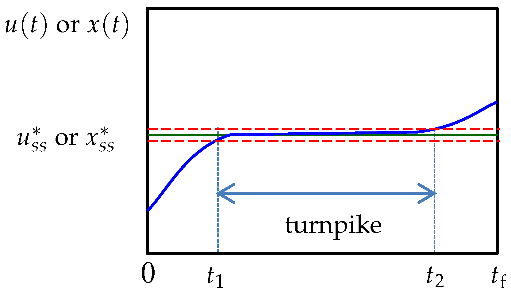
It appears that turnpike theory in optimal control was first discussed in the field of econometrics [22], and later gained attention in other fields including chemical processes [29]. The theory characterizes the structure of the solution of an optimal control problem by describing how the optimal control and state trajectories of a system evolve with time. It was initially investigated for optimal control problems with convex cost functions (in a minimization case). In particular, it was established that, given a time horizon , the time the optimal trajectories spend outside an -neighborhood of the optimal steady state is limited to two intervals and , where , with . The system is said to be in a transient phase in these intervals. The interesting point is that is independent of but only dependent on and the initial and final conditions of the system [30,31]. If the time horizon is long enough, i.e., , then a turnpike appears between and , and the turnpike trajectories lie in the -neighborhood of the optimal steady state. See Figure 1 for visualization of the concept. An appealing implication of turnpike theory is that an increase in will only stretch the duration of the turnpike, and has no effect on the duration and solution of the transient phases [32]. For relatively large , the optimal trajectories will traverse close to the optimal steady state for most of the time horizon, and the transient phases will be short in comparison.
The extension of turnpike theory to nonconvex problems has led to generalized definitions of the turnpike, in which it may no longer be a steady state, but a time-dependent trajectory [31,33]. Nonetheless, the interest in the present work is in a steady-state turnpike for generally nonconvex problems. Recently, it was shown in [27,34] that the steady-state turnpike still occurs if the convexity assumption is replaced by a dissipativity assumption. In particular, they present a notion of strict dissipativity, and prove that, if a dynamic system is strictly dissipative with respect to a reachable optimal steady state, then the optimal trajectories will have a turnpike at that steady state. Such a turnpike emerges in practice if the time horizon is sufficiently long. The equivalence of strict dissipativity and steady-state turnpike is a key result in optimal control and has applications in stability analysis of economic model predictive control [35,36].
3. Proposed Adaptive Control Discretization Approach
It is known that the emergence of a steady-state turnpike can be exploited in the numerical solution of optimal control problems, as noted in, e.g., [32,37], especially for problems with sufficiently long time horizons. In particular, the control trajectories need not be discretized over the entire horizon, but only over the intervals before and after the turnpike. If the turnpike interval is considerably long, this results in a coarser discretization and can reduce the computational load, as discussed earlier. However, the difficulty is that the duration of the turnpike and its location in the optimal trajectory are not known a priori. Therefore, it is not possible to adapt the discretization in advance based on the turnpike structure. To resolve this issue, this work considers embedding the tasks of approximating the turnpike structure and adaptive discretization into the dynamic optimization formulation. In this way, no pre- or post-processing for adjusting the discretization is needed. To this end, a first idea involves performing a nonuniform discretization where the duration of the epochs, i.e., and for are themselves optimization variables. To account for the turnpike, the parametrized controls on one of the intermediate epochs, e.g., the middle one, can be set to their optimal steady-state values. The following optimization problem will then result:
where gives the smallest integer not less than a. The optimal steady-state control is obtained from solving the following static optimization problem:
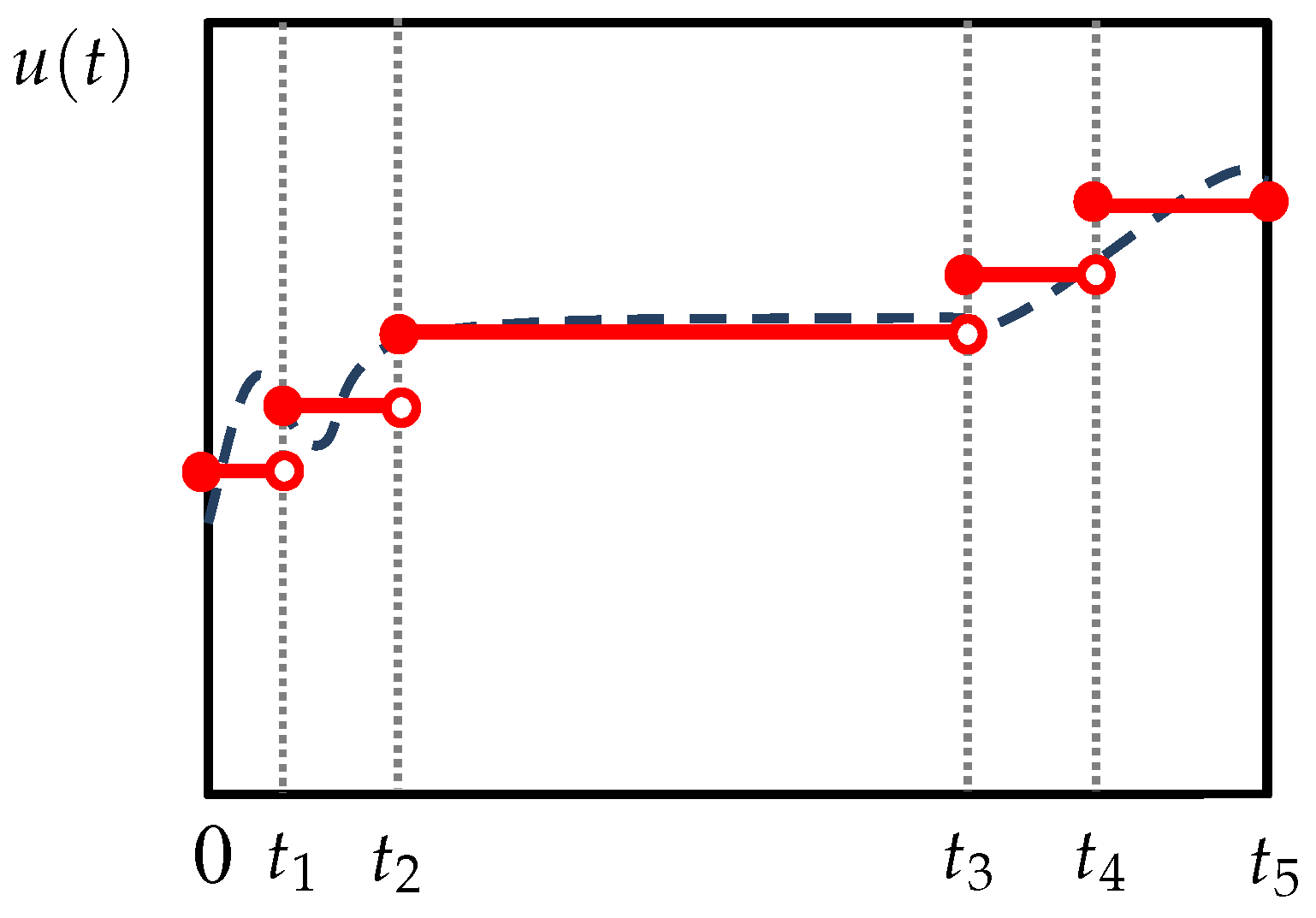
where are the bounds on . Problem (5)–(10) will generally prescribe a nonuniform discretization to minimize the objective function. Particularly, the optimizer can adjust so that only one epoch, here [,), is enough to represent the steady-state turnpike. The remaining epochs are automatically adjusted to cover the transient phases, where a finer discretization is needed. Problem (5)–(10) leads to a total of optimization variables. The nonuniform discretization is shown schematically in Figure 2, where the middle epoch is enlarged to cover the steady-state turnpike. In case no turnpike appears in the optimal solution, the corresponding to the turnpike can be simply pushed to zero by the optimizer. Therefore, the existence of a turnpike is not assumed and need not be verified in advance.
Note that the nonuniform discretization in Problem (5)–(10) results in a hybrid dynamic system with variable switching times . For numerical reasons, a change of variable is usually used to transform Problem (5)–(10) to one with fixed switching times [38,39]. More details about this transformation are deferred to the next subsection.
With the flexibility in the values of , it is expected that a lower N suffices to achieve the same optimal solution as in a uniform discretization. However, the addition of N optimization variables in the nonuniform discretization strategy can adversely affect the overall computational cost and offset the benefits gained by a coarser discretization. It could contribute to more nonconvexity and thus local suboptimal solutions. The alternative proposed in this work is a semi-uniform adaptive discretization approach, as described in the sequel.
Semi-Uniform Adaptive Control Discretization
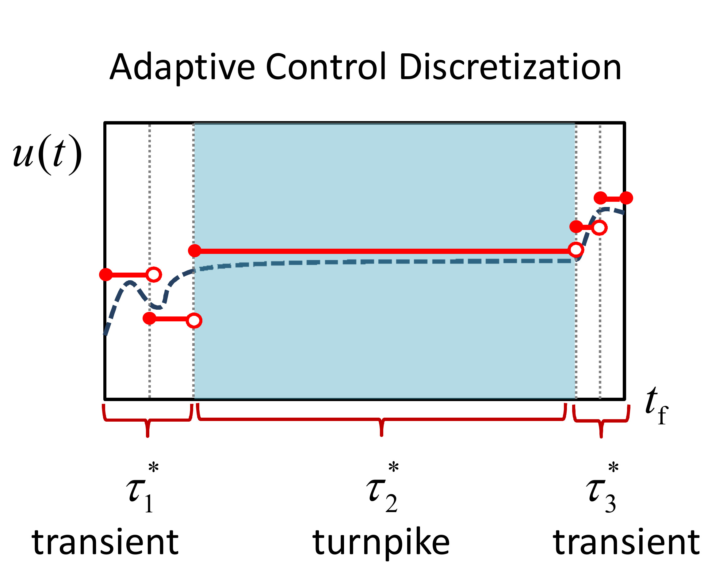
Here, a semi-uniform discretization approach for utilizing turnpike theory is proposed. The idea is to limit the use of nonuniform discretization where possible, while still being able to accommodate the variable durations of the steady-state turnpike and transient phases. To do so, the time horizon is split into the three phases prescribed by turnpike theory: two transient phases and a steady-state turnpike in between (see Figure 1). A uniform discretization is then applied on the transient phases, which connect to each other by one epoch representing the turnpike. The durations of these three phases are included as extra optimization variables. The approach is depicted in the left plot of Figure 3, where , , and denote the unknown durations of the first transient, turnpike, and second transient phases, respectively. Observe that the durations of the epochs in each particular phase are equal although they are generally not equal from one phase to another, hence a semi-uniform discretization. In addition, note that each of the transient phases can take a different resolution (i.e., number of epochs). This will allow for a more accurate solution of systems where, based on experience or engineering insights, one transient phase is deemed to be considerably longer or more severe than the other, thereby requiring a finer discretization. The semi-uniform discretization approximates as follows. Suppose the first transient phase (also called startup hereafter) is discretized into uniform epochs. Then, the control vector over is approximated as , , with and . In addition, suppose the second transient (also called shutdown hereafter) is discretized into uniform epochs. Then, the control vector over is approximated as , , with and . Notice that , represents the one-epoch discretization corresponding to the turnpike. With this discretization scheme, the proposed approach can be formulated through the following dynamic optimization problem:
where is the total number of epochs. The extra variables allow for the flexibility required to approximate the transient and turnpike phases well. Unlike the nonuniform formulation, however, the proposed formulation accommodates this flexibility by introducing only three extra optimization variables, regardless of the total number of epochs considered (the total number of optimization variables is in this formulation). Furthermore, if a steady-state turnpike does not appear for a particular system, the optimizer would push to zero. Therefore, the emergence of a turnpike need not be known a priori. However, this approach will best serve its purpose of reducing the computational cost if a turnpike exists and appears in the solution trajectories.
Similar to Problem (5)–(10), the proposed formulation results in a hybrid dynamic system with variable switching times. This is because the locations of discretization points depend on the variables . For example, the switch for from the first epoch to the second occurs at time according to the following statement:
Similarly, other switching times depend on and are not fixed. The computation of parametric sensitivities in a hybrid system where the switching times are a function of the parameters is involved and requires some assumptions for the system to ensure existence and uniqueness of the sensitivities [28]. Moreover, the parametric sensitivities are generally discontinuous over the switches [38], and additional computations are necessary to transfer the sensitivity values across the switches [28]. To avoid these numerical complications, the time transformation presented in [39,40] is used so that the switching times are fixed in the transformed formulation. In particular, the time horizon is transformed to a new time horizon using
in which
is a piecewise constant function on . With this transformation, Problem (13)–(18) is rewritten as:
where . Interestingly, each of the startup, turnpike, and shutdown phases has a duration of 1 in the domain, as shown in the right plot of Figure 3. Moreover, the switch from one phase to another now occurs at fixed times and . Accordingly, all the control switches are triggered at fixed times in the new time domain. This ensures existence and uniqueness of the parametric sensitivities and their continuity over the switches [28].
Despite the adaptive discretization strategy incorporated in Problem (22)–(27), the quality of the optimal solution can still depend on the resolutions set for the transient phases ( and ). If these resolutions are too coarse, the optimal solution may be compromised because the optimizer may have to adjust the s away from their true values, e.g., in order to keep the problem feasible. Even with an adequate resolution, it is possible that the s are under- or over-approximated by the local optimizer, thereby leading to an inferior solution. In some instances, it may be possible to avoid such a suboptimal solution by special modifications to the proposed formulation. In the next subsection, a variant formulation that can avoid a particular suboptimal scenario is presented.
A Variant Formulation
Figure 4 illustrates the suboptimal scenario that is dealt with by this variant formulation. The dashed lines show the optimal control trajectory that would be obtained ideally from no discretization. The left and right plots depict a suboptimal and an optimal solution, respectively, both obtained with the transient resolutions of . In the left plot, is under-approximated. As a result, part of the actual turnpike is deemed transient by the adaptive discretization scheme. This leads to unnecessarily using three epochs for the turnpike, leaving only one epoch to represent each transient phase. Observe, however, that the suboptimal control trajectory over the turnpike is still the same as the one obtained in the optimal case. This implies that the state trajectories in part of the obtained transient phases are in fact within an -neighborhood of the optimal steady state (not shown).
The variant formulation avoids the above-mentioned scenario by making it infeasible to the optimization problem. Specifically, a new constraint is added to ensure that the state trajectories in the obtained transient phases are indeed outside an -neighborhood of the optimal steady state. For each state variable, this implies
where and are relative and absolute tolerances defining the -neighborhood, respectively. Writing the squared form of Inequality (28) (to avoid potential non-differentiability) for all state variables and adding them up gives
which, upon applying the time transformation, can be added to Problem (22)–(27) in order to rule out the possibility of the suboptimal scenario given in Figure 4. The following optimization problem will then result:
4. Results and Discussion
In this section, three examples are considered to demonstrate the proposed discretization approach, and compare it against conventional uniform discretization and the nonuniform discretization approach, i.e., Problem (5)–(10), which was described earlier in this paper. The local gradient-based solver IPOPT [41] is used to solve the optimization problems. The integration of the hybrid dynamic systems and parametric sensitivity calculations are performed by the software package DAEPACK (RES Group, Needham, MA, USA) [42,43]. Note that DAEPACK is best suited for large-scale, sparse problems, and, due to the overhead associated with sparse linear algebra, may not be an optimal choice for the small-scale problems considered here. In addition, the global solver BARON [44] within the GAMS environment [45] is used to solve the static Problem (11)–(12) to global optimality. The numerical experiments are performed on a 64-bit Ubuntu 14.04 platform with a 3.2 GHz CPU.
4.1. Example 1
Consider the following dynamic optimization problem:
where . The optimal steady-state values required for the nonuniform discretization and proposed approaches are easily obtained by inspection as . In addition, the tolerance values used in the variant formulation are set to and . The optimal objective values and solver statistics for the uniform discretization with different numbers of epochs, nonuniform discretization, and the proposed approach are provided in Table 1. With the same number of epochs , the optimal solution from the proposed approach is significantly better than the one obtained from the uniform discretization. The uniform discretization was able to reach the same optimal solution only when epochs were applied. In addition, with the same optimal solution , the proposed approach converges remarkably faster, i.e., about 10 times, compared to the uniform discretization. This speed-up is due to the coarser discretization that has resulted in both fewer iterations and lower cost per iteration. The latter is because, with much fewer optimization variables, the proposed approach has a much smaller parametric sensitivity system to solve during integration. Additionally, fewer epochs mean fewer restarts of the integration at the beginning of each epoch. This can further speed up the integration. Within the proposed approach, it is seen that both the main and variant formulations yield the same solution. The variant formulation requires slightly fewer iterations to converge, which could be due to the smaller search space resulting from Constraint (33). Nevertheless, its convergence time is slightly higher; this can be attributed to the higher cost per iteration resulting from the auxiliary differential equation representing Constraint (33) and corresponding sensitivities. Finally, notice that the nonuniform discretization strategy did not converge after 1000 iterations.
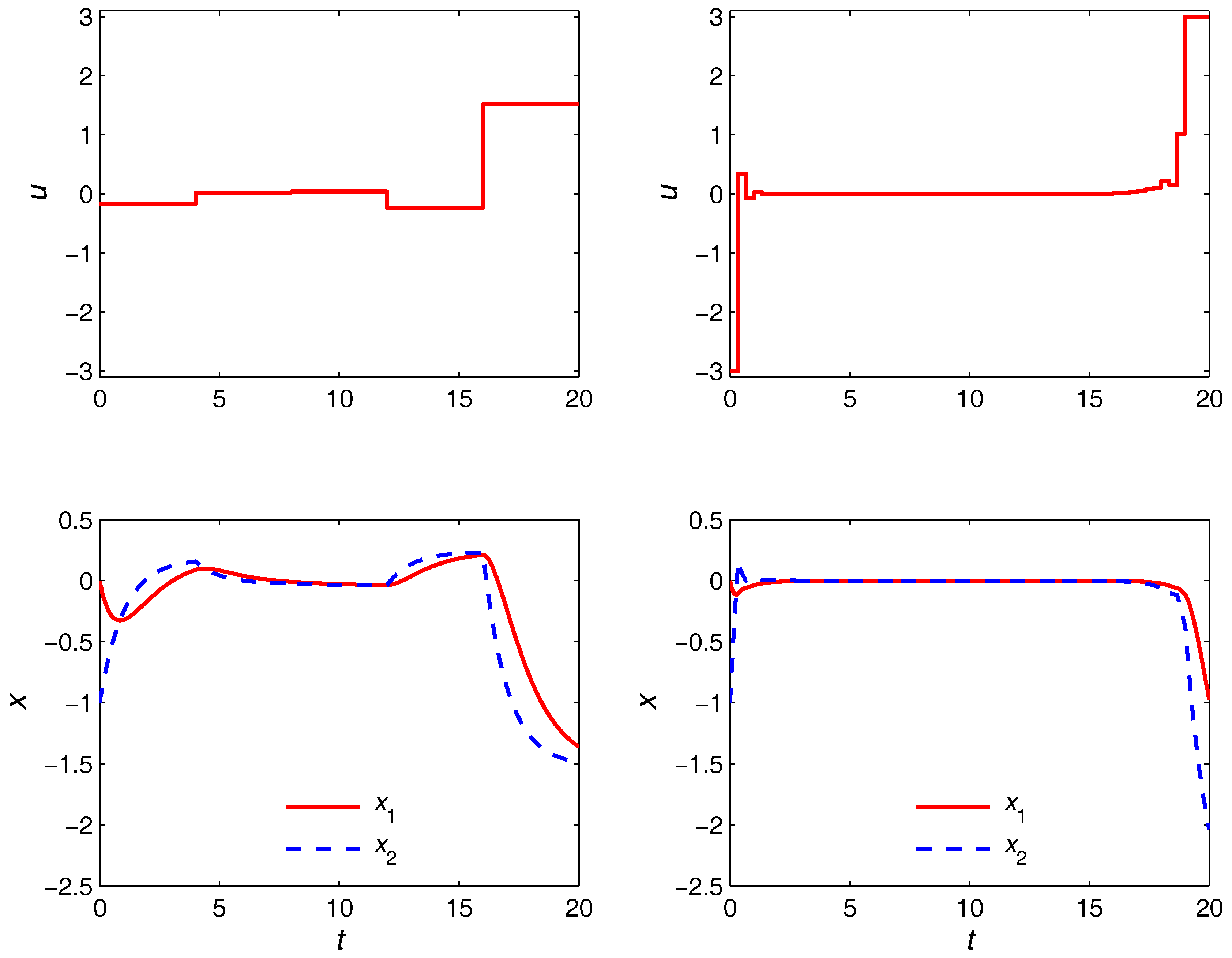
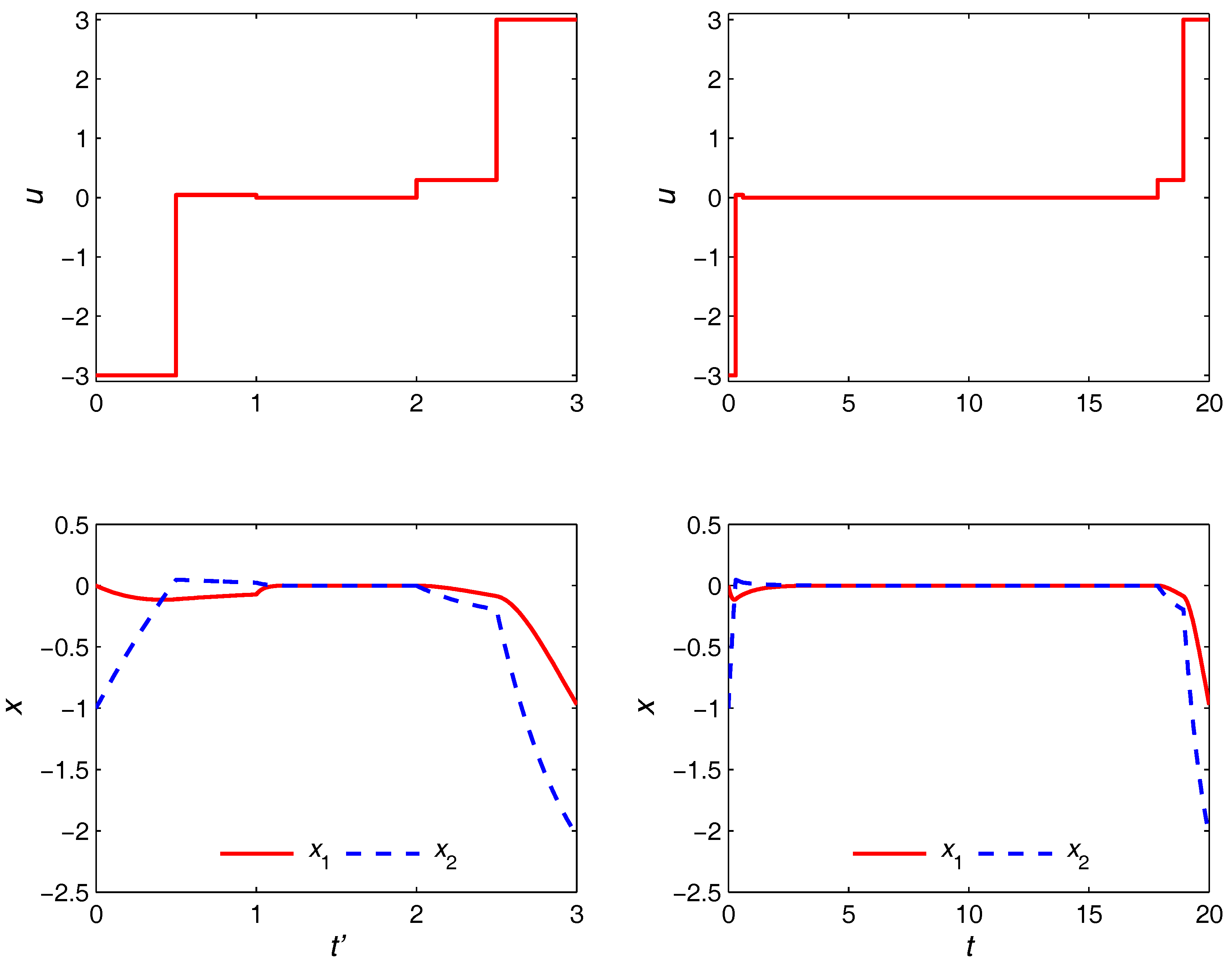
The optimal trajectories obtained from the nonuniform discretization strategy are given in Figure 5. It is seen that the steady-state turnpike is realized for both and cases. However, with the coarser discretization, the turnpike is realized only partially due to the limited number of control moves available and inability to adjust their switching times optimally. Specifically, the control u must depart from its optimal steady state as early as in order to use the remaining two epochs to satisfy the terminal equality constraint. On the other hand, with epochs, the turnpike is realized to (possibly) its full extent due to the much higher degree of freedom in the control moves. This is to be compared with the optimal trajectories in the right plot of Figure 6, where the proposed approach is shown to be able to yield quite the same trajectories with only five control moves. The durations of the transient and turnpike phases in this case are obtained as . The left plot in Figure 6 shows the optimal trajectories in the domain, in which the optimization problem is solved. Observe that the duration of each phase is 1 regardless of the values.
4.2. Example 2
This example considers a non-isothermal Van de Vusse reactor adapted from [46], in which the following reactions occur:
with B the desired product. The dynamic model of the reactor is given as:
where denotes the concentration of i; T and are the temperatures of the reactor and cooling jacket, respectively; V is the reaction volume; and is the outlet flowrate. Here, the original model in [46] has been modified to allow a varying volume. It is worth noting that, for the original model, conditions ensuring strict dissipativity, and, thus, potential emergence of turnpike have been verified in [27]. Nonetheless, such a result is not required in this work since it makes no assumption on the presence of a turnpike. The initial conditions are given as:
In addition, the model constants are provided in Table 2. For simplicity, the normalized heat transfer coefficients and are assumed to be independent of the volume V [47]. The operation takes h. As a safety precaution, the reactor temperature T must not exceed 110 °C anytime during the operation. Similarly, the concentration of D must not exceed 500 . At the final time, the reactor volume V must be 0.01 m3 or less. The optimization variables are the inlet flowrate and the cooling power , which are allowed to vary within m3 h−1 and kJ h−1, respectively. With the goal of maximizing the production of B, the dynamic optimization problem can be formulated as:
The optimal steady-state values required for the nonuniform discretization and proposed approaches are obtained from
where is the vector containing all the concentrations, and the steady-state model refers to the dynamic model (38) with the time derivatives set to zero. Notice that the path constraints on and T are included in Problem (41) as upper bounds for the corresponding variables. Except these and the lower bound of zero on the concentrations, other bounds on the state variables have no process implications and are placed so that the global solver can proceed. Once a global optimum is found, the solution must be checked to make sure these arbitrary bounds are not active.
The global solution of Problem (41) is obtained in less than s, with the optimum point m3 h−1, kJ h−1, mol m−3, °C, and m3.
The optimal solution and solver statistics for the different discretization strategies are given in Table 3. For the variant formulation of the proposed approach, the settings and are used. Similar to the previous example, the proposed approach yields a better optimal solution than the uniform discretization with the same number of epochs. The optimal solution of the latter improves by increasing the number of epochs to . Nonetheless, it is still inferior to the one obtained from the proposed approach with . Increasing N to 70 did not lead to an improved result as the solver failed after 207 iterations. The same problem occurred with . This shows that a finer discretization is not always beneficial in practice as it can lead to numerical issues. Similarly, the nonuniform discretization with terminated with a failure message indicating local infeasibility. However, this problem is known to be feasible because a more constrained version of it, i.e., the proposed semi-uniform discretization approach with , is feasible (see Table 3). Therefore, the reported local infeasibility is only due to numerical issues that apparently arise from including the duration of epochs as extra optimization variables. In terms of the solution speed, the CPU times show that the proposed approach (main formulation) converges to a better solution about 10 times faster than the uniform discretization with . This is in spite of the significantly more iterations that are taken by the proposed approach. The speed-up is even more remarkable for the variant formulation, i.e., about 37-fold.
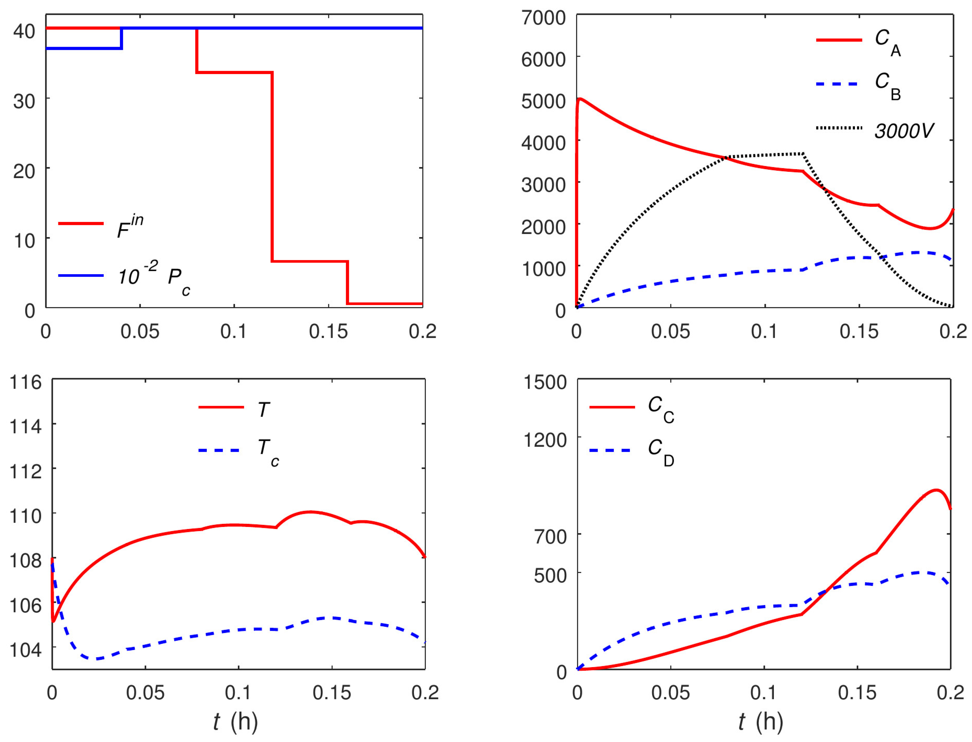
The optimal trajectories for control variables and a selection of the state variables in the case of the uniform discretization with and the proposed approach (both variants) are plotted in Figure 7 and Figure 8, respectively. The units for the quantities are consistent with those reported in Table 2. Similar observations as in the previous example hold here, and are omitted for brevity. The only notable additional point is that, here, the optimal trajectories from the main and the variant formulations are not exactly the same, although the difference can hardly be noticed. Moreover, the main and the variant formulations converge to slightly different values for the triplet , i.e., and h for the main and variant formulations, respectively. The optimal objective value from both formulations, however, is almost the same despite the slight difference in the computed optima.
Shorter Time Horizon
Here, the Van de Vusse reactor is revisited with a time horizon that is too short for the turnpike to appear. The purpose of this case study is to show that the proposed discretization approach still works in such conditions, although it may not be computationally more efficient than conventional discretization. To this end, the final time is reduced to h, and the problem is solved using the uniform discretization with and the proposed approach with (). The computational results are given in Table 4, and the optimal trajectories for the case of are plotted in Figure 9 and Figure 10. It is seen that the optimal trajectories do not reach a steady-state turnpike. Despite this, the proposed approach is still able to solve the problem, and even converge to a slightly better solution than the uniform discretization with . The durations of the transient and turnpike phases are obtained as h. Interestingly enough, it is seen that the duration of the turnpike is pushed to zero by the optimizer, reducing the effective number of epochs to four. The convergence to a better solution despite the absence of a turnpike and lower number of epochs can be explained by the inherent flexibility of the proposed approach in adjusting the location and duration of epochs. Note, however, that the uniform discretization with is able to yield yet an improved solution. In both cases, the solution with the uniform discretization converges somewhat faster, than the proposed approach. This suggests that, for very short time horizons, the extra computational overhead introduced by the proposed approach may not be offset by the reduction in the number of epochs.
4.3. Example 3
Finally, dynamic optimization of a continuous stirred-tank reactor adapted from [47] is presented. The following reactions take place in the reactor:
where P and I are the desired and undesired products, respectively; and are the kinetic constants. Two pure streams at the flowrates and and concentrations and , respectively, enter the reactor. The reactor is modeled as:
with being the outlet flow rate, where is a positive constant, and the initial conditions are given by
The model parameters and the initial conditions are found in Table 5. The operation takes min, and the objective is to maximize production of P during this period. The inlet flow rates are taken as the optimization variables. The following dynamic optimization problem is formulated:
The optimal steady-state values required for the nonuniform discretization and proposed approaches are obtained from
where is the vector containing all the concentrations, and the steady-state model refers to Problem (42) with the time derivatives set to zero. Similar to the previous example, bounds on the volume and the concentrations of A, B, and P have no process implications and are placed so that the global solver can proceed. The obtained global solution is accepted if these arbitrary bounds are not active.
The global solution of Problem (45) is obtained in 0.016 s, with the optimum point L min−1, mol L−1, and L.
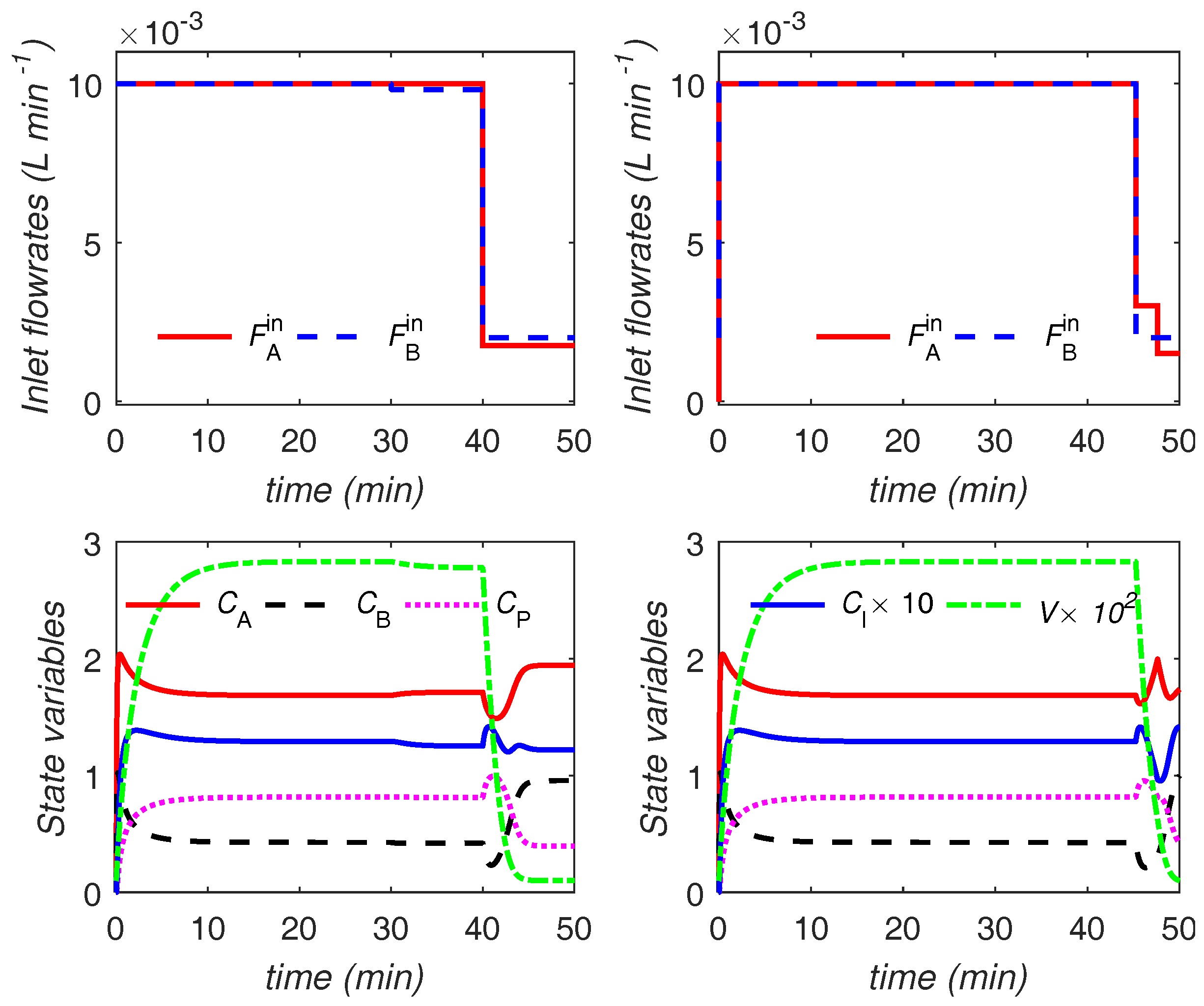
Table 6 shows the optimal solution and solver statistics for the uniform, nonuniform, and proposed discretization strategies. The tolerances and are used for the variant formulation of the proposed approach. With epochs, the proposed strategy and its variant yield a considerably improved solution compared to the uniform discretization. The variant formulation outperforms the main one in both number of iterations and CPU time. It also slightly outperforms the uniform discretization with in the same respects. The durations of the transient and turnpike phases for the proposed approach (both formulations) are obtained as min.
The uniform strategy converges to the same solution with a much higher number of epochs () and a markedly higher computational time (93% and 200% slower compared to the main and variant formulations, respectively). Here, the nonuniform strategy converges quite closely to the optimal solution of with only two epochs. With only one more epoch, the nonuniform strategy is able to reach this solution (and slightly improves upon it). Nonetheless, the solution takes a much higher CPU time than the one with the proposed strategy, i.e, 1.8 and 2.8 times higher than the main and variant formulations, respectively. The durations of the three epochs used by the nonuniform discretization are obtained as min.
5. Conclusions
A new adaptive control discretization approach for efficient dynamic optimization is proposed. The approach is based on turnpike theory in optimal control and is most suitable for continuous systems with sufficiently long time horizons during which steady state is likely to emerge. However, it can also be applied to other systems with a steady-state solution, whether or not the steady state will actually appear in the solution trajectories. The special semi-uniform discretization enables approximating the turnpike structure with a minimal number of epochs, while avoiding the robustness issues that can be encountered with a full nonuniform discretization strategy. Unlike some other adaptive discretization techniques, the proposed adaptive discretization is built directly into the problem formulation. Thus, one would need to solve only one optimization problem instead of a series of successively refined problems. Another advantage of the proposed approach is the use of globally optimal steady-state values in the formulation that helps the optimizer avoid suboptimal solutions in case a steady-state turnpike emerges. It is shown that the proposed approach, especially the variant formulation, can significantly reduce the computational cost of dynamic optimization for systems of interest. However, a downside of the variant formulation is that the tolerance values can impact the performance of the numerical solution, and finding appropriate values for them may not be trivial. In this case, one may choose to use the main formulation instead, as it is adequately superior and requires no tuning parameters. Future work may include applying the proposed approach to large-scale processes and optimal campaign continuous manufacturing problems, as described in [47].
Acknowledgments
Financial support from the Novartis-MIT Center for Continuous Manufacturing (Cambridge, MA, USA) is gratefully acknowledged.
Author Contributions
This work was done under the supervision of Paul I. Barton. Both authors contributed to the development of the proposed approach. Ali M. Sahlodin also performed the case studies and prepared the manuscript.
Conflicts of Interest
The authors declare no conflict of interest.
References
- Cervantes, A.; Biegler, L. Optimization Strategies for Dynamic Systems. In Encyclopedia of Optimization; Floudas, C.A., Pardalos, P.M., Eds.; Springer: Boston, MA, USA, 2009; pp. 2847–2858. [Google Scholar]
- Chachuat, B. Nonlinear and Dynamic Optimization: From Theory to Practice-IC-32: Spring Term 2009; Polycopiés de l’EPFL, EPFL: Lausanne, Switzerland, 2009. [Google Scholar]
- Von Stryk, O.; Bulirsch, R. Direct and indirect methods for trajectory optimization. Ann. Oper. Res. 1992, 37, 357–373. [Google Scholar] [CrossRef]
- Biegler, L. An overview of simultaneous strategies for dynamic optimization. Chem. Eng. Process. 2007, 46, 1043–1053. [Google Scholar] [CrossRef]
- Kraft, D. On Converting Optimal Control Problems into Nonlinear Programming Problems. In Computational Mathematical Programming; Schittkowski, K., Ed.; Springer: Berlin/Heidelberg, Germany, 1985; Volume 15, pp. 261–280. [Google Scholar]
- Binder, T.; Blank, L.; Bock, H.; Bulirsch, R.; Dahmen, W.; Diehl, M.; Kronseder, T.; Marquardt, W.; Schlöder, J.; von Stryk, O. Introduction to Model Based Optimization of Chemical Processes on Moving Horizons. In Online Optimization of Large Scale Systems; Grötschel, M., Krumke, S., Rambau, J., Eds.; Springer: Berlin/Heidelberg, Germany, 2001; pp. 295–339. [Google Scholar]
- Hartwich, A.; Marquardt, W. Dynamic optimization of the load change of a large-scale chemical plant by adaptive single shooting. Comput. Chem. Eng. 2010, 34, 1873–1889. [Google Scholar] [CrossRef]
- Binder, T.; Blank, L.; Dahmen, W.; Marquardt, W. Grid refinement in multiscale dynamic optimization. In European Symposium on Computer Aided Process Engineering-10; Pierucci, S., Ed.; Elsevier: Amsterdam, The Netherlands, 2000; Volume 8, pp. 31–36. [Google Scholar]
- Feehery, W.F.; Tolsma, J.E.; Barton, P.I. Efficient sensitivity analysis of large-scale differential-algebraic systems. Appl. Numer. Math. 1997, 25, 41–54. [Google Scholar] [CrossRef]
- Özyurt, D.B.; Barton, P.I. Cheap Second Order Directional Derivatives of Stiff ODE Embedded Functionals. SIAM J. Sci. Comput. 2005, 26, 1725–1743. [Google Scholar] [CrossRef]
- Özyurt, D.B.; Barton, P.I. Large-Scale Dynamic Optimization Using the Directional Second-Order Adjoint Method. Ind. Eng. Chem. Res. 2005, 44, 1804–1811. [Google Scholar] [CrossRef]
- Luus, R.; Cormack, D.E. Multiplicity of solutions resulting from the use of variational methods in optimal control problems. Can. J. Chem. Eng. 1972, 50, 309–311. [Google Scholar] [CrossRef]
- Luus, R.; Dittrich, J.; Keil, F.J. Multiplicity of solutions in the optimization of a bifunctional catalyst blend in a tubular reactor. Can. J. Chem. Eng. 1992, 70, 780–785. [Google Scholar] [CrossRef]
- Banga, J.R.; Seider, W.D. Global optimization of chemical processes using stochastic algorithms. In State of the Art in Global Optimization: Computational Methods and Applications; Floudas, C., Pardalos, P., Eds.; Kluwer Academic Publishers: Dordrecht, The Netherlands, 1996; pp. 563–583. [Google Scholar]
- Srinivasan, B.; Primus, C.; Bonvin, D.; Ricker, N. Run-to-run optimization via control of generalized constraints. Control Eng. Pract. 2001, 9, 911–919. [Google Scholar] [CrossRef]
- Binder, T.; Cruse, A.; Villar, C.C.; Marquardt, W. Dynamic optimization using a wavelet based adaptive control vector parameterization strategy. Comput. Chem. Eng. 2000, 24, 1201–1207. [Google Scholar] [CrossRef]
- Schlegel, M.; Stockmann, K.; Binder, T.; Marquardt, W. Dynamic optimization using adaptive control vector parameterization. Comput. Chem. Eng. 2005, 29, 1731–1751. [Google Scholar] [CrossRef]
- Schlegel, M.; Marquardt, W. Detection and exploitation of the control switching structure in the solution of dynamic optimization problems. J. Process Control 2006, 16, 275–290. [Google Scholar] [CrossRef]
- Schlegel, M. Adaptive Discretization Methods for the Efficient Solution of Dynamic Optimization Problems; VDI-Verlag: Dusseldorf, Germany, 2005. [Google Scholar]
- Liu, P.; Li, G.; Liu, X.; Zhang, Z. Novel non-uniform adaptive grid refinement control parameterization approach for biochemical processes optimization. Biochem. Eng. J. 2016, 111, 63–74. [Google Scholar] [CrossRef]
- Dorfman, R.; Samuelson, P.A.; Solow, R.M. Linear Programming and Economic Analysis; McGraw Hill: New York, NY, USA, 1958. [Google Scholar]
- McKenzie, L. Turnpike theory. Econometrica 1976, 44, 841–865. [Google Scholar] [CrossRef]
- Wilde, R.; Kokotovic, P. A dichotomy in linear control theory. IEEE Trans. Autom. Control 1972, 17, 382–383. [Google Scholar] [CrossRef]
- Anderson, B.D.; Kokotovic, P.V. Optimal control problems over large time intervals. Automatica 1987, 23, 355–363. [Google Scholar] [CrossRef]
- Rao, A.; Mease, K. Dichotomic basis approach to solving hyper-sensitive optimal control problems. Automatica 1999, 35, 633–642. [Google Scholar] [CrossRef]
- Grüne, L.; Müller, M.A. On the relation between strict dissipativity and turnpike properties. Syst. Control Lett. 2016, 90, 45–53. [Google Scholar] [CrossRef]
- Faulwasser, T.; Korda, M.; Jones, C.N.; Bonvin, D. On turnpike and dissipativity properties of continuous-time optimal control problems. Automatica 2017, 81, 297–304. [Google Scholar] [CrossRef]
- Galán, S.; Feehery, W.F.; Barton, P.I. Parametric sensitivity functions for hybrid discrete/continuous systems. Appl. Numer. Math. 1999, 31, 17–47. [Google Scholar] [CrossRef]
- Rawlings, J.; Amrit, R. Optimizing Process Economic Performance Using Model Predictive Control. In Nonlinear Model Predictive Control; Magni, L., Raimondo, D., Allgöwer, F., Eds.; Springer: Berlin/Heidelberg, Germany, 2009; Volume 384, pp. 119–138. [Google Scholar]
- Carlson, D.; Haurie, A.; Leizarowitz, A. Infinite Horizon Optimal Control: Deterministic and Stochastic Systems; Springer: Berlin/Heidelberg, Germany, 1991. [Google Scholar]
- Zaslavski, A.J. Turnpike Properties in the Calculus of Variations and Optimal Control; Springer: New York, NY, USA, 2006. [Google Scholar]
- Zaslavski, A.J. Turnpike Properties of Optimal Control Systems. Aenorm 2012, 20, 36–40. [Google Scholar]
- Zaslavski, A.J. Turnpike Phenomenon and Infinite Horizon Optimal Control; Springer: Cham, Switzerland, 2014. [Google Scholar]
- Faulwasser, T.; Korda, M.; Jones, C.N.; Bonvin, D. Turnpike and dissipativity properties in dynamic real-time optimization and economic MPC. In Proceedings of the 2014 IEEE 53rd Annual Conference on Decision and Control (CDC), Los Angeles, CA, USA, 15–17 December 2014; pp. 2734–2739. [Google Scholar]
- Grüne, L. Economic receding horizon control without terminal constraints. Automatica 2013, 49, 725–734. [Google Scholar] [CrossRef]
- Faulwasser, T.; Bonvin, D. On the design of economic NMPC based on approximate turnpike properties. In Proceedings of the 2015 54th IEEE Conference on Decision and Control (CDC), Osaka, Japan, 15–18 December 2015; pp. 4964–4970. [Google Scholar]
- Trélat, E.; Zuazua, E. The turnpike property in finite-dimensional nonlinear optimal control. J. Differ. Equ. 2015, 258, 81–114. [Google Scholar] [CrossRef]
- Teo, K.L.; Jennings, L.S.; Lee, H.W.J.; Rehbock, V. The control parameterization enhancing transform for constrained optimal control problems. ANZIAM J. 1999, 40, 314–335. [Google Scholar] [CrossRef]
- Lee, H.; Teo, K.; Rehbock, V.; Jennings, L. Control parametrization enhancing technique for optimal discrete-valued control problems. Automatica 1999, 35, 1401–1407. [Google Scholar] [CrossRef]
- Li, R.; Teo, K.; Wong, K.; Duan, G. Control parameterization enhancing transform for optimal control of switched systems. Math. Comput. Model. 2006, 43, 1393–1403. [Google Scholar] [CrossRef]
- Wächter, A.; Biegler, L.T. On the implementation of an interior-point filter line-search algorithm for large-scale nonlinear programming. Math. Program. 2006, 106, 25–57. [Google Scholar] [CrossRef]
- Tolsma, J.; Barton, P.I. DAEPACK: An Open Modeling Environment for Legacy Models. Ind. Eng. Chem. Res. 2000, 39, 1826–1839. [Google Scholar] [CrossRef]
- Tolsma, J.E.; Barton, P.I. Hidden Discontinuities and Parametric Sensitivity Calculations. SIAM J. Sci. Comput. 2002, 23, 1861–1874. [Google Scholar] [CrossRef]
- Tawarmalani, M.; Sahinidis, N.V. A polyhedral branch-and-cut approach to global optimization. Math. Program. 2005, 103, 225–249. [Google Scholar] [CrossRef]
- GAMS. GAMS–A User’s Guide. Available online: https://www.gams.com/24.8/docs/userguides/GAMSUsersGuide.pdf (accessed on 14 December 2017).
- Rothfuss, R.; Rudolph, J.; Zeitz, M. Flatness based control of a nonlinear chemical reactor model. Automatica 1996, 32, 1433–1439. [Google Scholar] [CrossRef]
- Sahlodin, A.M.; Barton, P.I. Optimal Campaign Continuous Manufacturing. Ind. Eng. Chem. Res. 2015, 54, 11344–11359. [Google Scholar] [CrossRef]
Figure 1.
An optimal control or state trajectory with two transient phases and a turnpike in between. The green solid line represents the (globally) optimal steady state or , and the red dashed lines denote its -neighborhood.
Figure 1.
An optimal control or state trajectory with two transient phases and a turnpike in between. The green solid line represents the (globally) optimal steady state or , and the red dashed lines denote its -neighborhood.

Figure 2.
Schematic of an optimal control trajectory resulting from a nonuniform discretization. The dashed line illustrates the ideal optimal trajectory that might be obtained without discretization.
Figure 2.
Schematic of an optimal control trajectory resulting from a nonuniform discretization. The dashed line illustrates the ideal optimal trajectory that might be obtained without discretization.

Figure 3.
Schematic of the semi-uniform control discretization in the real time domain t (left) and the transformed time domain (right). The three transient and turnpike phases are delineated by the blue dashed lines.
Figure 3.
Schematic of the semi-uniform control discretization in the real time domain t (left) and the transformed time domain (right). The three transient and turnpike phases are delineated by the blue dashed lines.
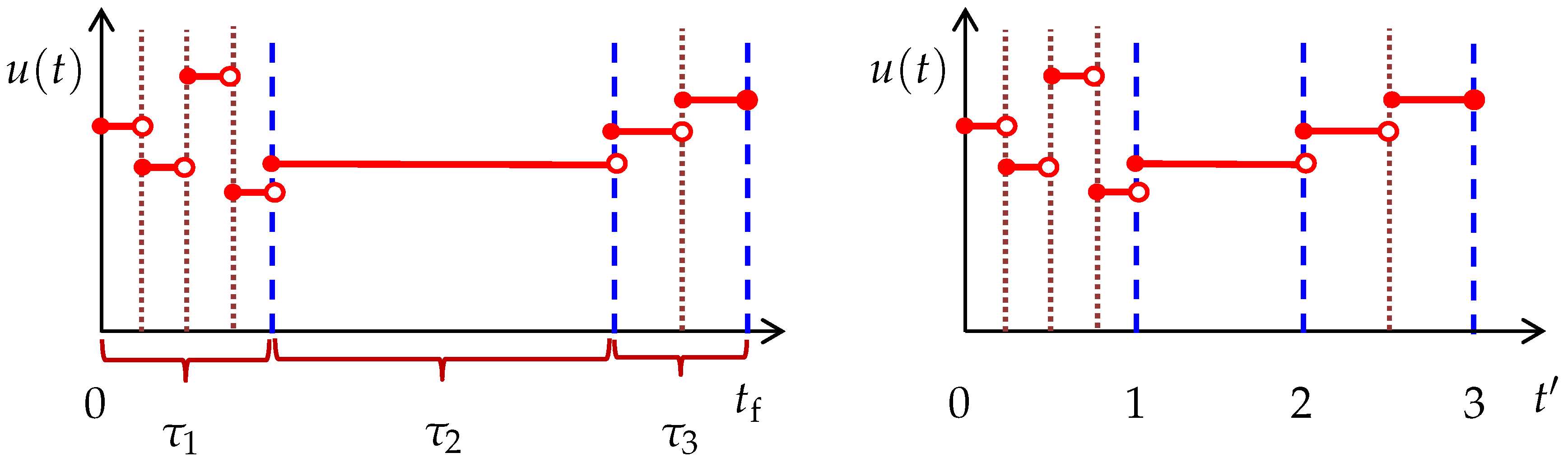
Figure 4.
Adaptive semi-uniform discretization with suboptimal (left) and optimal (right) solution for s. The dashed line trajectory shows the ideal optimal control as a reference.
Figure 4.
Adaptive semi-uniform discretization with suboptimal (left) and optimal (right) solution for s. The dashed line trajectory shows the ideal optimal control as a reference.
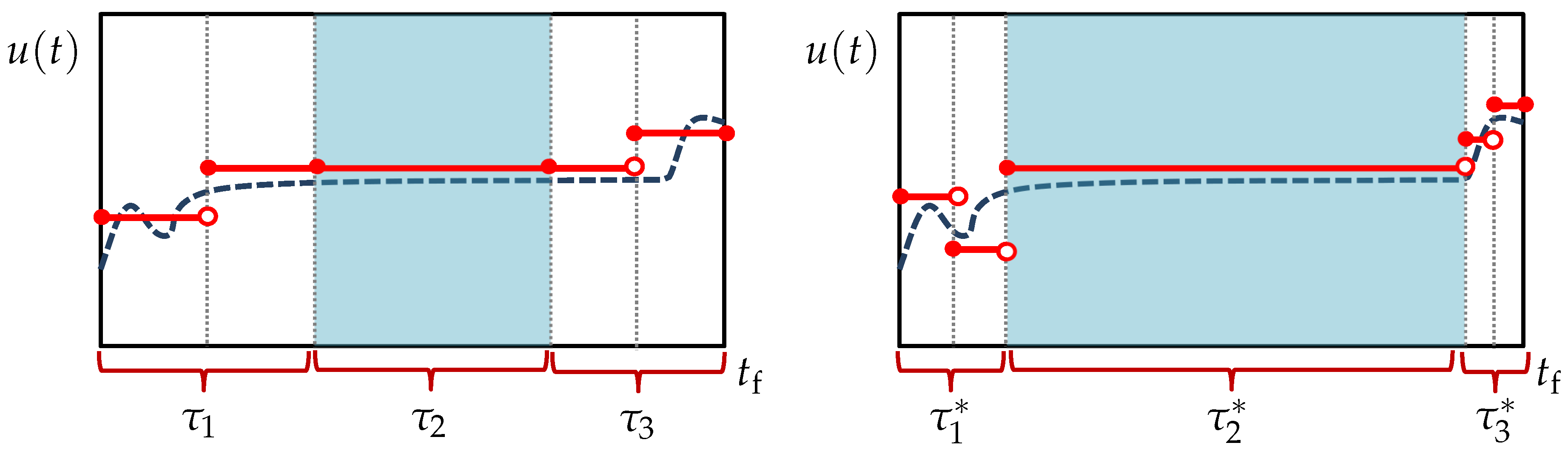
Figure 5.
Optimal trajectories for Problem (37) in case of a uniform discretization with (left) and (right) epochs.
Figure 5.
Optimal trajectories for Problem (37) in case of a uniform discretization with (left) and (right) epochs.

Figure 6.
Optimal trajectories for Problem (37) in case of the proposed semi-uniform discretization approach with epochs (both the main and variant formulations) in the (left) and t (right) domains.
Figure 6.
Optimal trajectories for Problem (37) in case of the proposed semi-uniform discretization approach with epochs (both the main and variant formulations) in the (left) and t (right) domains.

Figure 7.
Optimal trajectories for Problem (40) in the case of a uniform discretization with (left) and (right) epochs.
Figure 7.
Optimal trajectories for Problem (40) in the case of a uniform discretization with (left) and (right) epochs.
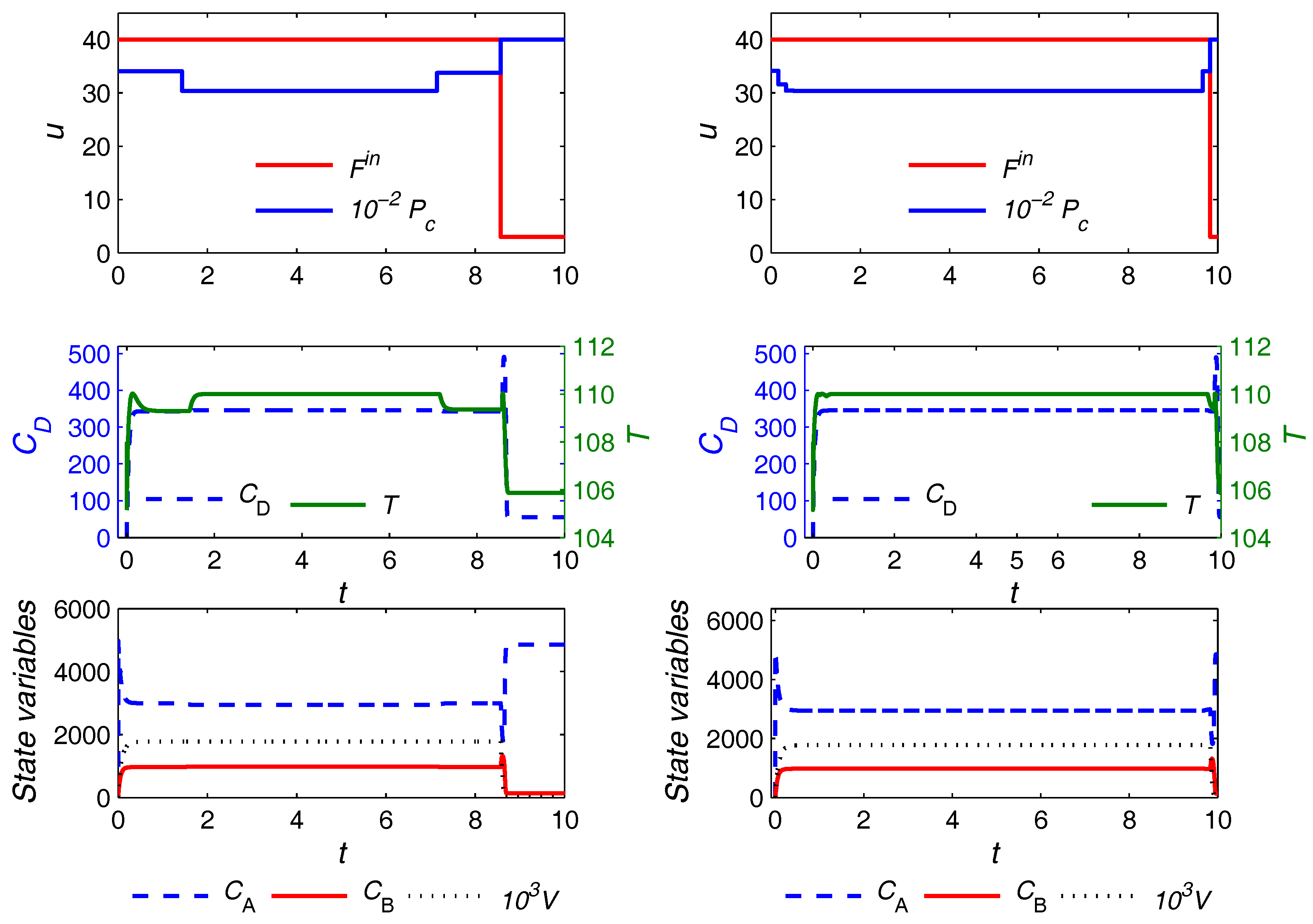
Figure 8.
Optimal trajectories for Problem (40) in the case of the main (left) and the variant (right) formulations of the proposed approach with epochs.
Figure 8.
Optimal trajectories for Problem (40) in the case of the main (left) and the variant (right) formulations of the proposed approach with epochs.
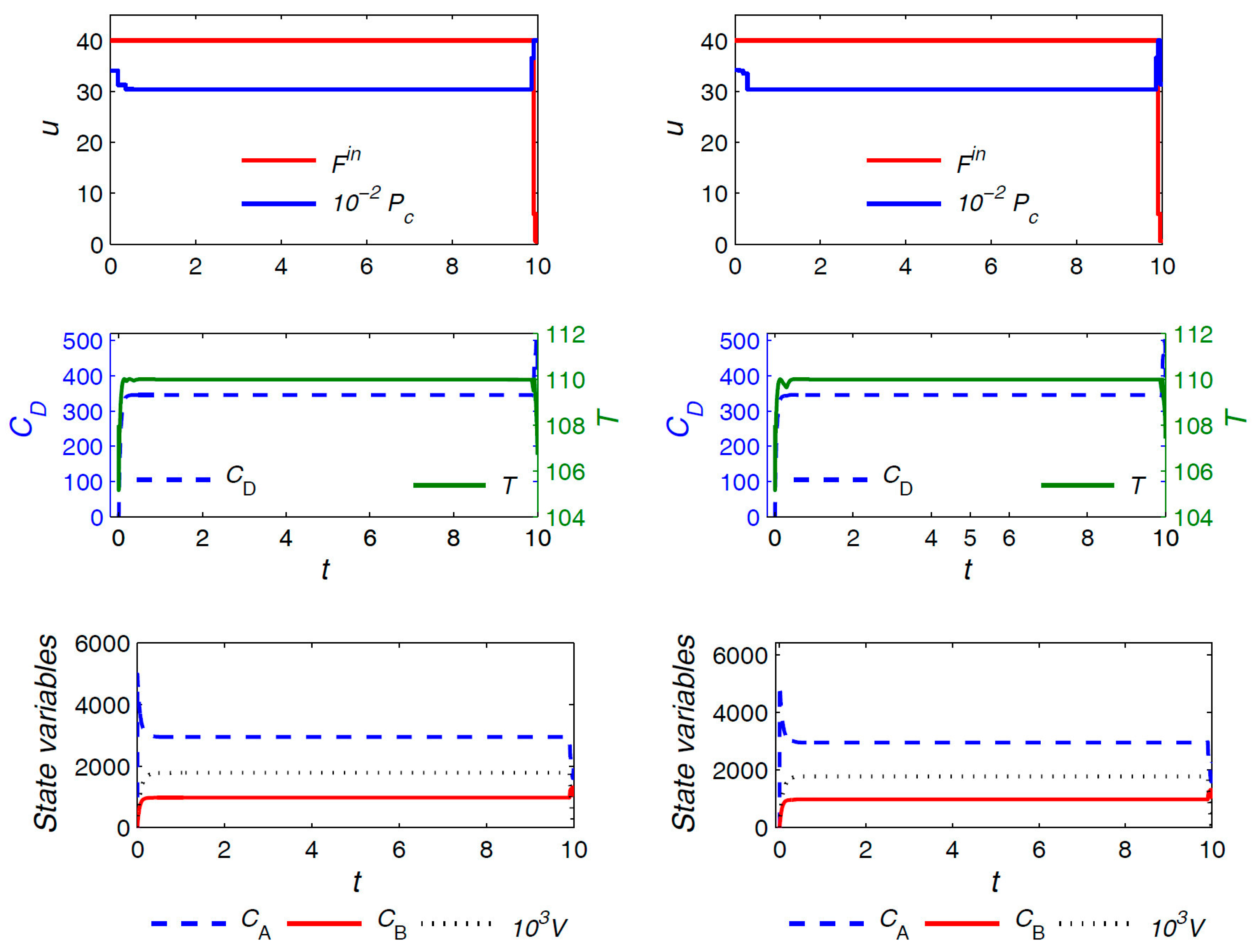
Figure 9.
Optimal trajectories for Problem (40) with a short time horizon solved using a uniform discretization and epochs.
Figure 9.
Optimal trajectories for Problem (40) with a short time horizon solved using a uniform discretization and epochs.

Figure 10.
Optimal trajectories for Problem (40) with a short time horizon solved using the proposed approach and epochs.
Figure 10.
Optimal trajectories for Problem (40) with a short time horizon solved using the proposed approach and epochs.

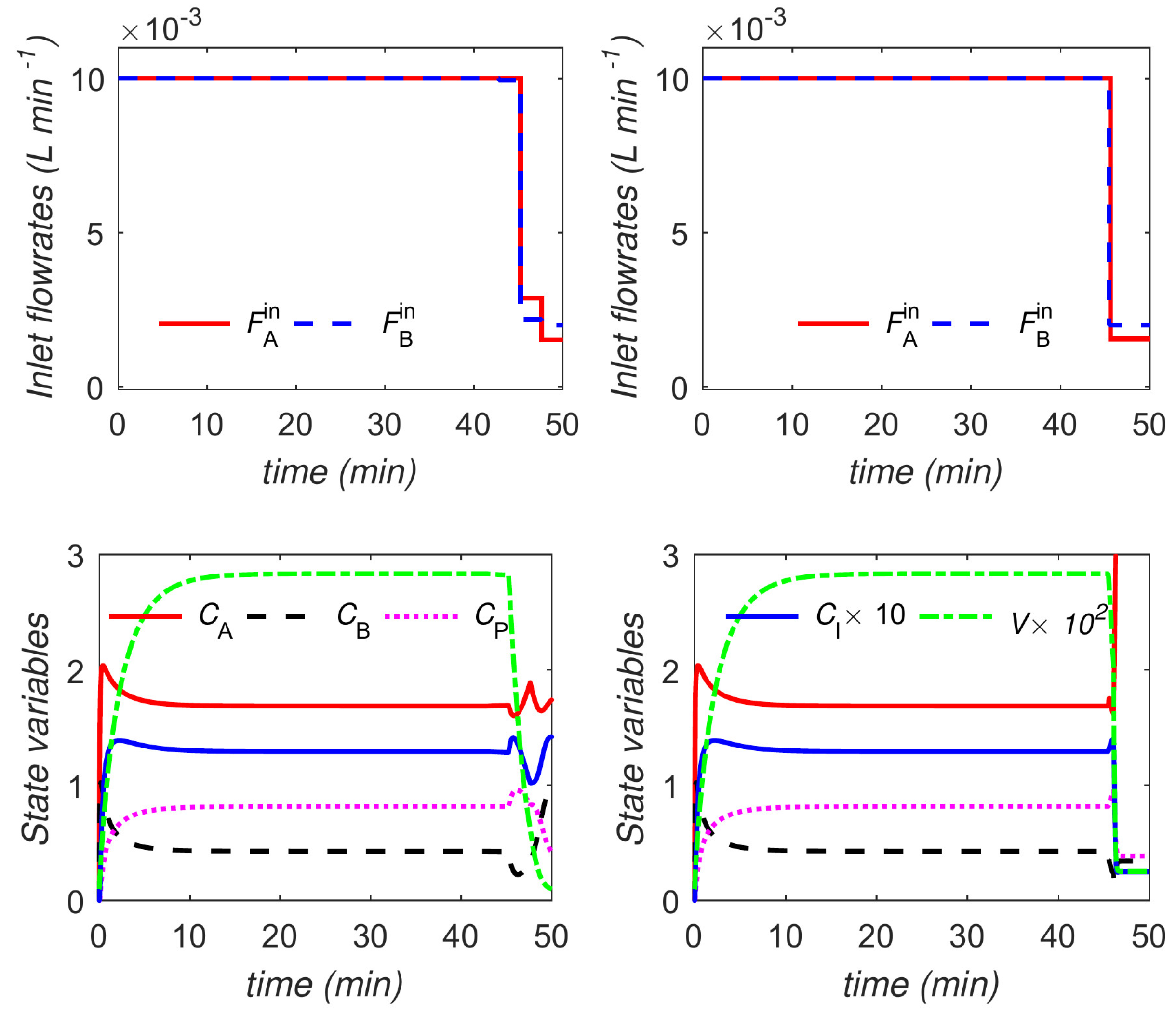
Figure 11.
Optimal trajectories for Problem (44) in the case of the uniform (left) and proposed (right) discretization methods both with epochs.
Figure 11.
Optimal trajectories for Problem (44) in the case of the uniform (left) and proposed (right) discretization methods both with epochs.

Figure 12.
Optimal trajectories for Problem (44) in the case of the uniform discretization with (left) and the nonuniform discretization with (right) epochs.
Figure 12.
Optimal trajectories for Problem (44) in the case of the uniform discretization with (left) and the nonuniform discretization with (right) epochs.

Table 1.
Optimal objective values, number of iterations, and CPU times for different discretization strategies in Problem (37). denotes the total number of optimization variables for each strategy.
Table 1.
Optimal objective values, number of iterations, and CPU times for different discretization strategies in Problem (37). denotes the total number of optimization variables for each strategy.
| Discretization | N | Iter | CPU (s) | ||
|---|---|---|---|---|---|
| Uniform | 5 | 5 | 9.32 | 13 | 0.13 |
| Uniform | 60 | 60 | 2.45 | 103 | 8.02 |
| Nonuniform | 5 | 9 | not converged | >1000 | >11 |
| Proposed | 5 () | 7 | 2.45 | 38 | 0.79 |
| Proposed (variant) | 5 () | 7 | 2.45 | 33 | 0.89 |
Table 2.
Constants for the Van de Vusse reactor model (38).
Table 2.
Constants for the Van de Vusse reactor model (38).
| 1.29 | h−1 | 30.828 | h−1 | ||
| 9.04 | m3 (mol h)−1 | 86.688 | h−1 | ||
| 9758.3 | K | 0.1 | K kJ−1 | ||
| 8560 | K | 3.52 | m3 K kJ−1 | ||
| 4.2 | kJ mol−1 | 30 | m3/2 h−1 | ||
| −11 | kJ mol−1 | 104.9 | °C | ||
| −41.85 | kJ mol−1 | 5.10 | mol m−3 |
Table 3.
Optimal objective values, number of iterations, and CPU times for different discretization strategies in Problem (40). denotes the total number of optimization variables for each strategy.
Table 3.
Optimal objective values, number of iterations, and CPU times for different discretization strategies in Problem (40). denotes the total number of optimization variables for each strategy.
| Discretization | N | Iter | CPU (s) | ||
|---|---|---|---|---|---|
| Uniform | 7 | 14 | −3.34 | 251 | 14.7 |
| Uniform | 60 | 120 | −3.84 | 227 | 798 |
| Uniform | 70 | 140 | failed | 207 | 645 |
| Uniform | 80 | 160 | failed | 295 | 1160 |
| Nonuniform | 7 | 19 | failed | 1212 | 134 |
| Proposed | 7 () | 15 | −3.87 | 800 | 75.2 |
| Proposed (variant) | 7 () | 15 | −3.87 | 210 | 21.4 |
Table 4.
Optimal objective values, number of iterations, and CPU times for different discretization strategies in Problem (40) for the case of a short time horizon.
Table 4.
Optimal objective values, number of iterations, and CPU times for different discretization strategies in Problem (40) for the case of a short time horizon.
| Discretization | N | Iter | CPU (s) | ||
|---|---|---|---|---|---|
| Uniform | 5 | 10 | 3987 | 44 | 1.65 |
| Uniform | 7 | 14 | 4058 | 53 | 2.29 |
| Proposed | 5 () | 11 | 4009 | 69 | 2.77 |
| Proposed (variant) | 5 () | 11 | 4009 | 53 | 2.33 |
Table 5.
Constants and initial conditions for the model (42).
Table 5.
Constants and initial conditions for the model (42).
| Parameters | Initial Conditions | ||||
|---|---|---|---|---|---|
| 0.8 | L (mol min)−1 | 0 | mol L−1 | ||
| 0.5 | L (mol min)−1 | 0 | mol L−1 | ||
| 5 | mol L−1 | 0 | mol L−1 | ||
| 3 | mol L−1 | 0 | mol L−1 | ||
| 0.119 | L1/2 min−1 | 0.001 | L | ||
Table 6.
Optimal objective values, number of iterations, and CPU times for different discretization strategies in Problem (44). denotes the total number of optimization variables for each strategy.
Table 6.
Optimal objective values, number of iterations, and CPU times for different discretization strategies in Problem (44). denotes the total number of optimization variables for each strategy.
| Discretization | N | Iter | CPU (s) | ||
|---|---|---|---|---|---|
| Uniform | 5 | 10 | 0.66 | 31 | 1.3 |
| Uniform | 14 | 28 | 0.734 | 23 | 1.26 |
| Uniform | 20 | 40 | 0.739 | 27 | 2.38 |
| Uniform | 21 | 42 | 0.741 | 34 | 3.53 |
| Nonuniform | 2 | 4 | 0.731 | 35 | 0.59 |
| Nonuniform | 3 | 7 | 0.742 | 145 | 3.28 |
| Proposed | 5 () | 11 | 0.741 | 29 | 1.83 |
| Proposed (variant) | 5 () | 11 | 0.741 | 24 | 1.18 |
© 2017 by the authors. Licensee MDPI, Basel, Switzerland. This article is an open access article distributed under the terms and conditions of the Creative Commons Attribution (CC BY) license (http://creativecommons.org/licenses/by/4.0/).
Share and Cite
MDPI and ACS Style
Sahlodin, A.M.; Barton, P.I. Efficient Control Discretization Based on Turnpike Theory for Dynamic Optimization. Processes 2017, 5, 85. https://doi.org/10.3390/pr5040085
AMA Style
Sahlodin AM, Barton PI. Efficient Control Discretization Based on Turnpike Theory for Dynamic Optimization. Processes. 2017; 5(4):85. https://doi.org/10.3390/pr5040085
Chicago/Turabian StyleSahlodin, Ali M., and Paul I. Barton. 2017. "Efficient Control Discretization Based on Turnpike Theory for Dynamic Optimization" Processes 5, no. 4: 85. https://doi.org/10.3390/pr5040085
Note that from the first issue of 2016, this journal uses article numbers instead of page numbers. See further details here.