Statistical Analysis of Circulating Water Quality Parameters under Variable-Frequency Vertical Electromagnetic Fields

1
School of Technology, Beijing Forestry University, Beijing 100083, China
2
School of Automation Engineering, Northeast Electric Power University, Jilin 132012, China
*
Author to whom correspondence should be addressed.
Processes 2018, 6(10), 182; https://doi.org/10.3390/pr6100182
Submission received: 7 September 2018
/
Revised: 29 September 2018
/
Accepted: 1 October 2018
/
Published: 2 October 2018
(This article belongs to the Special Issue Wastewater Treatment Processes)
Abstract
:No unified electromagnetic anti-fouling mechanism is currently available. Most research has focused on the effects of structural parameters and water quality parameters on electromagnetic fields; variations in water quality parameters under the influence of electromagnetic fields have not been reported. A variable-frequency vertical electromagnetic field is proposed in this study. Relationships between conductivity, pH value, dissolved oxygen, turbidity, fouling resistance, and magnetic acting time were carefully analyzed using statistical analysis. Results show that the conductivity difference was the most explanatory predictive variable on magnetic acting time in the multiple stepwise regression model. Magnetic acting time has a greater impact on conductivity than pH value and dissolved oxygen. Conductivity is used as an adaptive feedback control parameter for the optimum anti-fouling state. Fouling resistance on the heat-exchanging surface of the magnetic experiment was smaller than that of the contrast experiment. The anti-fouling efficiency in 1 kHz and 5 kHz magnetic and contrast experiments was 91.23% and 46.97%, respectively. Better anti-fouling performance was realized under the influence of low-frequency electromagnetic fields, confirming that physical water treatment is an effective and environmentally friendly method to eliminate heat exchanger fouling. This research serves as a reference for the development of an electromagnetic-adaptive closed-loop water treatment device.
1. Introduction
Variable-frequency electromagnetic water treatment technology is used due to its environmental nature and easy operation. However, the anti-fouling mechanism is imperfect, and most research has focused on the effects of structural and water quality parameters on the electromagnetic field. Suitable feedback parameters must be included in experiments [1,2,3]. Basic research on variations in physical, chemical, and biological water quality parameters under the influence of an electromagnetic field has been conducted [4,5]. Based on objective actual measurements, statistical analysis has tended to focus on the robustness of data and is particularly applicable to inner regularity in a quantitative form. Electromagnetic water treatment has rarely been studied using statistical analysis methods [6,7,8].
Variations in water quality parameters explain electromagnetic parameters to different extents. This study proposes an online fouling prevention and effect evaluation water treatment experiment [9,10]. Variations in conductivity, pH value, dissolved oxygen, turbidity, and fouling resistance under the influence of a variable-frequency electromagnetic field are carefully analyzed. Statistical analysis is used to verify the importance of water quality parameters in the fouling formation process. The degrees and effects of heat transfer, fouling abscission, and fouling inhibition are obtained, and a mathematical model of electromagnetic and water quality parameters is established [11].
2. Materials and Methods
2.1. Experimental System
The principle of online fouling prevention and effect evaluation water treatment experiment is shown in Figure 1. An experimental system with a double pipeline is utilized, and water quality characteristics of the magnetic and nonmagnetic treatments were studied using the same water quality and operating conditions [5,12,13]. The formation of coarse particulate fouling appears inhibited under the influence of the electromagnetic field.
The experimental platform was used to simulate the heat exchanger fouling process, which focused on calcium carbonate. The time for fouling formation was reduced from 1 or 2 years to approximately 7 days. When the thermostat was set to 50 °C, a calcium carbonate solution with a high hardness of 1000 mg/L flowed through thin stainless steel or copper pipes at a constant temperature of 29 °C, achieving rapid fouling. Five groups of polyvinyl chloride (PVC) pipes wound with insulated copper wire were buckled at one circulating water pipe used in the heat exchanger. The self-developed variable frequency electromagnetic device produced a 3 A alternating current with square signal output and connected two ends of the insulated copper wire coil. Therefore, the magnetic field lines were perpendicular to the water flow direction. A contrast experiment was conducted in the other circulating water pipe. The circulating water flow velocity was maintained at 0.4 m/s through the regulating valve of the upper tanks.
Conductivity, pH value, dissolved oxygen, and turbidity were measured every 3 h for data collection and processing during the experiment, which ensured the reliability of the data. Ideal and targeted experimental materials are more conducive to determining the electromagnetic anti-fouling conclusions.
2.2. Statistical Analysis
Statistical analysis includes data management, chart analysis, output management, and regression model analysis. Considering that actual data cannot always be described by a theoretical distribution, the inherent characteristics of data and relationships among variables were studied using Statistical Product and Service Solutions (SPSS, SPSS17.0, International Business Machine, Chicago, IN, USA, 2009.) combined with Origin (Origin Pro8.0, OriginLab, Hampton, MA, USA, 2008). These programs mitigate the issue of models established through application experience only slightly beginning to address a given problem [14,15,16].
2.2.1. Descriptive Statistics
Descriptive statistics comprise a systematic method or statistical technique to organize, describe, and interpret data. Statistics are used to represent the significance of data, and interpretation of these data is realized by data standardization.
(1) Arithmetic average. All numerical values Xi (i = 1,2,…,N) are summed and then divided by the number of data N, expressed as:
(2) Standard deviation. The standard deviation indicates changes in data distributions.
(3) Coefficient of skewness. This coefficient describes the degree of symmetry of the variable distribution. Its common function is as follows:
where is the median of all numerical values.
(4) Coefficient of kurtosis. The following equation determines the magnitude of change in the variable distribution. Skewness (sk) and kurtosis (bk) describe an integral distribution of variable values. The larger the coefficients, the more significantly the distribution deviates from the normal distribution.
(5) z test. When the standard deviation is known, the difference between two averages is compared using the standard normal distribution theory. The z test is calculated using the following equation, where is the average of the sample numbers.
2.2.2. Stepwise Regression Method
Stepwise regression determines the most explanatory predictive variables to obtain independent variables that are most related to the dependent variable. Variable selection may be forward selection, backward elimination, or a combination. In forward selection, subset models are chosen by adding one variable at a time to the previous model. At each successive step, the variable that is not already in the subset model and reduces the residual error sum of squares as much as possible is added to the subset model. Alternately, backward elimination of variables chooses subset models by starting with the full model and then eliminating one variable at each step. The eliminated variable will cause the smallest increase in the residual error sum of squares until only one variable is included in the final subset model [7,17].
For forward selection and backward elimination procedures, the effect of adding or eliminating a variable on the variables of the previous model is not considered. Thus, stepwise regression is actually a forward selection process that rechecks, at each step, the importance of all previously included variables. If the partial sums of squares for any previously included variables do not meet a minimum criterion to remain in the model, then the selection procedure changes to backward elimination and one variable is eliminated at a time until all remaining variables meet the minimum criterion. The eliminating rule for stepwise selection of variables uses forward selection and backward elimination criteria. The variable selection process terminates when all included variables meet the criterion to remain in the model, and no excluded variables meet the criterion to enter the model [8,18].
A parameter’s relative importance can be compared with that of others, and the multicollinearity of variables can be effectively overcome [19]. Not all water quality parameters are remarkably influenced by a variable frequency electromagnetic field with an increase in magnetic acting time. To obtain the relevance degree of electromagnetic and water quality parameters, a mathematical model of electromagnetic and water quality parameters has been established via stepwise regression [5,20].
3. Fouling Resistance
Fouling resistance is a measure of increased heat resistance because of fouling. Variation in fouling resistance is usually influenced by the magnetic acting time and experimental operating conditions. Anti-fouling efficiency reflects the degree of fouling mitigation and is calculated as follows:
where is the fouling resistance value at moment i in the contrast experiment, and is the fouling resistance value at moment i in the magnetic experiment. The average anti-fouling efficiency is
where n is the number of experimental data [21,22].
4. Results and Discussion
To fully analyze experimental data and draw a valid conclusion, 1 kHz and 5 kHz electromagnetic fields and contrast experiments were conducted; the difference values of water quality parameters are listed in Table 1 and Table 2, respectively. The symbol ① denotes contrast experiment data, and ② denotes magnetic experiment data.
The preliminary data confirmed that the measurement units of water quality parameters were inconsistent. Therefore, no relativity or comparison existed between parameter values. Data normalization is essential to obtain a relationship between water quality parameters and magnetic acting time. The results of descriptive statistics for the experimental data are presented in Table 3 and Table 4. The original values of parameter variables can differ by orders of magnitude.
The coefficients of kurtosis and skewness that indicate the distributional pattern of experimental data were verified by the z test, as shown in Equation (8):
where ss and sk denote the standard error of kurtosis and skewness, respectively. As , it is not obvious that the kurtosis and skewness values of parameters were not equal to zero. Variation in variables followed the normal distribution, and the z-standardization method was, thus, used to address data.
4.1. Effect Evaluation of the 1 kHz Electromagnetic Field
Stepwise regression was used to analyze the standardized values of water quality parameters, and it was suitable for obtaining an optimized model. This approach was conducted by taking the magnetic acting time as the dependent variable and water quality parameters as independent variables. The results of multiple linear regression were as follows where R is the correlation coefficient , R2 is the square of the correlation coefficient, , and Se is the standard error of the estimate.
The predictive output variables of Model 1 include the constant, dissolved oxygen difference, conductivity difference, and pH value difference; those of Model 2 include the constant, conductivity difference, and pH value difference, and those of Model 3 include the constant and conductivity difference in Table 5. Results show that the dissolved oxygen difference, which was less associated with magnetic acting time and provided poor predictive performance, was eliminated first. The pH value difference was also eliminated in the process of constructing the stepwise regression model. However, even if the conductivity difference were adjusted, it could explain the independence of the magnetic acting time at 69.3%. Statistical linear regression was, therefore, more completely established.
Beta denotes the standardized regression coefficient, p denotes the significance level, and VIF denotes the variance inflation factor. Based on parameter estimation of the model in Table 6, the p-value of the conductivity difference using the t-test was less than 0.01 in Model 3, indicating that the relevance of magnetic acting time and conductivity was better than that of the pH value and dissolved oxygen. The variation of conductivity reflected the conductivity of circulating water and was directly related to electromagnetic anti-fouling performance. The conductivity difference could be used to better interpret electromagnetic parameters. Nevertheless, according to the parameter estimation of eliminated variables in Models 2 and 3 in Table 7, the p-values of the pH value difference and dissolved oxygen difference using the t-test method were all greater than 0.1. The p-value of the dissolved oxygen difference was 0.743, slightly greater than that of other parameters. These findings show that given the intricate effects of the aqueous solution, bacillus-algae, and electromagnetic field [22,23], the relationship between electromagnetic parameters and dissolved oxygen was not more remarkable than that of conductivity.
4.2. Effect Evaluation of the 5 kHz Magnetic Field
Table 8 and Table 9 list the analysis results of multiple linear regressions in the 5 kHz magnetic fields and contrast experiments, where r represents the partial correlation coefficient.
Based on the variable feedback analysis model in Table 8, Model 3 in Table 9 shows the partial correlation coefficient to be r = 0.531, approaching the standard error of the estimate for Se = 0.545. These results demonstrate that the effect of the electromagnetic field on conductivity and turbidity was more significant than that of dissolved oxygen and pH value. However, the p-value of turbidity was 0.083, greater than 0.01; thus, turbidity did not contribute significantly to Model 3. In Table 9, the F test values achieved significance at the 0.05 level, and the curve regression effect was of great statistical significance. Turbidity and conductivity difference were finally selected into the model. The action of the electromagnetic field significantly influenced conductivity and turbidity. However, the accumulated explanation to magnetic acting time, Sm, was 0.315 = 0.329 + 0 − 0.014. As suspended matter sedimentation and insoluble substance production had intricate effects on water quality parameters in the microorganism growth process, the correlation degree between the magnetic acting time and turbidity difference was not more remarkable than that of magnetic acting time and conductivity difference. This finding warrants further investigation; additional water quality parameters must be introduced to draw a more rigorous conclusion.
4.3. Effect Evaluation of Anti-Fouling
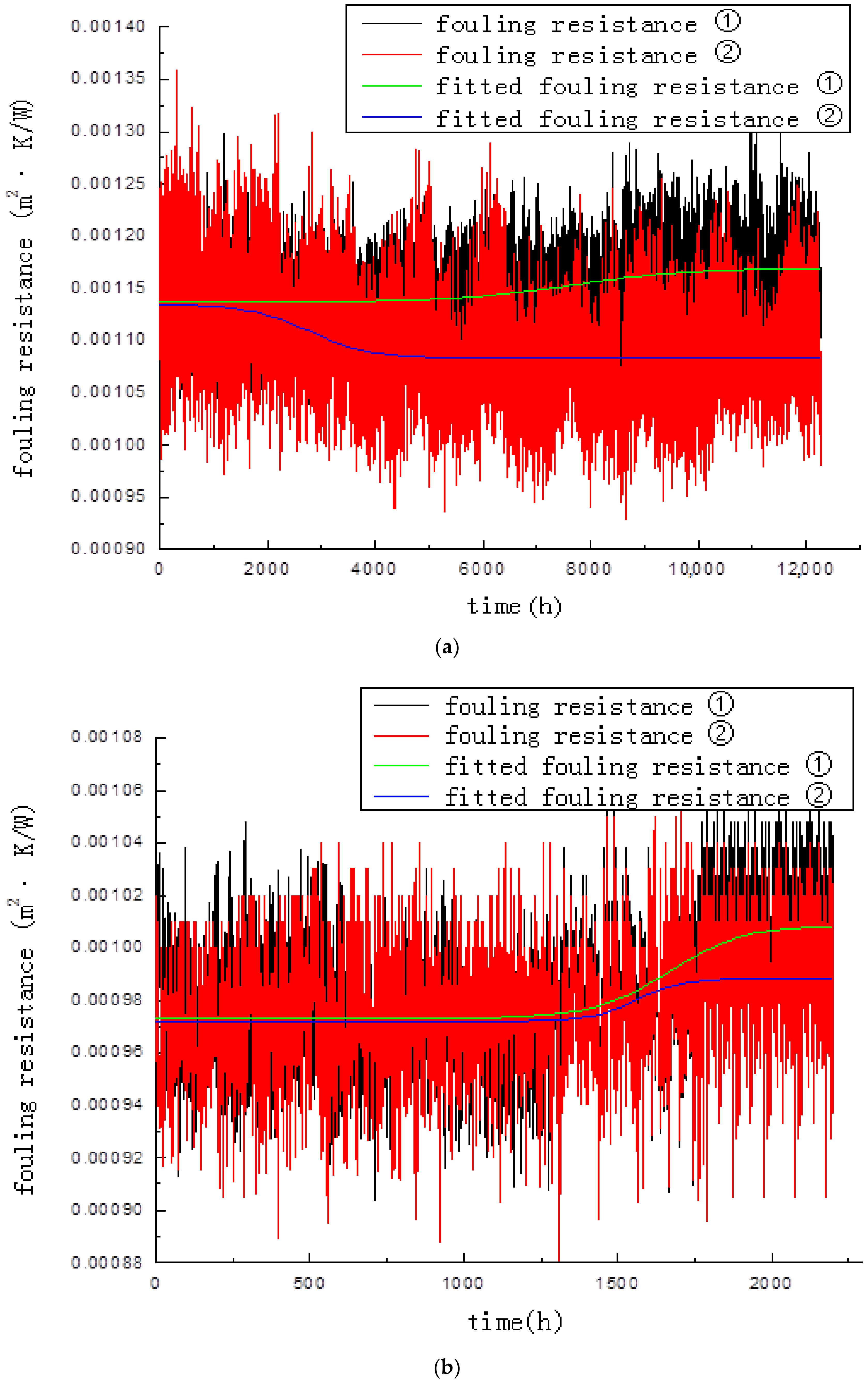
The inhibitory effect of electromagnetic fields on fouling in 1 kHz and 5 kHz magnetic and contrast experiments is shown in Figure 2. Results reveal that variations in aqueous solutions, water quality parameters, and fouling resistance in magnetic experiments tended to be different from those in contrast experiments. The fouling resistance value on the heat-exchanging surface in magnetic experiments was smaller than that in contrast experiments after the initial values returned to zero. The anti-fouling efficiency in 1 kHz and 5 kHz magnetic and contrast experiments was 91.23% and 46.97%, respectively, by calculating Equations (6) and (7). Better anti-fouling performance was realized under the influence of low-frequency electromagnetic fields. Electromagnetic water treatment technology influenced fouling formation, which is highly important. Turbidity was further introduced in 5 kHz magnetic fields and contrast experiments. Compared with the pH value and dissolved oxygen, conductivity was more suitable for establishing a mathematical model of the electromagnetic field and water quality parameters, producing the same result as that in 1 kHz magnetic fields and contrast experiments. Variations in conductivity were studied to obtain the application effect of electromagnetic fields for fouling mitigation. Conductivity can be used as an adaptive feedback control parameter for the optimum anti-fouling state. Furthermore, the turbidity, dissolved oxygen, and pH value can be researched in greater detail to reflect the inhibitory effects and mechanisms of electromagnetic fields on fouling.
5. Conclusions
A variable-frequency vertical electromagnetic field is proposed, where variations in conductivity, pH value, dissolved oxygen, and turbidity of 1 kHz and 5 kHz magnetic treatments were studied using SPSS. Origin was employed to analyze fouling resistance. This method is applicable to other experimental conditions, and several important conclusions can be drawn.
(1) The relevance of conductivity and magnetic acting time is better than that of pH value and dissolved oxygen, and conductivity is more suitable for establishing a mathematical model of electromagnetic fields and water quality parameters.
(2) Turbidity, dissolved oxygen, pH value, and fouling resistance reflect electromagnetic anti-fouling performance to different extents, contributing to the interpretation of related experimental phenomena and verification of the electromagnetic anti-fouling mechanism.
(3) The effect of the electromagnetic field on water quality parameters implies that variable-frequency electromagnetic water treatment technology is applicable in fouling mitigation. This technology improves the operating efficiency of industrial heat-transfer equipment and realizes an economic, effective, and environmental physical anti-fouling method.
Author Contributions
F.H. designed the study; J.W. analyzed the data and managed the project; F.H. wrote and revised the manuscript.
Acknowledgments
This research was supported by the Fundamental Research Funds for the Central Universities (Grant No. BLX201604), the National Natural Science Foundation of China (Grant No. 51176028), and the Natural Science Foundation of Jilin Province, China (Grant No. 201115179).
Conflicts of Interest
The authors declare no conflict of interest.
Nomenclature
| Symbols | |
| Beta standardized regression coefficient | |
| DO | dissolved oxygen (mg/L) |
| bk | kurtosis |
| P | significant level |
| r | partial correlation coefficient |
| R | correlation coefficient, [−1, 1] |
| R2 | square of correlation coefficient, [0, 1] |
| sk | skewness |
| Se | standard error of estimate |
| Sk | standard error of kurtosis |
| Ss | standard error of skewness |
| t | t-test of SPSS statistics software |
| TU | turbidity (FTU) |
| VIF | variance inflation factor |
| Greek Letters | |
| 𝜅 | conductivity (μS/cm) |
| σ | standard error |
References
- Babakhani, D. Analytical approach based on a mathematical model of an air dehumidification process. Braz. J. Chem. Eng. 2013, 30, 793–799. [Google Scholar] [CrossRef] [Green Version]
- Cho, Y.I.; Kim, W.I.; Cho, D.J. Electro-flocculation mechanism of physical water treatment for the mitigation of mineral fouling in heat exchangers. Exp. Heat Transf. 2007, 20, 323–335. [Google Scholar] [CrossRef]
- Demopoulos, G.P. Aqueous precipitation and crystallization for the production of particulate solids with desired properties. Hydrometallurgy 2009, 96, 199–214. [Google Scholar] [CrossRef]
- Wang, J.G.; Liang, Y.D. Anti-fouling effect of axial alternating electromagnetic field on calcium carbonate fouling in U-shaped circulating cooling water heat exchange tube. Int. J. Heat Mass Transf. 2017, 115, 774–781. [Google Scholar] [CrossRef]
- Wang, J.G.; He, F.; Di, H. Correlation analysis of magnetic field and conductivity, pH value in electromagnetic restraint of scale formation. CIESC J. 2012, 63, 1468–1473. [Google Scholar] [CrossRef]
- Hong, Y.X.; Deng, X.H.; Zhang, L.S. 3D numerical study on compound heat transfer enhancement of converging-diverging tubes equipped with twin twisted tapes. Chin. J. Chem. Eng. 2012, 20, 589–601. [Google Scholar] [CrossRef]
- Ji, X.S.; Xin, Q.C.; Xiang, H.Q. Multiple stepwise regression analysis of gravity dam’s deformation monitoring data based on SPSS. China Rural Water Hydropower 2012, 7, 141–143. [Google Scholar]
- Lai, G.Y.; Chen, C. Common Function and Application of SPSS 17.0, 1st ed.; Electronic Industry Press: Beijing, China, 2010; pp. 241–263. ISBN 9787121113307. [Google Scholar]
- Li, C.; Li, J.M. Laminar forced convection heat and mass transfer of humid air across a vertical plate with condensation. Chin. J. Chem. Eng. 2011, 19, 944–954. [Google Scholar] [CrossRef]
- Moussa, D.T.; El-Naas, M.H.; Nasser, M.; Al-Marri, M.J. A comprehensive review of electrocoagulation for water treatment: Potentials and challenges. J. Environ. Manag. 2017, 186, 24–41. [Google Scholar] [CrossRef] [PubMed]
- Li, T.; Feng, Z.P.; Song, W.J.; Gao, R.X. Effect of electromagnetic water treatment on water environment and metal equipment. Sci. Tech. Rev. 2012, 3, 46–48. [Google Scholar] [CrossRef]
- Wang, J.G.; Di, H.; He, F. Electromagnetic frequency influence on fouling resistance and electrical conductivity. Control Instrum. Chem. Indus. 2012, 761–764. [Google Scholar] [CrossRef]
- Wang, J.G.; Zhang, X.M.; Feng, Y. Experimental study of high frequency electromagnetic field on the mitigation of fouling effect. Control Instrum. Chem. Indus. 2010, 37, 83–85. [Google Scholar] [CrossRef]
- Wang, Y.W.; Dai, W.; Luo, X.N.; Zhan, D.Y.; Li, Z.Q.; Zhou, Y. Application of SPSS to the data processing in electromagnetism experiment course. J. Langfang Teach. Coll. (Nat. Sci. Ed.) 2012, 12, 22–25. [Google Scholar] [CrossRef]
- Li, W.; Zhang, W.; Li, G.Q.; Zhang, Z.J.; Qin, X.A.; Wang, T.K.; Xu, Z.M. Experimental research on the fouling resistant of internal helical-rib tubes. J. Eng. Thermophys. 2009, 30, 1578–1580. [Google Scholar] [CrossRef]
- Rung, H.L. A Study of Physical Water Treatment Technology to Mitigate the Mineral Fouling in a Heat Exchanger. Ph.D. Thesis, Drexel University, Philadelphia, PA, USA, 2012. [Google Scholar]
- Cheng, S.Y.; Zhou, Y.; Li, J.B.; Lang, J.L.; Wang, H.Y. A new statistical modeling and optimization framework for establishing high-resolution PM10 emission inventory—I. Stepwise regression model development and application. Atmos. Environ. 2012, 60, 613–622. [Google Scholar] [CrossRef]
- Cevik, A.; Göğüs, M.T.; GüzelbeY, I.H.; Filiz, H. A new formulation for longitudinally stiffened webs subjected to patch loading using stepwise regression method. Adv. Eng. Softw. 2010, 41, 611–618. [Google Scholar] [CrossRef]
- Mwaba, M.G.; Rindt, C.C.M.; VanSteenhoven, A.A.; Vorstman, M.A.G. Experimental investigation of CaSO4 crystallization on a flat plate. Heat Transf. Eng. 2006, 27, 48–54. [Google Scholar] [CrossRef]
- Rodriguez, C.; Smith, R. Optimization of operating conditions for mitigating fouling in heat exchanger networks. Chem. Eng. Res. Des. 2007, 85, 839–851. [Google Scholar] [CrossRef]
- Steinhagen, R.; Steinhagen, H.M.; Maani, K. Problems and costs due to heat exchanger fouling in New Zealand industries. Heat Transf. Eng. 1993, 14, 19–30. [Google Scholar] [CrossRef]
- Tian, L.; Huang, Y.; Sun, W.W.; Wang, G.Z. Discussions on Some Issues of Electromagnetic Anti-Fouling in Circulating Water Treatment Process; Thermal Power Branch of Chinese Society of Electrical Engineering: Jilin, China, 2010. [Google Scholar]
- Zhao, X. Experimental Study of Electromagnetic Frequency on Fouling Suppression Mechanism and Effect Evaluating. Master’s Thesis, Northeast Electric Power University, Jilin, China, 2010. [Google Scholar]
Figure 1.
Water treatment technology and fouling prevention and anti-corrosion effect of online evaluation experiment (research group, Jilin, China). (a) 1: Outlet temperature monitor; 2–4: Water temperature monitor; 5: Inlet temperature monitor; 6: Electric heater; 7: Flowmeter; 8: Upper tank; 9: Upper tank temperature monitor; 10: Lower tank; 11: Heat exchanger; 12: Overflow pipe; 13: Cooling water circulation pump; 14: Air-cooled radiator; 15: Air circulating pump; 16: Air-cooled tank; 17: Data acquisition card; 18: Proportion Integration Differentiation (PID)controller; 19: Industrial computer; 20: Water bath temperature monitor. (b) Structure principle of perpendicular electromagnetic field.

Figure 2.
Trend diagram of fouling resistance in the experimental process. (a) Fouling resistance in 1 kHz magnetic and contrast experiments. (b) Fouling resistance in 5 kHz magnetic and contrast experiments. ① contrast experiment data. ② magnetic experiment data.
Figure 2.
Trend diagram of fouling resistance in the experimental process. (a) Fouling resistance in 1 kHz magnetic and contrast experiments. (b) Fouling resistance in 5 kHz magnetic and contrast experiments. ① contrast experiment data. ② magnetic experiment data.


Table 1.
Parameter values in 1 kHz magnetic and contrast experiments.
| Time (h) | Difference (μs/cm) | pH① | pH② | pH Difference | DO① (mg/L) | DO② (mg/L) | DO Difference (mg/L) | ||
|---|---|---|---|---|---|---|---|---|---|
| 3 | 2419 | 2479 | 60 | 9.10 | 9.16 | 0.06 | 0.40 | 0.48 | 0.08 |
| 6 | 2402 | 2460 | 58 | 8.51 | 8.31 | −0.20 | 5.32 | 5.39 | 0.07 |
| 9 | 2424 | 2472 | 48 | 8.38 | 8.28 | −0.10 | 0.40 | 0.37 | −0.03 |
| 12 | 2441 | 2470 | 29 | 8.39 | 8.23 | −0.16 | 0.16 | 0.23 | 0.07 |
| 15 | 2463 | 2476 | 13 | 8.29 | 8.24 | −0.05 | 3.78 | 4.15 | 0.37 |
| 18 | 2423 | 2493 | 70 | 8.32 | 8.20 | −0.12 | 5.36 | 5.79 | 0.43 |
| 21 | 2422 | 2486 | 64 | 8.24 | 8.19 | −0.05 | 0.04 | 0.04 | 0.00 |
| 24 | 2416 | 2470 | 54 | 8.25 | 8.22 | −0.03 | 4.87 | 5.44 | 0.57 |
| 27 | 2437 | 2480 | 43 | 8.26 | 8.21 | −0.05 | 6.43 | 6.08 | −0.35 |
| 30 | 2425 | 2436 | 11 | 8.17 | 8.16 | −0.01 | 0.58 | 1.09 | 0.51 |
| 33 | 2417 | 2441 | 24 | 8.17 | 8.15 | −0.02 | 0.10 | 0.08 | −0.02 |
| 36 | 2438 | 2452 | 14 | 8.22 | 8.18 | −0.04 | 4.47 | 4.66 | 0.19 |
| 39 | 2430 | 2457 | 27 | 8.18 | 8.14 | −0.04 | 4.17 | 4.68 | 0.51 |
| 42 | 2452 | 2451 | −1 | 8.22 | 8.22 | 0.00 | 0.30 | 0.28 | −0.02 |
| 45 | 2422 | 2444 | 22 | 8.14 | 8.19 | 0.05 | 8.83 | 6.44 | −2.39 |
| 48 | 2467 | 2444 | −23 | 8.20 | 8.14 | −0.06 | 0.33 | 0.39 | 0.06 |
| 51 | 2461 | 2450 | −11 | 8.18 | 8.21 | 0.03 | 0.41 | 0.45 | 0.04 |
| 54 | 2435 | 2441 | 6 | 8.19 | 8.17 | −0.02 | 1.61 | 9.76 | 8.15 |
| 57 | 2450 | 2426 | −24 | 8.19 | 8.20 | 0.01 | 0.03 | 0.04 | 0.01 |
| 60 | 2433 | 2426 | −7 | 8.23 | 8.19 | −0.04 | 4.29 | 4.74 | 0.45 |
| 63 | 2456 | 2426 | −30 | 8.21 | 8.20 | −0.01 | 0.41 | 2.19 | 1.78 |
| 66 | 2433 | 2437 | 4 | 8.20 | 8.21 | 0.01 | 5.64 | 5.19 | −0.45 |
| 69 | 2433 | 2430 | −3 | 8.12 | 8.20 | 0.08 | 0.06 | 0.04 | −0.02 |
| 72 | 2441 | 2452 | 11 | 8.23 | 8.19 | −0.04 | 0.06 | 0.05 | −0.01 |
| 75 | 2448 | 2433 | −15 | 8.18 | 8.18 | 0.00 | 0.16 | 0.11 | −0.05 |
| 78 | 2440 | 2442 | 2 | 8.22 | 8.22 | 0.00 | 0.32 | 0.08 | −0.24 |
| 81 | 2438 | 2448 | 10 | 8.06 | 8.18 | 0.12 | 0.09 | 0.08 | −0.01 |
| 84 | 2459 | 2453 | −6 | 8.19 | 8.09 | −0.10 | 4.27 | 4.42 | 0.15 |
| 87 | 2448 | 2410 | −38 | 8.19 | 8.16 | −0.03 | 0.24 | 0.17 | −0.07 |
| 90 | 2454 | 2412 | −42 | 8.10 | 8.07 | −0.03 | 0.20 | 0.20 | 0.00 |
| 93 | 2459 | 2409 | −50 | 8.17 | 8.05 | −0.12 | 0.27 | 0.25 | −0.02 |
| 96 | 2430 | 2413 | −17 | 8.15 | 8.03 | −0.12 | 0.13 | 0.10 | −0.03 |
| 99 | 2433 | 2429 | −4 | 8.22 | 8.26 | 0.04 | 0.28 | 0.29 | 0.01 |
| 102 | 2432 | 2390 | −42 | 8.20 | 8.24 | 0.04 | 0.04 | 0.03 | −0.01 |
| 105 | 2431 | 2392 | −39 | 8.17 | 8.24 | 0.07 | 0.03 | 0.03 | 0.00 |
| 108 | 2452 | 2394 | −58 | 8.20 | 8.22 | 0.02 | 0.00 | 0.02 | 0.02 |
Table 2.
Parameter values in 5 kHz magnetic and contrast experiments.
| Time (h) | pH① | pH② | pH Difference | DO② (mg/L) | DO② (mg/L) | DO Difference (mg/L) | TU① (FTU) | TU② (FTU) | TU Difference (FTU) | |||
|---|---|---|---|---|---|---|---|---|---|---|---|---|
| 3 | 2434 | 2422 | −12 | 8.11 | 8.81 | 0.70 | 0.06 | 0.08 | 0.02 | 6.20 | 6.20 | 0.00 |
| 6 | 2439 | 2469 | 30 | 8.40 | 8.00 | −0.40 | 0.05 | 0.13 | 0.08 | 6.20 | 6.20 | 0.00 |
| 9 | 2395 | 2451 | 56 | 8.31 | 8.03 | −0.28 | 0.02 | 0.00 | −0.02 | 6.20 | 6.20 | 0.00 |
| 12 | 2396 | 2460 | 64 | 8.22 | 8.15 | −0.07 | 0.09 | 0.04 | −0.05 | 6.20 | 6.20 | 0.00 |
| 15 | 2303 | 2435 | 132 | 8.12 | 8.09 | −0.03 | 0.02 | 0.45 | 0.43 | 6.20 | 6.20 | 0.00 |
| 18 | 2308 | 2440 | 132 | 8.24 | 8.14 | −0.10 | 4.85 | 4.83 | −0.02 | 6.20 | 6.20 | 0.00 |
| 21 | 2312 | 2450 | 138 | 8.16 | 8.01 | −0.15 | 6.07 | 5.52 | −0.55 | 3.68 | 6.20 | 2.52 |
| 24 | 2242 | 2449 | 207 | 8.04 | 8.09 | 0.05 | 7.30 | 5.70 | −1.60 | 6.10 | 6.20 | 0.10 |
| 27 | 2253 | 2438 | 185 | 8.05 | 8.10 | 0.05 | 5.38 | 4.01 | −1.37 | 3.30 | 4.88 | 1.58 |
| 30 | 2251 | 2453 | 202 | 8.09 | 8.12 | 0.03 | 0.18 | 0.22 | 0.04 | 2.61 | 3.84 | 1.23 |
| 33 | 2263 | 2446 | 183 | 8.10 | 8.17 | 0.07 | 2.21 | 0.11 | −2.10 | 2.94 | 4.73 | 1.79 |
| 36 | 2206 | 2268 | 62 | 7.43 | 7.92 | 0.49 | 0.13 | 0.08 | −0.05 | 2.61 | 3.84 | 1.23 |
| 39 | 2216 | 2265 | 49 | 8.07 | 8.10 | 0.03 | 0.10 | 0.11 | 0.01 | 2.47 | 3.25 | 0.78 |
| 42 | 2197 | 2273 | 76 | 7.84 | 7.90 | 0.06 | 0.26 | 0.24 | −0.02 | 2.39 | 2.93 | 0.54 |
| 45 | 2204 | 2267 | 63 | 7.97 | 8.01 | 0.04 | 0.36 | 0.36 | 0.00 | 2.35 | 2.89 | 0.54 |
| 48 | 2234 | 2258 | 24 | 7.93 | 7.92 | −0.01 | 0.37 | 0.36 | −0.01 | 2.11 | 1.76 | −0.35 |
| 51 | 2194 | 2241 | 47 | 8.07 | 8.05 | −0.02 | 0.09 | 0.09 | 0.00 | 1.49 | 3.97 | 2.48 |
| 54 | 2225 | 2247 | 22 | 7.94 | 8.01 | 0.07 | 0.20 | 0.10 | −0.10 | 1.38 | 1.64 | 0.26 |
| 57 | 2206 | 2247 | 41 | 7.99 | 7.74 | −0.25 | 2.26 | 2.41 | 0.15 | 2.30 | 3.35 | 1.05 |
| 60 | 2201 | 2251 | 50 | 7.79 | 7.94 | 0.15 | 0.79 | 0.52 | −0.27 | 1.60 | 4.80 | 3.20 |
| 63 | 2242 | 2251 | 9 | 7.89 | 7.97 | 0.08 | 0.20 | 0.22 | 0.02 | 1.47 | 1.68 | 0.21 |
| 66 | 2208 | 2235 | 27 | 7.96 | 8.03 | 0.07 | 0.17 | 0.17 | 0.00 | 1.69 | 3.14 | 1.45 |
| 69 | 2204 | 2239 | 35 | 7.76 | 7.84 | 0.08 | 0.14 | 0.21 | 0.07 | 1.27 | 1.99 | 0.72 |
| 72 | 2230 | 2240 | 10 | 8.06 | 7.84 | −0.22 | 4.63 | 4.57 | −0.06 | 1.02 | 1.28 | 0.26 |
| 75 | 2214 | 2223 | 9 | 8.08 | 7.10 | −0.98 | 0.05 | 0.53 | 0.48 | 0.58 | 1.42 | 0.84 |
| 78 | 2203 | 2232 | 29 | 6.83 | 7.92 | 1.09 | 4.13 | 4.80 | 0.67 | 1.20 | 1.76 | 0.56 |
| 81 | 2192 | 2221 | 29 | 7.97 | 7.97 | 0.00 | 4.72 | 4.50 | −0.22 | 1.32 | 1.50 | 0.18 |
| 84 | 2198 | 2223 | 25 | 7.98 | 8.04 | 0.06 | 6.99 | 6.26 | −0.73 | 0.71 | 1.59 | 0.88 |
Table 3.
Descriptive analysis of variables in 1 kHz magnetic and contrast experiments.
| Min | Max | σ | sk | Ss | bk | Sk | |
|---|---|---|---|---|---|---|---|
| difference (μS/cm) | −58.000 | 70.000 | 34.150 | 0.188 | 0.393 | −0.664 | 0.768 |
| pH difference | −0.200 | 0.120 | 0.068 | −0.394 | 0.393 | 0.390 | 0.768 |
| DO difference (mg/L) | −2.390 | 8.150 | 1.459 | 4.603 | 0.393 | 25.991 | 0.768 |
Table 4.
Descriptive analysis of variables in 5 kHz magnetic and contrast experiments.
| Min | Max | σ | sk | Ss | bk | Sk | |
|---|---|---|---|---|---|---|---|
| difference (μS/cm) | −12.000 | 207.000 | 63.623 | 1.107 | 0.441 | 0.009 | 0.858 |
| pH difference | −0.980 | 1.090 | 0.351 | 0.450 | 0.441 | 4.655 | 0.858 |
| DO difference (mg/L) | −2.100 | 0.670 | 0.601 | −1.910 | 0.441 | 3.867 | 0.858 |
| TU difference(FTU) | −0.350 | 3.200 | 0.885 | 1.185 | 0.441 | 0.960 | 0.858 |
Table 5.
Summary of model in 1 kHz magnetic and contrast experiments.
| Model | R | R2 | Adjusted R2 | Se | Durbin-Watson |
|---|---|---|---|---|---|
| 1 | 0.848 | 0.719 | 0.692 | 2.718 | - |
| 2 | 0.847 | 0.718 | 0.700 | 2.681 | - |
| 3 | 0.838 | 0.702 | 0.693 | 2.715 | 1.038 |
Table 6.
Parameter estimation of model in 1 kHz magnetic and contrast experiments (part).
| Model | Variable | σ | Beta | t | p | VIF |
|---|---|---|---|---|---|---|
| 1 | Constant | 0.490 | - | 20.749 | 0.000 | - |
| difference | 0.843 | −0.801 | −8.178 | 0.000 | 1.091 | |
| pH difference | 0.422 | 0.130 | 1.321 | 0.196 | 1.094 | |
| DO difference | 0.025 | −0.031 | −0.331 | 0.743 | 1.005 | |
| 2 | Constant | 0.477 | - | 21.238 | 0.000 | - |
| difference | 0.831 | −0.800 | −8.284 | 0.000 | 1.089 | |
| pH difference | 0.415 | 0.132 | 1.364 | 0.182 | 1.089 | |
| 3 | Constant | 0.456 | - | 21.744 | 0.000 | - |
| difference | 0.806 | −0.838 | −8.942 | 0.000 | 1.000 |
Table 7.
Eliminated variables of model in 1 kHz magnetic and contrast experiments.
| Model | Excluded Variable | t | p | r | Tolerance | VIF | Min Tolerance |
|---|---|---|---|---|---|---|---|
| 2 | DO difference | −0.331 | 0.743 | −0.058 | 0.995 | 1.005 | 0.914 |
| 3 | DO difference | −0.415 | 0.681 | −0.072 | 1.000 | 1.000 | 1.000 |
| pH difference | 1.364 | 0.182 | 0.231 | 0.918 | 1.089 | 0.918 |
Table 8.
Summary of model in 5 kHz magnetic and contrast experiments.
| Model | R2 | Adjusted R2 | Variance | Durbin-Watson | ||
|---|---|---|---|---|---|---|
| Sm | F | p | ||||
| 1 | 0.329 | 0.213 | 0.329 | 2.823 | 0.048 | - |
| 2 | 0.329 | 0.245 | 0.000 | 3.920 | 0.021 | - |
| 3 | 0.315 | 0.260 | -0.014 | 5.752 | 0.009 | 0.404 |
Table 9.
Parameter estimation of model in 5 kHz magnetic and contrast experiments (part).
| Model | Variable | σ | Se | r | t | p | VIF |
|---|---|---|---|---|---|---|---|
| 1 | Constant | 1.753 | - | - | 4.726 | 0.000 | - |
| difference | 0.172 | 0.633 | 0.495 | 2.900 | 0.008 | 1.636 | |
| pH difference | 1.421 | 0.021 | 0.021 | 0.121 | 0.905 | 1.002 | |
| DO difference | 0.031 | −0.151 | −0.117 | −0.684 | 0.501 | 1.677 | |
| TU difference | 0.839 | 0.285 | 0.273 | 1.597 | 0.124 | 1.090 | |
| 2 | Constant | 1.717 | - | - | 4.829 | 0.000 | - |
| difference | 0.168 | 0.634 | 0.496 | 2.968 | 0.007 | 1.634 | |
| DO difference | 0.030 | −0.152 | -0.117 | −0.700 | 0.491 | 1.677 | |
| TU difference | 0.821 | 0.285 | 0.273 | 1.635 | 0.115 | 1.089 | |
| 3 | Constant | 1.608 | - | - | 4.914 | 0.000 | - |
| difference | 0.134 | 0.545 | 0.531 | 3.208 | 0.004 | 1.055 | |
| TU difference | 0.800 | 0.307 | 0.299 | 1.806 | 0.083 | 1.055 |
© 2018 by the authors. Licensee MDPI, Basel, Switzerland. This article is an open access article distributed under the terms and conditions of the Creative Commons Attribution (CC BY) license (http://creativecommons.org/licenses/by/4.0/).
Share and Cite
MDPI and ACS Style
He, F.; Wang, J. Statistical Analysis of Circulating Water Quality Parameters under Variable-Frequency Vertical Electromagnetic Fields. Processes 2018, 6, 182. https://doi.org/10.3390/pr6100182
AMA Style
He F, Wang J. Statistical Analysis of Circulating Water Quality Parameters under Variable-Frequency Vertical Electromagnetic Fields. Processes. 2018; 6(10):182. https://doi.org/10.3390/pr6100182
Chicago/Turabian StyleHe, Fang, and Jianguo Wang. 2018. "Statistical Analysis of Circulating Water Quality Parameters under Variable-Frequency Vertical Electromagnetic Fields" Processes 6, no. 10: 182. https://doi.org/10.3390/pr6100182
Note that from the first issue of 2016, this journal uses article numbers instead of page numbers. See further details here.