Abstract
Bioprocesses for the production of renewable energies and materials lack efficient separation processes for the utilized microorganisms such as algae and yeasts. Dissolved air flotation (DAF) and microflotation are promising approaches to overcome this problem. The efficiency of these processes depends on the ability of microorganisms to aggregate with microbubbles in the flotation tank. In this study, different new or adapted aggregation models for microbubbles and microorganisms are compared and investigated for their range of suitability to predict the separation efficiency of microorganisms from fermentation broths. The complexity of the heteroaggregation models range from an algebraic model to a 2D population balance model (PBM) including the formation of clusters containing several bubbles and microorganisms. The effect of bubble and cell size distributions on the flotation efficiency is considered by applying PBMs, as well. To determine the sensitivity of the results on the model assumptions, the modeling approaches are compared, and suggestions for their range of applicability are given. Evaluating the computational fluid dynamics (CFD) of a dissolved air flotation (DAF) system shows the heterogeneity of the fluid dynamics in the flotation tank. Since analysis of the streamlines of the tank show negligible back mixing, the proposed aggregation models are coupled to the CFD data by applying a Lagrangian approach.
1. Introduction
Yeast cells and algae are frequently used in bioprocesses for the production of renewable materials and biofuels such as bioplastic precursors [1], bioethanol [2], and biodiesel [3,4]. The separation of the microorganisms after fermentation is capital and energy intensive. The high separation costs are caused by the small size of microorganisms and their density being close to water [5]. Additionally, especially microalgae grow in very dilute cultures [6,7]. Thus, traditional filtration, sedimentation and centrifugation techniques are inefficient [8]. The development of efficient industrial-scale separation processes is essential for the economically-feasible production of renewable materials and biofuels. High speed centrifugation methods such as disc stack centrifuges result in high forces, which may result in the breakup of microorganisms [9]. Based on the separation performance and energy consumption criteria, hydrocyclones are an alternative to separate microorganisms in the size range of m [10]. Hydrocyclones have a small footprint and relatively low capital and operating costs [11]. Recent studies showed the potential of hydrocyclones to separate yeast cells [12,13] from fermentation broths. However, the single-stage efficiencies of hydrocyclones may be low for particles smaller than m. The diameter of hydrocyclones determines largely the particle-cut size (size at which the partition number equals 0.5) and throughput. For particle separation in the micron range, small diameter hydrocyclones (about 10–100 mm) with small throughputs have to be used [11]. For large-scale plants, an extreme numbering-up would be necessary when separating microorganisms with mini-hydrocyclones. That would result in high capital costs. Promising approaches to separate microorganisms from broth are dissolved air flotation (DAF) [7,14] and microflotation [15,16]. In both flotation principles, microbubbles (bubbles with diameter ranging from 10 to 100 µm) are generated at the inlet to a flotation tank [15,17]. In the flotation tank, the microbubbles and particles aggregate. The particle-bubble aggregates either float into the froth of the tank or are entrained within the clear or recycle stream [18,19]. The removal of microorganisms requires a hydrophobic surface, which might require usage of an appropriate surfactant [20]. DAF is already a widely-used separation technique in water and wastewater treatment dealing with the removal of cells or algae [3,18], particles and off-flavors [21] and flocs of organic or inorganic materials [22] from water. In order to yield high separation efficiencies, a pre-flocculation process with coagulants such as metallic salts, polymers, cetyl trimethyl ammonium bromide and chitosan can be favorable for the separation of algae [23]. However, to avoid product damage or contamination, flocculation with coagulant should be avoided in some processes [3].
Applying suitable modeling approaches can significantly reduce the effort of determining efficient plant configurations and process conditions for flotation. The efficiency of the separation process of microorganisms with DAF or microflotation depends on the ability of microorganisms to aggregate with microbubbles. To our knowledge, there exists no generic and physically correct modeling approach for this heteroaggregation process. Only Zhang et al. [20] modeled the harvesting of microorganisms with DAF by applying the so-called “White Water Blanket Model”. They consider the aggregation of several bubbles on single flocs of cells, which are polydisperse in size. However, they neglected the polydispersity of bubbles and the formation of clusters consisting of several bubbles and flocs. In the present study, several mechanistic approaches are taken to model the heteroaggregation between microorganisms and microbubbles in flotation tanks. While still being adapted to the given problem, some of the aggregation models are based on existing models for particle separation by DAF (models where multiple monodisperse bubbles can aggregate on larger monodisperse particles [22,24,25], models where smaller monodisperse bubbles aggregate on larger polydisperse particles [19,26] and a model where multiple monodisperse bubbles and cells form clusters [27]). Other modeling approaches are newly developed in this study. The default assumptions are that the cells and bubbles are monodisperse and the loading of cells on bubbles is distributed, i.e., non-identical. Each of the six models is based on different assumptions for the flotations system: (1) averaged, i.e., identical, loading of cells on bubbles, (2) distributed, i.e., non-identical, loading of cells on bubbles, (3) polydispersity of cells, (4) polydispersity of bubbles and the formation of clusters, (5) without and (6) with an averaged, i.e., identical, number of cells and bubbles. We did not consider both bubbles and cell sizes to be polydisperse in the same model. Such a consideration would lead to a two-dimensional population balance model. For such a model, the direct use of commercial codes, the coupling to CFD simulations and experimental validation become much more difficult, while it is not clear yet whether this provides a significant benefit. Restricting the model choices to ordinary differential and one-dimensional population balance equations allows easier use of the model and simplifies experimental validation. Because only the models including the polydispersity of bubbles can consider bubble coalescence, bubble coalescence is neglected, but modeling it is possible [28]. Furthermore, measurements of bubble size distributions during microflotation in complex fermentation broths have been performed and showed that the presence of proteins of YMP hinders bubble coalescence [29]. Thus, parametrization and validation of this submodel are possible. To determine the sensitivity of the results on the presented assumptions, the models are compared and suggestions for applicability are given. The Computational fluid dynamics (CFD) data of a DAF system shows that the fluid dynamics are highly heterogeneous in the flotation tank and that there is negligible back mixing. Thus, the aggregation models are coupled with the CFD data of the DAF system by using a Lagrangian approach.
2. Modeling Approaches
In this study, six different mechanistic models for the heteroaggregation between microbubbles and microorganisms dispersed in a fluid are investigated to calculate the separation efficiency of microorganisms in flotation systems. The aggregation models exhibit different levels of complexity. Two approaches to model the floatation tank are used for each aggregation model: the classical two-zone model [18] with constant flow conditions and the coupling to CFD data [30].
2.1. Aggregation Kernel
Each aggregation model contains the aggregation kernel . The aggregation kernel for the aggregation mechanism i is a combination of the encounter frequency and the encounter efficiency, which is the probability of an encounter leading to a successful collision [27]:
where and are the encounter efficiencies due to physiochemical and hydrodynamic effects, respectively. Commonly, the kernels for different mechanisms are superimposed [27,30]:
where , and are the aggregation kernels due to laminar shear, sedimentation and turbulent motion. Here, aggregation due to Brownian motion can be neglected, since the cells and bubbles are too large to observe Brownian motion [31]. It is well known [32,33] that an error is made with the linear superimposition, but no closed form including all of the relevant mechanisms exists yet. Furthermore, as the focus of this study is on comparing different models, a perfect representation of the kernels is not necessary. Substituting Equation (1) in Equation (2) and assuming that the physiochemical encounter efficiency is independent of the aggregation mechanism, the following relation is obtained:
2.1.1. Frequency of Encounters
The frequency of encounters is calculated for each mechanism: laminar shear, sedimentation and turbulent motion. Pedocchi and Piedra-Cueva [34] have extended the frequency of encounters due to laminar shear by von Smoluchowski [35] from a one-dimensional formulation to a three-dimensional one (Equation (Table 1) in Table 1), where u, v and w are the fluid velocities in the x, y and z directions. To calculate the encounter frequency due to density differences between two different aggregates, Equation (Table 1) in Table 1 has been used [27], where and are the rising or settling velocities of the two aggregates 1 and 2. The rising velocity of aggregates consisting of bubbles is set to the rising velocity of single bubbles. For the turbulent encounter frequency, the Saffman–Turner relation is used [32] (Equation (Table 1) in Table 1).

Table 1.
Encounter frequencies and efficiencies used for aggregation kernels.
2.1.2. Encounter Efficiency
The hydrodynamic encounter efficiency considers the fact that the flow field around the bubble and particle hinders aggregation [36,37]. can be expressed as Equation (14) in Table 1, where and are the diameter of the particle and bubble, is the kinematic viscosity of the fluid and is the gas volume fraction. This efficiency was derived for dirty interfaces [36,37], which is valid here, because the flotation bubbles are created in a complex medium that will make the interface dirty shortly after bubble creation. This correlation used for neglects, e.g., the effects of density differences [38], but again, the focus is not a perfect representation of the kernels, but a model comparison. The characteristic velocity U depends on the aggregation mechanism. According to Kostoglou et al. [30] and Dai et al. [39], the characteristic velocities for laminar shear and sedimentation are the rising velocities of the bubbles. The average relative velocity due to turbulent motion can be expressed as [30]:
where is the turbulent dissipation.
The encounter efficiency allows describing space limitations on the bubble [19,26] or other effects such as repulsion and attractive forces [40]. Repulsion and attractive forces depend heavily on the process conditions and can be influenced by the addition of chemicals that tailor surface properties of cells or bubbles. They can either be modeled using the DLVO theory extended by Born repulsion forces [41], or be computed using molecular dynamics simulations [42], which requires knowledge of the surface of the particles, or be measured using atomic force microscopy [43]. Recently, Ditscherlein et al. [44] introduced a new AFM method to quantify the micro-sized bubble-yeast interactions depending on the conditions of the surrounding medium such as pH, ethanol and salt concentration Using those methods to infer , the effect of chemical addition on separation efficiency should become predictable with a suitable aggregation model. Nevertheless, most of the studies on DAF estimate from empirical relations or by fitting experimental data [22,26]. Since this study describes the generalized modeling of flotation processes, is set to one. Most studies on DAF processes, including this one, consider that surface coverage reduces the encounter efficiency and assume that the encounter efficiency is proportional to the ratio of the remaining free surface to the total surface. The cells occupy their projected surface area on the bubble surface [19,22,26]. The development of layers with multiple cells on the surface of bubbles is neglected in this study, since it is assumed that the cells do weakly aggregate with others. If the cells would aggregate, one could easily use a coagulation unit prior to flotation to increase the size of the cell-aggregates and the flotation efficiency.
2.2. Spatial Models
There exist two different approaches to model the separation efficiency in DAF tanks. The traditional approach divides the DAF tank into the contact zone and the separation zone [17,18,19,26]. More advanced approaches combine CFD simulations with the aggregation process in flotation tanks [27,30,45]. In this study, both approaches are examined and applied to the different aggregation models.
2.2.1. Two-Zone Model
It is assumed that aggregation only occurs in the contact zone, where bubbles and cells enter the inlet and aggregate until the outlet of the contact zone. Since plug flow with constant flow conditions is assumed, the introduced substantial derivatives for the aggregation models in Section 2.3 simplify to time derivatives. The terms for the change of the bubble concentration over time due to velocity differences between bubbles and the fluid can be neglected. Furthermore, no aggregation occurs in the flotation zone, and all cells, which have been attached onto bubbles in the contact zone float, are thus removed. The separation efficiency is calculated as:
where and are the concentrations of unbounded cells at the outlet and at the inlet of the contact zone, respectively.
2.2.2. One-Way Coupling
To combine CFD simulations with the aggregation process in DAF tanks, first an Euler/Euler CFD simulation has been performed to obtain the flow field. In this simulation, the loading of cells on bubbles is constant, and the presence of cells is neglected for computing the fluid properties. Then, the cell number concentration on a representative stream line with a changing load of cells on bubbles is computed in a Lagrangian framework (see Section 2.3 and Section 3) using the flow conditions from the Euler/Euler simulation. Thus, the CFD result affects the cell number concentration, but the presence of cells has no influence on the CFD results. Thus, we consider a one-way coupling with regard to the cell number concentration. The Euler/Euler CFD simulation (for the commercially available DAF system Enviplan: AQUATECTOR®Microfloat®, see Figure 1a) for a two-phase system consisting of the liquid and gaseous phase has been performed with Ansys Fluent. The gaseous phase was described by bubbles with a diameter of 40 µm and a density of an air bubble with a maximum loading of microorganisms (18.28 kg/m3). Those estimates were based on experimental data for the flotation of yeasts [29]. For the liquid phase, water properties were applied. The central inlet was a mass flow inlet, the free surface a degassing boundary and one bottom opening (side) a pressure outlet. The mesh consisted of hexahedral cells (approximately 0.5 Mio.elements, which Buffo [46] (p. 129) found to be a sufficient mesh density for mesh independent results for a column with bubbly flow. Furthermore, Hecht et al. [47] observed agreement with experimental data using a similar mesh density for a column with bubbly flow). Most of the tank was expected to be laminar, while the inlet region had a Reynolds number in the turbulent regime. Therefore, different turbulence models (k-omega SST, k-epsilon) and a model without turbulence (laminar) were evaluated, but no effect on gas hold-up or flow field was observed. For drag on the bubbles, the commonly-used model by Tomiyama et al. [48] for slightly contaminated interfaces was used. Even though using a different drag model is expected to change the results of the CFD simulation slightly, this will affect all investigated models in this study in the same manner. Thus, for the main aim of model comparison, no significant changes are to be expected.
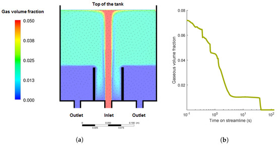
Figure 1.
Process conditions of the investigated flotation tank. (a) Gas volume fraction and velocity directions of fluid; (b) evolution of the gas volume fraction of a single streamline.
In order to combine CFD results and aggregation processes, several streamlines are tracked. While unbounded cells are assumed to follow the fluid streamline until the outlet is reached, the concentration of bubbles decreases on the course of a streamline due to velocity differences between bubbles and the fluid. This is included in the formulation of the aggregation models in Section 2.3 by substantial derivatives and the included terms for the time-dependent change of the bubble concentration. The change of the bubble concentration is combined with the CFD simulations. CFD results also show that unloaded bubbles and loaded bubbles behave very similarly. Thus, it is assumed that free bubbles and bubble-particle aggregates behave in the same way.
Additionally, CFD data show that the gas volume fraction in the outlet of the flotation tank is negligible (see Figure 1). Assuming that bubble-cell aggregates behave like unloaded bubbles, all cells, which are attached to bubbles, float. Only the unbounded cells remaining in the outlet do not float. Thus, the separation efficiency for the one-way coupling to CFD is calculated as described in Equation (16). The recycling of the outlet is generally implementable in the introduced models, but not included in the given study. The integration of heteroaggregation processes and CFD data by the realized one-way coupling poses a sufficient and useful method for design evaluation. Full coupling can be done in a future step and might be interesting if bubble dynamics might be affected by a significant change in bubble density and corresponding effects on fluid dynamics.
2.3. Heteroaggregation Modeling
In this section, the applied models for the heteroaggregation between microbubbles and cells (Figure 2) are described.
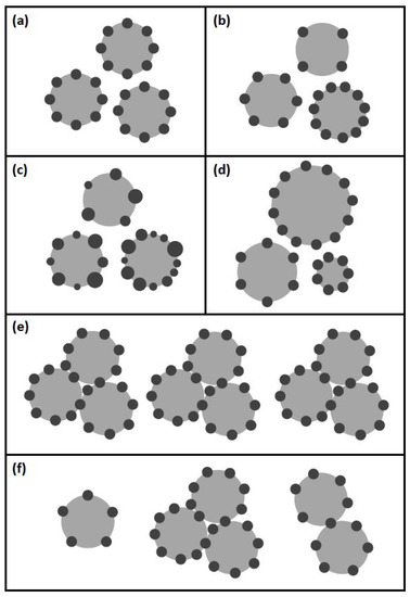
Figure 2.
Illustration of the different aggregation models, where grey spheres represent bubbles and dark spheres correspond to microorganisms: (a) Averaged: several monodisperse cells aggregate on monodisperse bubbles; loading of bubbles is averaged; (b) Not Averaged: several monodisperse cells aggregate on monodisperse bubbles; loading of bubbles is distributed; (c) Poly.Cells: several polydisperse cells aggregate on monodisperse bubbles; (d) Poly.Bubbles: several monodisperse cells aggregate on polydisperse bubbles; (e) Clustering Averaged: formation of aggregates with multiple monodisperse bubbles and monodisperse cells; bubble and cell number per cluster are averaged; (f) Clustering: formation of aggregates with multiple monodisperse bubbles and monodisperse cells; bubble and cell number per cluster are distributed.
2.3.1. Averaged
The model Averaged describes the aggregation of multiple cells on larger bubbles. Moreover, the bubbles and cells are assumed to be monodisperse in their size and shape. The loading of bubbles with cells is assumed to be uniform, i.e., each bubble’s surface area is occupied with cells in the same manner. The general equation for aggregation between cells and bubbles is:
where and are the number concentrations of unbounded cells, respectively bubbles, t is the time,and and are the diameter of the cells and bubbles, respectively. If the conditions are not homogeneous throughout the tank, that causes a dependence of the aggregation kernel on the position . The encounter efficiency due to surface coverage is calculated by Equation (7) in Table 1, where l is the ratio of the occupied and total surface area of a bubble. Applying the one-way coupling, the velocity difference between bubbles and the fluid causes a change of the bubble concentration on the course of a streamline:
where the gas volume fraction and its time-dependent change was obtained from CFD data in this study.
2.3.2. Not Averaged
In contrast to the model Averaged, the loading of bubbles with cells is not assumed to be uniform in the model Not Averaged, i.e., there exists a number density distribution of bubbles loaded with a different amount of cells. Therefore, models where multiple bubbles can aggregate on larger particles [22,24,25] have been adapted to a population balance model for the aggregation of several cells on larger bubbles. Thus, a bubble with j attached cells can be formed by the aggregation between a bubble with attached cells and a single cell. If a bubble with j attached cells aggregates with one more cell, a bubble with cells is created. The model results in a 1D discrete population balance model, in which bubbles are loaded with a discrete number of cells.
where is the number concentration of unbounded cells and is the number density of monodisperse bubbles loaded with j cells. The physiochemical collision efficiency , for a bubble already having j attached cells (compare with [26]), can be expressed as Equation (8) in Table 1, where is the maximum number of cells that can attach to a bubble.
2.3.3. Poly.Cells
In the model Poly.Cells, the bubbles are still assumed to be monodisperse, whereas cells are polydisperse in size. Since cells are polydisperse, the surface coverage of bubbles is continuous. Thus, bubbles have the occupancy level l, which is the ratio between the occupied and total surface area of a bubble. Each cell diameter is assigned a specific occupancy potential p, which can be expressed as:
where is the projected surface area of a cell and is the surface area of a bubble. Due to an aggregation with a cell with the occupancy potential p, the occupancy level of a bubble increases from to . The set of equations for the 1D continuous population balance model is:
where is the number density of polydisperse cells with the occupancy potential p and is the number density of monodisperse bubbles with the occupancy level l. is described in Equation (9) in Table 1.
2.3.4. Poly.Bubbles
The models by Fukushi et al. [19] and Matsui et al. [26] have been adapted to the heteroaggregation between smaller monodisperse cells on larger polydisperse bubbles. That results in a population balance, in which the discrete property is the loading of cells on bubbles, and the continuous property is the size of bubbles:
where is the number density of bubbles with the diameter and j attached cells. The number concentration of unbounded cells is represented as . The maximum number of cells that can attach to a single bubble depends on the respective bubble diameter. The minimum and maximum bubble diameters are defined as and . The encounter efficiency due to surface coverage is calculated as in Equation (10) in Table 1.
2.3.5. Clustering
The model Clustering is based on the model by Lakghomi et al. [27], in which clusters of bubbles and particles were considered. In this study, clustering is the formation of aggregates with multiple bubbles and cells, where both bubbles and cells are assumed to be monodisperse. This results in a discrete bivariate population balance model:
where is the number density of clusters with i bubbles and j cells. Contrary to Lakghomi et al. [27], in this study, the reduction of the encounter efficiency due to surface coverage is included. It is assumed that aggregation between two clusters can only occur, if a cell on the exposed surface of a cluster collides with a bubble on the exposed surface of the other cluster or vice versa. Then, between a cluster with i bubbles and j cells (Cluster 1) and a cluster with m bubbles and l cells (Cluster 2) can be expressed as described in Equation (11) in Table 1. and are the fractions of the exposed cluster surface area of Cluster 1, which is occupied by cells and bubbles, respectively. The derivations for and are described in the Appendix B.
There is no suitable approach to model the hydrodynamic encounter efficiency between two clusters consisting of bubbles and particles in the literature. Thus, the hydrodynamic encounter efficiency for the case of clustering has been simplified. The expression by Kostoglou et al. [30] is used for the hydrodynamic encounter efficiency of single cells and clusters consisting of one or more bubbles. For two clusters, both containing one ore more bubbles, the hydrodynamic encounter efficiency is predicted to be close to one by this model. Therefore, a value of one is used for .
2.3.6. Clustering Averaged
For the model Clustering Averaged, it is assumed that all clusters have the same number of bubbles and cells. The number concentration of free cells decreases over time due to aggregation with clusters, whereas the number concentration of clusters decreases due to the aggregation of two clusters and due to the velocity difference between bubbles and the fluid. The average number of bubbles and cells per cluster i and j can be described, as well. The product of and i only changes due to the velocity difference between bubbles and the fluid, whereas the product of and j additionally increases due to the aggregation of unbounded cells. The initial number concentration of clusters is equal to the initial bubble number concentration.
The encounter efficiency due to surface coverage between two identical cluster or between a cluster and an unbounded cell can be calculated with Equations (12) and (13) in Table 1. Equivalent to the model Clustering, Equation (14) is used for the hydrodynamic encounter efficiency of single cells and clusters consisting of one ore more bubbles. For two identical clusters, the hydrodynamic collision efficiency is close to one and therefore set to one.
3. Numerical Methods
In this study, all ODEs are solved with the MATLAB solver ode45. The models Averaged, Not Averaged and Clustering Averaged consist of a set of ordinary differential equations (ODEs). For the model Poly.Bubbles, the bubbles are classified into discrete bubble sizes. The bubbles are loaded with a discrete number of cells, which results in a discrete set of ODEs. To solve the model Poly.Cells, the cells are classified into a discrete number of cells. The loading of the bubbles is classified into discrete occupancy levels. Due to the aggregation of a bubble with a cell, the new occupancy level of the bubble is in between two discrete classes for the occupancy level. Therefore, the new built aggregates have to be divided onto neighboring nodes. For this purpose, the cell average technique is used [49] to obtain a discrete set of ODEs. In order to test for grid convergence, simulations were also performed with a finer resolution, and no difference in the results was observed. To obtain a discrete number of ODEs for the model Clustering, the maximum numbers of bubbles and cells for a cluster are limited to a discrete number. If the aggregation between two clusters would form a cluster, which would be outside of this limiting region, the aggregation process is set to be impossible. The maximum numbers of bubbles and cells for a cluster are chosen sufficiently high, i.e., the formation of clusters beyond the limiting region is rare (data not shown). Applying lower tolerances for the ODE solver than used in this study did not change the results.
4. Results and Discussion
First, the impact of the assumptions of the different aggregation models and the effects leading to the formation of clusters were investigated assuming a two-zone model. Then, the focus was set on the spatial aggregation in a commercially available DAF system (Enviplan: AQUATECTOR®Microfloat® Rundzelle). To compare different simulations, a set of standard parameters (Table 2) was introduced. The parameters have been used for the simulations, unless other parameter settings are mentioned. The turbulence dissipation rate and the shear rate were chosen in a range as observed at the inlet of the investigated flotation tank. The residence time was chosen arbitrarily, whereas the other standard parameters were set to reasonable values.
Table 2.
Standard parameters for simulations.
4.1. Comparison of the Different Aggregation Models
In this section, the heteroaggregation models are compared, whereby a plug flow was assumed, i.e., flow conditions stayed constant during the simulation. For constant flow conditions, the model Averaged had an analytical solution, which is derived in the Appendix A. The analytical solution included the dimensionless groups and :
where is the initial number concentration of cells, the initial bubble concentration, the residence time in the contact zone and the aggregation kernel for cells and unloaded bubbles. is the fraction of the initial bubble surface area that can be theoretically occupied by the cells assuming the most favorable aggregation conditions. A high aggregation number corresponds to frequent aggregation. For the standard parameter settings, and .
The separation efficiencies of the heteroaggregation models were calculated with Equation (16) and plotted over the two dimensionless groups and (Figure 3). If , the efficiency was zero, because no aggregation could occur. Then, the efficiency increased with an increasing aggregation number, since a high aggregation number resulted from favorable collision conditions. A high resulted from a high ratio between the projected surface of all cells and the surface of all bubbles. Thus, the efficiency decreased with an increasing . To calculate the separation efficiency as described in Equation (16), has to be chosen . For very small values of , the separation efficiencies of the different models already showed differences.
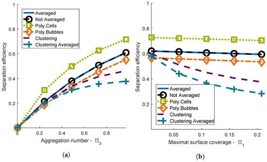
Figure 3.
Comparison between the different aggregation models (Poly.Cells: ; Poly.Bubbles: ). (a) Separation efficiency depending on the aggregation number at ; (b) separation efficiency depending on maximal surface coverage at .
No difference between the models Averaged and Not Averaged could be observed in the entire range of the dimensionless groups and . It could be observed that the loading of the bubbles for the model Averaged was approximately equal to the mean loading of bubbles for the model Not Averaged (data not shown).
The cell size distribution of microorganisms can be described by a gamma distribution [50], which allows setting the mean value and the standard deviation and guarantees positive diameters. Thus, in the model Poly.Cells, the initial cell size distribution was set to a gamma distribution. In our model, the mean diameter was equal to the standard parameter m, and the relative standard deviation was . The efficiency of the model Poly.Cells was higher than the efficiency of the model Averaged in the entire range of and , which is discussed in detail in the next section. Additionally, the difference between the two models tended to increase with higher relative standard deviations of the cell diameter (data not shown. For the model Poly.Cells, the initial bubble size distribution was assumed to be a gamma distribution with the mean diameter equal to the standard parameter m and . The efficiency of the model with polydisperse bubbles was lower than the efficiency of the model Averaged for the entire ranges of the dimensionless groups and . A possible explanation for this observation was that most of the bubbles’ volume was represented in larger bubble sizes, since the volume of a single bubble was proportional to the bubble diameter cubed. However, large bubbles were less efficient in floating cells than small bubbles [18]. The ratio between the surface and the volume of a bubble decreased with an increasing bubble diameter. This resulted in an increased maximal surface coverage and a decreased flotation efficiency for larger bubbles.
The lower the standard deviations of the models Poly.Cells and Poly.Bubbles, the more similar were the results compared to the model Averaged (data not shown).
The separation efficiencies of the models Clustering and Clustering Averaged were lower than the separation efficiencies of the model Averaged in the whole range of and . Additionally, the model Clustering Averaged yielded lower separation efficiencies than the model Clustering. This could have been caused by an overestimation of the cluster formation for the model Clustering Averaged. In general, clustering reduces the efficiency because the formation of clusters with multiple bubbles reduces the available surface area of bubbles. Therefore, the frequency of the attachment of cells decreases.
4.1.1. Influence of the Cell Size Distribution
To investigate the influence of a distributed cell diameter on the efficiency of the flotation process, the number density distribution of unbounded cells was computed at different simulation times (see Figure 4) for the model Poly.Cells. The applied relative standard deviation was . Each distribution below the initial distribution signified a subsequent simulation time. Due to aggregation with bubbles, the number density distribution of free cells decreased with an increasing simulation time. Furthermore, the number density of bigger cells decreased significantly faster than the number densities of smaller cells. Since the mass of a single cell is proportional to the cell diameter cubed, most of the mass of the cells is represented in larger cell sizes and aggregates quite fast. Therefore, the efficiency increased using a gamma distribution for the cell diameter, as can be observed in Figure 3.
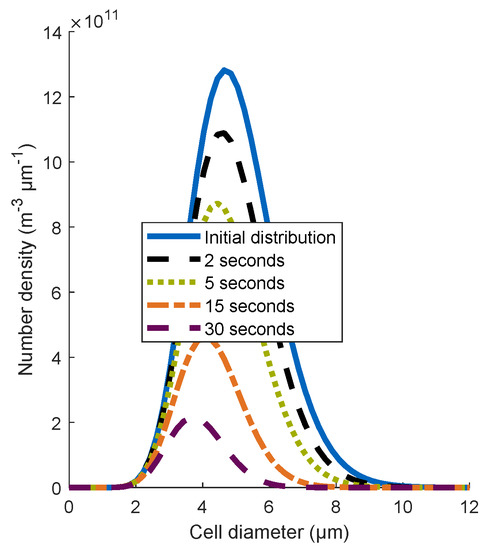
Figure 4.
Number density distribution of unbounded cells for the model Poly.Cells at different simulation times; standard parameter are used, and .
4.1.2. Mechanisms Leading to the Formation of Clusters
To detect the main effects influencing the formation of aggregates with multiple bubbles, the influence of the flow conditions were investigated. The turbulent dissipation rate and the shear rate were varied, while the dimensionless groups and were kept constant (see Figure 5a). Thus, the aggregation mechanisms due to laminar shear and turbulent motion were varied. The turbulent dissipation rate and the shear rate were plotted depending on their standard parameters and . Since and were kept constant, the efficiency for the analytical model did not change over the entire parameter range. In absence of shear and turbulence , the separation efficiencies of the models Clustering and Averaged were equal. With increasing and , the efficiency of the Clustering model decreased significantly. Figure 5b illustrates two number density distributions of clusters with a certain bubble number at a residence time of 10 s. Therein, the green dots represent the simulation of the model Clustering with no turbulence and no shear, i.e., and . The orange dots represent the simulation with the standard parameters for and . In the case of no turbulence and no shear, it can be observed that there were almost no aggregates consisting of more than one bubble. The aggregation mechanism was only due to sedimentation. This aggregation mechanism did not seem to cause clustering of aggregates with multiple bubbles significantly. On the contrary, for high turbulence and high shear, aggregates consisting of several bubbles were formed. This lowered the efficiency, since the available surface of bubbles decreased, where cells could aggregate. It can be deduced that shear and turbulence caused clustering.
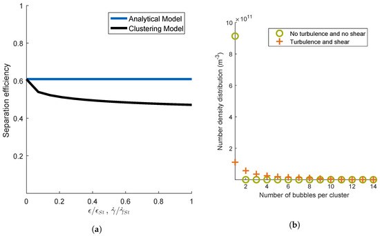
Figure 5.
Investigation on the effect of the variation of turbulent eddy dissipation and shear rate for constant and on cluster formation. (a) Separation efficiency; (b) number density distribution of clusters for the two extreme cases.
4.1.3. Scope of Aggregation Models
The properties and scopes for the different aggregation models are illustrated in Table 3. Due to comparable modeling approaches, the separation efficiencies for the aggregation models were identical for the case of monodisperse cells and bubbles and without turbulence and laminar shear (data not shown). Considering effects like clustering or a cell and bubble size distribution increased the power of the aggregation model, but also the simulation time. If cell and bubble sizes showed small standard deviations, the models Averaged, Not Averaged, Clustering and Clustering Averaged could be used for model-based optimization. Generally, the model Averaged should be preferred over the model Not Averaged for determining efficient plant configurations and process conditions, since it requires much less computational and modeling efforts and yields the same results. Since the polydispersity of cells and bubbles influences the efficiency, cell and bubble diameter distributions should be considered for quite high standard deviations by using the models Poly.Cells or Poly.Bubbles. Turbulence and laminar shear cause the formation of clusters, which lowers the flotation efficiency. Due to the low simulation time and complexity, the model Clustering Averaged may be preferred over the model Clustering for direct coupling to CFD, if turbulence and laminar shear are sufficiently high to require consideration of cluster formation. The two clustering models are also applicable if the cells exist as aggregates, which are bigger than the microbubbles.
Table 3.
Properties and scopes of aggregation models.
4.2. One-Way Coupling
In this section, the aggregation models are coupled with Euler/Euler CFD simulations for the commercially available DAF system from Enviplan (AQUATECTOR®Microfloat®) with a flow rate of 75 L/h. The geometry and the distribution of the gas volume fraction of the tank are illustrated in Figure 1a. From the inlet to the top of the tank, the gas volume fraction was quite high in a narrow area, which was the main stream of the tank. At the top of the tank, most of the bubbles remained in the foam. The other areas of the tank did not have such a high gas volume fraction. Close to the outlet, was zero. Exemplarily, the heteroaggregation on one streamline of the DAF tank was investigated in detail.
4.2.1. Gas Volume Fraction
The investigated streamline had a residence time of about 140 s. The development of the gas volume fraction is illustrated in Figure 1b. Examining the coordinates of the CFD data (not illustrated here) shows that the top of the tank was reached in about 1.5 s. After approximately 3 s, the streamline left the top of the tank and flowed to the outlet. During this time, dropped from 0.07 to 0.01. At the lower part of the tank, was zero. With the assumption that bubble-cell aggregates behave like unloaded bubbles, all cells, which were attached to bubbles, floated. Only the unbound cells remaining in the outlet did not float and were washed out of the tank.
4.2.2. Aggregation Mechanisms
The aggregation kernel of unloaded bubbles and free cells is illustrated as a function of time on the investigated streamline in Figure 6a.
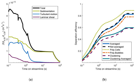
Figure 6.
Aggregation mechanisms on a single streamline and resulting separation efficiencies for different aggregation models for this streamline. (a) Importance of aggregation mechanisms on a single streamline; (b) separation efficiencies for different aggregation models.
The total aggregation kernel for the streamline was high in the first 3 s. Then, it stayed nearly constant until approximately 40 s. Between 40 and 90 s, decreased. Then, close to the outlet, increased again. During the first 2 s, the aggregation due to turbulent motion and laminar shear had a noticeable influence on the total aggregation kernel. Afterwards, sedimentation was the only important aggregation mechanism. The aggregation kernel depends on the hydrodynamic encounter efficiency, which depends on the gas volume fraction. Therefore, when the gas volume fraction decreased after 40 s, the aggregation kernel decreased as well. During the last 50 s (not shown here), the aggregation kernel increased again, since the fluid velocity increased in the region of the outlet. However, this part was not important for the aggregation process, since in this region, the gas volume fraction was already zero, and no aggregation between bubbles and cells could occur. The results for other streamlines (data not shown) were similar.
4.2.3. Comparison of Different Aggregation Models
In this section, the separation efficiencies of the investigated streamline are calculated for different aggregation models. The relative standard deviations of the bubble diameter and the cell diameter for the models Poly.Cells and Poly.Cells were . In Figure 6b, the separation efficiencies of the investigated streamline are illustrated. The efficiency for the model Averaged increased quickly in the first 3 s and reached an efficiency of about 0.6. Then, the efficiency leveled off until at a residence time of approximately 40 s, and the efficiency reached about 0.8. The trend of the flotation efficiency was the same for all aggregation models. The fast aggregation process during the first few seconds could be explained by the high gas volume fraction and the high aggregation kernel during this time. Then, the rate of increase of the efficiency declined, since the gas volume fraction and the aggregation kernel decreased. At a residence time of 40 s, the gas volume fraction dropped to zero, and there was no longer any aggregation. The efficiencies of the models Not Averaged and Averaged were comparable. The efficiency of the model with polydisperse bubbles was smaller than the efficiency of the model Averaged, since most of the bubbles’ volume was distributed for larger bubble sizes in the used gamma distribution for the bubbles. Large bubbles resulted in high and were less efficient in floating cells. In contrast, the efficiency for the model Poly.Cells was higher than the efficiency for the model Averaged. This was caused by the fact that most of the cell mass was distributed for larger cells. With an increasing cell diameter, the aggregation kernel increased and decreased. Both effects led to an increased flotation efficiency. The formation of clusters reduced the available surface area of bubbles and reduced the frequency of the attachment of cells. Therefore, the clustering models showed lower separation efficiencies. The results for the other streamlines (data not shown) were similar.
5. Conclusions
Downstream separation of microorganisms using DAF or microflotation lacks applicable rigorous modeling approaches for the heteroaggregation between microorganisms and microbubbles. Therefore, different mechanistic aggregation models were introduced in the present study. Three models were adapted from literature, and three new models were derived. The models allowed representing the distributed character of bubble and cell sizes, as well as the formation of clusters consisting of several bubbles and cells. To determine the sensitivity of the results on the model assumptions, the modeling approaches were compared, and suggestions for their range of applicability were given. Additionally, the different aggregation models were coupled to CFD data of a commercially available DAF system (Enviplan: AQUATECTOR®Microfloat®Rundzelle).
From model comparison, it can be deduced that turbulence and laminar shear form aggregates consisting of several bubbles, whereas differential sedimentation only forms aggregates consisting of a single bubble and multiple cells. The formation of aggregates with several bubbles decreases the available surface at which cells can aggregate. This lowers the separation efficiency. Additionally, model comparisons show that bubble and cell size distributions can influence the separation efficiency significantly and should be considered to determine efficient plant configurations and operating conditions.
Once a suitable aggregation model has been selected from the discussed options and validated experimentally, the flotation process can be optimized computationally for separating the microorganisms. In this study, the encounter efficiency due to attractive and repulsive forces was assumed to be unity. In an extension to this paper, should be determined as described in the modeling section. This requires detailed knowledge about the process conditions or experimental data. CFD data suggest that the classical two-zone model is not accurate since fluid dynamics are highly heterogeneous in the flotation tank. Thus, the aggregation models should be coupled to CFD either as a post-processing step, as in this study, or directly to determine efficient plant configurations and process conditions. Direct coupling to CFD can be easily performed with the new developed averaged approaches.
When highly-resolved experimental data become available, this study will provide a guideline about which model assumption is required. Thus, the experimenters can select an appropriate complexity, estimate the parameters and finally validate the model. This may require a more detailed model of the physiochemical encounter efficiency. Furthermore, using realistic repulsion or attraction forces between cells will lead to more realistic predictions of clustering. Validation, if clustering occurs, can be performed by visual inspection [28]. Spatially-resolved measurements of bubble-microorganism-agglomerates in the flotation tank would allow investigating the effects of the different collision mechanisms.
Author Contributions
S.R. provided the research idea. S.S., C.K., S.R., J.H. and H.B. conceptualized the work. S.S. wrote the initial draft of the article and performed the PBM simulations. C.K. and H.B. supervised S.S. J.H. performed the CFD simulations. S.S., C.K., S.R., J.H. and H.B. discussed and interpreted the results and wrote the final paper.
Funding
The authors thank BASF SE for the financial support for this work. This work was supported by the German Research Foundation (DFG) and the Technical University of Munich (TUM) in the framework of the Open Access Publishing Program.
Acknowledgments
We thank Christian Riedele and Susanne Gulden for stimulating discussions.
Conflicts of Interest
The authors declare no conflict of interest.
Appendix A. Model Averaged-Algebraic Solution for Two-Zone Model
In this section, the analytical solution for the model Averaged is deduced for a plug flow.
Appendix A.1. Aggregation Equation
The general equation for aggregation for the model Averaged is:
Appendix A.2. Collision Efficiency Due to Surface Coverage
The total surface area of all bubbles per unit volume can be obtained by multiplying the surface area of a single bubble with the bubble number concentration.
The total projected surface area of cells bound to bubbles per unit volume is:
The collision efficiency due to surface coverage is assumed to be proportional to the fraction of the non-occupied surface area of the bubbles.
Appendix A.3. Non-Dimensionalization
First of all, the following non-dimensional variables are useful:
Substituting these non-dimensional variables into the efficiency due to surface coverage yields:
where is a dimensionless group. can be expressed as:
Using:
the equation, which describes the general aggregation equation, can be transformed as follows:
Implementing the dimensionless time , the ratio of diameters of cells and bubbles and the normalized aggregation frequency :
one can transform the general aggregation equation:
A dimensionless group can be obtained, the aggregation number:
Appendix A.4. Analytical Solution
Neglecting bubble coalescence, the concentration and diameter of the bubbles stay constant. Furthermore, it is assumed that the aggregates have the diameter of a single bubble. Therefore, and , which leads to . The equation describing aggregation can be simplified to:
By analytically integrating this differential equation from to (), the cell concentration at the end of the contact zone can be calculated as:
Appendix B. Encounter Efficiency Due to Surface Coverage for Clustering
To consider the reduction of the encounter efficiency due to surface coverage in the models Clustering and Clustering Averaged, some assumptions have do be made. First of all, it is assumed that the cells of a cluster are uniformly distributed on the surface of all bubbles of the cluster. Moreover, the clusters are packed densely. An attachment between two clusters can only occur if a cell of the exposable surface area of a cluster collides with a bubble of the exposable surface area of the other cluster or vice versa. Since bubble coalescence and aggregation is negligible [18], the aggregation between bubbles is assumed to be impossible. Furthermore, the coagulation of cells is neglected. Otherwise flocks would be formed, and microflotation would not be necessary. With the assumption that clusters are densely packed, the volume of a cluster consisting of i bubbles and j cells can be calculated as the sum of the volume of the consisting bubbles and cells:
Additionally, the cluster volume can be described as:
where is the cluster’s equivalent diameter. Setting Equation (A23) equal to Equation (A24), can be expressed as:
The exposed surface area of a cluster with i bubbles and j cells is expressed as:
The sum of the surface area of all bubbles of a cluster with i bubbles is calculated as:
The sum of the projected surface area of j cells of a cluster is expressed as:
Assuming that the cells of a cluster are uniformly distributed on the surface of all bubbles of the cluster, the ratio of the exposed cluster surface that is occupied by cells is calculated as:
Knowing , the ratio of the exposable cluster surface that is occupied by bubbles can be expressed by:
References
- Larkum, A.W.; Ross, I.L.; Kruse, O.; Hankamer, B. Selection, breeding and engineering of microalgae for bioenergy and biofuel production. Trends Biotechnol. 2012, 30, 198–205. [Google Scholar] [CrossRef] [PubMed]
- Sarris, D.; Papanikolaou, S. Biotechnological production of ethanol: Biochemistry, processes and technologies. Eng. Life Sci. 2016, 16, 307–329. [Google Scholar] [CrossRef]
- Christenson, L.; Sims, R. Production and harvesting of microalgae for wastewater treatment, biofuels, and bioproducts. Biotechnol. Adv. 2011, 29, 686–702. [Google Scholar] [CrossRef] [PubMed]
- Chisti, Y. Biodiesel from microalgae. Biotechnol. Adv. 2007, 25, 294–306. [Google Scholar] [CrossRef] [PubMed]
- Merkel, T.; Königsson, S.; Thorsson, C.; Münkel, R. Flocculation inside disc-stack centrifuges to improve biomass separation (Result of EU project PRODIAS). Chem. Ing. Tech. 2018, 90, 1267–1267. [Google Scholar] [CrossRef]
- Grima, E.M.; Belarbi, E.H.; Fernández, F.A.; Medina, A.R.; Chisti, Y. Recovery of microalgal biomass and metabolites: process options and economics. Biotechnol. Adv. 2003, 20, 491–515. [Google Scholar] [CrossRef]
- Barros, A.I.; Gonçalves, A.L.; Simões, M.; Pires, J.C. Harvesting techniques applied to microalgae: A review. Renew. Sustain. Energy Rev. 2015, 41, 1489–1500. [Google Scholar] [CrossRef]
- Soetaert, W.; Vandamme, E.J. Industrial Biotechnology: Sustainable Growth and Economic Success; WILEY-VCH: Weinheim, Germany, 2010. [Google Scholar]
- Milledge, J.J.; Heaven, S. Disc stack centrifugation separation and cell disruption of microalgae: A technical note. Environ. Nat. Resour. Res. 2011, 1, 17–24. [Google Scholar] [CrossRef]
- Hutahaean, J.; Cilliers, J.; Brito-Parada, P.R. A multi-criteria decision framework for the selection of biomass separation equipment. Chem. Eng. Technol. 2018. [Google Scholar] [CrossRef]
- Cilliers, J. Hydrocyclones for Particle Size Separation; UMIST: Manchester, UK, 2000. [Google Scholar]
- Vega, D.; Brito-Parada, P.; Cilliers, J. Optimising small hydrocyclone design using 3D printing and CFD simulations. Chem. Eng. J. 2018, 350, 653–659. [Google Scholar] [CrossRef]
- Habibian, M.; Pazouki, M.; Ghanaie, H.; Abbaspour-Sani, K. Application of hydrocyclone for removal of yeasts from alcohol fermentations broth. Chem. Eng. J. 2008, 138, 30–34. [Google Scholar] [CrossRef]
- Ndikubwimana, T.; Chang, J.; Xiao, Z.; Shao, W.; Zeng, X.; Ng, I.S.; Lu, Y. Flotation: A promising microalgae harvesting and dewatering technology for biofuels production. Biotechnol. J. 2016, 11, 315–326. [Google Scholar] [CrossRef] [PubMed]
- Hanotu, J.; Bandulasena, H.; Zimmerman, W.B. Microflotation performance for algal separation. Biotechnol. Bioeng. 2012, 109, 1663–1673. [Google Scholar] [CrossRef] [PubMed]
- Hanotu, J.; Karunakaran, E.; Bandulasena, H.; Biggs, C.; Zimmerman, W.B. Harvesting and dewatering yeast by microflotation. Biochem. Eng. J. 2014, 82, 174–182. [Google Scholar] [CrossRef]
- Shawwa, A.R.; Smith, D.W. Dissolved air flotation model for drinking water treatment. Can. J. Civ. Eng. 2000, 27, 373–382. [Google Scholar] [CrossRef]
- Edzwald, J.K. Dissolved air flotation and me. Water Res. 2010, 44, 2077–2106. [Google Scholar] [CrossRef] [PubMed]
- Fukushi, K.; Tambo, N.; Matsui, Y. A Kinetic-Model for Dissolved Air Flotation in Water and Waster-Water Treatment. Water Sci. Technol. 1995, 31, 37–47. [Google Scholar] [CrossRef]
- Zhang, X.; Hewson, J.C.; Amendola, P.; Reynoso, M.; Sommerfeld, M.; Chen, Y.; Hu, Q. Critical evaluation and modeling of algal harvesting using dissolved air flotation. Biotechnol. Bioeng. 2014, 111, 2477–2485. [Google Scholar] [CrossRef] [PubMed]
- Kwak, D.H.; Yoo, S.J.; Lee, E.J.; Lee, J.W. Evaluation on simultaneous removal of particles and off-flavors using population balance for application of powdered activated carbon in dissolved air flotation process. Water Sci. Technol. 2010, 61, 323–330. [Google Scholar] [CrossRef] [PubMed]
- Jung, H.; Lee, J.; Choi, D.; Kim, S.; Kwak, D. Flotation efficiency of activated sludge flocs using population balance model in dissolved air flotation. Korean J. Chem. Eng. 2006, 23, 271–278. [Google Scholar] [CrossRef]
- Laamanen, C.A.; Ross, G.M.; Scott, J.A. Flotation harvesting of microalgae. Renew. Sustain. Energy Rev. 2016, 58, 75–86. [Google Scholar] [CrossRef]
- Leppinen, D.; Dalziel, S.; Linden, P. Modelling the global efficiency of dissolved air flotation. Water Sci. Technol. 2001, 43, 159–166. [Google Scholar] [CrossRef] [PubMed]
- Kwak, D.H.; Jung, H.J.; Kwon, S.B.; Lee, E.J.; Won, C.H.; Lee, J.W.; Yoo, S.J. Rise velocity verification of bubble-floc agglomerates using population balance in the DAF process. J. Water Supply Res. Technol.-AQUA 2009, 58, 85–94. [Google Scholar] [CrossRef]
- Matsui, Y.; Fukushi, K.; Tambo, N. Modeling, simulation and operational parameters of dissolved air flotation. J. Water Serv. Res. Technol.-AQUA 1998, 47, 9–20. [Google Scholar] [CrossRef]
- Lakghomi, B.; Lawryshyn, Y.; Hofmann, R. A model of particle removal in a dissolved air flotation tank: Importance of stratified flow and bubble size. Water Res. 2015, 68, 262–272. [Google Scholar] [CrossRef] [PubMed]
- Leppinen, D.; Dalziel, S. Bubble size distribution in dissolved air flotation tanks. J. Water Suppl. Res. Technol.-AQUA 2004, 53, 531–543. [Google Scholar] [CrossRef]
- Gulden, S.; Riedele, C.; Rollié, S.; Kopf, M.H.; Nirschl, H. Online bubble size analysis in micro flotation. Chem. Eng. Sci. 2018, 185, 168–181. [Google Scholar] [CrossRef]
- Kostoglou, M.; Karapantsios, T.D.; Matis, K.A. CFD model for the design of large scale flotation tanks for water and wastewater treatment. Ind. Eng. Chem. Res. 2007, 46, 6590–6599. [Google Scholar] [CrossRef]
- Edzwald, J.K. Principles and applications of dissolved air flotation. Water Sci. Technol. 1995, 31, 1–23. [Google Scholar] [CrossRef]
- Saffman, P.; Turner, J. On the collision of drops in turbulent clouds. J. Fluid Mech. 1956, 1, 16–30. [Google Scholar] [CrossRef]
- Meyer, C.; Deglon, D. Particle collision modeling—A review. Miner. Eng. 2011, 24, 719–730. [Google Scholar] [CrossRef]
- Pedocchi, F.; Piedra-Cueva, I. Camp and Stein’s Velocity Gradient Formalization. J. Environ. Eng. 2005, 131, 1369–1376. [Google Scholar] [CrossRef]
- Von Smoluchowski, M. Versuch einer mathematischen Theorie der Koagulationskinetik kolloider Lösungen. Z. Phys. Chem. 1917, 92, 129–168. [Google Scholar] [CrossRef]
- Nguyen, A.; Ralston, J.; Schulze, H. On modelling of bubble-particle attachment probability in flotation. Int. J. Miner. Process. 1998, 53, 225–249. [Google Scholar] [CrossRef]
- Nguyen, A. Hydrodynamics of liquid flows around air bubbles in flotation: A review. Int. J. Miner. Process. 1999, 56, 165–205. [Google Scholar] [CrossRef]
- Sasic, S.; Sibaki, E.K.; Strom, H. Direct numerical simulation of a hydrodynamic interaction between settling particles and rising microbubbles. Eur. J. Mech. B Fluids 2014, 43, 65–75. [Google Scholar] [CrossRef]
- Dai, Z.; Fornasiero, D.; Ralston, J. Particle-bubble collision models—A review. Adv. Colloid Interface Sci. 2000, 85, 231–256. [Google Scholar] [CrossRef]
- Rollié, S.; Briesen, H.; Sundmacher, K. Discrete bivariate population balance modelling of heteroaggregation processes. J. Colloid Interface Sci. 2009, 336, 551–564. [Google Scholar] [CrossRef] [PubMed]
- Ren, Z.; Harshe, Y.M.; Lattuada, M. Influence of the Potential Well on the Breakage Rate of Colloidal Aggregates in Simple Shear and Uniaxial Extensional Flows. Langmuir 2015, 31, 5712–5721. [Google Scholar] [CrossRef] [PubMed]
- Sun, W.; Zeng, Q.; Yu, A. Calculation of Noncontact Forces between Silica Nanospheres. Langmuir 2013, 29, 2175–2184. [Google Scholar] [CrossRef] [PubMed]
- Rudolph, M.; Peuker, U.A. Hydrophobicity of Minerals Determined by Atomic Force Microscopy—A Tool for Flotation Research. Chem. Ing. Tech. 2014, 86, 865–873. [Google Scholar] [CrossRef]
- Ditscherlein, L.; Gulden, S.J.; Müller, S.; Baumann, R.P.; Peuker, U.A.; Nirschl, H. Measuring interactions between yeast cells and a micro-sized air bubble via atomic force microscopy. J. Colloid Interface Sci. 2018, 532, 689–699. [Google Scholar] [CrossRef] [PubMed]
- Ta, C.; Beckley, J.; Eades, A. A multiphase CFD model of DAF process. Water Sci. Technol. 2001, 43, 153–157. [Google Scholar] [CrossRef] [PubMed]
- Buffo, A. Multivariate Population Balance for Turbulent Gas-Liquid Flows. Ph.D. Thesis, Politecnico di Torino, Turin, Italy, 2012. [Google Scholar]
- Hecht, K.J.; Krause, U.; Hofinger, J.; Bey, O.; Nilles, M.; Renze, P. Prediction of gas density effects on bubbly flow hydrodynamics: New insights through an approach combining population balance models and computational fluid dynamics. AIChE J. 2018, 64, 3764–3774. [Google Scholar] [CrossRef]
- Tomiyama, A.; Kataoka, I.; Zun, I.; Sakaguchi, T. Drag coefficients of single bubbles under normal and micro gravity conditions. JSME Int. J. Ser. B-Fluids Therm. Eng. 1998, 41, 472–479. [Google Scholar] [CrossRef]
- Kumar, J.; Peglow, M.; Warnecke, G.; Heinrich, S.; Morl, L. Improved accuracy and convergence of discretized population balance for aggregation: The cell average technique. Chem. Eng. Sci. 2006, 61, 3327–3342. [Google Scholar] [CrossRef]
- Iyer-Biswas, S.; Crooks, G.E.; Scherer, N.F.; Dinner, A.R. Universality in stochastic exponential growth. Phys. Rev. Lett. 2014, 113, 028101. [Google Scholar] [CrossRef] [PubMed]
© 2018 by the authors. Licensee MDPI, Basel, Switzerland. This article is an open access article distributed under the terms and conditions of the Creative Commons Attribution (CC BY) license (http://creativecommons.org/licenses/by/4.0/).