Simulation of Dual Mixed Refrigerant Natural Gas Liquefaction Processes Using a Nonsmooth Framework

1
Department of Energy and Process Engineering, Norwegian University of Science and Technology (NTNU), 7491 Trondheim, Norway
2
Process Systems Engineering Laboratory, Massachusetts Institute of Technology, Cambridge, MA 02141, USA
*
Author to whom correspondence should be addressed.
Processes 2018, 6(10), 193; https://doi.org/10.3390/pr6100193
Submission received: 26 September 2018
/
Revised: 11 October 2018
/
Accepted: 15 October 2018
/
Published: 17 October 2018
(This article belongs to the Special Issue Modeling and Simulation of Energy Systems)
Abstract
:Natural gas liquefaction is an energy intensive process where the feed is cooled from ambient temperature down to cryogenic temperatures. Different liquefaction cycles exist depending on the application, with dual mixed refrigerant processes normally considered for the large-scale production of Liquefied Natural Gas (LNG). Large temperature spans and small temperature differences in the heat exchangers make the liquefaction processes difficult to analyze. Exergetic losses from irreversible heat transfer increase exponentially with a decreasing temperature at subambient conditions. Consequently, an accurate and robust simulation tool is paramount to allow designers to make correct design decisions. However, conventional process simulators, such as Aspen Plus, suffer from significant drawbacks when modeling multistream heat exchangers. In particular, no rigorous checks exist to prevent temperature crossovers. Limited degrees of freedom and the inability to solve for stream variables other than outlet temperatures also makes such tools inflexible to use, often requiring the user to resort to a manual iterative procedure to obtain a feasible solution. In this article, a nonsmooth, multistream heat exchanger model is used to develop a simulation tool for two different dual mixed refrigerant processes. Case studies are presented for which Aspen Plus fails to obtain thermodynamically feasible solutions.
1. Introduction
Natural gas plays a major role in the global shift towards new environmentally friendly energy sources. Low CO2 emissions and no particle emissions upon combustion means that natural gas provides a cleaner alternative to oil and coal. However, a significant challenge with using natural gas is related to its transportation, especially over long distances. Alternative technologies for the transportation of natural gas exist, where the conventional approach is to use pipelines. However, pipeline transportation requires a large initial investment in infrastructure. Moreover, it ties the seller of the gas to a small set of customers at the receiving terminals. Excessive infrastructure and transportation costs for long distances also make pipeline gas difficult to export to the global energy market. Because of this, the recent trend has been towards natural gas liquefaction. The liquefaction of natural gas is a very energy intensive process that requires cooling to about −162 C. Investments in expensive, customized, and proprietary technology are necessary. Together with high operating costs, liquefaction accounts for about 30–40% of the total cost of the Liquefied Natural Gas (LNG) chain [1]. LNG production plants are frequently divided into three main categories: base-load, peak-shaving, and small-scale plants. Single mixed refrigerant (SMR) liquefaction processes are normally considered for small-scale and peak-shaving LNG production where capital costs rather than operational costs are the main concern. In the case of base-load plants, high production volumes with accompanying high operating costs advocate more efficient designs. A popular alternative is the Dual Mixed Refrigerant (DMR) processes due to their high efficiency and flexible design. The added flexibility comes at a cost computationally, however, as DMR processes are significantly more complex to model, simulate, and optimize than SMR processes.
A large temperature span and small driving forces in the heat exchangers at cryogenic temperatures make LNG processes particularly difficult to analyze. The small temperature driving forces are a direct result of the exergetic losses from irreversible heat transfer increasing exponentially with a decreasing temperature at subambient conditions. As a result, even small inaccuracies in the process model at cryogenic temperatures may propagate to a significant amount of additionally required actual compression power. Furthermore, the high operating and capital costs in LNG processes favor an accurate and robust simulation tool for engineers to make the best design decisions. Nevertheless, state-of-the-art process simulation tools, such as Aspen Plus [2] and Aspen HYSYS [3], suffer from limitations in the modeling of multistream heat exchangers (MHEXs), in particular, the lack of any rigorous checks to prevent temperature crossovers and thus, the possibility that the process simulator could converge to an infeasible design [4,5].
Different modeling approaches for MHEXs that perform these checks have been proposed in the literature. A MHEX model for optimization of LNG processes was developed by Kamath et al. [4]. The model uses concepts from Pinch Analysis by treating the MHEX as a heat integration problem with no external utilities. Phase changes in the MHEX are handled using complementarity constraints and do not need to be determined a priori. Phase transitions are a known issue in modeling MHEXs as phase boundaries vary dynamically during simulation and optimization. Consequently, the location of the phase boundary as well as the phase path of a process stream cannot readily be determined a priori. Models that are capable of handling unknown phase states are therefore necessary to fully analyze LNG processes. The result is a fully equation-oriented (EO) model that was solved to local optimality for the single mixed refrigerant PRICO process. Another optimization model for MHEXs was developed by Hasan et al. [6,7] using a superstructure approach, where the MHEX is represented by a network of two-stream heat exchangers. Optimal operation is then determined by solving a heat integration (HI) problem with no external utilities. However, the model can handle phase changes in the MHEX only as long as the inlet and outlet states are known a priori. The result is a mixed-integer nonlinear program (MINLP) that is computationally expensive and requires global optimization tools to solve. Later, Rao and Karimi [8] proposed an alternative superstructure that can handle unknown phase states without including binary variables. In the superstructure, the MHEX is represented as a series of stream bundles, where each bundle is modeled as a set of two-stream heat exchangers between the hot and cold streams. Nonlinear constraints are included for the phase changes, which are modeled to occur at the endpoints of the two-stream heat exchangers. In this way, each heat exchanger operates in a single phase-regime and can be solved using a corresponding property model. In the article, property evaluations were done using a conventional process simulator (here Aspen Plus). However, tailored property models can also be added with accompanying binary variables for the phase transitions. The final model is a nonconvex NLP (or MINLP with custom property models) that is computationally expensive to solve, mostly because of the repeated property evaluations done by the process simulator, and again, requires global optimization methods. Pattison and Baldea [9] developed a MHEX model using their own pseudo-transient EO approach for modeling and simulation. The model requires no prior knowledge of the stream paths and phase boundaries. However, a relative sequence of stream temperatures must be known and fixed prior to optimization to define the enthalpy intervals for the composite curves. Temperatures are then calculated at the endpoint of each interval by introducing a nonphysical time-dependent temperature variable and then solving a system of differential-algebraic equations (DAEs). No Boolean variables or disjunctions are used for handling phase transitions. Instead, the dummy transient variable is perturbed across the phase boundary while keeping the temperature constant, and the property models are resolved using the solution from the previous time step as a starting point.
Recent literature on MHEX modeling for natural gas liquefaction has primarily focused on flowsheet optimization. The models presented in the paragraph above, require solving nonconvex optimization problems, sometimes to guaranteed global optimality, where feasible heat transfer is guaranteed at the solution through minimum approach temperature inequality constraints. Furthermore, the models only consider optimization of the simple PRICO process, which consists of a single MHEX for natural gas liquefaction. Single mixed refrigerant processes normally feature relatively simple designs with minimal auxiliary equipment, and are favored for small-scale applications or offshore production where size and capital cost are of primary concern. The large-scale production of LNG, however, demands the use of highly complex and optimized processes with additional MHEXs and refrigerants to reduce the driving forces between the hot and cold composite curves. Dual mixed refrigerant processes are examples of such designs. However, the added complexity makes DMR processes difficult to simulate and optimize with the custom MHEX models presented in the literature. Instead, these processes are normally studied using conventional process simulation tools, such as Aspen HYSYS or Aspen Plus, for simulation and a stochastic search algorithm for optimization [10].
Although the custom MHEX models focus on flowsheet optimization, process simulation remains an important step in the design and analysis of liquefaction processes. Whereas optimization ostensibly provides the designer a best known design or operation, simulation models can yield useful information on existing designs or operating points that are not necessarily optimal. Furthermore, process simulation allows for probing the behaviour of a system in the neighborhood of the current operating point, to investigate possible improvements in design that can be achieved with little effort. In addition, it can be used as a first step towards flowsheet optimization by using the simulation results as starting points for the optimizer, usually improving reliability of the convergence [11]. However, flowsheet convergence to a thermodynamically feasible operation is more challenging in simulation than optimization due to the absence of minimum temperature difference inequality constraints in the problem formulation. This is a particular issue when using conventional process simulators such as Aspen HYSYS or Aspen Plus, which frequently converge to a solution with temperature crossovers [4,5]. Furthermore, the MHEX block included in Aspen solves the overall energy balance for a single outlet temperature from the heat exchanger. Other process variables (i.e., refrigerant pressure levels and compositions) must be held fixed during simulation, making Aspen inflexible to use for LNG simulation, and often requiring the user to resort to a manual iterative procedure for locating feasible solutions.
A MHEX model that has been developed for both the simulation and optimization of LNG processes was presented by Watson et al. [5,12]. The model uses new developments in nonsmooth analysis [13] and pinch analysis concepts to solve the MHEX as a heat integration problem with no external utilities. A reformulation of the Duran and Grossmann [14] pinch location algorithm was developed to calculate the minimum temperature difference in the MHEXs and to prevent temperature crossovers during simulation. The model size is independent of the number of streams exchanging heat, which is particularly advantageous when many substreams are needed to model accurately nonlinear cooling curves [15]. Furthermore, the model includes area calculations for economic analysis. No Boolean variables or disjunctive representations are used for handling phase transitions. Instead, the model uses the nonsmooth operators max, min and mid to correctly determine the phase state, enthalpy, and temperature of the process streams. Sensitivities are computed using lexicographic directional (LD-)derivatives, which are extensions of the classical directional derivative to certain classes of nonsmooth functions that provide useful sensitivity information at nonsmooth points. This nonsmooth MHEX model has previously been used for the simulation and optimization of different single mixed refrigerant processes [11,16]. A hybrid modeling approach was used to develop the flowsheet models, where auxiliary equipment and the two-phase stream variables are solved sequentially in nested subroutines. The result is a reduced model size and increased robustness, making it possible to simulate and optimize larger and more complex SMR models. It is, therefore, interesting to investigate whether the novel modeling approach is also capable of simulating DMR processes. In this article, the nonsmooth modeling approach is used to simulate two dual mixed refrigerant processes. The first process is a relatively simple DMR process with cascading PRICO processes, whereas the second is a version of the commercial AP-DMR process [17] with single stage compression. Case studies are performed, each starting from initial points for which the process simulator Aspen Plus fails to obtain thermodynamically feasible solutions.
2. The Nonsmooth Multistream Heat Exchanger Model
The standard two-stream countercurrent heat exchanger is completely described by Equations (1)–(3), which represent the energy balance, minimum approach temperature in the heat exchanger, and total heat exchanger conductance, respectively.
where is the heat capacity flowrate for the hot (H) and cold (C) streams, respectively, is the heat transfer conductance, is the total heat exchange duty, and is the log-mean temperature difference.
The energy balance can readily be extended to the case of hot and cold streams as follows:
Also, the equation for the total heat exchanger conductance can be applied to the case of multistream heat exchangers by assuming vertical heat exchange between the hot and cold composite curves
where K is the total number of enthalpy intervals and is the enthalpy change of interval k.
As for the minimum approach temperature constraint, however, it cannot readily be extended to that of multistream heat exchangers. The minimum temperature difference in two-stream heat exchangers occurs at the physical endpoints of the heat exchangers, assuming constant values for the streams. For multistream heat exchangers, on the other hand, the pinch point can occur at any of the stream inlet temperatures and are not necessarily situated at the physical endpoints. Instead, the approach temperature can be calculated using concepts from pinch analysis and heat integration through a pinch location algorithm. Several pinch location algorithms exist in the literature, most of which require a disjunctive optimization problem to be solved to global optimality. However, in order to avoid solving a separate optimization problem for the minimum temperature calculations, Watson et al. [5] developed a reformulation of the Duran and Grossmann model for simultaneous optimization and heat integration [14]. The reformulation solves the pinch problem through the nonsmooth equation
where P is the (finite) set of candidate pinch points and is the enthalpy of the extended hot/cold composite curves for pinch candidate p, as defined in Watson et al. [5]. This equation can be solved using nonsmooth numerical equation solvers, and therefore, no optimization problem needs to be solved.
Multistream heat exchangers are particularly useful in natural gas liquefaction processes where the streams normally undergo phase changes. Phase changes in the heat exchanger present a commonly known modeling issue, as phase boundaries and the phases traversed in the heat exchanger are not known a priori and may change during the simulation. Instead of using Boolean variables or disjunctions to detect the correct phase behavior, the model uses the nonsmooth operators max, min and mid where the mid operator is a function mapping to its median argument [12]. This is done by partitioning each process stream into superheated (sup), two-phase (2p) and subcooled (sub) substreams whose inlet and outlet temperatures are determined by the following equations:
where is the inlet or outlet temperature of the process stream, is the corresponding inlet or outlet temperature of the substreams, and and are the dew and bubble point temperatures of the process stream. Additional stream segments may be used to improve the accuracy of the calculations, which is particularly important for the two-phase region where enthalpy and temperature vary highly nonlinearly due to phase changes. Watson et al. showed, by using the PRICO process [18] as an illustrative example, that 20 segments provided a sufficient level of accuracy for representing the two-phase region [15].
Stream temperatures in the two-phase region are calculated using successive pressure-enthalpy (PQ)-flash operations for the stream segments. As stream propertiesm and thus phase boundaries change during the simulation, the PQ-flash algorithm must be capable of handling instances of single phase flow. This is also an issue for models of auxiliary equipment in LNG processes, such as compressors and valves, which may experience instances of single phase flow during the iterations of the nonsmooth solver. For this application, a nonsmooth extension of the well-known Boston and Britt [19] flash algorithm was developed that handles instances of single phase flow without relying on post-processing methods. The flash algorithm was summarized in a three-paper series by Watson et al. [15,20] and Watson and Barton [21], and employs a mid-function for detecting the correct phase state at the outlet. The algorithm was shown to handle instances near the phase-boundaries robustly, where the conventional inside-out algorithm is prone to failure [20]. A methodology for calculating correct sensitivity information from the flash equations was presented, which allows the nonsmooth inside-out algorithm to be integrated into the flowsheet models. Rather than using a fully equation-oriented framework where the MHEX model and flash calculations are solved simultaneously, the flash calculations are embedded in the model as subroutine calls and solved with the specialized algorithm. The result is a reduced model size and increased robustness, particularly for larger and more complex models.
Solving the MHEX Model
The MHEX model requires a nonsmooth algebraic equation system to be solved. The inclusion of the nonsmooth operators max, min and mid, means that points of nondifferentiability exist where the Jacobian is undefined. A common approach for handling nonsmoothness in the literature is to formulate a smooth approximation for the nonsmooth function around the kinks. However, formulating these approximating functions is nontrivial, and sometimes, poor selection may lead to either an ill-conditioned approximation or the loss of accuracy [22].
Alternatively, extensions of the conventional derivative to certain classes of nonsmooth functions exist. There are several of these generalized derivatives described in the literature, where the Clarke Generalized Jacobian [23] for locally Lipschitz continuous functions is particularly well-known. However, the Clarke Jacobian is challenging to compute, especially for composite functions, as it follows calculus rules (e.g., the chain rule) as inclusions rather than as equations. Therefore, new interest in nonsmooth analysis has centered around a different generalized derivative known as the lexicographic (L-)derivative [24]. The L-derivative is a generalized derivative for functions satisfying the conditions for lexicographic (L)-smoothness as formulated by Nesterov [24]. It was shown later by Khan and Barton [25] that L-derivatives are as useful as elements of the Clarke Jacobian itself in many nonsmooth numerical methods. The renewed attention on the L-derivative was fueled by the development of an automatic procedure for calculating its elements for composite functions. Rather than computing elements of the L-derivative directly, Khan and Barton [13] introduced a nonsmooth extension to the directional derivative, known as the lexicographic directional (LD)-derivative. Unlike the Clarke Jacobian and L-derivatives, the LD-derivative follows calculus rules sharply, and can be computed for composite functions using a nonsmooth analog of the vector forward mode of automatic differentiation [13]. Furthermore, the L-derivative can be obtained directly from the LD-derivative. An extensive review of computing LD-derivatives and their applications is provided by Barton et al. [26].
Nonsmooth Newton-type solvers, where generalized derivative information is used in place of the function’s Jacobian, exist for solving nonsmooth equation systems:
Here, is an element of a generalized derivative of at . Equation (10) solves for the next iterate provided is nonsingular at . However, singular generalized derivative elements may occur in the MHEX model from residuals of the form used to solve Equation (6). A Newton-type solver that is also applicable to singular generalized derivative elements is the linear programming (LP) Newton method by Facchinei et al. [27]:
where X is a polyhedral set (e.g., bounds) on the problem and is a supplementary variable that drives convergence towards the solution. The LP-Newton solves a linear program upon each iteration, where the next iterate is given by the part of the solution. Although the program in Equation (11) is also applicable for ill-conditioned generalized derivatives, previous experience with simulating single mixed refrigerant processes has shown that including a backtracking line search [28] significantly improves the step quality of the LP-Newton method at singular points [16]. Nevertheless, solving a linear program on every iteration is comparatively more expensive than computing a step with the method in Equation (10). Therefore, the model includes a hybrid solution where the LP-Newton is invoked only when the generalized derivative is either singular or ill-conditioned.
3. Simulation Cases and Results
Previously, the developed nonsmooth simulation tool was used to analyse different SMR processes under conditions for which the commercial simulator Aspen Plus failed to obtain results [16]. In particular, the additional two unknowns computed by Equations (5) and (6) add versatility, making it possible to obtain feasible operating points in cases where more than one operating parameter is unknown to the designer. This article develops simulation models for two different DMR processes. The first design constitutes a simple design where the PRICO process is used for both the warm mixed refrigerant (WMR) and the cold mixed refrigerant (CMR) cycles. Furthermore, a natural gas liquid (NGL) separator is added for the extraction of heavier hydrocarbons. The second DMR process is a version of the AP-DMR process. The main focus here is on the liquefaction part of the process, and thus, not the compression scheme. Therefore, only a single-stage compression with aftercooling is included in the model. Different case studies are presented, each solving for different sets of unknown variables. The variables considered in the analysis are the high and low pressure levels, refrigerant flowrates, inlet and outlet temperatures from the MHEXs, and refrigerant compositions for the warm and cold mixed refrigerant, as well as the MHEX specifications, i.e., the minimum temperature difference and the heat exchanger conductance. The following nomenclature is used for the parameters and unknown variables in the models:
- Pressure level of the (warm/cold) high pressure refrigerant: .
- Pressure level of the (warm/cold) low pressure refrigerant: .
- Inlet/outlet temperatures of the high pressure refrigerants (equal to the natural gas stream): .
- Inlet/outlet temperatures of the low pressure refrigerant streams: .
- Molar flowrate of the (warm/cold) refrigerants: .
- Molar flowrate of component i in (warm/cold) refrigerants: .
The models were written using Julia v0.6.0 (Julia Lab – Massachusetts Institute of Technology, Cambridge, MA, USA) and run on a Dell Latitude E5470 laptop in the Ubuntu v16.10 environment with an Intel Core i7-6820HQ CPU at 2.7 GHz and 8.2 GB RAM. Simulations were done for the Peng–Robinson Equation of State where the property parameters were taken from Aspen Plus [2]. To ensure an accurate representation of the process streams, the single-phase substreams were partitioned into five stream segments for each MHEX. Similarly, two-phase substreams were represented by 20 stream segments, which was shown to be sufficiently accurate for capturing the nonlinearities in this region by Watson et al. [15] The overall flowsheet convergence tolerance was set to , where represents the equation residuals, whereas the tolerance for the individual flash calculations was selected to be .
4. Example 1
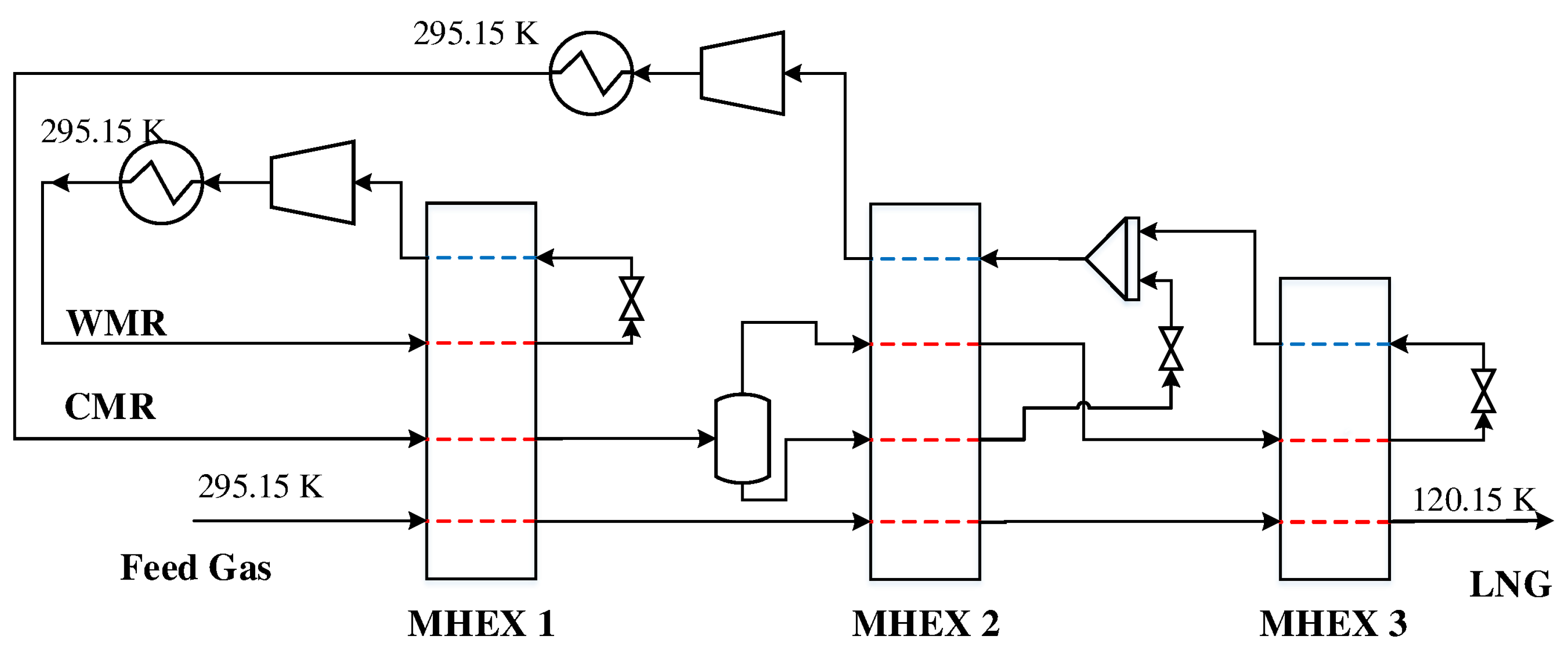
The first DMR process studied in this paper is a simple configuration with cascading PRICO cycles for the warm and cold mixed refrigerants. This cycle consists of two MHEXs as well as an NGL separator for the extraction of heavier hydrocarbons. Heavier hydrocarbons freeze out at cryogenic temperatures and can cause plugging in process equipment. Furthermore, they represent a valuable commodity if sold separately. The feed gas is sent to the process at 295.15 K where it is precooled by a warm mixed refrigerant cycle consisting of ethane, propane, and n-butane. The feed gas and the refrigerants exit the heat exchanger at a temperature of . The feed gas is then sent to the NGL separator, where heavier hydrocarbons are extracted for further fractionation and/or export, before the gas enters MHEX 2 for liquefaction. The cold mixed refrigerant consists of a lighter refrigerant mixture consisting of nitrogen, methane, ethane, and propane for the liquefaction of the natural gas. Along with the feed gas, the CMR is precooled in the WMR PRICO cycle before it enters the cold heat exchanger. A process flowsheet of the DMR process is presented in Figure 1.
The parameter values and initial guess values for the unknown variables are provided in Table 1. The parameter values were selected such that Aspen Plus failed to converge to a feasible solution using its standard MHEX model with one equation. Essentially, the Aspen Plus model only solves the overall energy balance in Equation (4) for a single unknown temperature (chosen here as the inlet inlet temperatures to the compressors). Refrigerant compositions and pressures cannot be handled as unknown variables in these models. This results in less versatility in cases where pressure, compositions, and multiple temperatures must be adjusted to find a feasible design.
The model contains 61 unknowns, five of which are provided by the solution of the MHEX equations. The remaining 56 variables are the temperatures of the intermediate stream segments for the single phase regions. As flash calculations are decoupled and solved separately, the model size is independent of the number of stream segments in the two-phase region. A two-equation model is used for MHEX 1 as the -value depends on the stream results from MHEX 2. Fixing the area prior to simulation can therefore be challenging. Therefore, the heat exchanger conductance value is instead calculated through post-processing. The simulations were carried out for a rich feed gas composition with 1.00 mol % nitrogen, 85.60 mol % methane, 4.93 mol % ethane, 3.71 mol % propane, 2.90 mol % n-butane, 1.30 mol % i-butane, and 0.56 mol % n-pentane at a pressure of 4 MPa and flowrate of 1.0 kmol/s where both the refrigerant mixtures and the feed gas enter the precooling MHEX at a temperature of 295.15 K, as indicated in Figure 1. Two simulation cases were constructed, solving for different sets of unknown variables:
- Case I:, , , , .
- Case II:, , , , .
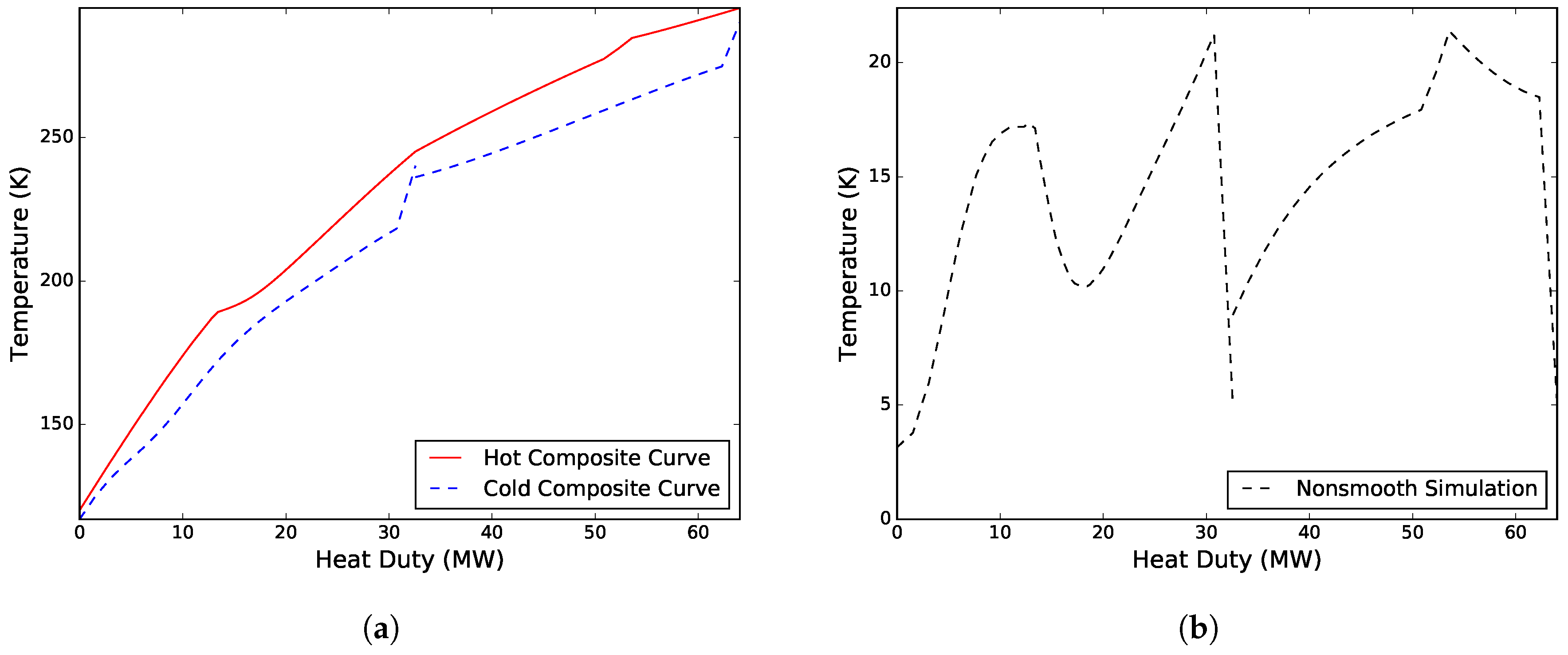
Case I. Solved for a variable WMR composition, an unknown inlet temperature to the CMR compressor, the heat exchanger conductance in MHEX 2, as well as the low pressure level and high pressure level of the warm and cold mixed refrigerants, respectively. The refrigerant composition was changed in the model by varying the component molar flowrate of propane . A solution was obtained after four iterations and a total simulation time of 62.7 s, including initialization. The model converged to a solution with MPa, MPa and K. The design resulted in a total compression work of 21.33 MW, with heat exchanger conductance values of MW/K and MW/K. The work distribution of the two compressors was 16.79 MW for compressing the CMR and 4.54 MW for compressing the WMR. A new WMR composition was obtained consisting of 53.30 mol % ethane, 26.64 mol % propane and 20.06 mol % n-butane with a corresponding molar flowrate of 1.48 kmol/s. Figure 2 presents the composite curves and driving force plot for the solution.
Case II. Solved for the flowrate of the CMR, the minimum approach temperatures in both MHEXs, and the high pressure and low pressure levels of the warm and cold refrigerant mixtures, respectively. A solution was obtained after 13 iterations with MPa, MPa, kmol/s, and minimum approach temperatures of 5.00 K and 3.15 K for MHEX 1 and 2, respectively. The design resulted in a total compressor work of 20.56 MW, and a heat exchanger conductance value of 2.04 MW/K. Compressing the CMR required a total of 14.10 MW, whereas compressing the WMR required only 6.46 MW. The total simulation time, including initialization of the model, was 102.5 s. The composite curves and driving force plots for the process are presented in Figure 3. As can be seen, both solutions have a similar trend, although the cold low pressure refrigerant superheating is noticeably larger in Case I. This results in lower driving forces in MHEX 1, but also introduces a larger temperature difference at the cold end of the process, leading to a higher compression power. A discussion on superheating and its effect on design of DMR processes was made by Kim and Gundersen [29].
5. Example 2
A more complex DMR design is presented in Figure 4. Instead of having two cascading PRICO cycles, this design features a spiral-wound heat exchanger (SWHX) for the CMR where the refrigerant is separated after precooling to provide cooling at different temperature levels. The vapor product, which consists mainly of the light components nitrogen and methane, is liquefied and subcooled to provide cooling in the cold MHEX 3. At the same time, the liquid product is subcooled and mixed with the low pressure refrigerant from MHEX 3, where it is used to cool the feed gas in the intermediate MHEX 2. Since part of the refrigerant mixture only circulates in the warm end of the SWHX, the overall molar flowrate and thus the required heat transfer area decrease.
The refrigerant streams and MHEX data for the DMR model are given in Table 2. Again, the parameter values were selected such that a solution could not be obtained using the commercial simulation tool Aspen Plus. A feed gas composition with 1.00 mol % nitrogen, 91.60 mol % methane, 4.93 mol % ethane, 1.71 mol % propane, 0.35 mol % n-butane, 0.40 mol % i-butane, and 0.01 mol % i-pentane at a pressure of 5.5 MPa and a flowrate of 1.0 kmol/s was used in the simulations.
The simulation model with three MHEXs consists of 96 variables and exhibits seven unknowns. Again these unknowns may be used to solve for any process stream variable such as the pressure, composition, flowrate, or temperature, as well as important MHEX data such as the minimum temperature difference and the heat exchanger conductance. Specifying the -value in MHEXs 1 and 2 is challenging as it depends on the solution of MHEX 3. Therefore, as for Example 1, the -values are calculated during post-processing to make problem specification easier. Two simulation cases were constructed solving for the following sets of unknown variables:
- Case I:, , , , , , .
- Case II:, , , , , , .
Case I: Solved for both pressure levels of the WMR, the low pressure level and refrigerant flowrate of the CMR, the feed gas and high pressure refrigerant temperatures out of MHEX 2, the low pressure refrigerant temperature out of MHEX 3, as well as the minimum approach temperature in MHEX 2. A solution was obtained after six iterations and a total simulation time of 83.0 s with MPa, MPa, MPa, K, K, kmol/s, and K. The -values were calculated to be 1.99 MW/K and 2.12 MW/K for MHEXs 1 and 2, respectively. The obtained feasible design resulted in a combined compression work of 14.40 MW, where 9.76 MW was needed to compress the CMR, and 4.64 MW was used to compress the WMR. Figure 5 presents the composite curves and driving force distribution in the MHEXs at the solution.
Case II: Solved for the low pressure level of the WMR, high pressure level of the CMR, the natural gas and high pressure refrigerant temperatures out of MHEX 2, the low pressure refrigerant temperature out of MHEX 3, the composition of the WMR, the minimum temperature difference in MHEX 2, and the heat exchanger conductance value for MHEX 3. The model converged after three iterations and a total simulation time of 64.2 s to a solution with MPa, MPa, K, K, K, and MW/K. A new WMR composition was obtained with 49.24 mol % ethane, 33.24 mol % propane, and 17.51 mol % n-butane and a total molar flowrate of 1.59 kmol/s. The feasible design required a total compression power of 14.85 MW, where 10.08 MW was spent compressing the CMR and 4.76 MW was used to compress the WMR. The heat exchanger conductance values were calculated during post-processing to be MW/K and MW/K, respectively. The composite curves and driving force plots for the process are presented in Figure 6.
Case III: Included an NGL separator for the extraction of heavier hydrocarbons (see Figure 7). The case solved for the same set of variables as in Case I and with the same initial guesses and parameter values as given in Table 2. As for the previous examples, the model was solved from an initial guess at which Aspen Plus obtained no feasible solutions with the built-in MHEX module. Rich feed gas compositions at a reduced pressure of 4.0 MPa were used to ensure adequate separation. Simulations were carried out at three different compositions with varying methane contents (Table 3).
Driving force distributions for the three solutions are provided in Figure 8. Solutions were obtained for all three cases within a few iterations. The first two feed gas compositions converged after seven iterations and total simulation times of 85.6 s and 86.4 s for compositions I and II, respectively. The third case converged after six iterations and a total simulation time of 82.1 s. All three solutions exhibited similar driving force profiles, with temperature differences varying mainly in the intermediate MHEX. The same trend can also be seen from the simulation results in Table 4, where the main differences between the three solutions are the and values for the intermediate MHEX.
6. Conclusions
This paper successfully simulated two different dual mixed refrigerant processes using recent modeling advances in the field of nonsmooth analysis. Natural gas liquefaction processes are particularly difficult to simulate with conventional process simulators, such as Aspen Plus. Lacking rigorous checks for preventing temperature crossovers means that the user must often resort to an iterative approach to obtain feasible designs. A multistream heat exchanger model that features rigorous checks for preventing temperature crossovers during simulation was included in the models. It includes nonsmooth formulations for pinch point location and phase regime detection in the heat exchangers. As a result, it offers a compact formulation where the flowsheet models can be simulated by solving a set of nonsmooth equations, rather than solving a local or global optimization problem. All the cases successfully converged within a total simulation time of 100 s, including initialization of the models. Furthermore, each case was constructed such that Aspen Plus failed to obtain a feasible solution using the same starting point and initial guess values as the nonsmooth model. The use of additional unknowns and the possibility of varying ostensibly difficult process stream variables, such as compositions makes the tool more versatile and capable of handling even complex LNG liquefaction processes.
Author Contributions
All of the authors contributed to publishing this paper. M.V. and H.A.J.W. developed the simulation models for performing the analysis; T.G. and P.I.B. provided useful mathematical and thermodynamical insight for developing the simulation tool and analyzing the results; M.V. wrote the paper; M.V., T.G., and P.I.B. revised and polished the manuscript.
Funding
HighEFF, Statoil.
Acknowledgments
This publication was funded by HighEFF—Centre for an Energy Efficient and Competitive Industry for the Future. The authors gratefully acknowledge the financial support from the Research Council of Norway and user partners of HighEFF, an 8 year Research Centre under the FME scheme (Centre for Environment-friendly Energy Research, 257632/E20). Harry A. J. Watson acknowledges Statoil for providing funding for this project.
Conflicts of Interest
The authors declare no conflict of interest.
Nomenclature
The following abbreviations are used in this manuscript:
| Roman letters | ||
| = | enthalpies of the extended composite curves (W) | |
| f | = | component molar flowrate (mol/s) |
| F | = | total molar flowrate (mol/s) |
| = | element of the generalized derivative | |
| = | heat capacity flowrate (W/K) | |
| = | total number of components | |
| T | = | temperature (K) |
| = | heat exchanger conductance (W/K) | |
| P | = | absolute pressure (Pa) |
| Q | = | heat duty (W) |
| = | equation residuals | |
| W | = | compressor work (MW) |
| Greek letters | ||
| = | log mean temperature difference (K) | |
| = | minimum approach temperature (K) | |
| = | enthalpy change (W) | |
| = | variable in the LP-Newton method | |
| Subscripts and superscripts | ||
| 2p | = | two-phase substream |
| BP | = | bubble point |
| C | = | cold stream |
| DP | = | dew point |
| in/out | = | inlet/outlet temperature of a substream |
| IN/OUT | = | inlet/outlet temperature of a process stream |
| H | = | hot stream |
| HP | = | high pressure refrigerant |
| LP | = | low pressure refrigerant |
| p | = | pinch candidate |
| sub | = | subcooled substream |
| sup | = | superheated substream |
References
- Hwang, J.H.; Ku, N.K.; Roh, M.I.; Lee, K.Y. Optimal Design of Liquefaction Cycles of Liquefied Natural Gas Floating, Production, Storage, and Offloading Unit Considering Optimal Synthesis. Ind. Eng. Chem. Res. 2013, 52, 5341–5356. [Google Scholar] [CrossRef]
- Aspen Technology Inc. Aspen Plus v9; Aspen Technology Inc.: Bedford, MA, USA, 2016. [Google Scholar]
- Aspen Technology Inc. Aspen HYSYS v9; Aspen Technology Inc.: Bedford, MA, USA, 2016. [Google Scholar]
- Kamath, R.S.; Biegler, L.T.; Grossmann, I.E. Modeling multistream heat exchangers with and without phase changes for simultaneous optimization and heat integration. AIChE J. 2012, 58, 190–204. [Google Scholar] [CrossRef]
- Watson, H.A.J.; Khan, K.A.; Barton, P.I. Multistream heat exchanger modeling and design. AIChE J. 2015, 61, 3390–3403. [Google Scholar] [CrossRef]
- Hasan, M.M.F.; Karimi, I.A.; Alfadala, H.; Grootjans, H. Modeling and simulation of main cryogenic heat exchanger in a base-load liquefied natural gas plant. Comput. Aided Chem. Eng. 2007, 24, 219–224. [Google Scholar] [CrossRef]
- Hasan, M.M.F.; Karimi, I.A.; Alfadala, H.; Grootjans, H. Operational modeling of multistream heat exchangers with phase changes. AIChE J. 2009, 55, 150–171. [Google Scholar] [CrossRef]
- Rao, H.N.; Karimi, I.A. A superstructure-based model for multistream heat exchanger design within flow sheet optimization. AIChE J. 2017, 63, 3764–3777. [Google Scholar] [CrossRef]
- Pattison, R.C.; Baldea, M. Multistream heat exchangers: Equation-oriented modeling and flowsheet optimization. AIChE J. 2015, 61, 1856–1866. [Google Scholar] [CrossRef]
- Austbø, B.; Løvseth, S.W.; Gundersen, T. Annotated bibliography—Use of optimization in LNG process design and operation. Comput. Chem. Eng. 2014, 71, 391–414. [Google Scholar] [CrossRef]
- Watson, H.A.J.; Vikse, M.; Gundersen, T.; Barton, P.I. Optimization of single mixed-refrigerant natural gas liquefaction processes described by nondifferentiable models. Energy 2018, 150, 860–876. [Google Scholar] [CrossRef]
- Watson, H.A.J.; Barton, P.I. Modeling phase changes in multistream heat exchangers. Int. J. Heat Mass Transf. 2017, 105, 207–219. [Google Scholar] [CrossRef]
- Khan, K.A.; Barton, P.I. A vector forward mode of automatic differentiation for generalized derivative evaluation. Optim. Methods Softw. 2015, 30, 1185–1212. [Google Scholar] [CrossRef]
- Duran, M.A.; Grossmann, I.E. Simultaneous optimization and heat integration of chemical processes. AIChE J. 1986, 32, 123–138. [Google Scholar] [CrossRef] [Green Version]
- Watson, H.A.J.; Vikse, M.; Gundersen, T.; Barton, P.I. Reliable Flash Calculations: Part 2. Process flowsheeting with nonsmooth models and generalized derivatives. Ind. Eng. Chem. Res. 2017, 56, 14848–14864. [Google Scholar] [CrossRef]
- Vikse, M.; Watson, H.A.J.; Gundersen, T.; Barton, P.I. Versatile Simulation Method for Complex Single Mixed Refrigerant Natural Gas Liquefaction Processes. Ind. Eng. Chem. Res. 2018, 57, 5881–5894. [Google Scholar] [CrossRef]
- Roberts, M.J.; Agrawal, R. Dual Mixed Refrigerant Cycle for Gas Liquefaction. U.S. Patent No. 6,269,655 B1, 8 July 2001. [Google Scholar]
- Maher, J.B.; Sudduth, J.W. Method and Apparatus for Liquefying Gases. U.S. Patent No. 3,914,949, 28 October 1975. [Google Scholar]
- Boston, J.F.; Britt, H.I. A radically different formulation and solution of the single-stage flash problem. Comput. Chem. Eng. 1978, 2, 109–122. [Google Scholar] [CrossRef]
- Watson, H.A.J.; Vikse, M.; Gundersen, T.; Barton, P.I. Reliable Flash Calculations: Part 1. Nonsmooth Inside-Out Algorithms. Ind. Eng. Chem. Res. 2017, 56, 960–973. [Google Scholar] [CrossRef]
- Watson, H.A.J.; Barton, P.I. Reliable Flash Calculations: Part 3. A nonsmooth approach to density extrapolation and pseudoproperty evaluation. Ind. Eng. Chem. Res. 2017, 56, 14832–14847. [Google Scholar] [CrossRef]
- Grossmann, I.E.; Yeomans, H.; Kravanja, Z. A rigorous disjunctive optimization model for simultaneous flowsheet optimization and heat integration. Comput. Chem. Eng. 1998, 22, 157–164. [Google Scholar] [CrossRef]
- Clarke, F.H. Optimization and Nonsmooth Analysis; SIAM: Philadelphia, PA, USA, 1990. [Google Scholar]
- Nesterov, Y. Lexicographic differentiation of nonsmooth functions. Math. Program. 2005, 104, 669–700. [Google Scholar] [CrossRef]
- Khan, K.A.; Barton, P.I. Generalized Derivatives for Solutions of Parametric Ordinary Differential Equations with Non-differentiable Right-Hand Sides. J. Optim. Theory Appl. 2014, 163, 355–386. [Google Scholar] [CrossRef]
- Barton, P.I.; Khan, K.A.; Stechlinski, P.; Watson, H.A.J. Computationally relevant generalized derivatives: Theory, evaluation and applications. Optim. Methods Softw. 2018, 33, 1030–1072. [Google Scholar] [CrossRef]
- Facchinei, F.; Fischer, A.; Herrich, M. An LP-Newton method: Nonsmooth equations, KKT systems, and nonisolated solutions. Math. Program. 2014, 146, 1–36. [Google Scholar] [CrossRef]
- Fischer, A.; Herrich, M.; Izmailov, A.F.; Solodov, M.V. A Globally Convergent LP-Newton Method. SIAM J. Optim. 2016, 26, 2012–2033. [Google Scholar] [CrossRef]
- Kim, D.; Gundersen, T. Constraint formulations for optimisation of dual mixed refrigerant LNG processes. Chem. Eng. Trans. 2017, 61, 643–648. [Google Scholar] [CrossRef]
Figure 1.
The Dual Mixed Refrigerant (DMR) model with cascading PRICO cycles for the warm and cold mixed refrigerant streams.
Figure 1.
The Dual Mixed Refrigerant (DMR) model with cascading PRICO cycles for the warm and cold mixed refrigerant streams.

Figure 2.
(a) Composite curves for the feasible design in Case I. (b) The corresponding driving force plot.
Figure 2.
(a) Composite curves for the feasible design in Case I. (b) The corresponding driving force plot.

Figure 3.
(a) Composite curves for the feasible design in Case II. (b) The corresponding driving force plot.
Figure 3.
(a) Composite curves for the feasible design in Case II. (b) The corresponding driving force plot.

Figure 4.
The DMR process with a spiral-wound heat exchanger (SWHX) for the cold mixed refrigerant.

Figure 5.
(a) Composite curves for the feasible design in Case I. (b) The corresponding driving force plot.
Figure 5.
(a) Composite curves for the feasible design in Case I. (b) The corresponding driving force plot.

Figure 6.
(a) Composite curves for the feasible design in Case II. (b) The corresponding driving force plot.
Figure 6.
(a) Composite curves for the feasible design in Case II. (b) The corresponding driving force plot.

Figure 7.
The DMR process in Example 2 with natural gas liquid (NGL) extraction.

Figure 8.
Driving force distributions for the DMR process with NGL extraction.


Table 1.
Multistream heat exchanger (MHEX) and refrigerant stream data for Example 1. For unknown variables, the value listed is an initial guess.
Table 1.
Multistream heat exchanger (MHEX) and refrigerant stream data for Example 1. For unknown variables, the value listed is an initial guess.
| Property | Value | Property | Value |
|---|---|---|---|
| 0.8 | (MW/K) | 3.0 | |
| (K) | 3.0 | (K) | 3.0 |
| (kmol/s) | 1.65 | (kmol/s) | 1.55 |
| (MPa) | 1.67 | (MPa) | 4.30 |
| (MPa) | 0.42 | (MPa) | 0.25 |
| (K) | 245.15 | (K) | 120.15 |
| (K) | 290.15 | (K) | 240.15 |
| Composition (mol %): | |||
| Ethane | 47.83 | Nitrogen | 10.00 |
| Propane | 34.17 | Methane | 43.80 |
| n-Butane | 18.00 | Ethane | 35.20 |
| Propane | 11.00 |
Table 2.
MHEX and refrigerant stream data for Example 2. For unknown variables, the value listed is an initial guess.
Table 2.
MHEX and refrigerant stream data for Example 2. For unknown variables, the value listed is an initial guess.
| Property | Value | Property | Value |
|---|---|---|---|
| 1.0 | (K) | 4.0 | |
| (MW/K) | 0.3 | (K) | 11.0 |
| (K) | 4.0 | ||
| (kmol/s) | 1.55 | (kmol/s) | 1.45 |
| (MPa) | 1.67 | (MPa) | 4.85 |
| (MPa) | 0.50 | (MPa) | 0.25 |
| (K) | 240.15 | (K) | 170.15 |
| (K) | 120.15 | (K) | 280.15 |
| (K) | 230.15 | (K) | 145.15 |
| Composition (mol %): | |||
| Ethane | 47.83 | Nitrogen | 7.00 |
| Propane | 34.17 | Methane | 41.80 |
| n-Butane | 18.00 | Ethane | 33.20 |
| Propane | 18.00 |
Table 3.
Natural gas compositions for Case III.
| Compostion I: | Composition II: | Composition III: | |
|---|---|---|---|
| Nitrogen (mol %) | 2.00 | 2.00 | 2.00 |
| Methane (mol %) | 85.60 | 87.60 | 89.60 |
| Ethane (mol %) | 6.93 | 5.93 | 4.93 |
| Propane (mol %) | 3.71 | 2.71 | 1.71 |
| n-Butane (mol %) | 1.35 | 1.35 | 1.35 |
| i-Butane (mol %) | 0.40 | 0.40 | 0.40 |
| i-Pentane (mol %) | 0.01 | 0.01 | 0.01 |
Table 4.
Simulation results for the DMR process with NGL extraction.
| Composition I: | Composition II: | Composition III: | |
|---|---|---|---|
| Total work (MW) | 14.99 | 15.11 | 15.13 |
| (MW) | 10.26 | 10.40 | 10.43 |
| (MW) | 4.73 | 4.71 | 4.70 |
| (MW/K) | 2.07 | 2.05 | 2.03 |
| (MW/K) | 2.63 | 2.87 | 3.41 |
| (MPa) | 0.43 | 0.43 | 0.43 |
| (MPa) | 1.66 | 1.66 | 1.65 |
| (MPa) | 0.26 | 0.25 | 0.25 |
| (K) | 158.22 | 157.95 | 157.50 |
| (K) | 154.22 | 153.95 | 153.50 |
| (kmol/s) | 1.46 | 1.47 | 1.48 |
| (K) | 3.69 | 3.14 | 2.20 |
| LNG composition (mol %): | |||
| Nitrogen | 2.08 | 2.05 | 2.03 |
| Methane | 88.04 | 89.24 | 90.61 |
| Ethane | 6.50 | 5.68 | 4.81 |
| Propane | 2.67 | 2.15 | 1.48 |
| n-Butane | 0.52 | 0.65 | 0.81 |
| i-Butane | 0.19 | 0.23 | 0.27 |
| i-Pentane | 0.00 | 0.00 | 0.00 |
| LNG flowrate (kmol/s) | 0.96 | 0.97 | 0.98 |
© 2018 by the authors. Licensee MDPI, Basel, Switzerland. This article is an open access article distributed under the terms and conditions of the Creative Commons Attribution (CC BY) license (http://creativecommons.org/licenses/by/4.0/).
Share and Cite
MDPI and ACS Style
Vikse, M.; Watson, H.A.J.; Gundersen, T.; Barton, P.I. Simulation of Dual Mixed Refrigerant Natural Gas Liquefaction Processes Using a Nonsmooth Framework. Processes 2018, 6, 193. https://doi.org/10.3390/pr6100193
AMA Style
Vikse M, Watson HAJ, Gundersen T, Barton PI. Simulation of Dual Mixed Refrigerant Natural Gas Liquefaction Processes Using a Nonsmooth Framework. Processes. 2018; 6(10):193. https://doi.org/10.3390/pr6100193
Chicago/Turabian StyleVikse, Matias, Harry A. J. Watson, Truls Gundersen, and Paul I. Barton. 2018. "Simulation of Dual Mixed Refrigerant Natural Gas Liquefaction Processes Using a Nonsmooth Framework" Processes 6, no. 10: 193. https://doi.org/10.3390/pr6100193
Note that from the first issue of 2016, this journal uses article numbers instead of page numbers. See further details here.