Performance Assessment of a Boiler Combustion Process Control System Based on a Data-Driven Approach


School of Control and Computer Engineering, North China Electric Power University, Baoding 071003, China
*
Author to whom correspondence should be addressed.
Processes 2018, 6(10), 200; https://doi.org/10.3390/pr6100200
Submission received: 12 September 2018
/
Revised: 29 September 2018
/
Accepted: 16 October 2018
/
Published: 19 October 2018
(This article belongs to the Special Issue Design and Control of Sustainable Systems)
Abstract
:For the requirements of performance assessment of the thermal power plant control process, the combustion control system of a 330 MW generator unit in a power plant is studied. Firstly, the five variables that affect the process control performance are determined by the mechanism analysis method. Then, a data-driven performance assessment method based on the operational data collection from the supervisory information system was proposed. Using principal component analysis technique, we found that five different variables have different degrees of effect on the performance of the combustion process. By means of qualitative and quantitative analysis, five contribution rates of different variables affecting the performance index of the system were obtained. After that, the data is normalized to the non-dimensional variable, the performance assessment index of the boiler combustion process is defined, and the classification and assessment criterion of it are given. Through using the proposed method on the operation data of the 1# boiler and 2# boiler within 1 day, the performance indexes are calculated and achieved during different time periods. Analysis of the results shows that this method will not generate additional disturbance to the normal operation of the system, and it can achieve a simple, reliable, accurate and rapid qualitative and quantitative analysis of the performance of the boiler combustion control system, and also it can be extended and applied to other multivariable control systems.
1. Introduction
Modern thermal power plants generally have hundreds of control loops and thousands of control parameters, and the operating personnel find it difficult to monitor and improve all the controlled loop parameters and performance according to the traditional method, which leads to part of the control system possibly not working for a long time. If there is a lack of regular maintenance, the performance of the controlled system will decline as time goes on. The control performance of the power plant will reduce the effectiveness of the control system, which may reduce the output of electrical energy and increase the operation cost. Good performance of the control system is the safe and stable foundation of excellent operation of industrial processes, and also it is very significant to improve product quality, increase production efficiency, reduce the consumption of raw materials and energy consumption and prolong the service life of the equipment.
The important prerequisite to ensure the good operation of industrial processes such as thermal power plants is control system performance analysis, assessment and diagnosis, in order to analyze the operating condition of the control system, so as to provide suggestions to maintain the control system. Therefore, the problem of the control system performance analysis, assessment and monitoring has become increasingly prominent, and effective performance assessment and quantitative analysis of the control system has aroused more and more attention.
2. Development of Control Performance Assessment Method
Performance assessment of the control loop not only has great influence on the safety of industrial processes, but also plays a big role in improving the productivity, so the process engineers intensively hope to obtain a control performance assessment as an important indispensable reference. In 1989, Harris discussed and researched the closed-loop performance assessment in [1] for the first time, later named the “Harris index”, with the ratio of the process variable actual variance and the theoretical minimum variance as the performance index, quantitative analysis performance of the system. This article has attracted the attention of academics and engineers, prompting a number of research institutions and researchers to expand research on it. In the past more than 20 years, control performance assessment (CPA) and control performance monitoring (CPM) have become the most active areas of research and a series of achievements have been obtained.
Traditional CPA and CPM methods are based on evaluating the gap between the current performance and the expected control benchmark. Generally speaking, the control performance assessment benchmark can be divided into three categories, namely, theoretical optimal benchmark, user defined benchmark and historical benchmark. The theoretical optimal benchmark, especially the minimum variance control (MVC) benchmark [2,3] and linear quadratic Gaussian (LQG) benchmark [4,5], are dependent on a sufficiently accurate description of the physical mechanism of the process model, including the structure and parameters. An accurate disturbance model is also necessary, however, due to various constraints of the process and model mismatch factors [6], in most practical cases, the lower bound of the theoretical performance is difficult to obtain. In contrast, the user-defined benchmark avoids the ideal assumption of the controlled process, which depends on the user’s own subjective preference, and therefore, it becomes easier to implement in practice. As a pure data driven CPA/CPM solution, the historical benchmark is derived from the past operating data, which is considered to have desirable properties. This method does not require the user to establish a physical model for identification test, and can be applied to different type and scale control systems. Affected by the MVC benchmark, a statistical performance index based on covariance is defined in [7,8], which only uses historical data for a period of time. In [9], an improved method based on the covariance index is proposed. The benchmark based on error variance or covariance is probably the most widely used in CPA, and it is generally believed that it originated from the theoretical performance assessment established by the MVC benchmark. In recent years, in the field of control performance monitoring and diagnosis, the slow feature performance analysis [10,11,12] based on a data-driven approach has been proposed, and it has become a new method of control system performance diagnosis technology [13,14,15,16].
The statistical analysis [17] method is a kind of theory used for monitoring. Process performance monitoring and diagnosis which is based on multivariate statistical projection technology received extensive attention in academia and industry, which has become a hot direction in process control field and widely used in industrial production. The most commonly used methods are principal component regression (PCR), canonical correlation analysis (CCA), Fisher discriminant analysis (FDA) [18] and hidden Markov model (HMM), especially the principal component analysis method (PCA) [19,20,21,22], independent component analysis (ICA) and partial least squares (PLS). The research in [23,24,25,26,27] showed significant advantages of multivariate statistical methods in the ability to deal with a large number of highly correlated variables, and because of its simple form and less design work, compared with model-based technology, the multivariate statistical methods have been widely used in industrial production process monitoring.
Since the 1990s, a large number of high thermal power units were put into operation, which marked Europe taking the leading position in the world in coal-fired power plant technology. European governments have taken more and more stringent restrictions to the emissions of pollutants of the thermal power plant. Making the construction of a new high efficiency and environmentally protective thermal power unit has become one of the important choices of the European power industry. Germany, Britain, Holland, Belgium and other Western European countries have been building a large number of 800~1100 MW thermal power units, the successful experience of development of these efficient thermal power units is worthy of study and reference. As early as 1997, the performance assessment and monitoring technology has been applied to thermal power plants [28] and the methods mainly used are neural network [29] and data mining technology [30,31,32,33,34].
As the most important secondary energy, coal-fired power generation currently accounts for about 70~80% of power generation in China, so one of the main tasks for engineers and technical personnel is how to take effective measures to monitor and assess the performance of thermal control systems. At present, the performance assessment and monitoring methods of process control are mainly based on mathematical models and data-driven methods. In recent years, an important direction is the use of data-driven technology, which is a class of technology that does not need to know the precise mathematical model of the system. The control system performance assessment methods based on a data-driven approach are based on massive data in real-time industrial processes or offline collection, using a variety of data processing technologies and statistical modeling methods, to carry on the proper analysis of the data in a certain range, and thus the performance monitoring and assessment of control system is obtained. At a power plant of higher level automation, the supervisory information system (referred to SIS) at the plant level has been widely used, so the operational data is easy to store and access, providing abundant data resources for performance analysis and calculation.
Based on the above analysis, this paper intends to use the user-defined performance index to quantitatively evaluate the performance of a boiler combustion process control system. The main contents of this paper are as follows: in the second section, the development of various control performance assessment methods are introduced; in the third section, the boiler combustion control process, which can simply be regarded as three inputs and three outputs control object is illustrated; in the fourth section, the principal component analysis technology is introduced, including the main idea, the mathematical model of the principal component, the method and properties of PCA; in the fifth section, through the mechanism analysis method, the five main variables are determined based on the analysis of the influence of the performance of the boiler combustion control system. Using principal component analysis, the contribution rates of five different variables to the system performance index are obtained. On the basis of the above, the definition and classification of the performance index are given, and the steps of performance assessment using sample data are given. In the sixth section, the performance index of user-defined and classification benchmarks are given, the scheme of data acquisition for 1# and 2# boiler combustion control system of a power plant is determined, and then the performance of the data is evaluated according to the steps introduced in the fourth part. Meanwhile the assessment results and the five main factors affecting the boiler combustion performance are analyzed, and the main measures and suggestions to improve the performance are put forward. Furthermore, the Scientific Apparatus Makers Association (SAMA) charts of the three sub control systems of the boiler combustion control system are given in order to improve the performance. Finally, the seventh section is the summary of the full text.
3. Boiler Combustion Control Process
At present, the industrial boiler is still the main thermal power in China, and thermal power installed capacity and power generation as a proportion of overall capacity and generation reaches 75% and 82% respectively. The amount of coal consumption in thermal power plants makes up more than 50% of the national coal consumption, and coal combustion will inevitably bring about sulfur dioxide and carbon dioxide emissions, about 45% and 40% of the country’s emissions respectively. The environmental pollution caused by coal-fired industrial boilers is very serious, so severe haze in vast areas of China has an important relationship with the inefficiencies combustion of coal recent years. Therefore, thermal power enterprises are facing severe energy saving and emission reduction pressure in the development of low carbon economy. Figure 1 is a schematic diagram of the thermal power plant system.
The combustion system is an important part of the coal-fired boiler, the coal can produce heat by burning to generate high-temperature and -pressure steam, and provide the rotating machinery (turbine) with mechanical energy to drive the output electric power of the generator. The general combustion control system should include a complete set of equipment to make coal chemical energy into heat energy, such as fuel system (including ignition system, pulverizing system, etc.), combustion equipment (ignition equipment, pulverized coal burner), flue gas system and the thermal control system ensuring combustion process safe, economical and stable [35,36].
The basic task of the boiler combustion process is to make the boiler combustion provide heat to adapt to the boiler steam load demand, while also ensuring the safety and economy of the boiler [37,38]. The combustion process control system has three control variables (the fuel supply , the forced air and the induced air ) and three adjusted variables (the main steam pressure , the oxygen content in flue gas and the furnace pressure ), and the adjustment of the controlled variables have had obvious effects on each other. This is because there is a mutual influence between objects within the control variables and adjusted variables. One adjusted variable may be influenced by several control variables, and the relationship between the inputs and outputs of the combustion process is shown in Figure 2.
One of the characteristics of a large unit is a relatively large number of monitoring points, at present, a 300 MW unit plant of I/O often reaches 4000~5000 points, and a 600 MW unit of I/O usually reaches more than 7000 points. With the development of the electric power industry, the scale of power production is expanding, the number of control loops of a thermal power plant system is increasing, and it is not realistic to monitor the performance of all control loops by manual inspection. The parameter change is fast, the control object is large and the control objects are related to each other. So, the traditional ways of monitoring boiler, steam turbine and generator respectively have been unable to meet the requirements of the operation of large units, it is necessary to use a high degree of automation. A large number of facts have proved that a large thermal power unit is not possible to achieve safe and economic operations with a high degree of automation.
In most of the thermal power plants in China, due to variation of coal species, the quality of the coal is generally poor, coupled with equipment modification, variable load operation, thermal tests of long time interval and other reasons during the actual operation of the boiler, the phenomenon that the boiler combustion can not reach the optimal state exists, so the performance assessment and optimization of operation are urgently needed to improve the safety, economy and environmental protection of the unit plant in a certain range.
With the increase of unit capacity and the increase of parameters, the safety, stability and economic operation of the unit is continuously improved, the automation level of the thermal power plant is also continuously improved, from the traditional manual control to unit centralized control. It must be pointed out that, after all, the automation system can only work according to the laws of the people’s budget, but the unit operation process is complex and random. Therefore, the automation system generally does not need to know the higher order intervention, but in certain circumstances requires manual prompting or coordination. That is, highly automated thermal power units are not without human intervention, but the need for a higher level of intervention. This shows that the higher level of automation of the unit requires that operators also should have a high level of technological and cultural knowledge.
The data acquisition system (DAS) of the distributed control system (DCS) stores a lot of operation-related data, although these data have been partially used, but their hidden information has not been fully excavated, which has restricted the use of information. The main reason lies in the multivariable and strong coupling of the data information, too many variables will often increase the complexity of the problem, so people naturally want to select a small number of important variables that contain abundant information, in this case, the principal component analysis method for data reduction is put forward.
4. Principal Component Analysis Technique
When we study practical problems, it is often required to collect multiple variables. But so that there is a strong correlation among them, these variables have more redundant information. If we use them directly, not only will the model be more complex, but it will also cause large errors because of the existence of multiple linear factors. In order to make full use of the data, we usually want to replace the original older variables with fewer new variables. At the same time, we need to reflect the information of the original variables as much as possible, so that the problem can be simplified.
The introduction of the principal component analysis method first appeared in the field of multivariate statistical analysis [39,40,41,42]. Its core idea is to reduce the dimensions of a set of data and keep the change information of the original data set as far as possible. It carries the statistical analysis on the relationship and the changes between various parameters in the production process, and all the initial variables will be integrated into several comprehensive irrelevant variables as little as possible, and these variables include the original reflected information as more as possible, so that the problem can be simplified, which provides the possibility of transforming data resources into benefits.
4.1. The Basic Ideas of PCA
Principal component analysis is a method of using a mathematical dimension reduction; it finds out some variables to replace many variables, and the amount of information of these variables includes the original variables as much as possible, but not related to each other. This method of statistical analysis of multiple variables into a small number of mutually independent variables is called principal component analysis or principal variable analysis [43,44,45,46].
4.2. Mathematical Model of PCA
Assuming that random variables are involved in the actual problem, denoted by , and it’s covariance matrix is
It is a non-negative matrix of order. Assuming the new synthetic variables are obtained form by the linear transformation, that is
or
The coefficient is a constant vector. The Equation (3) requires meeting the following conditions [47]:
- (1)
- The coefficient vector is a unit vector, that is
- (2)
- and are not related to each other, that is
- (3)
- The variances of are decreasing, i.e.,
Then, is known as the first principal component, is known as the second principal component, and so on; there are main components. The main ingredient is also called principal components, and is called principal component factor here.
4.3. Method and Property of PCA
When the covariance matrix of the population is known, the principal component can be obtained according to the following theorem [48,49,50].
Theorem 1.
Assuming the characteristic values of the covariance matrixare, and the corresponding orthonormal unit eigenvectors are, then theth principal component of is:
where , and
Proof.
Let , then it is a orthogonal matrix, and
If is the first principal component of , in which . Let
where ,, and
Only when (standard unit vector) before the establishment of equal, then
Therefore, the first principal component of is
and also the variance reaches the maximum.
If is the second principal component of , in which , and
Let
Then , , and
thus
Only when (standard unit vector) before the establishment of equal, then
Therefore, the second principal component of is
and the variance reaches the maximum. □
Similarly, get the rest expression of the principal components, and the principal component of the variance is equal to the corresponding characteristic value.
Theorem 1 shows that calculating the principal component of is equivalent to finding all eigenvalues of the covariance matrix of and the corresponding orthogonal unit vector. According to the characteristic of orthonormal eigenvector, from large to small value, the linear combination of coefficient of respectively represent the first, the second, until the th principal component of , and the variance of the principal component is equal to the corresponding eigenvalue.
Corollary 1.
If the principal component vector, the matrix, then, and the covariance of is
then the total variance of principal component is
Proof.
From the Equation (7), obviously , and also by the Equation (8), there is
also because
therefore
□
The corollary shows that the principal component analysis can decompose the total variance of original variables into the sum of variance of the uncorrelated variables . Due to , therefore describes the information extracted from the th principal component accounts for the share of the total information. We call
the contribution rate of the th principal component, and the sum of former principal components contribution rate is called the cumulative contribution rate, which indicates the degree of the former principal component providing the total information. Usually is selected to make the cumulative contribution rate more than 80%.
4.4. Principal Component of Standardized Variables
In the process of solving practical problems, we often encounter different variables with different dimensions, sometimes leading to the degree of dispersion value of each variable being larger, so when calculating the covariance matrix, possible variance is mainly controlled by the variance of large data, maybe leading to unreasonable results. In order to eliminate the influence of dimension, the original data is usually standardized. Let
where , .
4.5. Principal Component Analysis of Sample Data
In practical problems, the general covariance matrix of population is generally unknown, and the data is just from the sample observation data with a capacity of . Suppose
is a simple random sample taken from the population with a total capacity of . Sample covariance matrix and sample correlation matrix are as follows:
where .
Respectively, and act as the estimates of the population and , and then the sample principal component analysis is done according to the overall principal component analysis method.
About the sample principal component, assuming the sample covariance matrix is , and its characteristic value is , the corresponding unit orthogonal eigenvector is , and the th sample principal component is
When the observations are turned into Equation (13), we get observation samples of the th sample principal component as follows
which is called the score of the th sample principal component. At this time
The contribution rate of the th sample principal component is
The sum of the contribution rate of the previous principal components is the cumulative contribution rate .
The same with the population principal component analysis, in order to eliminate the influence of dimension, we can use the method in Equation (10) to normalize the sample, that is, let
Because the covariance matrix of the standardized sample data is the sample correlation matrix of the original data, then the principal component analysis is enough only from the sample correlation coefficient matrix.
5. Definition, Classification and Procedures of Performance Assessment Index
5.1. Definition of Performance Assessment Index
There are many factors that affect the performance of the boiler combustion control process, and the thermal efficiency is one of the most important factors. While the thermal efficiency of the boiler is an important indicator reflecting the economic operation of the boiler, the main indicators that directly determine boiler thermal efficiency include the fuel gas temperature, the boiler oxygen content, the carbon content of fly ash and the air leakage rate of the air preheater; some other factors affect the thermal efficiency of the boiler all through the above four indicators. Therefore, it can be considered that there are five variables that affect the performance of the boiler combustion process. The relationship between the five variables is given in the follow equations, then according to the degree and polarity of each variable on the process performance index, the contribution rate of each variable to the performance index is given, and further define the performance assessment index of different boilers combustion control process.
The calculation of the boiler thermal efficiency usually uses the inverse balance method, by measuring the percentage of the heat loss of the boiler , , , and , and then calculating the boiler thermal efficiency according to the Equation (17).
where
In the Equation (18), —the percentage of heat loss of fuel gas, %;
- —the heat that the dry flue gas takes away, kJ/kg;
- —the heat contained in the steam in flue gas, kJ/kg;
- —the net calorific power of coal, kJ/kg.
In the Equation (19), —the chemical incomplete combustion heat loss percentage, %;
- —the actual dry flue gas volume per kilogram fuel, ;
- —the content percentage of carbon monoxide in dry flue gas, %;
- —the content percentage of methane in dry flue gas, %;
- —the content percentage of hydrogen in dry flue gas, %;
- —the content percentage of heavy carbon hydride in dry flue gas, %.
In the Equation (20), —the mechanical incomplete combustion loss percentage, %;
- —the quality percentage of base ash coal received, %;
- —the percentage of average carbon content and ash content in coal ash, %;
- —the heat loss rate of stone coal that the mill discharges, %.
In the Equation (21), —the heat loss percentage, %;
- —the heat loss percentage under rated evaporation, %;
- —the boiler rated evaporation boiler rating, ;
- —the actual evaporation measuring boiler efficiency, .
In the Equation (22), —the physical heat loss percentage of ash, %;
- —the quality percentage of total ash content in ash and slag, %;
- —the quality percentage of total ash content in fly ash, %;
- —the quality percentage of total ash content in settlement ash, %;
- —the furnace slag temperature, °C;
- —the furnace flue gas temperature, °C;
- —the settlement ash temperature, °C;
- —the datum temperature, °C;
- —the specific heat capacity of furnace slag, ;
- —the specific heat capacity of fly ash, ;
- —the specific heat capacity of settlement ash, ;
- —the combustible material quality percentage in ash and slag, %;
- —the combustible material quality percentage in fly ash, %;
- —the combustible material quality percentage in settlement ash, %.
Under normal circumstances, if the thermal efficiency of the coal-fired unit increases, then the performance of the boiler combustion control process becomes better, so the influence of the variable on the control performance index is positive.
In general, the flue gas temperature of a 300 MW coal-fired unit increases every 10 °C, then the power supply coal consumption is decreased by about 1.5, thus the performance of boiler combustion control process is declining, so the influence of the variable on the control performance index is negative.
In general, the boiler oxygen content of a 300 MW coal-fired unit increases every 1%, then the boiler efficiency decreases by 0.2% to 0.3%, and the coal consumption for power supply increases 0.6~0.9 ; thus the performance of boiler combustion control process gets worse, so the influence of the variable on the control performance index is negative.
In general, for every 1% increase in fly ash in the boiler combustible matter content of a 300 MW coal-fired unit, according to the different ash content and heat of coal into the furnace, the thermal efficiency of the boiler is reduced from 0.1% to 0.5%, thus the performance of the boiler combustion control process becomes worse, and so the influence of the variable on the performance index is negative.
According to the relevant experience, it is known that for every 1% increase in the air leakage rate of the air preheater, the coal consumption increases about 0.1 ; thus the performance of boiler combustion control process is declining, so the influence of the variable on the control performance index is negative. From the view of the order of magnitude, the air leakage rate of air preheater has little effect on the coal consumption.
According to the influence polarity and its contribution rate of five variables on the performance of boiler combustion control process, the results are shown in Table 1.
According to Equations (15) and (16), as well as Table 1, the performance assessment index (PAI) is defined as follows.
The definition of control performance index of 1# boiler combustion process:
where
The definition of control performance index of 2# boiler combustion process:
where
5.2. Classification of Performance Assessment Index
The classification standard of the performance assessment index of the boiler combustion control process is shown in Table 2.
5.3. Performance Assessment Procedures
The principal component analysis is carried out by the sample observation data, then the contribution rates of different variables to the control performance are calculated, and the steps of calculating the performance assessment index are as follows:
- (1)
- According to the analysis of the boiler combustion control system, the main variables affecting the performance of the system are determined as the main component of the system performance;
- (2)
- Data sampling is carried out on the relevant variables, and the sampling data are standardized;
- (3)
- The sample correlation coefficient matrix is calculated and the characteristic value of it found;
- (4)
- According to the principal component analysis and Equation (15), the respective contribution rates of the main components of are calculated;
- (5)
- According to the definition of performance assessment index, Equations (23) and (25), the performance assessment index of different boiler combustion control process are calculated;
- (6)
- According to the classification of PAI shown in Table 2, the performance indexes are classified, and analysis and research will be done in depth.
6. An Example of Performance Assessment of Combustion Control System
6.1. Performance Assessment and Analysis Program
6.1.1. Data Acquisition Scheme
Since the beginning of the twenty-first century, the electric power enterprise has attached great importance to the construction of electric power information. With the rapid development of internet and real-time database technology, many power companies are planning and establishing supervisory information systems (SISs) for thermal power plants or the management information system (MIS). A real-time database set of the system is the core, and the database is a massive database, providing a good data platform for long-term preservation for performance monitoring and diagnosis. Monitoring and diagnosis of the unit’s performance has also become the main content of information monitoring system of thermal power plants.
In recent years, new units put into operation generally set up online monitoring systems in accordance with the requirements of “DL 5000–2000 thermal power plant design specification”, at the same time in order to adapt to the demand of information management, the majority of old units have also added this system for many years. Therefore, it is suggested to make full use of the convenient conditions brought by the online monitoring system to collect and store data.
6.1.2. Performance Assessment Scheme
The correct performance assessment scheme is one of the important conditions to ensure the performance test results of the unit with high reliability and good repeatability.
In the past online performance monitoring systems, single measurement results of various measuring parameters or the average value of short time performance index calculation are tended to be used, but any single measurement value or short time average value has great randomness; the random performance measurement often requires enough times or sufficient amount of data to be eliminate, for the thermal power unit such a complex dynamic production process is even more so. Therefore, high real-time performance requirements will inevitably lead to the lack of sufficient data to eliminate the impact of random performance assessment, and this is not helpful for the performance analysis. In addition, the variation of performance is a slow process, and not a sudden process, therefore, it is not necessary to require the unit performance monitoring system with high real-time performance. Prevention and monitoring of some unexpected destructive accidents should not be included in the unit performance monitoring system, but should be included in the unit’s protection system.
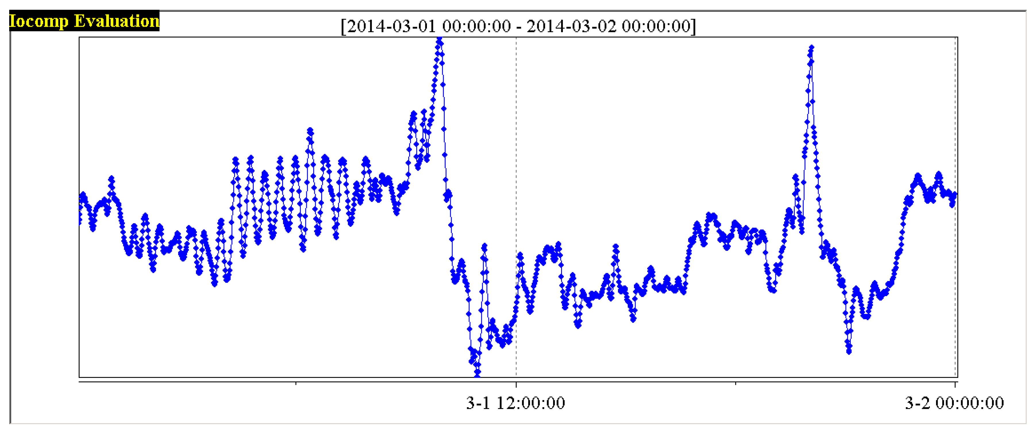
Because of the reasons above, the supervisory information system acts as the data acquisition platform, using the trend analysis software to resample the relevant data within 24 h for two boilers in a certain power plant in 1 March 2014, and the sampling period is 1 s.
6.2. Data Acquisition and Standardization of Two Boilers
Through the information monitoring system of a power plant, according to the five variables influencing the performance of the boiler combustion process shown in Table 1, the data of the five original variables of 1# boiler, that is, the boiler thermal efficiency , the flue gas temperature , the boiler oxygen content , the carbon content of fly ash , and the air leakage rate of air preheater are respectively shown in Figure 3, Figure 4, Figure 5, Figure 6 and Figure 7. In order to have a clearer analysis, the data of the five variables are put in one diagram, as shown in Figure 8.
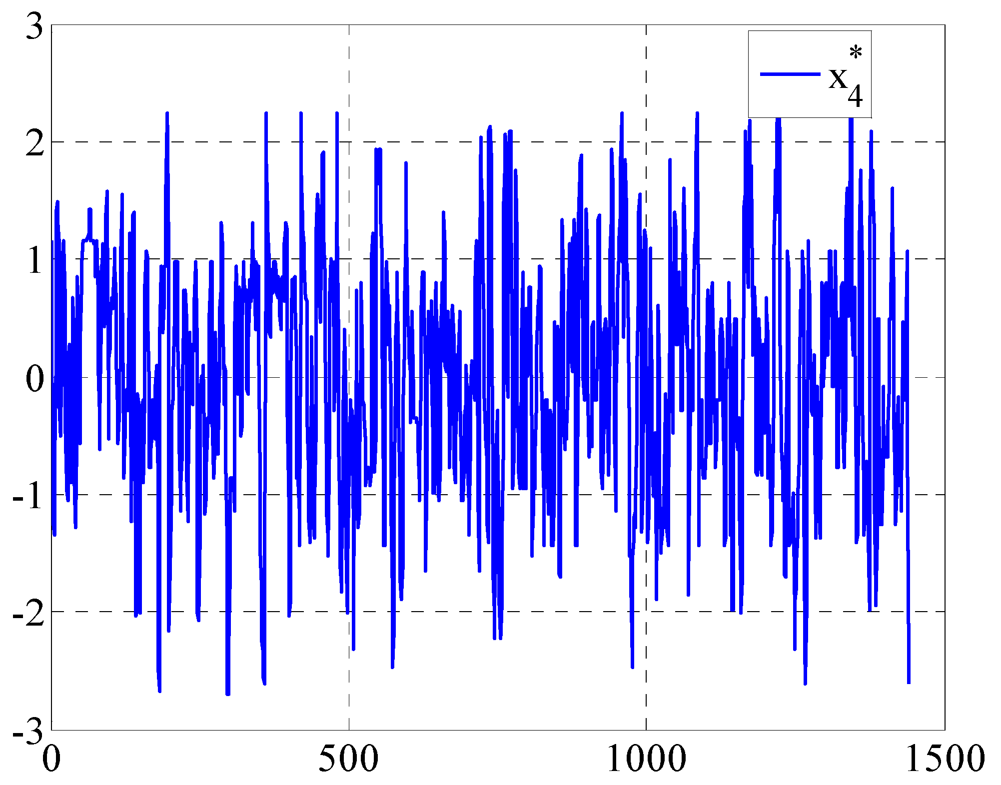
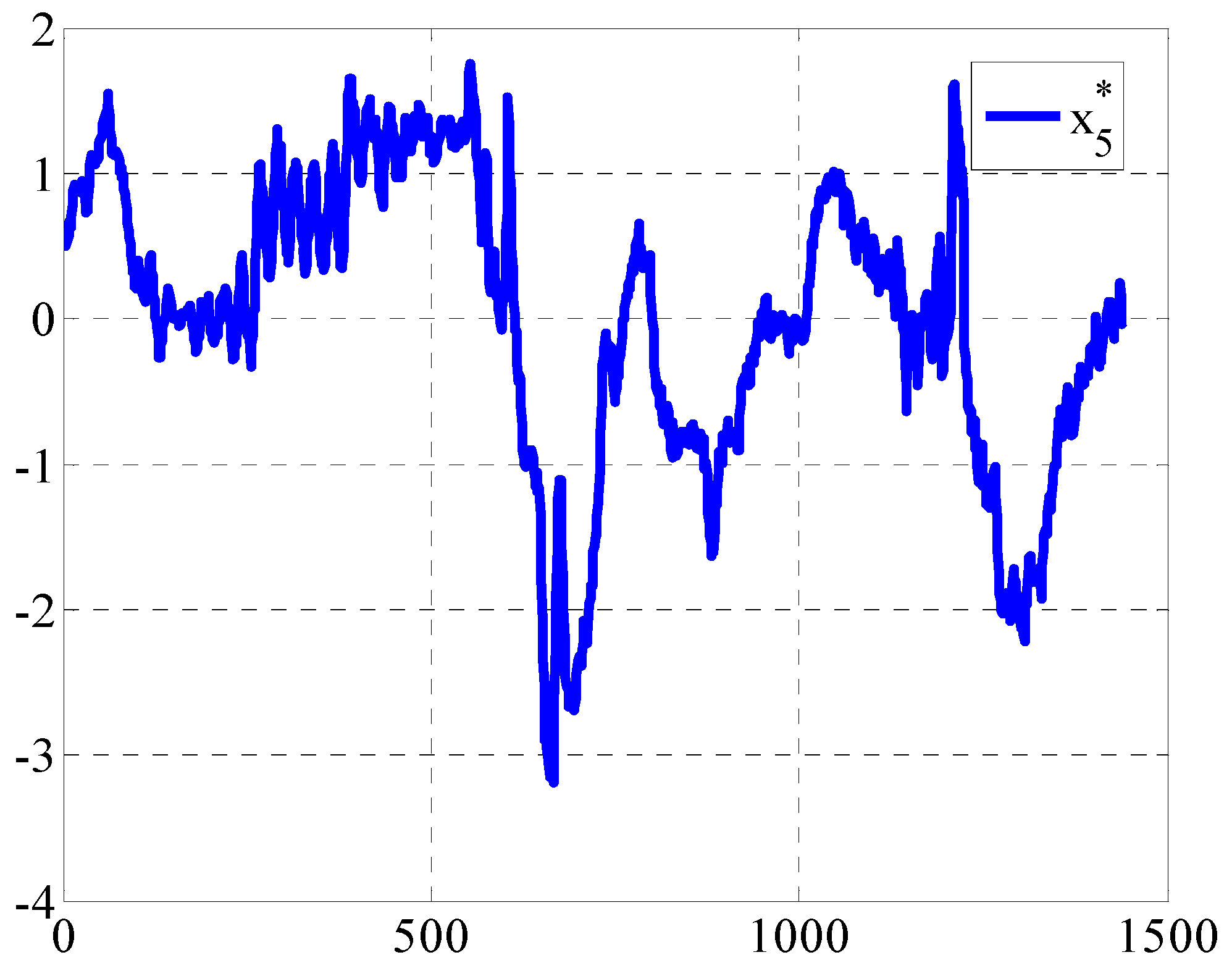
According to the Equation (16) in Section 4.5, the five variables of 1# boiler, , , , and , respectively gets the standardized treatment, gaining the standardization of the variables, , , , and , the results as shown in Figure 9, Figure 10, Figure 11, Figure 12, Figure 13 and Figure 14.
Similarly, the five original variables of the 2# boiler are as shown in Figure 15, Figure 16, Figure 17, Figure 18 and Figure 19 respectively. In order to be more clear, the data of the five variables are put in one diagram, as shown in Figure 20.
Similarly, according to the Equation (16) in Section 4.5, the five variables of 2# boiler, , , , and , respectively gets the standardized treatment, gaining the standardization of the variables, , , , and , the results as shown in Figure 21, Figure 22, Figure 23, Figure 24, Figure 25 and Figure 26.
According to the Section 4.5 and the sample data above, utilizing the Equation (16), in one day, the standard average data of different time periods are calculated, as shown in Table 3.
6.3. Performance Assessment Results
At the same time, according to the performance assessment procedures given in Section 5.3, the sample observation data given in Section 6.2 were analyzed by principal component analysis, then the contribution rates of five variables on the performance of boiler combustion control process were gained, and the results are shown in Table 4.
The coefficients in Table 4 were substituted into the Equations (23) and (25) respectively, then the formula of the performance assessment index of the combustion process of two boilers are obtained.
Definition of (Performance Assessment Index 1) for the 1# boiler combustion control process:
Definition of (Performance Assessment Index 2) for the 2# boiler combustion control process:
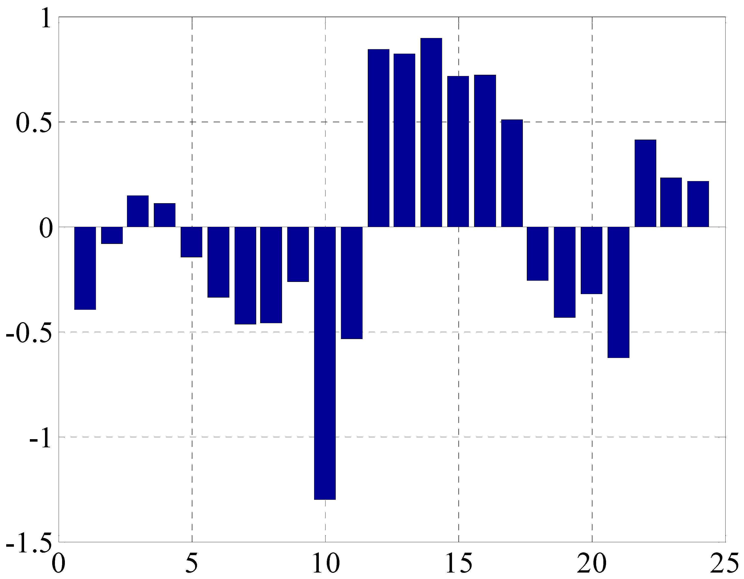
The data in Table 3 were substituted into the Equations (27) and (28) respectively, then the PAI values of 1# and 2# boiler combustion process corresponding to the different time periods in one day are obtained, and the results and PAI ranking are shown in Table 5.
From the Table 4, the performance of the 1# boiler and 2# boiler are shown respectively in Figure 27 and Figure 28 during 1 March 2014.
According to the classification criteria of the performance index in Table 2, the performance indexes of 1# boiler combustion control system are arranged according to the sequence from big to small, and the assessment results are classified, at the same time the percentage of different performance levels is calculated, and the statistical results are shown in Table 6.
According to the data in Table 6, the performance indexes of the 1# boiler are sorted, as shown in Figure 29.
Similarly, according to the classification criteria of the performance index in Table 2, the performance indexes of the 2# boiler combustion control system are arranged according to the sequence from big to small, and the assessment results are classified, at the same time the percentage of different performance levels is calculated, and the statistical results are shown in Table 7.
6.4. Analysis of the Results of Performance Assessment in Depth
According to the performance assessment results obtained in Section 6.3, further analysis is made on the various variables that affect the combustion performance of the boiler.
6.4.1. The Boiler Thermal Efficiency
Boiler thermal efficiency is a comprehensive index reflecting the economic operation of the boiler, and the degree of influence on the performance of the boiler combustion control process is also the largest. The main factors that directly determine the thermal efficiency include the fuel gas temperature, the boiler oxygen content, the carbon content of fly ash and the air leakage rate of the air preheater; some other factors affect the thermal efficiency of the boiler all through the above four variables. Therefore, in order to improve the performance of the boiler combustion control process, it is needed to find the countermeasures from the above four variables, and the details are as follows.
6.4.2. The Flue Gas Temperature
Flue gas temperature is the temperature of the flue gas from the last stage of the heating surface (this generally refers to the air preheater). In general, the design flue gas temperature of coal fired boiler is between 120 °C and 140 °C.
At present, domestic coal-fired power plant flue gas temperature is generally high in China; the main reasons for this, in terms of design, include that the heating surface layout is not reasonable, there is insufficient area of the heating surface of the coal saving device, the air preheater heat storage plate area is small, and so on. For example, the No.1 boiler in a power plant in Hainan, because of the small area of the air preheater and economizer, leads to a flue gas temperature that is higher than the design value by more than 20 °C, and so the boiler efficiency decreases by about 1%, and affects the power supply coal consumption 3.0 g/(kW·h). The main reason of operation is the fired coal greatly deviates from the design coal, especially where power plants burn a large amount of lignite. Due to the characteristics of low calorific value and high moisture of the coal, combustion conditions in the furnace change and the combustion flue gas volume increases, leading to increased gas temperature. The operation modes are not reasonable, including the primary air rate, operating mode of the coal grinding machine and operation units, coal mill outlet temperature control level, and so on; the combustion state of flame whitewashing, heating surface of dust coking, coal pulverizing system mixed with large amount of cold, poor tightness caused high air leakage rate; air preheater heat exchanger fouling, and so on.
The main measures to decrease the flue gas temperature are as follows:
- (a)
- Controlling the proper excess air coefficient in the furnace. By optimizing the combustion adjustment of the boiler, the oxygen content can be reduced and the heat loss of the boiler can be reduced under the condition that the pulverized coal is fully burned.
- (b)
- According to the change of load, adjust the burner operation mode, control center position of flame, reduce flame whitewashing, and avoid dust deposition.
- (c)
- When the coal quality changes, adjust the operation mode of coal pulverizing system in a timely fashion, guarantee the fineness of pulverized coal economy at the same time, and that the operating mode of the coal grinding machine, operation units and the outlet temperature of the coal mill are optimized.
- (d)
- To strengthen the operation and maintenance of the soot blower, to ensure the rate of the ash blowing equipment put into operation, to prevent the heating area of ash.
- (e)
- The economizer and the heated surface of the low temperature superheater or reheater are transformed by technology, reducing flue gas temperature.
6.4.3. The Boiler Oxygen Content
The oxygen content is the percentage of oxygen content in the flue gas of the furnace outlet, which reflects the excess air content in the combustion process, and affects the heat loss of the boiler. Operation oxygen is equal to the oxygen content of flue gas of boiler combustion control and the oxygen measuring point of air leakage. Therefore, in the process of thermal power unit operation, maintaining a reasonable amount of flue gas oxygen content can improve the operating economy and reliability of thermal power generation units.
Operation oxygen directly affects the boiler combustion conditions; in the case of other conditions unchanged, with the increase of oxygen content of the boiler the excess air coefficient increases, combustion oxygen supply is sufficient, air mixing disturbance increases, combustion efficiency of pulverized coal improves, and fly ash combustible content decreases, reducing the boiler mechanical incomplete combustion heat loss, but at the same time, boiler flue gas volume increases, the heat loss of exhaust gas increases, power consumption rate of the fans also increases, and concurrently overheating and reheat desuperheat water increase, and production increases. Therefore, considering the mechanical incomplete combustion heat loss, the exhaust heat loss, the wind turbine power consumption rate, the reduction of warm water and the amount of oxygen, the boiler oxygen generated to achieve the optimal becomes the best oxygen content.
The optimal oxygen content of the boiler is changed according to the load of the unit, the state of operation and the changing quality of the coal. At present, the domestic power plant coal-fired boiler oxygen content is usually controlled by operators according to the experience, which has great randomness, at the same time, there is a deviation between the operation of the dial and the actual amount of oxygen, and the actual amount of oxygen in the unit is deviated from the optimum oxygen content, which leads to the economic decline of the unit.
The determination of the optimal oxygen content of the boiler is usually after the boiler overhaul, the coal quality changed or the burner is reformed, boiler combustion adjustment test is carried out, while maintaining the primary air rate and coal pulverizer operation mode under the suitable conditions, the combustible matter in fly ash, the heat loss of exhaust gas, the fan power consumption rate, reheater desuperheating water and production are compared under different operation oxygen, so the optimal oxygen content corresponding to different load is determined, thus not only improving the running efficiency, but also improving the performance of the boiler combustion control.
6.4.4. The Carbon Content of Fly Ash
Combustible ash includes fly ash and slag combustible materials. For a pulverized coal fired boiler in a power plant, usually the ratio of the content of fly ash and slag ash is considered 9:1, therefore, the influence of fly ash on the economic performance of the unit is more significant than that of the slag, the combustible matter in fly ash is usually the focus of attention of the economic analysis of power plant.
Coal quality is the most important factor affecting the combustible ash. At present, for the boiler burning bituminous coal and lignite, the combustible ash is generally within 2%, and the corresponding mechanical incomplete combustion heat loss is usually lower than the design value. As for a boiler burning anthracite, lean coal, anthracite and lean coal blending, the combustible matter in fly ash usually reaches 2% to 3%, for some of the units up to more than 5%, which is the main reason of low efficiency of the boiler.
Pulverized coal fineness also has an important influence on the combustible ash. The relative fineness of pulverized coal helps to reduce the combustible ash, solid incomplete combustion heat loss is relatively low, but also increase the power consumption rate of coal powder system and wear, comprehensive considering the combustible ash and coal pulverizer power consumption rate, the optimal fineness is called optimal coal fineness.
According to different types of coal and flour milling systems, the best fineness of pulverized coal is different, which usually needs to be determined by the optimization and adjustment of the combustion system. According to the general rules, for burning bituminous and lignite coal boiler, combustible ash is relatively low, considering the coal pulverizer outlet fineness appropriate to be thick, usually coarse pulverized coal fineness can be put to around 30%, ensuring the combustion efficiency of combustible and ash are relatively low, helping to reduce the power consumption rate of the coal grinding machine, improving the mill output and unit economy. For burning anthracite, in a lean coal boiler, the combustible matter in fly ash is relatively high, in which the coal mill meets the unit output requirements, but at the same time should, as far as possible, ensure the coal pulverizer outlet fineness is smaller; usually, the fineness of pulverized coal can be maintained at around 15%, some hard to burn coal to keep within 10%, to help reduce the combustible ash, not only improving the economical efficiency of the unit, but also improving the performance of the boiler combustion control.
6.4.5. The Air Leakage Rate of Air Preheater
The ratio of the air quality leaking into the air preheater flue gas side and the quality of the flue gas entering the flue is called air leakage of air preheater. It is a comprehensive indicator to reflect the design, manufacturing and economy of the air preheater. Its impact on the economy of the boiler is mainly reflected in the impact on the power consumption of the blower and the air preheater heat transfer rate, the degree of influence is closely related to the occurrence of air leakage. Therefore, generally when the air preheater leakage rate is controlled between 6% and 7%, the unit economy is relatively good.
At present, the air preheater that coal-fired boilers are equipped with consists of the tube and rotary type in China, which take a long time to put into production. Small capacity boilers usually adopt the tube type air preheater, and its air leakage rate is larger, which is mainly related to the pipe leakage caused by wear, blockage, corrosion or installation (maintenance), and quality the control of the air pressure of the air supply fan during operation.
For large capacity and new units, a three sectional regenerative air preheater is widely used in power plants in China, and the rotary air preheater leakage rates are mainly related to preheater sealing structure, sealing seal clearance changes, automatic tracking system input, blowing equipment supply, maintenance quality and operation cycle.
The measures to reduce the air preheater leakage rate includes the maintenance period of strict adjustment of air preheater leakage during operation; regularly checking the seal automatic tracking device; timely adjustment; strengthening the maintenance; regular air preheater leakage testing; timely detection of air leakage of the air preheater; air preheater to prevent corrosion and fouling.
6.5. The Main Measures to Improve the Performance
Based on the analysis and discussion in Section 6.4, the main factors that influence the combustion performance of the boiler are analyzed, and the main measures and suggestions are given to improve the performance of the boiler combustion process below:
- (1)
- As far as possible to ensure the stability of the boiler burning coal quality and running load stability;
- (2)
- According to the factors of coal quality, unit load and combustion equipment, the optimization of combustion adjustment test is carried out in a timely manner;
- (3)
- Reasonable control of the excess air coefficient of the boiler or the air flow rate into the furnace;
- (4)
- Reasonable control of the fineness of pulverized coal;
- (5)
- Reduce the air leakage of the boiler, air preheater, smoke ventilation system and coal pulverizing system;
- (6)
- Reduce automatic coordinated control operation of the boiler and put the boiler air temperature and the air pressure into automatic control system in time;
- (7)
- The steam turbine and the boiler on-line optimization operation system uses the method of energy consumption analysis and so on, displaying the economic and technical parameters of the boiler, the actual value and the target value, guiding the personnel’s economic operation;
- (8)
- Implementation of a strict periodic purge system, to ensure the timely removal of ash fouling of heating surface, improve the efficiency of heat transfer, reduce gas temperature;
- (9)
- Strengthen the heat preservation, reduce the heat loss;
- (10)
- Controlling the quality of water and steam;
- (11)
- Prevent water and steam leakage.
6.6. An Example of Boiler Combustion Control System
In the application of the actual power plant, in order to show how to improve the performance of the boiler combustion control system, taking the combustion control system of intermediate storage type boiler as an example, three sub control systems, SAMA (Scientific Apparatus Makers Association) diagrams of fuel quantity control system, air volume control system and furnace pressure control system are respectively given as follows.
6.6.1. The Fuel Quantity Control System
The main fuel of a coal fired boiler is coal, because the fuel system is of an intermediate storage type, so by adjusting the speed of the coal supply machine to adjust the amount of fuel, the input signal of fuel quantity control is the main boiler directive and the output signal is the speed of coal supply machine instructions. In the boiler combustion process, if the air is too little, it will cause the fire of the furnace to be out, in order to ensure the complete combustion of the fuel, the air flow should always be richer than the fuel. The SAMA diagram of the fuel quantity control system is shown in Figure 31.
6.6.2. The Air Volume Control System
For the fuel into the furnace to be fully burned, which is directly related to the economy of boiler combustion, the air flow into the furnace should be controlled. The larger is selected between the heat signal (HR) and boiler main directive (BD), realizing the cross restriction of wind and coal, and to make the total amount of wind always been richer than fuel. When the load increases, that is, when the main instructions of the boiler increases, first add the wind, then add coal; when the load reduces, first reduce coal, then reduce wind. The SAMA diagram of the air volume control system is shown in Figure 32.
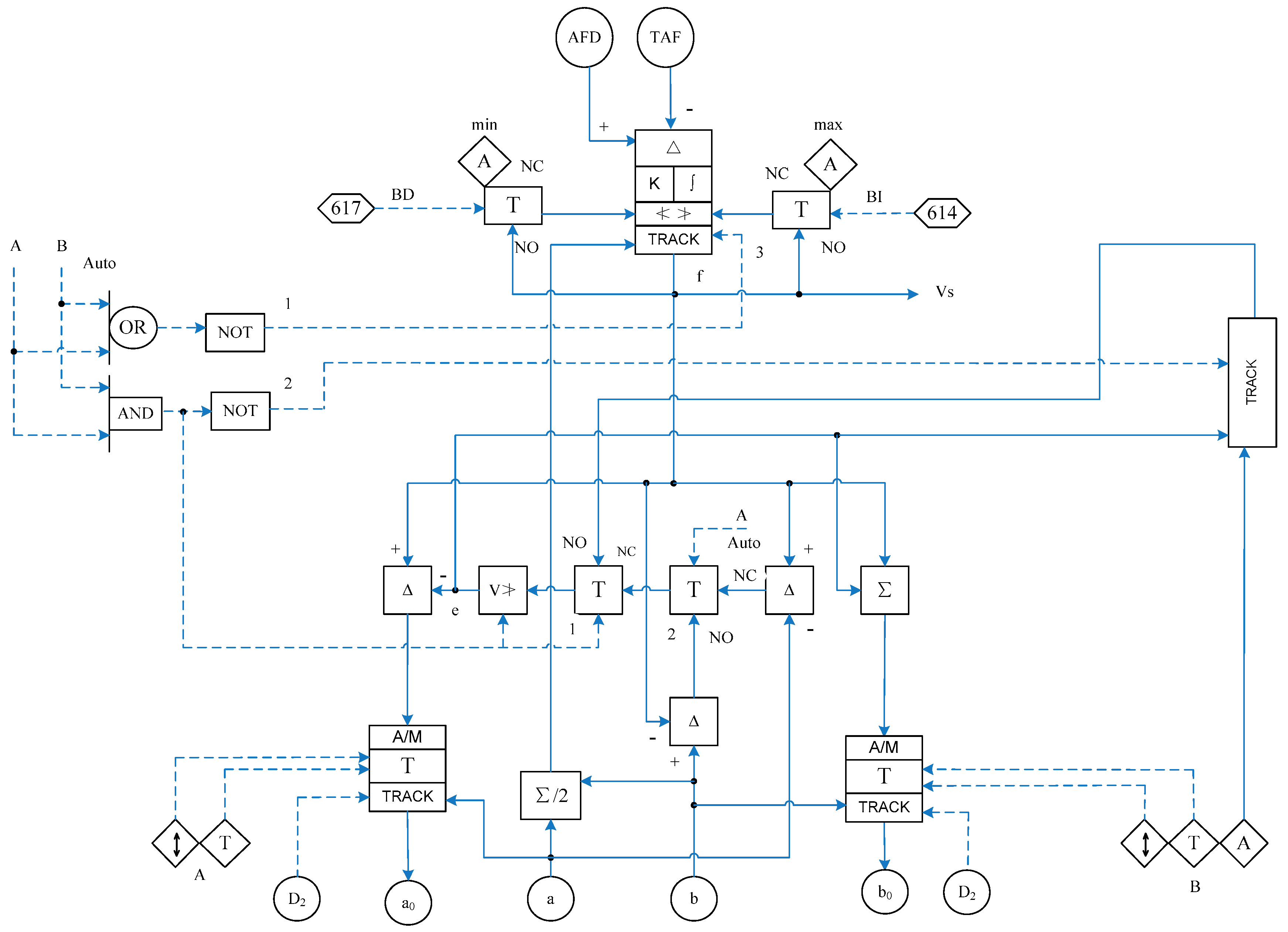
6.6.3. The Furnace Pressure Control System
The furnace pressure is related to the safety and economic operation of the boiler. High furnace pressure will result in the increase of the power consumption of the fan and the increase of the heat loss of the exhaust gas. Low furnace pressure will cause the danger of explosion. Therefore, it is necessary to control the furnace pressure in the safe and allowable range, the control method is based on the adjustment of the furnace pressure and the air flow rate of the boiler. The SAMA diagram of the furnace pressure is shown in Figure 33.
7. Conclusions
In the process of thermal power generation, the performance of the boiler combustion control system affects the thermal efficiency of the whole power plant, so reasonable and effective performance assessment can improve the economic performance of the whole power plant. The universal application of the distributed control system and supervisory information system in power enterprises provides the data for the control system performance assessment technology.
In this paper, based on the mechanism analysis method, the five main variables that affect the performance of the boiler combustion control system are put forward, and then, using principal component analysis method, respective contribution rates of five variables on the performance of the process control are obtained; meanwhile the performance assessment indexes for two boiler combustion control systems are defined.
Based on the acquisition data of 1# and 2# boilers, performance indexes of different time periods are calculated, and the results show that the performance index can reasonably and correctly evaluate the performance of the control system of boiler combustion. At the same time, the influence of each variable on the control performance of the boiler combustion process is analyzed, and the measures and suggestions to improve the performance of the system are given. Then, taking the combustion control system of intermediate storage type as an example, the SAMA control block diagram of the three sub control systems are presented.
Because the performance evaluation process does not need to establish a complex physical model, and the calculation is small, and also there is no interference to the closed-loop control system, it can be extended to other multivariable control systems. This method can be a substitute for manual inspection of the automatic performance monitoring, which can early monitor the control performance, thereby reduce the workload of the engineers and operation and the downtime in the production process of power generating units, increase the plant operation safety, and can reduce the production cost of electricity. These factors are of great significance and practical value for the safety and economical operation of a power plant.
Author Contributions
S.L.: figures, study design, data analysis, writing; Y.W.: literature search, data collection, data interpretation.
Funding
This work were supported by the Fundamental Research Funds for the Central Universities (No.2017MS189), and the Hebei province higher education teaching reform and practice project (No. 2016GJJG318).
Conflicts of Interest
The authors declare no conflict of interest.
References
- Harris, T.J. Assessment of control loop performance. Can. J. Chem. Eng. 1989, 67, 856–861. [Google Scholar] [CrossRef]
- Shin-ich, Y.; Tomohiro, H.; Akira, I.; Akira, Y.; Mingcong, D. Mathematical Expressions of Controller Poles and Steady Gain of Generalized Minimum Variance Control System. IEEJ Trans. Sens. Micromach. 2018, 138, 846–852. [Google Scholar]
- Du, Y.; Wang, Z.; Wang, X. Control performance assessment of multivariable system based on multi-time-variant-disturbances mixing GMV method. In Proceedings of the IEEE Control and Decision Conference, Chongqing, China, 28–30 May 2017; pp. 953–959. [Google Scholar]
- Das, L.; Rengaswamy, R.; Srinivasan, B. Data mining and control loop performance assessment: The multivariate case. AIChE J. 2017, 63, 3311–3328. [Google Scholar] [CrossRef]
- Fang, T.; Zhang, R.; Gao, F. LQG Benchmark Based Performance Assessment of IMC-PID Temperature Control System. Ind. Eng. Chem. Res. 2017, 56, 15102–15111. [Google Scholar] [CrossRef]
- Mousavi, H.; Nobakhti, A. Design and assessment of variable-structure LQG PID multivariable controllers. Opt. Control Appl. Methods 2017, 38, 634–652. [Google Scholar] [CrossRef]
- Yu, J.; Qin, S.J. Statistical MIMO controller performance monitoring. Part I: Data-driven covariance benchmark. J. Process Control 2008, 18, 277–296. [Google Scholar] [CrossRef]
- Yu, J.; Qin, S.J. Statistical MIMO controller performance monitoring. Part II: Performance diagnosis. J. Process Control 2008, 18, 297–319. [Google Scholar] [CrossRef]
- Li, C.; Huang, B.; Zheng, D.; Qian, F. Multi-input–Multi-output (MIMO) Control System Performance Monitoring Based on Dissimilarity Analysis. Ind. Eng. Chem. Res. 2014, 53, 18226–18235. [Google Scholar] [CrossRef]
- Zhang, H.; Tian, X.; Deng, X. Batch Process Monitoring Based on Multiway Global Preserving Kernel Slow Feature Analysis. IEEE Access 2017, 5, 2696–2710. [Google Scholar] [CrossRef]
- Fan, K.; Wang, G.; Chao, L.I.; Pan, X. Extracting the Driving Force Signal from Two-dimensional Non-stationary System Based on Slow Feature Analysis. Clim. Environ. Res. 2018, 23, 287–298. [Google Scholar]
- Alcala, C.F.; Qin, S.J. Analysis and generalization of fault diagnosis methods for process monitoring. J. Process Control 2011, 21, 322–330. [Google Scholar] [CrossRef]
- Zhu, X.; Braatz, R.D. Two-Dimensional Contribution Map for Fault Identification [Focus on Education]. IEEE Control Syst. 2014, 34, 72–77. [Google Scholar]
- Shang, C.; Yang, F.; Gao, X.; Huang, X.; Suykens, J.A.; Huang, D. Concurrent monitoring of operating condition deviations and process dynamics anomalies with slow feature analysis. AIChE J. 2015, 61, 3666–3682. [Google Scholar] [CrossRef] [Green Version]
- Shang, C.; Huang, B.; Yang, F.; Huang, D. Probabilistic slow feature analysis-based representation learning from massive process data for soft sensor modeling. AIChE J. 2015, 61, 4126–4139. [Google Scholar] [CrossRef]
- Shang, C.; Huang, B.; Yang, F.; Huang, D. Slow feature analysis for monitoring and diagnosis of control performance. J. Process Control 2016, 39, 21–34. [Google Scholar] [CrossRef]
- Mansouri, M.; Al-Khazraji, A.; Teh, S.Y.; Harkat, M.; Nounou, H.; Nounou, M. Monitoring Biological Processes using Univariate Statistical Process Control. Can. J. Chem. Eng. 2018. [Google Scholar] [CrossRef]
- Yun, S.H.; Park, B.H.; Lee, C. A Study on Fault Diagnosis Algorithm for Rotary Machine using Data Mining Method and Empirical Mode Decomposition. J. Korean Soc. Manuf. Process Eng. 2016, 15, 23–29. [Google Scholar] [CrossRef] [Green Version]
- Mishra, S.; Sarkar, U.; Taraphder, S.; Datta, S.; Swain, D.P.; Saikhom, R.; Panda, S.; Laishram, M. Principal Component Analysis. Int. J. Livest. Res. 2017, 1, 60–78. [Google Scholar] [CrossRef]
- Jiang, Q.; Yan, X.; Zhao, W. Fault Detection and Diagnosis in Chemical Processes Using Sensitive Principal Component Analysis. Ind. Eng. Chem. Res. 2017, 50, 1635–1644. [Google Scholar] [CrossRef]
- Gao, X.; Hou, J. An improved SVM integrated GS-PCA fault diagnosis approach of Tennessee Eastman process. Neurocomputing 2016, 174, 906–911. [Google Scholar] [CrossRef]
- Zhe, Z.; Yang, C.J.; Wen, C.; Zhang, J. Analysis of PCA-based reconstruction method for fault diagnosis. Ind. Eng. Chem. Res. 2016, 55, 7402–7410. [Google Scholar] [CrossRef]
- Vong, C.M.; Wong, P.K.; Ip, W.F. A new framework of simultaneous-fault diagnosis using pairwise probabilistic multi-label classification for time-dependent patterns. IEEE Trans. Ind. Electron. 2013, 60, 3372–3385. [Google Scholar] [CrossRef]
- Gupta, V.; Puig, V. Decentralized fault diagnosis using analytical redundancy relations: Application to a water distribution network. In Proceedings of the IEEE Control Conference, Aalborg, Denmark, 29 June–1 July 2016. [Google Scholar]
- Zhao, C.; Gao, F. Fault-relevant Principal Component Analysis (FPCA) method for multivariate statistical modeling and process monitoring. Chemom. Intell. Lab. Syst. 2014, 133, 1–16. [Google Scholar] [CrossRef]
- He, X.; Wang, Z.; Liu, Y.; Zhou, D.H. Least-squares fault detection and diagnosis for networked sensing systems using a direct state estimation approach. IEEE Trans. Ind. Inform. 2013, 9, 1670–1679. [Google Scholar] [CrossRef]
- Li, G.; Qin, S.J.; Zhou, D. Geometric properties of partial least squares for process monitoring. Automatica 2010, 46, 204–210. [Google Scholar] [CrossRef]
- Prasad, G. Performance Monitoring and Control for Economical Fossil Power Plant Operation. Ph.D. Thesis, Queen’s University of Belfast, Belfast, UK, 1977. [Google Scholar]
- Gadhamshetty, V.; Gude, V.G.; Nirmalakhandan, N. Thermal energy storage system for energy conservation and water desalination in power plants. Energy 2014, 66, 938–949. [Google Scholar] [CrossRef]
- Plangemann, K.A. Strengthening Performance Monitoring and Evaluation. In Making It Happen: Selected Case Studies of Institutional Reforms in South Africa; World Bank Publications: Washington, DC, USA, 2016. [Google Scholar]
- Espinosa, G.M.; Zaragoza, G.M.A.; Roman, M.V.; Gordillo, G.L.O.; Medina, A.M. Fault Diagnosis in Sensors of Boiler Following Control of a Thermal Power Plant. IEEE Latin Am. Trans. 2018, 16, 1692–1699. [Google Scholar] [CrossRef]
- Shang, L.; Wang, S. Application of the principal component analysis and cluster analysis in comprehensive evaluation of thermal power units. In Proceedings of the IEEE International Conference on Electric Utility Deregulation and Restructuring and Power Technologies, Changsha, China, 26–29 November 2016; pp. 2769–2773. [Google Scholar]
- Bhangu, N.S.; Singh, R.; Pahuja, G.L. Availability Performance Analysis of Thermal Power Plants. J. Inst. Eng. 2018. [Google Scholar] [CrossRef]
- Kim, K.H.; Park, J.H.; Lee, H.S.; Jeong, H.M.; Kim, H.S. A Study on Fault Diagnosis of Boiler Tube Leakage based on Neural Network using Data Mining Technique in the Thermal Power Plant. Trans. Korean Inst. Electr. Eng. 2017, 66, 1445–1453. [Google Scholar]
- Yang, Y.; Yang, Y.; Li, X.; Wang, L. The Application of Cyber Physical System for Thermal Power Plants: Data-Driven Modeling. Energies 2018, 11, 690. [Google Scholar] [CrossRef]
- Patil, M.; Deshmukh, S.R.; Agrawal, R. Electric power price forecasting using data mining techniques. In Proceedings of the IEEE International Conference on Data Management, Analytics and Innovation, Pune, India, 24–26 February 2017. [Google Scholar]
- Wood, A.J.; Wollenberg, B.F. Power Generation, Operation, and Control; John Wiley & Sons: New York, NY, USA, 2012. [Google Scholar]
- Liu, X.; Bansal, R. Thermal Power Plants: Modeling, Control, and Efficiency Improvement; CRC Press: Boca Raton, FL, USA, 2016. [Google Scholar]
- Alam, L.; Mohamed, C.A.R. Assessment of water quality in a coal burning power plant area of Malaysia using multivariate statistical technique. J. Eng. Appl. Sci. 2018, 13, 2162–2171. [Google Scholar]
- Ma, X.; Liu, Z.B. The kernel-based nonlinear multivariate grey model. Appl. Math. Model. 2018, 56, 217–238. [Google Scholar] [CrossRef]
- Härdle, W.; Simar, L. Clustering, Distance Methods, and Ordination. In Applied Multivariate Statistical Analysis, 2nd ed.; Springer: Berlin, Germany, 2007. [Google Scholar]
- Raykov TMarcoulides, G.A. An Introduction to Applied Multivariate Analysis; Routledge: London, UK, 2012. [Google Scholar]
- Edition, F. Applied Multivariate Statistical Analysis (CD-Rom Included); Cengage Learning: Belmont, CA, USA, 2016. [Google Scholar]
- Luong, H.V.; Deligiannis, N.; Seiler, J.; Forchhammer, S.; Kaup, A. Compressive online robust principal component analysis with multiple prior information. In Proceedings of the IEEE Signal and Information Processing, Montreal, QC, Canada, 14–16 November 2018; pp. 1260–1264. [Google Scholar]
- Delchambre, L. Weighted principal component analysis: A weighted covariance eigendecomposition approach. Mon. Not. R. Astron. Soc. 2018, 446, 3545–3555. [Google Scholar] [CrossRef]
- Pozo, F.; Vidal, Y. Damage and Fault Detection of Structures Using Principal Component Analysis and Hypothesis Testing. In Advances in Principal Component Analysis; Springer Publishing Company, Incorporated: Berlin, Germany, 2018. [Google Scholar]
- Dunia, R.; Qin, S.J.; Edgar, T.F.; McAvoy, T.J. Identification of faulty sensors using principal component analysis. AIChE J. 2010, 42, 2797–2812. [Google Scholar] [CrossRef]
- Ren, V.; Ma, Y.; Sastry, S.S. Generalized Principal Component Analysis; Springer Publishing Company, Incorporated: Berlin, Germany, 2016. [Google Scholar]
- Jolliffe, I. Principal Component Analysis. In International Encyclopedia of Statistical Science; Springer: Berlin/Heidelberg, Germany, 2011; pp. 1094–1096. [Google Scholar]
- Vidal, R.; Ma, Y.; Sastry, S. Generalized Principal Component Analysis (GPCA). In Generalized Principal Component Analysis; Springer: New York, NY, USA, 2016; pp. 1945–1959. [Google Scholar]
Figure 1.
Schematic diagram of thermal power plant system. 1—boiler drum; 2—superheater; 3—steam turbine; 4—generator; 5—condenser; 6—condensate pump; 7—desalting device; 8—booster pump; 9—low pressure heater; 10—deaerator; 11—water pump; 12—high pressure heater; 13—economizer; 14—circulating pump; 15—water jet air ejector; 16—water pump; 17—drain pump; 18—water pump; 19—water pump; 20—water heater; 21—chemical water treatment equipment; 22—ash pump; 23—ash flushing water pump; 24—oil pump; 25—industrial pump; 26—forced draft fan; 27—powder exhaust fan; 28—induced draft fan; 29—chimney.

Figure 2.
The chart of boiler combustion control system.

Figure 3.
The boiler thermal efficiency (%) (1# boiler).

Figure 4.
The flue gas temperature (°C) (1# boiler).

Figure 5.
The boiler oxygen content (%) (1# boiler).

Figure 6.
The carbon content of fly ash (%) (1# boiler).

Figure 7.
The air leakage rate of air preheater (%) (1# boiler).

Figure 8.
Five variables , , , and (1# boiler).

Figure 9.
The standardized variable of boiler thermal efficiency (1# boiler).

Figure 10.
The standardized variable of flue gas temperature (1# boiler).

Figure 11.
The standardized variable of boiler oxygen content (1# boiler).

Figure 12.
The standardized variable of carbon content of fly ash (1# boiler).

Figure 13.
The standardized variable of leakage rate of air preheater (1# boiler).

Figure 14.
Five standardized variable , , , and (1# boiler).

Figure 15.
The boiler thermal efficiency (%) (2# boiler).

Figure 16.
The flue gas temperature (°C) (2# boiler).

Figure 17.
The boiler oxygen content (%) (2# boiler).

Figure 18.
The carbon content of fly ash (%) (2# boiler).

Figure 19.
The leakage rate of air preheater (%) (2# boiler).

Figure 20.
Five variables , , , and (2# boiler).

Figure 21.
The standardized variable of boiler thermal efficiency (2# boiler).

Figure 22.
The standardized variable of flue gas temperature (2# boiler).

Figure 23.
The standardized variable of boiler oxygen content (2# boiler).

Figure 24.
The standardized variable of carbon content of fly ash (2# boiler).

Figure 25.
The standardized variable of leakage rate of air preheater (2# boiler).

Figure 26.
Five standardized variable , , , and (2# boiler).

Figure 27.
The performance index of 1# boiler combustion control for one day.

Figure 28.
The performance index of 2# boiler combustion control for one day.

Figure 29.
The ranking of performance index (1# boiler combustion control process).

Figure 30.
The ranking of performance index (2# boiler combustion control process).

Figure 31.
The Scientific Apparatus Makers Association (SAMA) diagram of the fuel quantity control system.
Figure 31.
The Scientific Apparatus Makers Association (SAMA) diagram of the fuel quantity control system.

Figure 32.
The SAMA diagram of the air volume control system.

Figure 33.
The SAMA diagram of the furnace pressure control system.


Table 1.
The different influence polarity of five variables and its contribution rate to the performance of boiler combustion process.
Table 1.
The different influence polarity of five variables and its contribution rate to the performance of boiler combustion process.
| Five Variables | Influence Polarity | Contribution Rate of each Variable of 1# Boiler | Contribution Rate of each Variable of 2# Boiler |
|---|---|---|---|
| Boiler thermal efficiency | + | ||
| Flue gas temperature | _ | ||
| Boiler oxygen content | _ | ||
| Carbon content of fly ash | _ | ||
| Air leakage rate of air preheater | _ |
Table 2.
Classification of performance assessment index.
| Performance Index Classification | |
|---|---|
| Excellent | |
| Good | |
| Medium | |
| Tolerable | |
| Poor |
Table 3.
The average of every standardized variable of different time periods for 1 day. (1# and 2# boiler combustion control system).
Table 3.
The average of every standardized variable of different time periods for 1 day. (1# and 2# boiler combustion control system).
| Different Time Periods | Average of Every Standardized Variable (1# Boiler) | Average of Every Standardized Variable (2# Boiler) | ||||||||
|---|---|---|---|---|---|---|---|---|---|---|
| 0:00–1:00 | −0.8157 | 0.3388 | −0.2626 | −0.8910 | 1.5611 | −0.7464 | −0.6063 | 0.5393 | 0.1869 | 0.9433 |
| 1:00–2:00 | −0.7708 | 0.3263 | −0.7356 | −0.1572 | 0.4767 | −0.3189 | −0.9502 | 0.1358 | 0.6983 | 0.6751 |
| 2:00–3:00 | −0.8024 | 0.2488 | −0.6389 | −0.9333 | 0.4645 | −0.2106 | −0.9630 | −0.1720 | −0.2917 | 0.0107 |
| 3:00–4:00 | −0.8226 | 0.1539 | −0.4525 | −1.1741 | 0.3712 | −0.2196 | −0.8923 | −0.2103 | 0.0391 | −0.0135 |
| 4:00–5:00 | −0.9752 | −0.1789 | −0.5449 | −1.1500 | 0.5807 | −0.6045 | −0.9913 | 0.3404 | −0.3530 | 0.5329 |
| 5:00–6:00 | −0.9773 | −0.0220 | −0.3595 | −0.5372 | 0.0171 | −0.7073 | −0.7366 | 0.6537 | −0.0654 | 0.6796 |
| 6:00–7:00 | −1.1184 | 0.1074 | −0.6147 | −0.2835 | 0.5036 | −0.8225 | −0.9425 | 0.8910 | 0.4705 | 1.0944 |
| 7:00–8:00 | −1.2440 | 0.0014 | −0.0633 | −0.5347 | 0.5669 | −0.8483 | −0.9204 | 0.8349 | 0.3126 | 1.1826 |
| 8:00–9:00 | −1.0597 | 0.2777 | 0.0681 | −0.1985 | 0.5452 | −0.5452 | −0.8134 | 0.8612 | −0.5692 | 1.2672 |
| 9:00–10:00 | −0.5856 | 0.9049 | −0.0158 | −0.2290 | −0.1027 | −1.4813 | 0.7317 | 2.0932 | 0.0964 | 0.8157 |
| 10:00–11:00 | 0.1820 | 1.2835 | −0.4076 | 0.4488 | −1.6538 | −0.6179 | 1.9285 | −0.5861 | −0.0423 | −0.8297 |
| 11:00–12:00 | 0.5318 | 1.3279 | −0.0542 | −0.4217 | −1.0564 | 1.2553 | 0.8051 | −1.5466 | −0.1936 | −2.2630 |
| 12:00–13:00 | 0.2419 | 1.1481 | 0.7078 | −0.2699 | −1.0529 | 1.4900 | 0.1506 | −0.6727 | 0.0980 | −0.2928 |
| 13:00–14:00 | 0.7003 | 1.2021 | −0.0681 | −0.1228 | −0.3721 | 1.6005 | 0.3824 | −0.9014 | −0.1942 | −0.3051 |
| 14:00–15:00 | 2.1207 | −0.0602 | −1.5326 | 0.0688 | −0.1028 | 1.3847 | 0.7344 | −0.8861 | 0.1658 | −0.9898 |
| 15:00–16:00 | 2.0194 | 0.2961 | −1.8302 | −0.3054 | 0.5651 | 1.4178 | 0.7029 | −0.9635 | 0.2699 | −0.4084 |
| 16:00–17:00 | 1.4555 | 0.4035 | −0.4170 | −0.7188 | 1.2157 | 1.1141 | 0.8741 | −0.6190 | −0.2580 | −0.0004 |
| 17:00–18:00 | 1.1600 | 0.5623 | −0.1620 | −0.4439 | 0.3261 | 0.1530 | 1.4289 | 0.1096 | −0.0308 | 0.7939 |
| 18:00–19:00 | 0.9947 | 0.2187 | 0.3262 | −0.3255 | −0.3661 | −0.2776 | 1.5000 | −0.0696 | 0.0135 | 0.3535 |
| 19:00–20:00 | 0.4210 | −1.0985 | 0.4469 | 1.8736 | −0.3411 | −0.4364 | 0.2730 | 0.2631 | 0.1020 | −0.0513 |
| 20:00–21:00 | −0.2742 | −1.6590 | 1.9076 | 1.7412 | −0.9215 | −1.0064 | 0.5152 | 0.3790 | −0.3048 | −0.1913 |
| 21:00–22:00 | −0.0844 | −1.8425 | 1.4362 | 1.4994 | −0.2585 | 0.1005 | −0.2557 | −1.2444 | −0.0574 | −1.7893 |
| 22:00–23:00 | −0.1873 | −1.8569 | 1.5083 | 1.5076 | −0.6827 | 0.0954 | −0.7619 | −0.0836 | 0.2242 | −1.0618 |
| 23:00–24:00 | −0.1099 | −2.0833 | 1.7586 | 1.5571 | −0.2834 | 0.2316 | −1.1933 | 0.8542 | −0.3168 | −0.1524 |
Table 4.
The different influence polarity of five variables and its contribution rate values.
| Five Variables | Influence Polarity | Contribution Rates of 1# Boiler | Contribution Rates of 2# Boiler |
|---|---|---|---|
| Boiler thermal efficiency | + | ||
| Flue gas temperature | _ | ||
| Boiler oxygen content | _ | ||
| Carbon content of fly ash | _ | ||
| Air leakage rate of air preheater | _ |
Table 5.
The performance index values and rankings for 1# and 2# boiler combustion process within one day (PAI: Performance Assessment Index).
Table 5.
The performance index values and rankings for 1# and 2# boiler combustion process within one day (PAI: Performance Assessment Index).
| Different Time Periods of One Day | Different Time Periods of 1 Day | ||||
|---|---|---|---|---|---|
| 0:00–1:00 | −0.4364 | 20 | 0:00–1:00 | −0.3952 | 18 |
| 1:00–2:00 | −0.3230 | 18 | 1:00–2:00 | −0.0800 | 12 |
| 2:00–3:00 | −0.2936 | 16 | 2:00–3:00 | 0.1484 | 10 |
| 3:00–4:00 | −0.2993 | 17 | 3:00–4:00 | 0.1083 | 11 |
| 4:00–5:00 | −0.2906 | 15 | 4:00–5:00 | −0.1482 | 13 |
| 5:00–6:00 | −0.3753 | 19 | 5:00–6:00 | −0.3400 | 17 |
| 6:00–7:00 | −0.4597 | 21 | 6:00–7:00 | −0.4643 | 21 |
| 7:00–8:00 | −0.5881 | 23 | 7:00–8:00 | −0.4593 | 20 |
| 8:00–9:00 | −0.6039 | 24 | 8:00–9:00 | −0.2627 | 15 |
| 9:00–10:00 | −0.4715 | 22 | 9:00–10:00 | −1.3004 | 24 |
| 10:00–11:00 | −0.0872 | 12 | 10:00–11:00 | −0.5322 | 22 |
| 11:00–12:00 | 0.0345 | 8 | 11:00–12:00 | 0.8444 | 2 |
| 12:00–13:00 | −0.2178 | 14 | 12:00–13:00 | 0.8195 | 3 |
| 13:00–14:00 | 0.1040 | 7 | 13:00–14:00 | 0.8978 | 1 |
| 14:00–15:00 | 1.3373 | 1 | 14:00–15:00 | 0.7139 | 5 |
| 15:00–16:00 | 1.2580 | 2 | 15:00–16:00 | 0.7200 | 4 |
| 16:00–17:00 | 0.6920 | 3 | 16:00–17:00 | 0.5063 | 6 |
| 17:00–18:00 | 0.4828 | 4 | 17:00–18:00 | −0.2569 | 14 |
| 18:00–19:00 | 0.4090 | 5 | 18:00–19:00 | −0.4317 | 19 |
| 19:00–20:00 | 0.2767 | 6 | 19:00–20:00 | −0.3223 | 16 |
| 20:00–21:00 | −0.1787 | 13 | 20:00–21:00 | −0.6251 | 23 |
| 21:00–22:00 | 0.0319 | 9 | 21:00–22:00 | 0.4100 | 7 |
| 22:00–23:00 | −0.0125 | 11 | 22:00–23:00 | 0.2319 | 8 |
| 23:00–24:00 | 0.0114 | 10 | 23:00–24:00 | 0.2178 | 9 |
Table 6.
The results and ranking of performance assessment index . (1# Boiler combustion control process).
Table 6.
The results and ranking of performance assessment index . (1# Boiler combustion control process).
| Different Time Periods of One Day | Performance Index Ranking of 1# Boiler | Performance Assessment Results | Percentage | |
|---|---|---|---|---|
| 14:00–15:00 | 1 | 1.3373 | Excellent | |
| 15:00–16:00 | 2 | 1.2580 | Excellent | |
| 16:00–17:00 | 3 | 0.6920 | Good | |
| 17:00–18:00 | 4 | 0.4828 | Good | |
| 18:00–19:00 | 5 | 0.4090 | Good | |
| 19:00–20:00 | 6 | 0.2767 | Good | |
| 13:00–14:00 | 7 | 0.1040 | Medium | |
| 11:00–12:00 | 8 | 0.0345 | Medium | |
| 21:00–22:00 | 9 | 0.0319 | Medium | |
| 23:00–24:00 | 10 | 0.0114 | Medium | |
| 22:00–23:00 | 11 | −0.0125 | Medium | |
| 10:00–11:00 | 12 | −0.0872 | Medium | |
| 20:00–21:00 | 13 | −0.1787 | Medium | |
| 12:00–13:00 | 14 | −0.2178 | Medium | |
| 4:00–5:00 | 15 | −0.2906 | Tolerable | |
| 2:00–3:00 | 16 | −0.2936 | Tolerable | |
| 3:00–4:00 | 17 | −0.2993 | Tolerable | |
| 1:00–2:00 | 18 | −0.3230 | Tolerable | |
| 5:00–6:00 | 19 | −0.3753 | Tolerable | |
| 0:00–1:00 | 20 | −0.4364 | Tolerable | |
| 6:00–7:00 | 21 | −0.4597 | Tolerable | |
| 9:00–10:00 | 22 | −0.4715 | Tolerable | |
| 7:00–8:00 | 23 | −0.5881 | Tolerable | |
| 8:00–9:00 | 24 | −0.6039 | Tolerable |
Table 7.
The results and ranking of performance assessment index . (2# Boiler combustion control process).
Table 7.
The results and ranking of performance assessment index . (2# Boiler combustion control process).
| Different Time Periods of One Day | Performance Index Ranking of 2# Boiler | Performance Assessment Results | Percentage | |
|---|---|---|---|---|
| 13:00–14:00 | 1 | 0.8978 | Good | |
| 11:00–12:00 | 2 | 0.8444 | Good | |
| 12:00–13:00 | 3 | 0.8195 | Good | |
| 15:00–16:00 | 4 | 0.7200 | Good | |
| 14:00–15:00 | 5 | 0.7139 | Good | |
| 16:00–17:00 | 6 | 0.5063 | Good | |
| 21:00–22:00 | 7 | 0.4100 | Good | |
| 22:00–23:00 | 8 | 0.2319 | Medium | |
| 23:00–24:00 | 9 | 0.2178 | Medium | |
| 2:00–3:00 | 10 | 0.1484 | Medium | |
| 3:00–4:00 | 11 | 0.1083 | Medium | |
| 1:00–2:00 | 12 | −0.0800 | Medium | |
| 4:00–5:00 | 13 | −0.1482 | Medium | |
| 17:00–18:00 | 14 | −0.2569 | Tolerable | |
| 8:00–9:00 | 15 | −0.2627 | Tolerable | |
| 19:00–20:00 | 16 | −0.3223 | Tolerable | |
| 5:00–6:00 | 17 | −0.3400 | Tolerable | |
| 0:00–1:00 | 18 | −0.3952 | Tolerable | |
| 18:00–19:00 | 19 | −0.4317 | Tolerable | |
| 7:00–8:00 | 20 | −0.4593 | Tolerable | |
| 6:00–7:00 | 21 | −0.4643 | Tolerable | |
| 10:00–11:00 | 22 | −0.5322 | Tolerable | |
| 20:00–21:00 | 23 | −0.6251 | Tolerable | |
| 9:00–10:00 | 24 | −1.3004 | Poor |
© 2018 by the authors. Licensee MDPI, Basel, Switzerland. This article is an open access article distributed under the terms and conditions of the Creative Commons Attribution (CC BY) license (http://creativecommons.org/licenses/by/4.0/).
Share and Cite
MDPI and ACS Style
Li, S.; Wang, Y. Performance Assessment of a Boiler Combustion Process Control System Based on a Data-Driven Approach. Processes 2018, 6, 200. https://doi.org/10.3390/pr6100200
AMA Style
Li S, Wang Y. Performance Assessment of a Boiler Combustion Process Control System Based on a Data-Driven Approach. Processes. 2018; 6(10):200. https://doi.org/10.3390/pr6100200
Chicago/Turabian StyleLi, Shizhe, and Yinsong Wang. 2018. "Performance Assessment of a Boiler Combustion Process Control System Based on a Data-Driven Approach" Processes 6, no. 10: 200. https://doi.org/10.3390/pr6100200
Note that from the first issue of 2016, this journal uses article numbers instead of page numbers. See further details here.