Optimal Design of a Two-Stage Membrane System for Hydrogen Separation in Refining Processes

Abstract

This paper fits into the process system engineering field by addressing the optimization of a two-stage membrane system for H₂ separation in refinery processes. To this end, a nonlinear mathematical programming (NLP) model is developed to simultaneously optimize the size of each membrane stage (membrane area, heat transfer area, and installed power for compressors and vacuum pumps) and operating conditions (flow rates, pressures, temperatures, and compositions) to achieve desired target levels of H₂ product purity and H₂ recovery at a minimum total annual cost. Optimal configuration and process design are obtained from a model which embeds different operating modes and process configurations. For instance, the following candidate ways to create the driving force across the membrane are embedded: (a) compression of both feed and/or permeate streams, or (b) vacuum application in permeate streams, or (c) a combination of (a) and (b). In addition, the potential selection of an expansion turbine to recover energy from the retentate stream (energy recovery system) is also embedded. For a H₂ product purity of 0.90 and H₂ recovery of 90%, a minimum total annual cost of 1.764 M$·year⁻¹ was obtained for treating 100 kmol·h⁻¹ with 0.18, 0.16, 0.62, and 0.04 mole fraction of H₂, CO, N₂, CO₂, respectively. The optimal solution selected a combination of compression and vacuum to create the driving force and removed the expansion turbine. Afterwards, this optimal solution was compared in terms of costs, process-unit sizes, and operating conditions to the following two sub-optimal solutions: (i) no vacuum in permeate stream is applied, and (ii) the expansion turbine is included into the process. The comparison showed that the latter (ii) has the highest total annual cost (TAC) value, which is around 7% higher than the former (i) and 24% higher than the found optimal solution. Finally, a sensitivity analysis to investigate the influence of the desired H₂ product purity and H₂ recovery is presented. Opposite cost-based trade-offs between total membrane area and total electric power were observed with the variations of these two model parameters. This paper contributes a valuable decision-support tool in the process system engineering field for designing, simulating, and optimizing membrane-based systems for H₂ separation in a particular industrial case; and the presented optimization results provide useful guidelines to assist in selecting the optimal configuration and operating mode.

1. Introduction

Currently, membranes are playing an important role in a wide range of industrial applications [1]. If compared with other separation processes (absorption, adsorption, and cryogenic processes), membrane-based separation processes require simple pieces of equipment which are easy to operate (compressors and/or vacuum pumps, membrane modules) and imply low investment and operating costs [2]. However, despite these advantages, research efforts are still needed to enhance separation efficiency of membrane-based processes [3,4].

This paper fits into the process system engineering (PSE) field, which is, together with material science, an important research area towards the enhancement of membrane-based separation processes. In PSE, mathematical modeling and simulation constitute a valuable tool, not only for understanding the systems’ behavior, but also for both finding or developing novel processes and optimizing them by considering different criteria (efficiency, cost, cost-effectiveness, etc.). Certainly, modeling and simulation of membrane modules and processes are of great importance to ensure a successful transfer into industrial applications.

In order to show the vast variety of mathematical model types, solution strategies, and computational tools, we here include a brief overview of some articles that provided contributions to membrane-based separation in the process system engineering field, regardless of any particular membrane material, geometry and flow pattern, and type of the treated gas mixture.

As regards commercial and in-house process simulators, Ahmad et al. [5] developed a Visual Basic sub-routine of a single-stage membrane model which was included into process simulator Aspen HYSYS with the aim of simulating different multi-stage membrane configurations. In a similar way, He and Hägg [6] combined Aspen HYSYS with an in-house membrane program (ChemBrane) to evaluate the techno-economic feasibility of different membrane systems consisting of hollow fiber carbon membranes and fixed site carrier membranes for CO₂ removal from natural gas. Low et al. [7] presented a parametric simulation study of a single-stage membrane process for capturing CO₂ from a flue gas, considering real gas behavior and using process simulator PRO/II. They simulated a cross-flow configuration and used Peng-Robinson equation of state as thermodynamic model. The authors investigated the influence of feed compression and/or permeate vacuum, moisture level and temperature on the CO₂ separation degree, membrane area requirement, and energy consumption. A result showed that the higher the membrane CO₂ permeance, the lower the membrane area requirements; while the higher CO₂/N₂ selectivity, the higher CO₂ purity and the lower energy requirement. Process simulator ChemCAD has been applied to study membrane-based processes in several applications, such as production of oxygen-enriched air [8], CO₂ capture in power plants [9,10], syngas purification [11], and methane enrichment process [12]. For instance, Merkel et al. [9] performed a techno-economic comparison of two membrane process designs for 90% CO₂ capture from a 600 MW coal-fired power plant. The authors concluded that a two-step counter-current sweep design requires less power and membrane area than a two-step/two-stage design. Bounaceur et al. [13] employed a CAPE-OPEN compliant simulation software MEMSIC to simulate two case studies: natural gas treatment (CO₂/CH₄ separation through a glassy polymer) and recovery of volatile organic compounds (acetone/N₂ separation through a rubbery polymer). MEMSIC allows simulating membrane modules, considering the possibility of selecting different flow configurations and conditions (ideal mixing, co-current and counter-current plug flow patterns) and different transport mechanisms of molecular species through a membrane (constant permeability, Henry law, etc.).

With respect to numerical methods, Makaruk and Harasek [14] presented an iterative method based on finite difference Gauß-Seidel method to calculate the permeation of a gas mixture consisting of CH₄, CO₂, and O₂ in a study of membrane systems involving hollow fiber modules. Co-current, counter-current, and cross-flow configurations were simulated. The authors considered a relaxation factor to avoid convergence problems. Kundu et al. [15] developed a solution technique based on Gear’s backward differentiation formulae (BDF) method to solve the ordinary differential equations as an initial value problem in two successive steps to simulate asymmetric hollow fiber membranes for air separation. They concluded that the procedure leads to minimum computational time with improved solution stability and that computational complexity does not depend on the number of components.

When designing cost-efficient multi-stage membrane systems, which are required to simultaneously achieve high product purity and high recovery levels [16,17,18], all trade-offs among the model variables must be investigated. The number of trade-offs rises along with the number of stages. Therefore, a process-level analysis is highly suggested by several authors [19,20,21]. Thus, the application of the aforementioned process simulators and sequential methods to optimize multi-stage processes may be computationally expensive (time-consuming and large number of iterations) due to the presence of recycle streams [14]. Moreover, these methods may also present convergence problems for optimization purposes if no good initial values are guessed in the iterative solution procedures.

In relation to optimization methods to deal with these trade-offs, genetic algorithms (GA) have been recently applied to optimize membrane-based separation processes [16,22,23]. Yuan et al. [22] addressed the study of multi-stage membrane processes employing GA and using the function ‘gamultiobj’ supported in MATLAB to solve a two-criteria optimization problem (minimization of energy and total membrane area). In line with [22], Gabrielli et al. [16] addressed the optimal design of membrane-based gas separation processes to treat a CO₂/N₂ binary mixture typical of the flue gas of a coal-fired power plant after drying by proposing a multi-objective optimization problem implemented in MATLAB and solved with GA. As a result, the layout of the process, operating variables, and membrane material were obtained. Attainable regions for purity-recovery specifications were presented through Pareto sets in term of energy and membrane area. In general, no specific knowledge about the problem is required by GAs, which is one of the main advantages of this approach. Also, GAs can be easily parallelized in computer clusters. They are derivate-free and well suited for high complexity problems with discontinuous models and for parameter estimation problems. The solutions obtained by GAs are strongly dependent on the required parameters; for instance, the number of generations, population, crossover rate, and mutation rate, among others.

There are software tools for designing experiments (DoE), such as Modde^®, that are used by researchers for membrane process optimization. Since they are not formally based on first principles and no extensive knowledge of the field is required, they can be easily adopted. Some application examples dealing with membrane systems can be found in [24,25].

Mathematical programming tools and robust optimization techniques can be used to tackle combinatorial, large, and highly nonlinear optimization problems and to deal with the existing trade-offs in any process and system. Few articles addressing methods for the simultaneous optimization of multi-stage membrane systems can be found in the literature [16,23,26,27,28,29,30]. Qi and Henson [26] and Scholz et al. [27] developed mixed-integer nonlinear programming (MINLP) models for the optimization of multi-stage membrane systems using GAMS (General Algebraic Modeling System) as implementation tool. Discrete decisions are related to the selection of stages and are modeled by using integer variables. Qi and Henson [26] employed their model to study several case studies such as natural gas sweetening and enhanced oil recovery, considering multi-component separations and using DICOPT (DIscrete and Continuous OPTimizer) as optimization solver. They highlighted the robustness of the proposed MINLP model. Scholz et al. [27] used a branch-and-bound type global optimization solver (Branch-And-Reduce Optimization Navigator BARON) to optimize a biogas upgrading process. The used solver guarantees finding the global optimum solution, which is an important aspect of PSE. It should be noted that local search optimization algorithms (CONOPT, MINOS) cannot guarantee the attained solution to be a global one. Recently, Zarca et al. [30] concluded that a two-stage membrane process can be successfully applied for H₂ recovery by using a polymeric membrane, and for syngas recovery by using a polymer-ionic liquid composite membrane. Their conclusion is supported by a techno-economic analysis based on a nonlinear mathematical programming (NLP) model developed for this purpose, which was implemented and solved in GAMS/CONOPT environment. The net present value was proposed as the objective function to be minimized. They assumed that retentate streams are at atmospheric pressure and they did not consider the presence of an expander for power recovery. The authors highlighted the usefulness of the mathematical modeling and optimization tools in the PSE field in general and their use for improving membrane system performance in particular.

In this research line, the motivation of this paper is to extend the optimization problem proposed in Zarca et al. [30] by additionally considering the possibility of both including an expansion turbine to recover power and using vacuum to create the driving force for permeation, aiming at minimizing the total annual cost of the process while meeting desired H₂ product purity and H₂ recovery target levels. The inclusion of an expansion turbine and vacuum raises the degrees of freedom of the resulting optimization problem and, consequently, the trade-offs exiting between the model variables, as it is clearly explained in the next section devoted to the process description.

2. Process Description

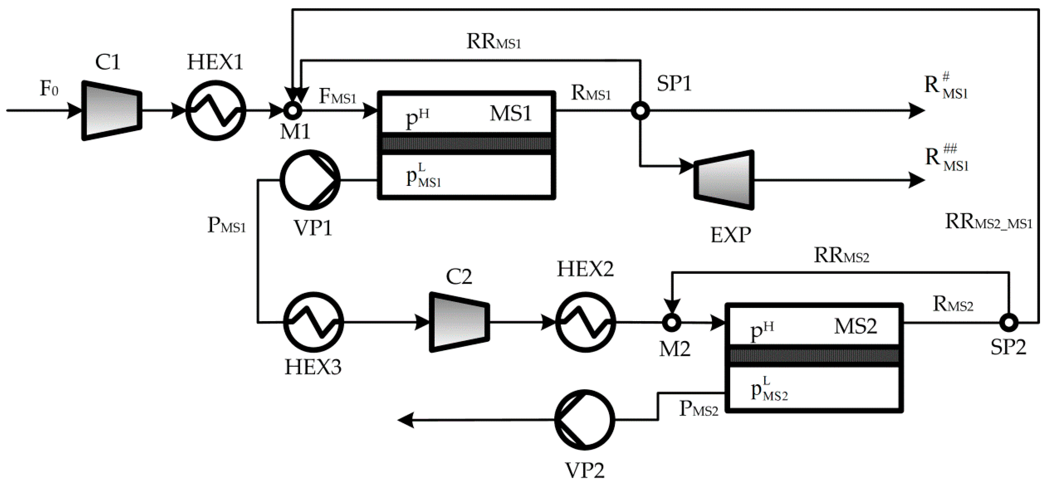
A schematic of the studied two-stage membrane system for hydrogen separation is illustrated in Figure 1. As shown, the feed stream F₀ passes through the compressor C1 and the heat exchanger HEX1 to increase the pressure and to reach the operating temperature, respectively. Afterward, F₀ can be optionally mixed with a fraction of the retentate stream obtained in the first membrane stage MS1 (RR_MS1) and/or the obtained in the second membrane stage MS2 (RR_{MS2_MS1}). Then, the resulting stream F_MS1 is fed to the membrane stage MS1, where it is separated into two streams: a stream that permeates through the membrane (permeate P_MS1) and a stream that is retained by the membrane (retentate R_MS1).

In this study, the driving force for selective permeation can optionally be created by different ways: (a) compressors C1 and/or C2, (b) vacuum pumps VP1 and/or VP2, and (c) a combination of compressors and vacuum pumps. In other words, the ways to create the driving force in each membrane stage will be a result of the optimization problem, specifically through p^H (retentate pressure) and p^L (permeate pressure) which are optimization variables of the process model. (Of course, the driving force also depends on the mole fractions of the components at both membrane sides). For instance, if no vacuum pumps are selected, p^L will be the atmospheric pressure. On the other hand, if no compressors are selected, the driving force will be created by vacuum pumps and p^H will be the atmospheric pressure. Thus, the formulated mathematical model includes the possibility to select (feed and permeate) compression and/or application of vacuum in the permeate streams.

In addition, if the optimal solution selects the inclusion of the compressor C1, the mathematical model has the option to include the expander EXP to recover mechanical power from the retentate stream R_MS1. The model also includes the possibility of recycling part of R_MS2 back to MS2 (RR_MS2) and/or to MS1 (RR_{MS2_MS1}).

As it can be noticed, there are different trade-offs between the pressure ratio (p^H/p^L), the electric power requirement to run compressors and vacuum pumps, and the membrane area. For instance, the higher the pressure ratio, the higher the H₂ purity in the permeate stream and the lower the membrane area but the higher the electric power requirement to run the compressor. The optimal pressure ratio values depend on the relationships between investment and operating costs. However, these trade-offs can show opposite trends if the expander EXP is included into the analysis since the higher the retentate pressure, the higher the amount of power recovered by the expander and, therefore, the lower the total net amount of electric power required to operate the process.

Based on this, it is clear that the finding of optimal solutions could be a difficult and time-consuming task if parametric optimization is employed instead of simultaneous optimization as is proposed in this work. Thus, the relevance of this paper is to simultaneously optimize the trade-offs that are difficult to distinguish at first glance. As a result of the model, the following process design decisions that minimize the total annual cost (capital and operating expenditures) are determined by:

• The way in which the driving force for permeation is created in each membrane stage, i.e., the solution will indicate if the driving force is created by (a) employing compression without applying vacuum, or (b) applying vacuum in the permeate streams without employing compression, or (c) combining both compression and vacuum.
• The inclusion or not of the expansion turbine for power recovery.
• The inclusion or not of (one or more) recycle streams.
• The optimal values of operation pressure, temperature, composition, and flow rate of each process stream.
• The optimal sizes of the process units (membrane areas, heat transfer areas, power capacity of compressors and vacuum pumps).

The specifications of the gas mixture feed and the desired H₂ product purity and H₂ recovery are assumed as model parameters. In this study, H₂ product purity and H₂ recovery target levels of 0.9 and 90%, respectively, are specified, which are typical values for fluid catalytic cracking (FCC) off-gases and other refinery purge streams [31]. As a first approximation, the same polymeric material is considered for both membrane modules and the same permeance values are used in both cases.

3. Process Modeling

3.1. Main Model Assumptions

The following assumptions are considered for modeling the membrane units [20]:

• All the mixture components can permeate through the membrane.
• The operating pressure does not affect the component permeability.
• No pressure drop is considered in the retentate and permeate sides.
• The feed and retentate streams are at the same pressure.
• Plug flow pattern is considered at both sides of the membrane unit.
• Isothermal condition is assumed within the membrane module.
• Fick’s first law is used.

Next, the mathematical model that describes the complete process, including the cost model to calculate the total annual cost in terms of the capital and operating expenditures, is presented.

3.2. Mathematical Model

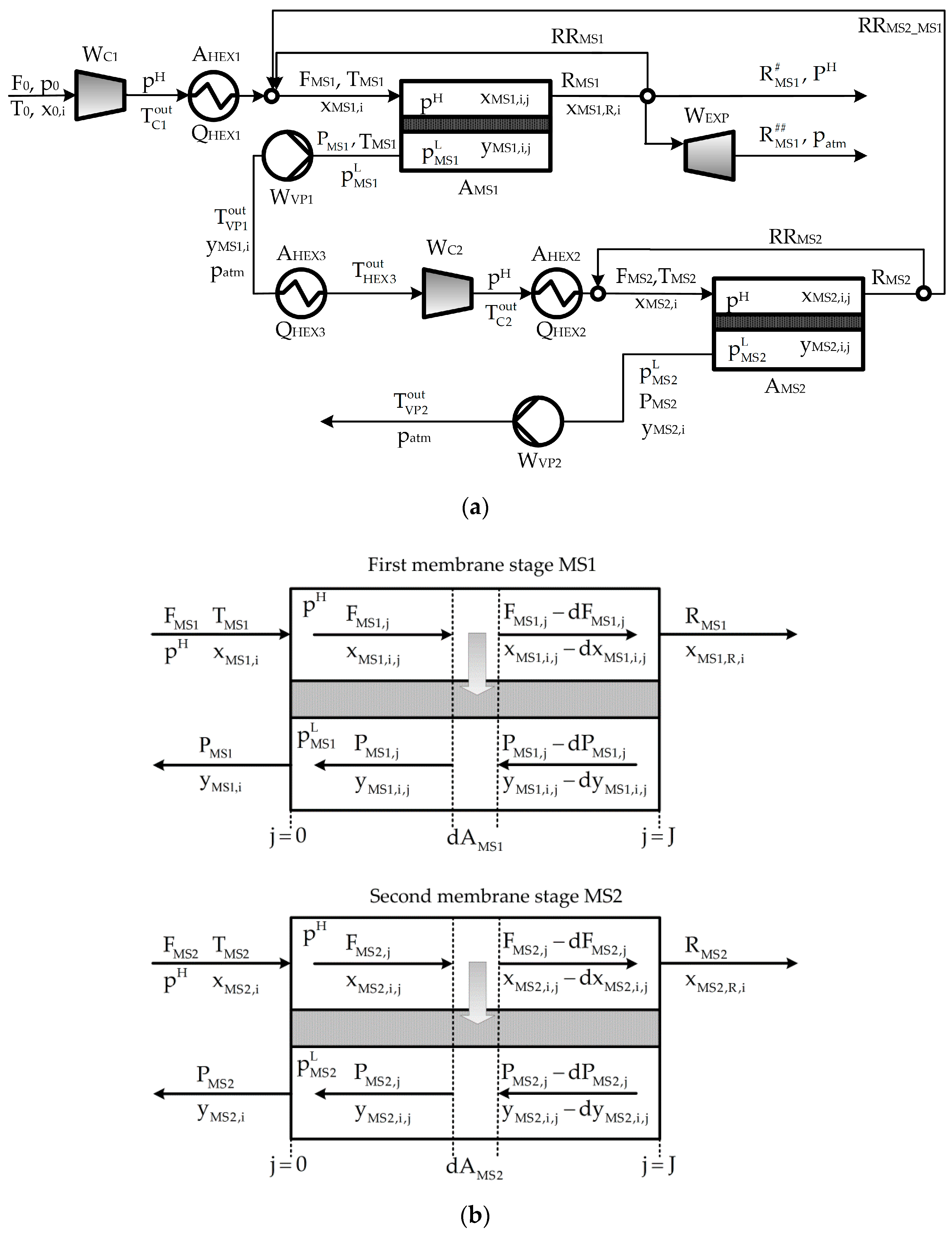
Figure 2 shows a schematic of the whole process and the membrane module, and the nomenclature used to introduce the mathematical model.

3.2.1. Mass Balances

By applying the backward finite difference method (BFDM) to the membrane module MS1 illustrated in Figure 2b, the following set of algebraic equations is obtained:

$$\frac{1}{2}\frac{\left(\mathrm{J}-1\right)}{{\mathrm{A}}_{\mathrm{M}\mathrm{S}1}}\left(-{\mathrm{F}}_{\mathrm{M}\mathrm{S}1,\mathrm{j}}\cdot {\mathrm{x}}_{\mathrm{M}\mathrm{S}1,\mathrm{i},\mathrm{j}}+{\mathrm{F}}_{\mathrm{M}\mathrm{S}1,\mathrm{j}+2}\cdot {\mathrm{x}}_{\mathrm{M}\mathrm{S}1,\mathrm{i},\mathrm{j}+2}\right)+{\mathrm{\xi }}_{\mathrm{i}}\left({\mathrm{p}}^{\mathrm{H}}\cdot {\mathrm{x}}_{\mathrm{M}\mathrm{S}1,\mathrm{i},\mathrm{j}+1}-{\mathrm{p}}_{\mathrm{M}\mathrm{S}1}^{\mathrm{L}}\cdot {\mathrm{y}}_{\mathrm{M}\mathrm{S}1,\mathrm{i},\mathrm{j}+1}\right)=0; \mathrm{j}=0, \forall \mathrm{i}$$

(1)

$$\begin{array}{l}\frac{1}{2}\frac{\left(\mathrm{J}-1\right)}{{\mathrm{A}}_{\mathrm{M}\mathrm{S}1}}\cdot \left({\mathrm{F}}_{\mathrm{M}\mathrm{S}1,\mathrm{j}}\cdot {\mathrm{x}}_{\mathrm{M}\mathrm{S}1,\mathrm{i},\mathrm{j}}-4\cdot {\mathrm{F}}_{\mathrm{M}\mathrm{S}1,\mathrm{j}+1}\cdot {\mathrm{x}}_{\mathrm{M}\mathrm{S}1,\mathrm{i},\mathrm{j}+1}+3\cdot {\mathrm{F}}_{\mathrm{M}\mathrm{S}1,\mathrm{j}+2}\cdot {\mathrm{x}}_{\mathrm{M}\mathrm{S}1,\mathrm{i},\mathrm{j}+2}\right)+\\ {\mathrm{\xi }}_{\mathrm{i}}\cdot \left({\mathrm{p}}^{\mathrm{H}}\cdot {\mathrm{x}}_{\mathrm{M}\mathrm{S}1,\mathrm{i},\mathrm{j}+2}-{\mathrm{p}}_{\mathrm{M}\mathrm{S}1}^{\mathrm{L}}\cdot {\mathrm{y}}_{\mathrm{M}\mathrm{S}1,\mathrm{i},\mathrm{j}+2}\right)=0; \mathrm{j}=0,\dots ,\mathrm{J}-2\end{array}$$

(2)

where ξ_i and A_MS1 refer to the permeance of component i and membrane surface area, respectively. p^H and p^L_MS1 are the operating pressures in the retentate and permeate sides, respectively. The index j refers to a discretization point which varies from 0 to 19 (J = 19, i.e., 20 discretization points is considered).

$${\mathrm{F}}_{\mathrm{M}\mathrm{S}1,\mathrm{j}=0}\cdot {\mathrm{x}}_{\mathrm{M}\mathrm{S}1,\mathrm{i},\mathrm{j}=0}-{\mathrm{F}}_{\mathrm{M}\mathrm{S}1,\mathrm{j}=\mathrm{J}}\cdot {\mathrm{x}}_{\mathrm{M}\mathrm{S}1,\mathrm{i},\mathrm{j}=\mathrm{J}}-{\mathrm{P}}_{\mathrm{M}\mathrm{S}1,\mathrm{j}=0}\cdot {\mathrm{y}}_{\mathrm{M}\mathrm{S}1,\mathrm{i},\mathrm{j}=0}=0; \forall \mathrm{i}$$

(3)

$${\mathrm{F}}_{\mathrm{M}\mathrm{S}1,\mathrm{j}=0}-{\mathrm{F}}_{\mathrm{M}\mathrm{S}1,\mathrm{j}=\mathrm{J}}-{\mathrm{P}}_{\mathrm{M}\mathrm{S}1,\mathrm{j}=0}\hspace{0.17em}=0$$

(4)

$${\displaystyle \sum _{\mathrm{i}}{\mathrm{x}}_{\mathrm{M}\mathrm{S}1,\mathrm{i},\mathrm{j}}}=1;\forall \mathrm{j},\mathrm{i}{=\mathrm{H}}_2{,\mathrm{N}}_2{,\mathrm{CO}}_2,\mathrm{CO}$$

(5)

$${\displaystyle \sum _{\mathrm{i}}{\mathrm{y}}_{\mathrm{M}\mathrm{S}1,\mathrm{i},\mathrm{j}}}=1;\forall \mathrm{j},\mathrm{i}{=\mathrm{H}}_2{,\mathrm{N}}_2{,\mathrm{CO}}_2,\mathrm{CO}$$

(6)

A similar set of constraints is formulated for the second membrane stage MS2.

The mass balances in splitters SP1 and SP2 are expressed as follows:

$${\mathrm{R}}_{\mathrm{M}\mathrm{S}1}=\mathrm{R}{\mathrm{R}}_{\mathrm{M}\mathrm{S}1}+{\mathrm{R}}_{\mathrm{M}\mathrm{S}1}^{\#}+{\mathrm{R}}_{\mathrm{M}\mathrm{S}1}^{\#\#}$$

(7)

$${\mathrm{R}}_{\mathrm{M}\mathrm{S}2}=\mathrm{R}{\mathrm{R}}_{\mathrm{M}\mathrm{S}2}+\mathrm{R}{\mathrm{R}}_{\mathrm{M}\mathrm{S}2\_\mathrm{M}\mathrm{S}1}$$

(8)

3.2.2. Power Requirement

The electric power required by compressors (C1, C2) and vacuum pumps (VP1, VP2) are calculated as follows:

$${\mathrm{W}}_{\mathrm{C}1}=\frac{{\mathrm{F}}_0}{{\mathrm{\eta }}_{\mathrm{C}}}\cdot \left(\frac{\mathrm{\gamma }}{\mathrm{\gamma }-1}\right)\cdot \mathrm{R}\cdot {\mathrm{T}}_0\cdot \left[{\left(\frac{{\mathrm{p}}^{\mathrm{H}}}{{\mathrm{p}}_0}\right)}^{\frac{\mathrm{\gamma }-1}{\mathrm{\gamma }}}-1\right]$$

(9)

$$\frac{{\mathrm{T}}_{\mathrm{C}1}^{\mathrm{o}\mathrm{u}\mathrm{t}}}{{\mathrm{T}}_0}={\left(\frac{{\mathrm{p}}^{\mathrm{H}}}{{\mathrm{p}}_0}\right)}^{\frac{\mathrm{\gamma }-1}{\mathrm{\gamma }}}$$

(10)

$${\mathrm{W}}_{\mathrm{C}2}=\frac{{\mathrm{P}}_{\mathrm{M}\mathrm{S}1}}{{\mathrm{\eta }}_{\mathrm{C}}}\cdot \left(\frac{\mathrm{\gamma }}{\mathrm{\gamma }-1}\right)\cdot \mathrm{R}\cdot {\mathrm{T}}_{\mathrm{H}\mathrm{E}\mathrm{X}3}^{\mathrm{o}\mathrm{u}\mathrm{t}}\cdot \left[{\left(\frac{{\mathrm{p}}^{\mathrm{H}}}{{\mathrm{p}}_0}\right)}^{\frac{\mathrm{\gamma }-1}{\mathrm{\gamma }}}-1\right]$$

(11)

$$\frac{{\mathrm{T}}_{\mathrm{C}2}^{\mathrm{o}\mathrm{u}\mathrm{t}}}{{\mathrm{T}}_{\mathrm{H}\mathrm{E}\mathrm{X}3}^{\mathrm{o}\mathrm{u}\mathrm{t}}}={\left(\frac{{\mathrm{p}}^{\mathrm{H}}}{{\mathrm{p}}_0}\right)}^{\frac{\mathrm{\gamma }-1}{\mathrm{\gamma }}}$$

(12)

The parameters γ, η_c, and P₀ refer, respectively, to the adiabatic expansion coefficient (1.4), efficiency (0.85), and atmospheric pressure (101.32 kPa).

$${\mathrm{W}}_{\mathrm{V}\mathrm{P}1}=\frac{{\mathrm{P}}_{\mathrm{M}\mathrm{S}1}}{{\mathrm{\eta }}_{\mathrm{C}}}\cdot \left(\frac{\mathrm{\gamma }}{\mathrm{\gamma }-1}\right)\cdot \mathrm{R}\cdot {\mathrm{T}}_{\mathrm{M}\mathrm{S}1}\cdot \left[{\left(\frac{{\mathrm{p}}_0}{{\mathrm{p}}_{\mathrm{M}\mathrm{S}1}^{\mathrm{L}}}\right)}^{\frac{\mathrm{\gamma }-1}{\mathrm{\gamma }}}-1\right]$$

(13)

$$\frac{{\mathrm{T}}_{\mathrm{V}\mathrm{P}1}^{\mathrm{o}\mathrm{u}\mathrm{t}}}{{\mathrm{T}}_{\mathrm{M}\mathrm{S}1}}={\left(\frac{{\mathrm{p}}_0}{{\mathrm{p}}_{\mathrm{M}\mathrm{S}1}^{\mathrm{L}}}\right)}^{\frac{\mathrm{\gamma }-1}{\mathrm{\gamma }}}$$

(14)

$${\mathrm{W}}_{\mathrm{V}\mathrm{P}2}=\frac{{\mathrm{P}}_{\mathrm{M}\mathrm{S}2}}{{\mathrm{\eta }}_{\mathrm{C}}}\cdot \left(\frac{\mathrm{\gamma }}{\mathrm{\gamma }-1}\right)\cdot \mathrm{R}\cdot {\mathrm{T}}_{\mathrm{M}\mathrm{S}2}\cdot \left[{\left(\frac{{\mathrm{p}}_0}{{\mathrm{p}}_{\mathrm{M}\mathrm{S}2}^{\mathrm{L}}}\right)}^{\frac{\mathrm{\gamma }-1}{\mathrm{\gamma }}}-1\right]$$

(15)

$$\frac{{\mathrm{T}}_{\mathrm{V}\mathrm{P}2}^{\mathrm{o}\mathrm{u}\mathrm{t}}}{{\mathrm{T}}_{\mathrm{M}\mathrm{S}2}}={\left(\frac{{\mathrm{p}}_0}{{\mathrm{p}}_{\mathrm{M}\mathrm{S}2}^{\mathrm{L}}}\right)}^{\frac{\mathrm{\gamma }-1}{\mathrm{\gamma }}}$$

(16)

Finally, the power W_EXP recovered in the expander (isothermal expansion) is given by Equation (17):

$${\mathrm{W}}_{\mathrm{E}\mathrm{X}\mathrm{P}}=\frac{{\mathrm{R}}_{\mathrm{M}\mathrm{S}1}^{\#\#}}{{\mathrm{\eta }}_{\mathrm{E}}}\cdot \mathrm{R}\cdot {\mathrm{T}}_{\mathrm{M}\mathrm{S}1}\cdot \ln \left(\frac{{\mathrm{p}}^{\mathrm{H}}}{{\mathrm{p}}_{\mathrm{a}\mathrm{t}\mathrm{m}}}\right)$$

(17)

As mentioned earlier, the model was developed in such a way that the expander can be selected or removed from the optimal solution, depending on the optimal flow rate values in the splitter SP1 (Equation (7)). For instance, if the optimal value of R_MS1^## in Equation (7) is equal to 0, then the expander is removed and no electric power is recovered.

3.2.3. Energy Balances and Transfer Areas of Heat Exchangers

The energy balances in the heat exchangers and the corresponding heat transfer areas are calculated by Equations (18)–(26):

$${\mathrm{F}}_0\cdot {\mathrm{c}}_{\mathrm{P}}^{\mathrm{g}}\cdot \left({\mathrm{T}}_{\mathrm{C}1}^{\mathrm{o}\mathrm{u}\mathrm{t}}-{\mathrm{T}}_{\mathrm{M}\mathrm{S}1}\right)={\mathrm{n}}_{\mathrm{H}\mathrm{E}\mathrm{X}1,\mathrm{c}\mathrm{w}}\cdot {\mathrm{c}}_{\mathrm{P}}^{\mathrm{c}\mathrm{w}}\cdot \left({\mathrm{T}}_{\mathrm{H}\mathrm{E}\mathrm{X}1,\mathrm{c}\mathrm{w}}^{\mathrm{o}\mathrm{u}\mathrm{t}}-{\mathrm{T}}_{\mathrm{H}\mathrm{E}\mathrm{X}1,\mathrm{c}\mathrm{w}}^{\mathrm{i}\mathrm{n}\mathrm{l}}\right)$$

(18)

$${\mathrm{P}}_{\mathrm{M}\mathrm{S}1}\cdot {\mathrm{c}}_{\mathrm{P}}^{\mathrm{g}}\cdot \left({\mathrm{T}}_{\mathrm{C}2}^{\mathrm{o}\mathrm{u}\mathrm{t}}-{\mathrm{T}}_{\mathrm{M}\mathrm{S}2}\right)={\mathrm{n}}_{\mathrm{H}\mathrm{E}\mathrm{X}2,\mathrm{c}\mathrm{w}}\cdot {\mathrm{c}}_{\mathrm{P}}^{\mathrm{c}\mathrm{w}}\cdot \left({\mathrm{T}}_{\mathrm{H}\mathrm{E}\mathrm{X}2,\mathrm{c}\mathrm{w}}^{\mathrm{o}\mathrm{u}\mathrm{t}}-{\mathrm{T}}_{\mathrm{H}\mathrm{E}\mathrm{X}2,\mathrm{c}\mathrm{w}}^{\mathrm{i}\mathrm{n}\mathrm{l}}\right)$$

(19)

$${\mathrm{P}}_{\mathrm{M}\mathrm{S}1}\cdot {\mathrm{c}}_{\mathrm{P}}^{\mathrm{g}}\cdot \left({\mathrm{T}}_{\mathrm{V}\mathrm{P}1}^{\mathrm{o}\mathrm{u}\mathrm{t}}-{\mathrm{T}}_{\mathrm{H}\mathrm{E}\mathrm{X}3}^{\mathrm{o}\mathrm{u}\mathrm{t}}\right)={\mathrm{n}}_{\mathrm{H}\mathrm{E}\mathrm{X}3,\mathrm{c}\mathrm{w}}\cdot {\mathrm{c}}_{\mathrm{P}}^{\mathrm{c}\mathrm{w}}\cdot \left({\mathrm{T}}_{\mathrm{H}\mathrm{E}\mathrm{X}3,\mathrm{c}\mathrm{w}}^{\mathrm{o}\mathrm{u}\mathrm{t}}-{\mathrm{T}}_{\mathrm{H}\mathrm{E}\mathrm{X}3,\mathrm{c}\mathrm{w}}^{\mathrm{i}\mathrm{n}\mathrm{l}}\right)$$

(20)

$${\mathrm{A}}_{\mathrm{H}\mathrm{E}\mathrm{X}1}=\frac{{\mathrm{F}}_0\cdot {\mathrm{c}}_{\mathrm{P}}^{\mathrm{g}}\cdot \left({\mathrm{T}}_{\mathrm{C}1}^{\mathrm{o}\mathrm{u}\mathrm{t}}-{\mathrm{T}}_{\mathrm{M}\mathrm{S}1}\right)}{\mathrm{U}\cdot \mathrm{L}\mathrm{M}\mathrm{T}{\mathrm{D}}_{\mathrm{H}\mathrm{E}\mathrm{X}1}}$$

(21)

$${\mathrm{A}}_{\mathrm{H}\mathrm{E}\mathrm{X}2}=\frac{{\mathrm{P}}_{\mathrm{M}\mathrm{S}1}\cdot {\mathrm{c}}_{\mathrm{P}}^{\mathrm{g}}\cdot \left({\mathrm{T}}_{\mathrm{C}2}^{\mathrm{o}\mathrm{u}\mathrm{t}}-{\mathrm{T}}_{\mathrm{M}\mathrm{S}2}\right)}{\mathrm{U}\cdot \mathrm{L}\mathrm{M}\mathrm{T}{\mathrm{D}}_{\mathrm{H}\mathrm{E}\mathrm{X}2}}$$

(22)

$${\mathrm{A}}_{\mathrm{H}\mathrm{E}\mathrm{X}3}=\frac{{\mathrm{P}}_{\mathrm{M}\mathrm{S}1}\cdot {\mathrm{c}}_{\mathrm{P}}^{\mathrm{g}}\cdot \left({\mathrm{T}}_{\mathrm{V}\mathrm{P}1}^{\mathrm{o}\mathrm{u}\mathrm{t}}-{\mathrm{T}}_{\mathrm{H}\mathrm{E}\mathrm{X}3}^{\mathrm{o}\mathrm{u}\mathrm{t}}\right)}{\mathrm{U}\cdot \mathrm{L}\mathrm{M}\mathrm{T}{\mathrm{D}}_{\mathrm{H}\mathrm{E}\mathrm{X}3}}$$

(23)

$$\mathrm{L}\mathrm{M}\mathrm{T}{\mathrm{D}}_{\mathrm{H}\mathrm{E}\mathrm{X}1}=\frac{\left({\mathrm{T}}_{\mathrm{C}1}^{\mathrm{o}\mathrm{u}\mathrm{t}}-{\mathrm{T}}_{\mathrm{H}\mathrm{E}\mathrm{X}1,\mathrm{c}\mathrm{w}}^{\mathrm{o}\mathrm{u}\mathrm{t}}\right)-\left({\mathrm{T}}_{\mathrm{M}\mathrm{S}1}-{\mathrm{T}}_{\mathrm{H}\mathrm{E}\mathrm{X}1,\mathrm{c}\mathrm{w}}^{\mathrm{i}\mathrm{n}\mathrm{l}}\right)}{\ln \frac{\left({\mathrm{T}}_{\mathrm{C}1}^{\mathrm{o}\mathrm{u}\mathrm{t}}-{\mathrm{T}}_{\mathrm{H}\mathrm{E}\mathrm{X}1,\mathrm{c}\mathrm{w}}^{\mathrm{o}\mathrm{u}\mathrm{t}}\right)}{\left({\mathrm{T}}_{\mathrm{M}\mathrm{S}1}-{\mathrm{T}}_{\mathrm{H}\mathrm{E}\mathrm{X}1,\mathrm{c}\mathrm{w}}^{\mathrm{i}\mathrm{n}\mathrm{l}}\right)}}$$

(24)

$$\mathrm{L}\mathrm{M}\mathrm{T}{\mathrm{D}}_{\mathrm{H}\mathrm{E}\mathrm{X}2}=\frac{\left({\mathrm{T}}_{\mathrm{C}2}^{\mathrm{o}\mathrm{u}\mathrm{t}}-{\mathrm{T}}_{\mathrm{H}\mathrm{E}\mathrm{X}2,\mathrm{c}\mathrm{w}}^{\mathrm{o}\mathrm{u}\mathrm{t}}\right)-\left({\mathrm{T}}_{\mathrm{M}\mathrm{S}2}-{\mathrm{T}}_{\mathrm{H}\mathrm{E}\mathrm{X}2,\mathrm{c}\mathrm{w}}^{\mathrm{i}\mathrm{n}\mathrm{l}}\right)}{\ln \frac{\left({\mathrm{T}}_{\mathrm{C}2}^{\mathrm{o}\mathrm{u}\mathrm{t}}-{\mathrm{T}}_{\mathrm{H}\mathrm{E}\mathrm{X}2,\mathrm{c}\mathrm{w}}^{\mathrm{o}\mathrm{u}\mathrm{t}}\right)}{\left({\mathrm{T}}_{\mathrm{M}\mathrm{S}2}-{\mathrm{T}}_{\mathrm{H}\mathrm{E}\mathrm{X}2,\mathrm{c}\mathrm{w}}^{\mathrm{i}\mathrm{n}\mathrm{l}}\right)}}$$

(25)

$$\mathrm{L}\mathrm{M}\mathrm{T}{\mathrm{D}}_{\mathrm{H}\mathrm{E}\mathrm{X}3}=\frac{\left({\mathrm{T}}_{\mathrm{V}\mathrm{P}1}^{\mathrm{o}\mathrm{u}\mathrm{t}}-{\mathrm{T}}_{\mathrm{H}\mathrm{E}\mathrm{X}3,\mathrm{c}\mathrm{w}}^{\mathrm{o}\mathrm{u}\mathrm{t}}\right)-\left({\mathrm{T}}_{\mathrm{H}\mathrm{E}\mathrm{X}3}^{\mathrm{o}\mathrm{u}\mathrm{t}}-{\mathrm{T}}_{\mathrm{H}\mathrm{E}\mathrm{X}3,\mathrm{c}\mathrm{w}}^{\mathrm{i}\mathrm{n}\mathrm{l}}\right)}{\ln \frac{\left({\mathrm{T}}_{\mathrm{V}\mathrm{P}1}^{\mathrm{o}\mathrm{u}\mathrm{t}}-{\mathrm{T}}_{\mathrm{H}\mathrm{E}\mathrm{X}3,\mathrm{c}\mathrm{w}}^{\mathrm{o}\mathrm{u}\mathrm{t}}\right)}{\left({\mathrm{T}}_{\mathrm{H}\mathrm{E}\mathrm{X}3}^{\mathrm{o}\mathrm{u}\mathrm{t}}-{\mathrm{T}}_{\mathrm{H}\mathrm{E}\mathrm{X}3,\mathrm{c}\mathrm{w}}^{\mathrm{i}\mathrm{n}\mathrm{l}}\right)}}$$

(26)

The parameter U refers to the overall heat transfer coefficient, which is assumed to be 277.7 W·m⁻²·K⁻¹ for all heat exchangers.

3.2.4. Connecting Constraints

The following constraints are used to relate model variables defined inside and outside of the membrane module MS1:

$${\mathrm{F}}_{\mathrm{M}\mathrm{S}1}={\mathrm{F}}_{\mathrm{M}\mathrm{S}1,\mathrm{j}=0}$$

(27)

$${\mathrm{x}}_{\mathrm{M}\mathrm{S}1,\mathrm{i}}={\mathrm{x}}_{\mathrm{M}\mathrm{S}1,\mathrm{i},\mathrm{j}=0}$$

(28)

$${\mathrm{F}}_{\mathrm{M}\mathrm{S}1,\mathrm{j}=\mathrm{J}}={\mathrm{R}}_{\mathrm{M}\mathrm{S}1}$$

(29)

$${\mathrm{x}}_{\mathrm{M}\mathrm{S}1,\mathrm{i},\mathrm{j}=\mathrm{J}}={\mathrm{x}}_{\mathrm{M}\mathrm{S}1,\mathrm{R},\mathrm{i}}$$

(30)

$${\mathrm{P}}_{\mathrm{M}\mathrm{S}1}={\mathrm{P}}_{\mathrm{M}\mathrm{S}1,\mathrm{j}=0}$$

(31)

$${\mathrm{y}}_{\mathrm{M}\mathrm{S}1,\mathrm{i}}={\mathrm{y}}_{\mathrm{M}\mathrm{S}1,\mathrm{i},\mathrm{j}=0}$$

(32)

Similar constraints are considered for the second membrane stage MS2.

3.2.5. Performance Variables

The total membrane area (TMA) and the total heat transfer area (THTA) are calculated by Equations (33) and (34), respectively:

$$\mathrm{T}\mathrm{M}\mathrm{A}={\mathrm{A}}_{\mathrm{M}\mathrm{S}1}+{\mathrm{A}}_{\mathrm{M}\mathrm{S}2}$$

(33)

$$\mathrm{T}\mathrm{H}\mathrm{T}\mathrm{A}={\mathrm{A}}_{\mathrm{H}\mathrm{E}\mathrm{X}1}+{\mathrm{A}}_{\mathrm{H}\mathrm{E}\mathrm{X}2}+{\mathrm{A}}_{\mathrm{H}\mathrm{E}\mathrm{X}3}$$

(34)

The total and net power requirements (TW and TNW, respectively) are calculated as follows:

$$\mathrm{T}\mathrm{W}={\mathrm{W}}_{\mathrm{C}1}+{\mathrm{W}}_{\mathrm{C}2}+{\mathrm{W}}_{\mathrm{V}\mathrm{P}1}+{\mathrm{W}}_{\mathrm{V}\mathrm{P}2}$$

(35)

$$\mathrm{T}\mathrm{N}\mathrm{W}=\mathrm{T}\mathrm{W}-{\mathrm{W}}_{\mathrm{E}\mathrm{X}\mathrm{P}}$$

(36)

3.2.6. Cost Model

The total annual cost (TAC, in M$·year⁻¹), capital expenditures (CAPEX, in M$), annualized capital expenditures (annCAPEX, in M$·year⁻¹), and operating expenditures (OPEX, in M$·year⁻¹) are calculated by Equations (37)–(41).

$$\mathrm{T}\mathrm{A}\mathrm{C}=\mathrm{a}\mathrm{n}\mathrm{n}\mathrm{C}\mathrm{A}\mathrm{P}\mathrm{E}\mathrm{X}+\mathrm{O}\mathrm{P}\mathrm{E}\mathrm{X}$$

(37)

$$\mathrm{a}\mathrm{n}\mathrm{n}\mathrm{C}\mathrm{A}\mathrm{P}\mathrm{E}\mathrm{X}=\mathrm{C}\mathrm{R}\mathrm{F}\cdot \mathrm{C}\mathrm{A}\mathrm{P}\mathrm{E}\mathrm{X}$$

(38)

$$\mathrm{C}\mathrm{R}\mathrm{F}=\frac{\mathrm{i}\cdot {\left(1+\mathrm{i}\right)}^{\mathrm{n}}}{{\left(1+\mathrm{i}\right)}^{\mathrm{n}}-1}$$

(39)

$$\mathrm{C}\mathrm{A}\mathrm{P}\mathrm{E}\mathrm{X}={\mathrm{f}}_1\cdot {\mathrm{C}}_{\mathrm{I}\mathrm{N}\mathrm{V}}$$

(40)

$$\mathrm{O}\mathrm{P}\mathrm{E}\mathrm{X}={\mathrm{f}}_2\cdot {\mathrm{C}}_{\mathrm{I}\mathrm{N}\mathrm{V}}+{\mathrm{f}}_3\cdot \mathrm{O}\mathrm{L}\mathrm{M}+{\mathrm{f}}_4\cdot {\mathrm{C}}_{\mathrm{R}\mathrm{M}}$$

(41)

In Equation (41), OLM accounts for manpower and maintenance costs. A detailed calculation of the economic factors f₁ (4.98), f₂ (0.464), f₃ (2.45), and f₄ (1.055) can be found in [20], which were estimated based on the guidelines given in [32,33].

The total investment cost (C_INV, in M$) is calculated by Equation (42), where the investment costs of the individual process units are estimated by Equations (43)–(47):

$${\mathrm{C}}_{\mathrm{I}\mathrm{N}\mathrm{V}}={\mathrm{I}}_{\mathrm{C}1}+{\mathrm{I}}_{\mathrm{C}2}+{\mathrm{I}}_{\mathrm{V}\mathrm{P}1}+{\mathrm{I}}_{\mathrm{V}\mathrm{P}2}+{\mathrm{I}}_{\mathrm{H}\mathrm{E}\mathrm{X}1}+{\mathrm{I}}_{\mathrm{H}\mathrm{E}\mathrm{X}2}+{\mathrm{I}}_{\mathrm{H}\mathrm{E}\mathrm{X}3}+{\mathrm{I}}_{\mathrm{M}\mathrm{S}1}+{\mathrm{I}}_{\mathrm{M}\mathrm{S}2}$$

(42)

$${\mathrm{I}}_{\mathrm{H}\mathrm{E}\mathrm{X}}=0.357\cdot {\left(\frac{{\mathrm{A}}_{\mathrm{H}\mathrm{E}\mathrm{X}}}{929}\right)}^{0.6};\mathrm{HEX}:\mathrm{HEX}1,\mathrm{HEX}2,\mathrm{HEX}3$$

(43)

$${\mathrm{I}}_{\mathrm{C}}=2.788\cdot {\left(\frac{{\mathrm{W}}_{\mathrm{C}}}{2000}\right)}^{0.6};\mathrm{C}:\mathrm{C}1,\mathrm{C}2$$

(44)

$${\mathrm{I}}_{\mathrm{E}\mathrm{X}\mathrm{P}}=2.788\cdot {\left(\frac{{\mathrm{W}}_{\mathrm{E}\mathrm{X}\mathrm{P}}}{2000}\right)}^{0.6}$$

(45)

$${\mathrm{I}}_{\mathrm{V}\mathrm{P}}=2.25\times 10^{-6}\cdot {\mathrm{W}}_{\mathrm{V}\mathrm{P}};\mathrm{VP}:\mathrm{VP}1,\mathrm{VP}2$$

(46)

$${\mathrm{I}}_{\mathrm{M}\mathrm{S}}=52.8\times 10^{-6}\cdot {\mathrm{A}}_{\mathrm{MS}}+0.249\cdot {\left(\frac{0.1}{55}\cdot {\mathrm{p}}^{\mathrm{H}}\right)}^{0.875}\cdot {\left(\frac{{\mathrm{A}}_{\mathrm{M}\mathrm{S}}}{2000}\right)}^{0.7};\mathrm{MS}:\mathrm{MS}1,\mathrm{MS}2$$

(47)

The raw material cost (C_RM, in M$·year⁻¹) used in Equation (41) is calculated by Equation (48). It depends on the cost of electricity (EP), cooling water (CW), and membrane replacement (MR), which are expressed by Equations (49)–(51), respectively:

$${\mathrm{C}}_{\mathrm{R}\mathrm{M}}={\mathrm{C}}_{\mathrm{E}\mathrm{P}}+{\mathrm{C}}_{\mathrm{C}\mathrm{W}}+{\mathrm{C}}_{\mathrm{M}\mathrm{R}}$$

(48)

$${\mathrm{C}}_{\mathrm{E}\mathrm{P}}=\mathrm{c}\mathrm{r}{\mathrm{u}}_{\mathrm{E}\mathrm{P}}\cdot \mathrm{T}\mathrm{N}\mathrm{W}\cdot \mathrm{O}\mathrm{T}$$

(49)

$${\mathrm{C}}_{\mathrm{C}\mathrm{W}}=\mathrm{c}\mathrm{r}{\mathrm{u}}_{\mathrm{C}\mathrm{W}}\cdot {\mathrm{F}}_{\mathrm{C}\mathrm{W}}\cdot 1.8\times {10}^{-2}\cdot (3600\cdot \mathrm{O}\mathrm{T})$$

(50)

$${\mathrm{C}}_{\mathrm{M}\mathrm{R}}=0.2\cdot \mathrm{c}\mathrm{r}{\mathrm{u}}_{\mathrm{M}\mathrm{R}}\cdot ({\mathrm{A}}_{\mathrm{M}\mathrm{S}1}+{\mathrm{A}}_{\mathrm{M}\mathrm{S}2})$$

(51)

where the unitary costs cru_EP, cru_cw, and cru_MR are, respectively, 0.072 $·kW⁻¹, 0.051 $·kg⁻¹, and 10.0 $·m⁻². An operation period (OT) of 6570 h·year⁻¹ was considered.

The numerical values of the model parameters used in this optimization study are taken from Zarca et al. [30], which are listed in

Table 1. Numerical values of model parameters [30].

Parameter	Value
Feed specification
Flow rate, kmol·h−1	100
Temperature, K	313.15
Pressure, kPa	101.32
Composition (mole fraction)
CO2	0.04
CO	0.16
H2	0.18
N2	0.62
Membrane material (Polymer)
Permeance, mole·m−2·s−1·MPa−1)
CO2	8.444 × 10−3
CO	7.457 × 10−4
H2	2.871 × 10−2
N2	4.078 × 10−4

.

The resulting NLP optimization model was implemented in GAMS and solved with CONOPT.

4. Results and Discussion

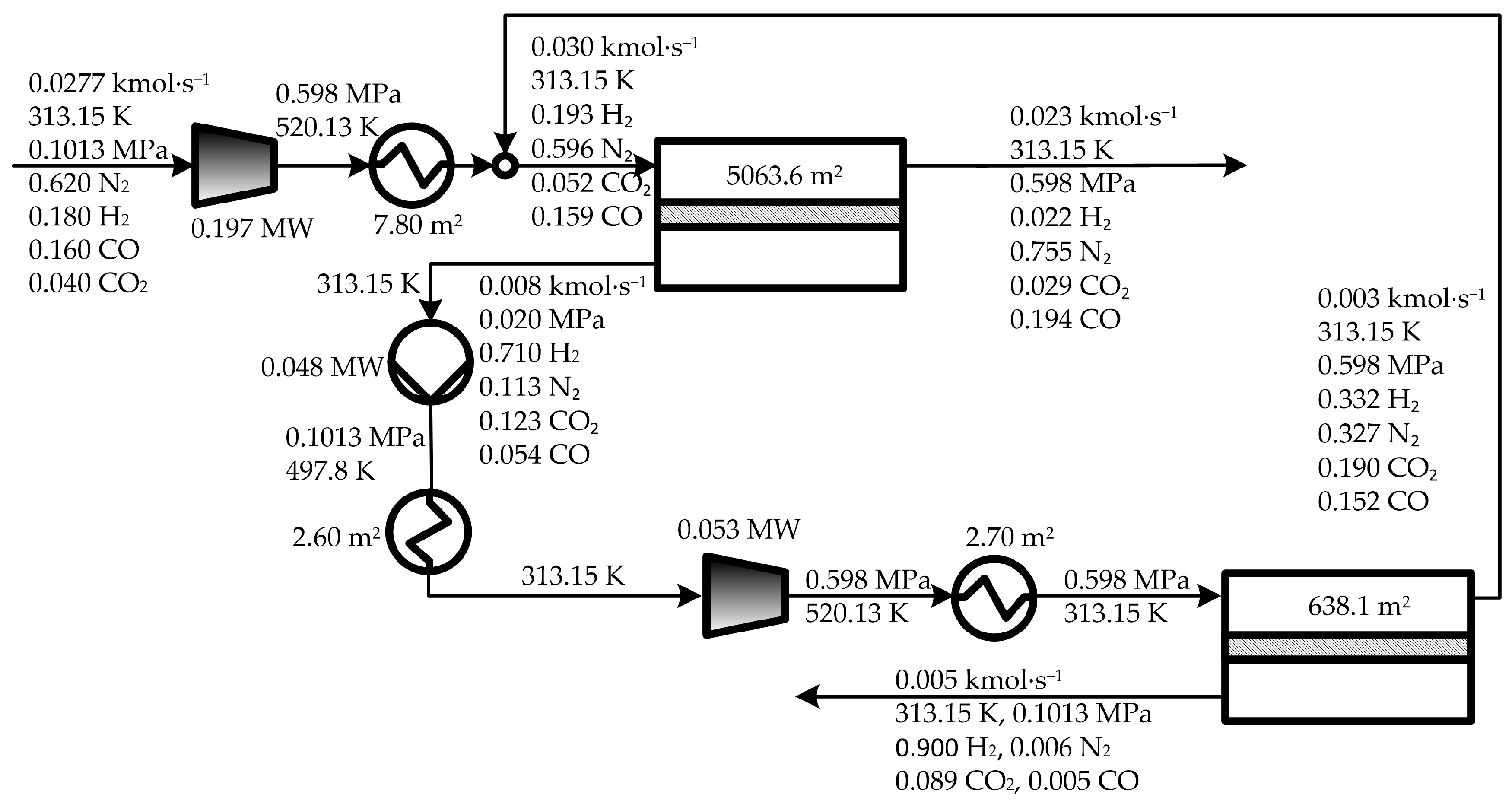
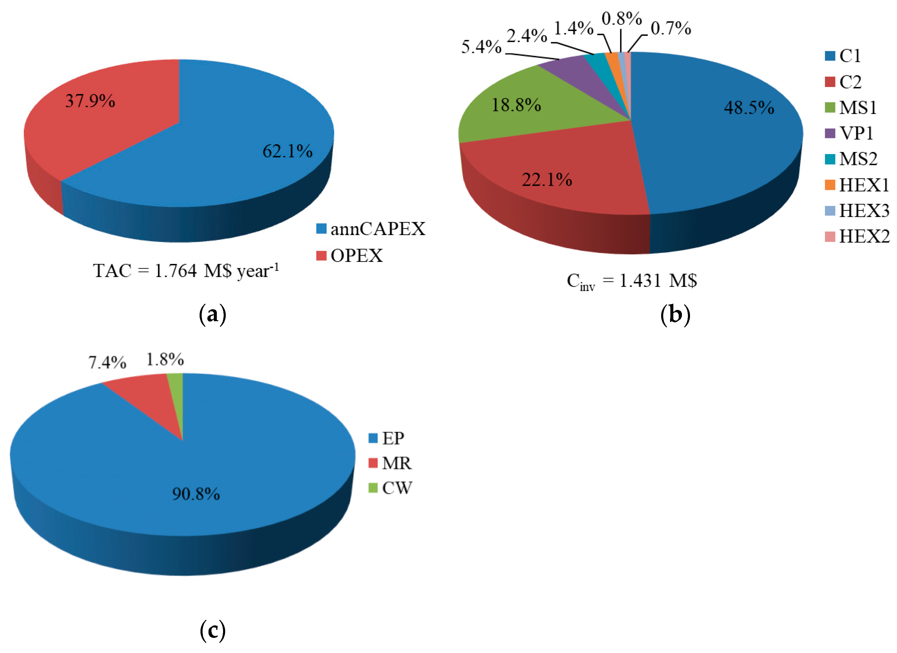
Figure 3 illustrates the optimal process configuration obtained by solving the stated optimization problem, which is hereafter named solution ‘OPT’. Figure 4 shows the percentage contribution of the annualized CAPEX (annCAPEX) and OPEX to the TAC value (Figure 4a), the percentage contribution of each process unit to the total equipment acquisition investment C_INV (Figure 4b), and the percentage contribution of the electric cost, cooling water cost, and membrane replacement cost to the total utility cost (Figure 4c).

As shown in Figure 3, the optimal configuration involves two compressors (C1 and C2) and one vacuum pump (VP1). As the optimal value of R_EMS1 is equal to 0, the expander was excluded from the optimal configuration. Figure 4a shows that the minimum TAC value is 1.764 M$·year⁻¹, where the annCAPEX contribution is more significant than the OPEX contribution (62% vs. 38%).

Figure 3 also shows that the optimal solution OPT requires 5701.7 m² of membrane area (5063.6 m² in the first stage and 638.1 m² in the second one) which, according to Figure 4b, represents 21.1% of the total equipment acquisition cost C_INV (0.303 of 1.431 M$, see

Table 2. Comparison of the optimal cost values of the three solutions OPT, SUBOPT1, and SUBOPT2.

	Optimal Sol. OPT	Sub-Optimal Sol. SUBOPT1	Sub-Optimal Sol. SUBOPT2
TAC (M$·year−1)	1.764	2.038	2.182
OPEX (M$·year−1)	1.095	1.262	1.272
annCAPEX (M$·year−1)	0.669	0.776	0.911
CINV (M$)	1.431	1.661	1.948
C1	0.694	0.916	0.642
C2	0.316	0.480	0.299
AMS1	0.269	0.214	0.344
VP1	0.077	0.0	0.080
AMS2	0.034	0.015	0.040
HEX1	0.020	0.022	0.020
HEX2	0.011	0.013	0.010
HEX3	0.010	0.0	0.010
VP2	0.0	0.0	7.96 × 10−3
EXP	0.0	0.0	0.494
CRM (M$·year−1)	0.155	0.211	0.094
EP	0.141	0.198	0.077
MR	0.011	8.61 × 10−3	0.014
CW	2.79 × 10−3	3.90 × 10−3	2.76 × 10−3

). In the first membrane stage, the feed compressor C1 requires 0.197 MW and the vacuum pump VP1 requires 0.048 MW, leading to an operating pressure ratio of 29.9 (0.598/0.020). In the second membrane stage, the electric power required in the compressor C2 for compressing the permeate obtained in the first stage is 0.053 MW. Thus, the required total electric power capacity to run the process is 0.298 MW, which represents 75.9% of the C_INV (1.087 of 1.431 M$, see Table 2).

Regarding heat transfer requirements, the heat exchangers require in total 13.1 m² of heat transfer area, which represent only 2.9% of the C_INV (0.041 of 1.430 M$, see Table 2). The results presented in Figure 4b show that the compressor C1 is the largest contributor to the C_INV, followed by the compressor C2 and the membrane area A_MS1 of the first stage, contributing with 48.5%, 22.1%, and 18.8%, respectively. Clearly, in each membrane stage, the compressor is significantly more expensive than the membrane itself (0.694 vs. 0.269 M$ in the first stage, and 0.316 vs. 0.034 M$ in the second one, see Table 2).

Regarding the optimal distribution of the total utility cost C_RM, it can be seen in Figure 4c that the cost for electric power demand C_EP is the largest contributor to C_RM with 90.8%, followed by the cost for membrane replacement C_MR with 7.3%. The contribution of the cost associated to the cooling water C_CW is insignificant as it represents only 1.7% of the C_RM value.

Figure 5 shows the optimal composition profiles of all the components in the retentate and permeate streams along the membrane length (which is represented by the discretization points) of the permeation stages MS1 and MS2. In this separation, the permeate profile is the most interesting profile to analyze because it concentrates H₂, which is the desired component in the product stream.

It can be observed in Figure 5a that the H₂ mole fraction in the permeate stream in the first membrane increases from 0.370 at the discretization point j = 19 (at the feed exit) to 0.710 at the discretization point j = 0 (where the permeate stream leaves the membrane module MS1). Similarly, Figure 5b shows how the H₂ mole fraction in the permeate stream in the second membrane increases from 0.813 at the discretization point j = 19 to 0.90 at j = 0 (where the desired design specifications of 0.90 H₂ purity and 90% H₂ recovery are achieved). Figure 5c,d show the mole fraction profiles of the components in the retentate streams in MS1 and MS2, respectively, which flow in opposite direction to the permeate streams. The H₂ mole fraction in the retentate stream in MS2 (Figure 5d) reaches the lowest value of 0.363 at the discretization point j = 19 i.e., where the H₂ mole fraction in the permeate stream also reaches its lowest value (0.813). Thus, as the retentate flows inside the membrane module, its H₂ mole fraction decreases from the highest value of 0.71 to the lowest value of 0.363. Finally, it can be clearly observed in Figure 5c,d that the CO₂, CO, and N₂ mole fractions increase as the H₂ mole fraction in the retentate stream decreases.

4.1. Comparison of Optimal and Sub-Optimal Solutions

In order to investigate how the optimal solution changes if other ways to create the driving force for permeation are applied, and if the expander is forced to be part of the process configuration, the same process optimization model is solved for the following cases:

• The driving forces are created by compression of the feed and permeate streams only. To do this, the (low) pressures in the permeate streams were set to the atmospheric pressure. The optimal solution obtained for this case is shown in Figure 6 and Figure 7, and is hereafter named ‘SUBOPT1’.
• The expander is included in the process configuration. To do this, the flow rate R_MS1^## in Equation (7) (mass balance in the splitter SP1) is set to zero. The optimal solution obtained for this case is illustrated in Figure 8 and Figure 9, and is hereafter named ‘SUBOPT2’.

Both solutions SUBOPT1 and SUBOPT2 are sub-optimal solutions compared to the optimal solution OPT.

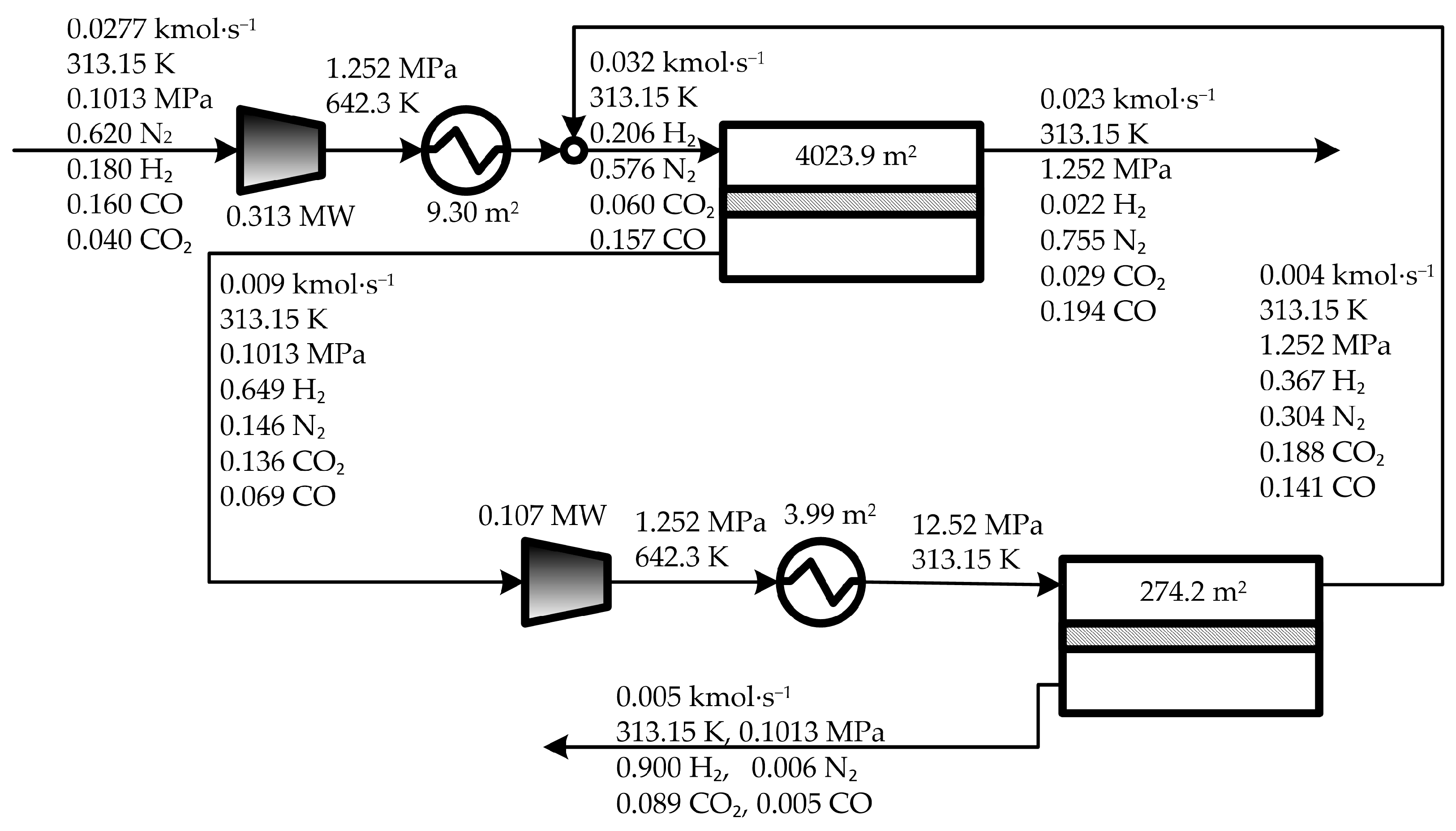
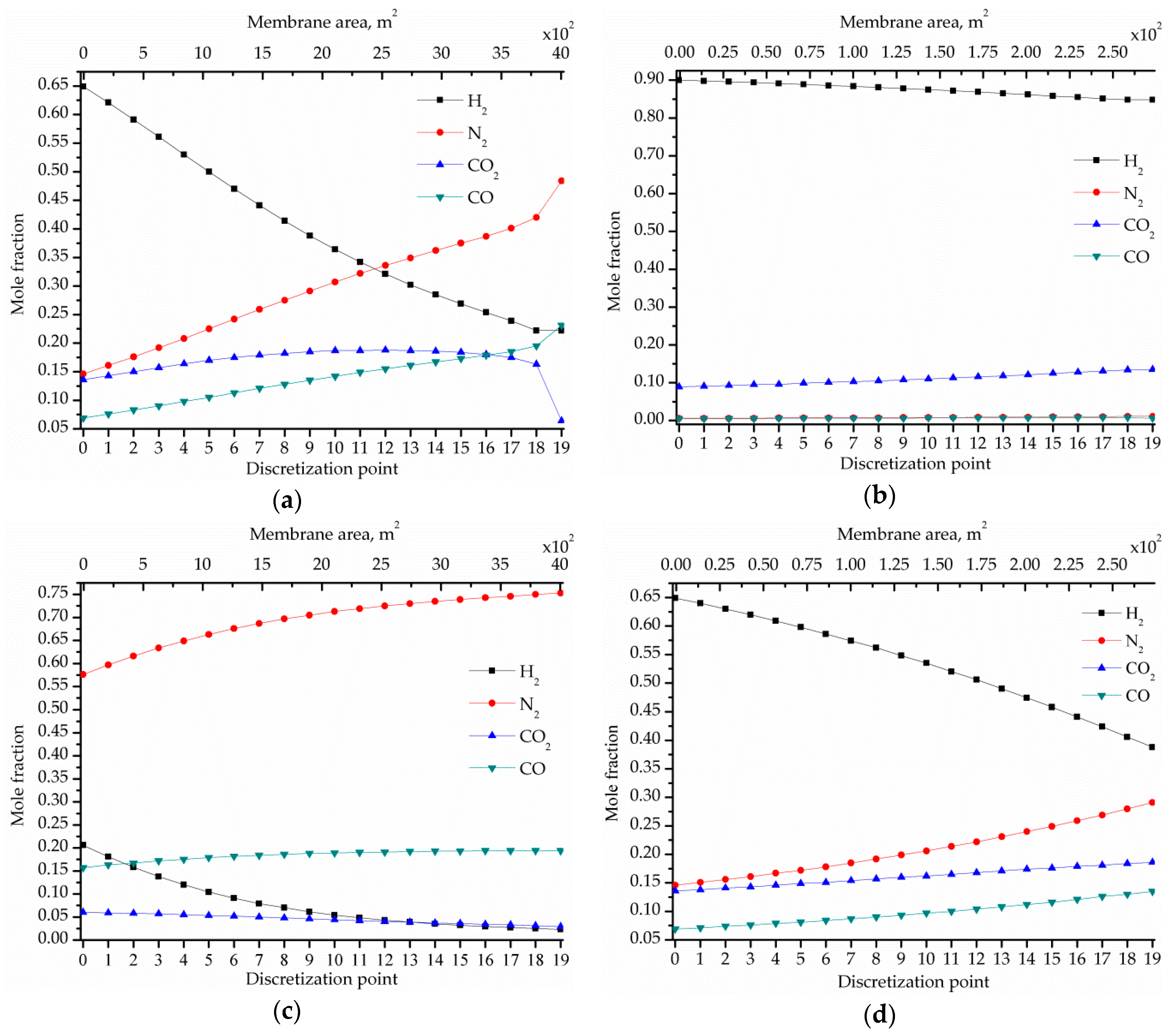
Table 2 compares the costs obtained for these three solutions. The comparison shows that the TAC value obtained for SUBOP1 is 15.5% higher than that obtained for OPT (2.038 vs. 1.764 M$·year⁻¹) as consequence of the increase of both OPEX by 15.2% (from 1.095 to 1.262 M$·year⁻¹) and the annCAPEX by 16.1% (from 0.669 to 0.776 M$·year⁻¹). Also, it can be seen in Figure 6 that the total membrane area required in SUBOP1 is 24.6% lower than that required in OPT (4298.07 vs. 5701.67 m²) but contrarily the electric power required in the former is 41.0% higher than that required in the latter (0.420 vs. 0.298 MW). Thus, the increase of the annCAPEX value in SUBOPT1 is because of the fact that the increase of the investment associated to the compressors is more important than the decrease of the investment associated to the membrane areas. Regarding the OPEX, a 0.122 MW increase of the total electric power in SUBOPT1 with respect to OPT leads to a 5.77 × 10⁻² M$·year⁻¹ increase of the cost for electricity required to run the compressors (from 0.141 to 0.198 M$·year⁻¹). In addition, as in SUBOPT1 the driving force required in the membrane stages is created only by compressors, the operation pressure and temperature of the compressed stream in SUBOPT1 are higher than those obtained in OPT (1.252 vs. 0.598 MPa and 642.3 vs. 520.1 K, respectively). Then, in order to reach the operating temperature in both membrane stages (313.15 K), the cost associated with the cooling water CW in SUBOPT1 increased by 1.11 × 10⁻³ M$·year⁻¹ with respect to that in OPT (from 2.79 × 10⁻³ to 3.90 × 10⁻³ M$·year⁻¹). Finally, the cost associated to the membrane replacement in SUBOPT1 is 24.6% lower than that in OPT due to the required total membrane area decreases by around 1403.60 m². Figure 7 shows the component composition profiles in the retentate and permeate streams in the membrane modules MS1 and MS2 corresponding to SUBOPT1.

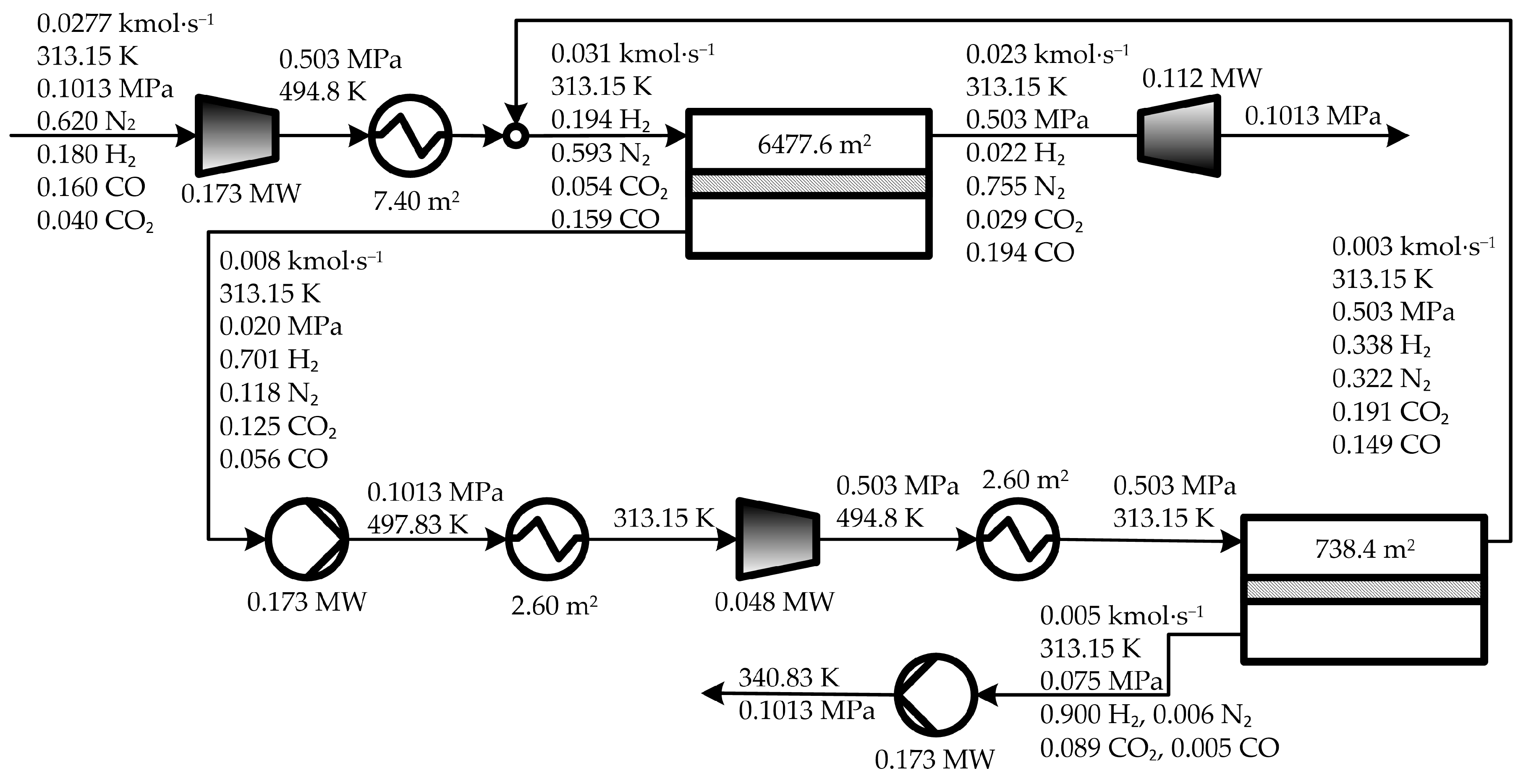
The comparison of results presented in Table 2 shows that the sub-optimal solution SUBOPT2 has the highest TAC value, which is 23.7% and 7.1% higher than those obtained in OPT and SUBOPT1, respectively. This is a confirmation that the expander was correctly removed (in terms of costs) from the optimal OPT and the sub-optimal SUBOPT1 solutions. In SUBOPT2, the percentage contributions of OPEX and annCAPEX to the TAC are 58.3% and 41.7%, respectively. The net electric power demand in SUBOPT2 is 45.2% and 61.2% lower than those in OPT and SUBOPT1, respectively, but the total membrane area in SUBOPT2 is 26.6% and 67.9% higher than those obtained in OPT and SUBOPT1, respectively. Then, the investment required by the expander for power recovery in SUBOPT2 (which represents 25% of the C_INV) is more important than the decrease of the cost for electric power i.e., in OPEX savings.

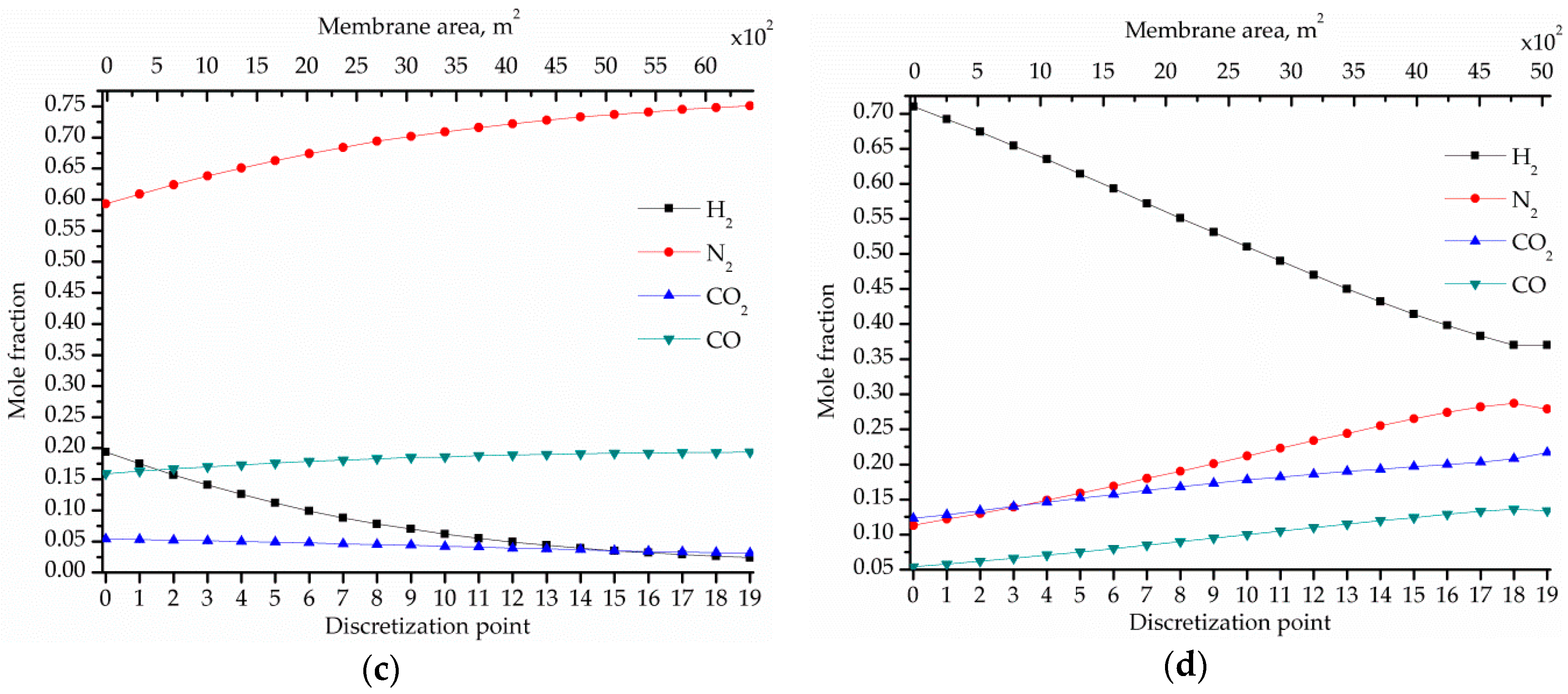
Also, it can be seen in Table 2 that the inclusion of the expander modifies the relevance order of the process-unit contributions to the total equipment acquisition investment C_INV, with the compressor C1 still being the largest contributor but now followed by the membrane area of the first stage, instead of the compressor C2 like in OPT and SUBOPT1. Figure 9 shows the component composition profiles in the retentate and permeate streams in the membrane modules MS1 and MS2 corresponding to SUBOPT2.

4.2. Sensitivity Analysis

This section presents a sensitivity analysis to see how the optimal solution discussed in the previous section is affected when the model parameters related to the design specifications i.e., H₂ product purity and H₂ recovery levels are varied one at the time by keeping constant the values of the remaining parameters.

4.2.1. Sensitivity of the Optimal Solution to the H₂ Product Purity Level

The optimization results obtained by varying the H₂ product purity in −0.01 (−1.11%) and +0.01 (+1.11%) with respect to the value used in the previous section (0.90) are compared in

Table 3. Sensitivity of the optimal solution to the H₂ product purity for a H₂ recovery of 90% and H₂ permeance of 2.871 × 10⁻² mole·m⁻²·s⁻¹·MPa⁻¹.

	H2 Product Purity
	Dev. (%)	0.89	0.90	0.91	Dev. (%)
Cost item
TAC (M$·year−1)	−1.32	1.741	1.764	1.802	+2.11
OPEX (M$·year−1)	−1.30	1.081	1.095	1.118	+2.04
annCAPEX (M$·year−1)	−1.36	0.660	0.669	0.684	+2.24
CINV (M$)	−1.36	1.411	1.431	1.463	+2.24
IC1	−1.24	0.685	0.694	0.705	+1.63
IC2	−4.72	0.302	0.316	0.337	+6.46
IMA_MS1	+1.48	0.273	0.269	0.266	−1.00
IVP1	−5.80	7.22 × 10−2	7.67 × 10−2	8.28 × 10−2	+8.04
IMA_MS2	+15.83	3.94 × 10−2	3.40 × 10−2	2.96 × 10−2	−12.88
IHEX1	−0.49	2.02 × 10−2	2.03 × 10−2	2.04 × 10−2	+0.54
IHEX2	−4.11	1.02 × 10−2	1.07 × 10−2	1.13 × 10−2	+5.79
IHEX3	−3.74	1.00 × 10−2	1.04 × 10−2	1.09 × 10−2	+4.99
CRM (M$·year−1)	−3.18	0.150	0.155	0.162	+4.52
CE	−3.67	0.136	0.141	0.148	+5.06
CMR	+3.07	1.175 × 10−2	1.140 × 10−2	1.113 × 10−2	−2.36
CCW	−4.30	2.67 × 10−3	2.79 × 10−3	2.95 × 10−3	+5.73
Design item
pH (MPa)	−2.84	0.581	0.598	0.621	+3.84
TMA (m2)	+3.10	5878.9	5701.7	5567.3	−2.35
TW (MW)	−3.69	0.287	0.298	0.313	+5.03

.

According to Table 3, the TAC value increases by 2.11% (from 1.764 M$·year⁻¹ to 1.802 M$·year⁻¹) when the H₂ product purity increases in 0.01 with respect to the reference case (0.90 H₂ purity). This increase is due to the increase of both the annCAPEX and OPEX values by 2.24% and 2.04%, respectively. It is interesting to note that, compared to the reference case, the electric power required by compressors and vacuum pump increases in total 0.015 MW while the optimal total membrane area decreases 134.4 m². The increased H₂ product purity level (0.91) implies to increase the H₂ concentration in the permeate stream of the first stage to reach the H₂ purity in the permeate stream of the second stage (the target level of 0.91). Then, the optimal cost-based trade-offs indicate that it is more beneficial to increase the total electrical power (from 0.598 MPa to 0.621 MPa) to operate the process at a higher operating pressure value p^H rather than to increase the total membrane area.

On the other hand, the TAC value decreases by 1.32% (from 1.764 M$·year⁻¹ to 1.741 M$·year⁻¹) when the H₂ product purity decreases in 0.01 with respect to the reference level. In this case, the annCAPEX and OPEX values decrease by 1.36% and 1.30%, respectively.

By comparing the percentage variation in Table 3, it can be concluded that the variations of TAC, annCAPEX, and OPEX are nonlinear. Also, it can be seen that the order of importance of the contributions of the process units is not influenced by the changes made on the H₂ product purity.

Finally, it is worth of mention that the (optimal) trends of the total electric power and membrane area are opposite, independently of the H₂ purity target level. This means that the higher the desired H₂ purity, the higher the demanded total electric power and the lower the required total membrane area; while the lower the H₂ purity, the lower the electric power and the higher the membrane area.

4.2.2. Sensitivity of the Optimal Solution to the H₂ Recovery Level

Table 4. Sensitivity of the optimal solution to the H₂ recovery level for a H₂ product purity of 0.90 and a H₂ permeance of 2.871 × 10⁻² mole·m⁻²·s⁻¹·MPa⁻¹.

			H2 Recovery
	Dev. (%)	89%	90%	91%	Dev. (%)
Cost Item
TAC (M$·year−1)	−1.49	1.738	1.764	1.793	+1.64
OPEX (M$·year−1)	−1.40	1.080	1.095	1.112	+1.54
annCAPEX (M$·year−1)	−1.64	0.658	0.669	0.681	+1.80
CINV (M$)	−1.64	1.407	1.431	1.457	+1.80
IC1	−1.34	0.684	0.694	0.703	+1.42
IC2	−3.22	0.306	0.316	0.328	+3.58
IMA_MS1	−0.88	0.266	0.268	0.271	+0.95
IVP1	−3.17	7.48 × 10−2	7.67 × 10−2	7.94 × 10−2	+3.57
IMA_MS2	+3.59	3.52 × 10−2	3.40 × 10−2	3.27 × 10−2	−3.76
IHEX1	−0.54	2.02 × 10−2	2.03 × 10−2	2.04 × 10−2	+0.44
IHEX2	−2.24	10.45 × 10−3	10.70 × 10−3	10.95 × 10−3	+2.43
IHEX3	−1.72	1.02 × 10−2	1.04 × 10−2	1.06 × 10−2	+1.82
CRM (M$·year−1)	−2.74	0.151	0.155	0.160	+3.02
CE	−2.92	0.137	0.141	0.145	+3.23
CMR	−0.35	1.136 × 10−2	1.140 × 10−2	1.145 × 10−2	+0.43
CCW	−2.86	2.71 × 10−3	2.79 × 10−3	2.88 × 10−3	+3.22
Design item
pH (MPa)	−3.01	0.580	0.598	0.618	+3.34
TMA (m2)	−0.36	5680.9	5701.7	5725.2	+0.41
TW (MW)	−3.02	0.289	0.298	0.307	+3.02

shows the influence of the H₂ recovery variation on the optimal solution. The minimum TAC value obtained for a H₂ recovery of 89% is 1.738 M$·year⁻¹, which represents a reduction of 1.49% with respect to the obtained for 90%. An increment in the H₂ recovery of 0.01 leads to an increase in the TAC of 0.029 M$·year⁻¹ which represents an increase of 1.64%.

Unlike the optimal trends observed for H₂ product purity variations, Table 4 shows that the requirements of electric power and membrane area follow the same behaviors, i.e., they both decrease with decreasing H₂ recovery levels, and vice versa. In addition, the variations of TAC, annCAPEX, and OPEX shown in Table 4 are not as nonlinear as those shown in Table 3.

The application of the here proposed model-based optimization approach has been successfully applied by the authors in other processes such as single-purpose seawater desalination plants [34,35,36], dual-purpose desalination plants [37,38], combined cycle power plants [39,40], amine-based CO₂ capture processes [41,42], biological wastewater treatment plants [43,44], real-time optimization in energy systems [45], liquid biofuel processors for H₂ production coupled to stationary fuel cells [46,47] and its associated heat exchanger network for optimal energy integration [48]. For instance, based on process models, this approach allowed to find a new cost-effective configuration for multi-stage flash desalination processes [35,36], which differ from the conventional configuration in the locations of distillate, recycle, and discharge streams. In combined cycle power plants [39,40], the simultaneous optimization approach allowed to find a new layout for the heat recovery steam generator (HRSG), which differs from the conventional configuration in the way in which heat exchangers (economizers, evaporators, and superheaters) are interconnected between them.

5. Conclusions

This paper presented the optimization results of two-stage membrane processes for H₂ separation from a multi-component gas mixture by applying nonlinear mathematical programming approach for cost minimization.

A set of nonlinear algebraic equations obtained by discretization of a set of nonlinear differential ordinary equations, applying backward finite difference method (BFDM), which describe gas permeation through a polymeric membrane in a counter-current flow pattern was implemented in GAMS.

Expanders, compressors, vacuum pumps, heat exchangers, splitters, mixers, and membrane modules were appropriately interconnected to represent different two-stage membrane process configurations (embedded configurations) to find the structure that determines the minimum total annual cost, while meeting target H₂ purity and H₂ recovery specifications in the product (permeate) stream.

Firstly, when the proposed optimization model was solved without imposing any structural constraints, no expander was selected and the driving force in the membrane stages was created by combining feed/permeate compression and retentate under vacuum (optimal solution OPT). For cost model and design specifications considered in this work, a minimum total annual cost of about 1.764 M$·year⁻¹ was obtained. Then, when constraints were imposed to prevent the use of vacuum in the permeate streams, the expander was again eliminated from the sub-optimal solution SUBOPT1, resulting in a total annual cost of about 2.038 M$·year⁻¹. This result clearly indicates that no benefit is obtained by including an expander to decrease the net electric power requirement. In other words, the investment required by the expander does not compensate the resulting decrease in the electric power requirement. This was confirmed by solving a third optimization problem, in which a constraint forcing the presence of the expander was considered. The total annual cost increased by about 24% with respect to that obtained in OPT (2.182 vs. 1.764 M$·year⁻¹) and 7% with respect to that obtained in SUBOPT1 (2.182 vs. 2.038 M$·year⁻¹).

The globality of the solutions here discussed cannot be guaranteed since a local search optimization algorithm is used.

The mathematical optimization model presented in this paper constitutes a valuable tool for simultaneously optimizing all trade-offs existing in a two-stage membrane process. It is also important to mention that the model can be easily extended to include additional membrane stages to embed more candidate configurations in order to have a model of multi-stage membrane-based processes for gas separations with more stringent product specifications.

The optimization of multi-stage membrane processes considering the possibility of using different membrane materials in each stage, as proposed in several applications [49,50,51,52,53] will be investigated, as well as hybrid systems that combine membrane-based processes with other technologies such as adsorption [54,55,56].

References

- Drioli, E.; Giorno, L.; Fontananova, E. Comprehensive Membrane Science and Engineering, 2nd ed.; Elsevier: Amsterdam, The Netherlands, 2017; ISBN 978-0-444-63796-3. [Google Scholar]
- Castel, C.; Favre, E. Membrane separations and energy efficiency. J. Membr. Sci. 2018, 548, 345–357. [Google Scholar] [CrossRef]
- Baker, R.W.; Low, B.T. Gas separation membrane materials: A perspective. Macromolecules 2014, 47, 6999–7013. [Google Scholar] [CrossRef]
- Sharif, A. Polymeric gas separation membranes: What makes them industrially more attractive? J. Membr. Sci. Res. 2018, 4, 2–3. [Google Scholar] [CrossRef]
- Ahmad, F.; Lau, K.K.; Lock, S.S.M.; Rafiq, S.; Khan, A.U.; Lee, M. Hollow fiber membrane model for gas separation: Process simulation, experimental validation and module characteristics study. J. Ind. Eng. Chem. 2015, 21, 1246–1257. [Google Scholar] [CrossRef]
- He, X.; Hägg, M.-B.; Kim, T.-J. Hybrid FSC membrane for CO2 removal from natural gas: Experimental, process simulation, and economic feasibility analysis. AIChE J. 2014, 60, 4174–4184. [Google Scholar] [CrossRef]
- Low, B.T.; Zhao, L.; Merkel, T.C.; Weber, M.; Stolten, D. A parametric study of the impact of membrane materials and process operating conditions on carbon capture from humidified flue gas. J. Membr. Sci. 2013, 431, 139–155. [Google Scholar] [CrossRef]
- Lin, H.; Zhou, M.; Ly, J.; Vu, J.; Wijmans, J.G.; Merkel, T.C.; Jin, J.; Haldeman, A.; Wagener, E.H.; Rue, D. Membrane-based oxygen-enriched combustion. Ind. Eng. Chem. Res. 2013, 52, 10820–10834. [Google Scholar] [CrossRef]
- Merkel, T.C.; Lin, H.; Wei, X.; Baker, R. Power plant post-combustion carbon dioxide capture: An opportunity for membranes. J. Membr. Sci. 2010, 359, 126–139. [Google Scholar] [CrossRef]
- Freeman, B.; Hao, P.; Baker, R.; Kniep, J.; Chen, E.; Ding, J.; Zhang, Y.; Rochelle, G.T. Hybrid Membrane-absorption CO2 Capture Process. Energy Procedia 2014, 63, 605–613. [Google Scholar] [CrossRef]
- Lin, H.; He, Z.; Sun, Z.; Kniep, J.; Ng, A.; Baker, R.W.; Merkel, T.C. CO2-selective membranes for hydrogen production and CO2 capture—Part II: Techno-economic analysis. J. Membr. Sci. 2015, 493, 794–806. [Google Scholar] [CrossRef]
- Masebinu, S.O.; Aboyade, A.O.; Muzenda, E. Parametric study of single and double stage membrane configuration in methane enrichment process. In Proceedings of the World Congress on Engineering and Computer Science, San Francisco, CA, USA, 22–24 October 2014; Volume 2, pp. 581–589. [Google Scholar]
- Bounaceur, R.; Berger, E.; Pfister, M.; Ramirez Santos, A.A.; Favre, E. Rigorous variable permeability modelling and process simulation for the design of polymeric membrane gas separation units: MEMSIC simulation tool. J. Membr. Sci. 2017, 523, 77–91. [Google Scholar] [CrossRef]
- Makaruk, A.; Harasek, M. Numerical algorithm for modelling multicomponent multipermeator systems. J. Membr. Sci. 2009, 344, 258–265. [Google Scholar] [CrossRef]
- Kundu, P.K.; Chakma, A.; Feng, X. Simulation of binary gas separation with asymmetric hollow fibre membranes and case studies of air separation. Can. J. Chem. Eng. 2012, 90, 1253–1268. [Google Scholar] [CrossRef]
- Gabrielli, P.; Gazzani, M.; Mazzotti, M. On the optimal design of membrane-based gas separation processes. J. Membr. Sci. 2017, 526, 118–130. [Google Scholar] [CrossRef]
- Zhai, H.; Rubin, E.S. Techno-economic assessment of polymer membrane systems for postcombustion carbon capture at coal-fired power plants. Environ. Sci. Technol. 2013, 47, 3006–3014. [Google Scholar] [CrossRef] [PubMed]
- He, X.; Fu, C.; Hägg, M.-B. Membrane system design and process feasibility analysis for CO2 capture from flue gas with a fixed-site-carrier membrane. Chem. Eng. J. 2015, 268, 1–9. [Google Scholar] [CrossRef]
- Khalilpour, R.; Abbas, A.; Lai, Z.; Pinnau, I. Analysis of hollow fibre membrane systems for multicomponent gas separation. Chem. Eng. Res. Des. 2013, 91, 332–347. [Google Scholar] [CrossRef]
- Arias, A.M.; Mussati, M.C.; Mores, P.L.; Scenna, N.J.; Caballero, J.A.; Mussati, S.F. Optimization of multi-stage membrane systems for CO2 capture from flue gas. Int. J. Greenh. Gas Control 2016, 53, 371–390. [Google Scholar] [CrossRef]
- Khalilpour, R.; Mumford, K.; Zhai, H.; Abbas, A.; Stevens, G.; Rubin, E.S. Membrane-based carbon capture from flue gas: A review. J. Clean. Prod. 2015, 103, 286–300. [Google Scholar] [CrossRef]
- Yuan, M.; Narakornpijit, K.; Haghpanah, R.; Wilcox, J. Consideration of a nitrogen-selective membrane for postcombustion carbon capture through process modeling and optimization. J. Membr. Sci. 2014, 465, 177–184. [Google Scholar] [CrossRef]
- Lee, S.; Binns, M.; Kim, J.-K. Automated process design and optimization of membrane-based CO2 capture for a coal-based power plant. J. Membr. Sci. 2018, 563, 820–834. [Google Scholar] [CrossRef]
- Didaskalou, C.; Kupai, J.; Cseri, L.; Barabas, J.; Vass, E.; Holtzl, T.; Szekely, G. Membrane-Grafted Asymmetric Organocatalyst for an Integrated Synthesis-Separation Platform. ACS Catal. 2018, 8, 7430–7438. [Google Scholar] [CrossRef]
- Valtcheva, I.B.; Marchetti, P.; Livingston, A.G. Crosslinked polybenzimidazole membranes for organic solvent nanofiltration (OSN): Analysis of crosslinking reaction mechanism and effects of reaction parameters. J. Membr. Sci. 2015, 493, 568–579. [Google Scholar] [CrossRef]
- Qi, R.; Henson, M.A. Membrane system design for multicomponent gas mixtures via mixed-integer nonlinear programming. Comput. Chem. Eng. 2000, 24, 2719–2737. [Google Scholar] [CrossRef] [Green Version]
- Scholz, M.; Alders, M.; Lohaus, T.; Wessling, M. Structural optimization of membrane-based biogas upgrading processes. J. Membr. Sci. 2015, 474, 1–10. [Google Scholar] [CrossRef]
- Kim, M.; Kim, S.; Kim, J. Optimization-based approach for design and integration of carbon dioxide separation processes using membrane technology. Energy Procedia 2017, 136, 336–341. [Google Scholar] [CrossRef]
- Uppaluri, R.V.S.; Linke, P.; Kokossis, A.C. Synthesis and optimization of gas permeation membrane networks. Ind. Eng. Chem. Res. 2004, 43, 4305–4322. [Google Scholar] [CrossRef]
- Zarca, G.; Urtiaga, A.; Biegler, L.T.; Ortiz, I. An optimization model for assessment of membrane-based post-combustion gas upcycling into hydrogen or syngas. J. Membr. Sci. 2018, 563, 83–92. [Google Scholar] [CrossRef]
- Brunetti, A.; Barbieri, G.; Drioli, E. New Metrics in Membrane Gas Separation. In Membrane Engineering for the Treatment of Gases; Drioli, E., Barbieri, G., Eds.; Royal Society of Chemistry: London, UK, 2011; Chapter 19; pp. 279–301. [Google Scholar]
- Abu-Zahra, M.R.M.; Niederer, J.P.M.; Feron, P.H.M.; Versteeg, G.F. CO2 capture from power plants: Part II. A parametric study of the economical performance based on mono-ethanolamine. Int. J. Greenh. Gas Control 2007, 1, 135–142. [Google Scholar] [CrossRef]
- Rao, A.B.; Rubin, E.S. A Technical, Economic, and Environmental Assessment of Amine-Based CO2 Capture Technology for Power Plant Greenhouse Gas Control. Environ. Sci. Technol. 2002, 36, 4467–4475. [Google Scholar] [CrossRef] [PubMed]
- Mussati, S.; Aguirre, P.; Scenna, N.J. Optimal MSF plant design. Desalination 2001, 138, 341–347. [Google Scholar] [CrossRef]
- Mussati, S.F.; Aguirre, P.A.; Scenna, N.J. Novel Configuration for a Multistage Flash-Mixer Desalination System. Ind. Eng. Chem. Res. 2003, 42, 4828–4839. [Google Scholar] [CrossRef]
- Mussati, S.F.; Aguirre, P.A.; Scenna, N.J. Improving the efficiency of the MSF once through (MSF-OT) and MSF-mixer (MSF-M) evaporators. Desalination 2004, 166, 141–151. [Google Scholar] [CrossRef]
- Mussati, S.F.; Aguirre, P.A.; Scenna, N.J. A rigorous, mixed-integer, nonlineal programming model (MINLP) for synthesis and optimal operation of cogeneration seawater desalination plants. Desalination 2004, 166, 339–345. [Google Scholar] [CrossRef]
- Mussati, S.; Aguirre, P.; Scenna, N. Dual-purpose desalination plants. Part II. Optimal configuration. Desalination 2003, 153, 185–189. [Google Scholar] [CrossRef]
- Manassaldi, J.I.; Arias, A.M.; Scenna, N.J.; Mussati, M.C.; Mussati, S.F. A discrete and continuous mathematical model for the optimal synthesis and design of dual pressure heat recovery steam generators coupled to two steam turbines. Energy 2016, 103, 807–823. [Google Scholar] [CrossRef]
- Manassaldi, J.I.; Mussati, S.F.; Scenna, N.J. Optimal synthesis and design of Heat Recovery Steam Generation (HRSG) via mathematical programming. Energy 2011, 36, 475–485. [Google Scholar] [CrossRef]
- Mores, P.; Rodríguez, N.; Scenna, N.; Mussati, S. CO2 capture in power plants: Minimization of the investment and operating cost of the post-combustion process using MEA aqueous solution. Int. J. Greenh. Gas Control 2012, 10, 148–163. [Google Scholar] [CrossRef]
- Mores, P.L.; Godoy, E.; Mussati, S.F.; Scenna, N.J. A NGCC power plant with a CO2 post-combustion capture option. Optimal economics for different generation/capture goals. Chem. Eng. Res. Des. 2014, 92, 1329–1353. [Google Scholar] [CrossRef]
- Alasino, N.; Mussati, M.C.; Scenna, N. Wastewater treatment plant synthesis and design. Ind. Eng. Chem. Res. 2007, 46, 7497–7512. [Google Scholar] [CrossRef]
- Alasino, N.; Mussati, M.C.; Scenna, N.J.; Aguirre, P. Wastewater treatment plant synthesis and design: Combined biological nitrogen and phosphorus removal. Ind. Eng. Chem. Res. 2010, 49, 8601–8612. [Google Scholar] [CrossRef]
- Serralunga, F.J.; Mussati, M.C.; Aguirre, P.A. Model Adaptation for real-time optimization in energy systems. Ind. Eng. Chem. Res. 2013, 52, 16795–16810. [Google Scholar] [CrossRef]
- Francesconi, J.A.; Mussati, M.C.; Mato, R.O.; Aguirre, P.A. Analysis of the energy efficiency of an integrated ethanol processor for PEM fuel cell systems. J. Power Sources 2007, 167, 151–161. [Google Scholar] [CrossRef]
- Oliva, D.G.; Francesconi, J.A.; Mussati, M.C.; Aguirre, P.A. Energy efficiency analysis of an integrated glycerin processor for PEM fuel cells: Comparison with an ethanol-based system. Int. J. Hydrogen Energy 2010, 35, 709–724. [Google Scholar] [CrossRef]
- Oliva, D.G.; Francesconi, J.A.; Mussati, M.C.; Aguirre, P.A. Modeling, synthesis and optimization of heat exchanger networks. Application to fuel processing systems for PEM fuel cells. Int. J. Hydrogen Energy 2011, 36, 9098–9114. [Google Scholar] [CrossRef]
- Hussain, A.; Farrukh, S.; Minhas, F.T. Two-Stage Membrane System for Post-combustion CO2 Capture Application. Energy Fuels 2015, 29, 6664–6669. [Google Scholar] [CrossRef]
- Fernández-Barquín, A.; Casado-Coterillo, C.; Irabien, Á. Separation of CO2-N2 gas mixtures: Membrane combination and temperature influence. Sep. Purif. Technol. 2017, 188, 197–205. [Google Scholar] [CrossRef]
- Sluijs, J.P.V.D.; Hendriks, C.A.; Blok, K. Feasibility of polymer membranes for carbon dioxide recovery from flue gases. Energy Convers. Manag. 1992, 33, 429–436. [Google Scholar] [CrossRef]
- Brinkmann, T.; Pohlmann, J.; Bram, M.; Zhao, L.; Tota, A.; Escalona, N.J.; de Graaff, M.; Stolten, D. Investigating the influence of the pressure distribution in a membrane module on the cascaded membrane system for post-combustion capture. Int. J. Greenh. Gas Control 2015, 39, 194–204. [Google Scholar] [CrossRef] [Green Version]
- Gerber, E. Production of Electric Power from Fossil Fuel with Almost Zero Air Pollution. International Patent Application No. PCT/US2014/000213 28 May 2015. [Google Scholar]
- Li, B.; He, G.; Jiang, X.; Dai, Y.; Ruan, X. Pressure swing adsorption/membrane hybrid processes for hydrogen purification with a high recovery. Front. Chem. Sci. Eng. 2016, 10, 255–264. [Google Scholar] [CrossRef]
- Didaskalou, C.; Buyuktiryaki, S.; Kecili, R.; Fonte, C.P.; Szekely, G. Valorisation of agricultural waste with an adsorption/nanofiltration hybrid process: From materials to sustainable process design. Green Chem. 2017, 19, 3116–3125. [Google Scholar] [CrossRef]
- Akinlabi, C.O.; Gerogiorgis, D.I.; Georgiadis, M.C.; Pistikopoulos, E.N. Modelling, design and optimisation of a hybrid PSA-membrane gas separation process. In Proceedings of the 17th European Symposium on Computer Aided Process Engineering, Bucharest, Romania, 27–30 May 2007; Volume 24, pp. 363–370. [Google Scholar]
Figure 1.
Schematic of the studied two-stage membrane process for H2 separation. (MS represents membrane units, C compressors, HEX heat exchangers, VP vacuum pumps, EXP expansion turbine (expander), SP splitters, M mixers. PMS represents the permeate stream in MS, RMS retentate stream in MS, RRMS (internal) retentante recycle in MS, RRMS2_MS1 (external) retentate recycle from MS2 to MS1, R## represents the fraction of R that is expanded in EXP and R# the fraction of R that is not expanded in EXP, and pH and pL indicate high and low pressure, respectively).
Figure 2.
Schematic representation and nomenclature: (a) whole process; (b) membrane modules. (F indicates flow rate, Q heat load, T temperature, p pressure, x composition in feed/retentate streams, y composition in permeate streams, W power, A area of membrane and area of heat exchanger. The subscript i represents a mixture component, subscript j a discretization point along the membrane length, and subscript 0 the fresh feed).
Figure 3.
Optimal process configuration obtained in solution (OPT), in which the driving force is created by combining compression and vacuum and no expander is included.
Figure 4.
Optimal cost distributions: (a) contributions of the total annualized capital expenditures (annCAPEX) and total operating expenditures (OPEX) to the total annual cost (TAC); (b) Equipment investment (CINV); (c) contributions of the electric power (EP) cost, membrane replacement (MR) cost, and cooling water (CW) cost to the total utility cost (CRM).
Figure 5.
Optimal mole fraction profiles of the components in the membrane modules obtained in solution OPT, in which the driving force for permeation is created by combining compression and vacuum and no expander is included for power recovery: (a) Permeate in MS1; (b) Permeate in MS2; (c) Retentate in MS1; (d) Retentate in MS2.
Figure 6.
Sub-optimal solution SUBOPT1, in which the driving force for permeation is created by compression of the feed and permeate streams only (no vacuum) and no expander is included.
Figure 7.
Optimal mole fraction profiles of the components in the membrane modules obtained in solution SUBOPT1, in which the driving force for permeation is created by compression of the feed and permeate streams only (no vacuum) and no expander is included: (a) permeate in MS1; (b) permeate in MS2; (c) retentate in MS1; (d) retentate in MS2.
Figure 8.
Sub-optimal solution SUBOPT2, in which the driving force for permeation is created by combining compression and vacuum and the expander is included for power recovery.
Figure 9.
Optimal mole fraction profiles of the components in the membrane modules obtained in solution SUBOPT2, in which the driving force for permeation is created by combining compression and vacuum and the expander is included for power recovery: (a) permeate in MS1; (b) permeate in MS2; (c) retentate in MS1; (d) retentate in MS2.