Local Fixed Pivot Quadrature Method of Moments for Solution of Population Balance Equation


1
School of Human Settlements and Civil Engineering, Xi’an Jiaotong University, Xi’an 710049, China
2
Key Laboratory of Ocean Energy Utilization and Energy Conservation of Ministry of Education, Dalian 116024, China
3
Mechanical Engineering College, Xi’an Shiyou University, Xi’an 710065, China
4
School of Aerospace, Xi’an Jiaotong University, Xi’an 710049, China
5
State Key Laboratory for Strength and Vibration of Mechanical Structures, Xi’an Jiaotong University, Xi’an 710049, China
*
Author to whom correspondence should be addressed.
Processes 2018, 6(11), 209; https://doi.org/10.3390/pr6110209
Submission received: 16 September 2018
/
Revised: 18 October 2018
/
Accepted: 25 October 2018
/
Published: 31 October 2018
(This article belongs to the Special Issue Recent Advances in Population Balance Modeling)
Abstract
:A local fixed pivot quadrature method of moments (LFPQMOM) is proposed for the solution of the population balance equation (PBE) for the aggregation and breakage process. First, the sectional representation for aggregation and breakage is presented. The continuous summation of the Dirac Delta function is adopted as the discrete form of the continuous particle size distribution in the local section as performed in short time Fourier transformation (STFT) and the moments in local sections are tracked successfully. Numerical simulation of benchmark test cases including aggregation, breakage, and aggregation breakage combined processes demonstrate that the new method could make good predictions for the moments along with particle size distribution without further assumption. The accuracy in the numerical results of the moments is comparable to or higher than the quadrature method of moment (QMOM) in most of the test cases. In theory, any number of moments can be tracked with the new method, but the computational expense can be relatively large due to many scalar equations that may be included.
1. Introduction
Determination of the interfacial area with high accuracy between different phases in a dispersed system is critical to the prediction of the flow behaviors and mass transfer. Population balance equation (PBE)—as an essential tool to describe the multiphase system and capable of predicting the interfacial area by tracking the particle size distribution and describing the micro-behaviors that influence the particle size distribution of the disperse phase—has been widely used in scientific and engineering fields. Unfortunately, such an equation is rather complex, and the numerical method is the only choice in most cases. Several predominate numerical methods have been proposed previously, which can be divided broadly into three categories: discretization methods (DM) [1,2,3,4,5,6], methods of moment (MOM) [7,8,9,10,11,12], and stochastic methods (SM) [13,14,15]. However, it is difficult for these methods to track both particle size distribution and its moments with high accuracy. In a recent paper, a promising numerical scheme—the sectional quadrature method of moment (SQMOM)—was proposed by Attarakih et al. for solving the PBEs for aggregation and breakage processes [16]. With the new scheme, both the particle size distribution and its moments could be tracked. However, several problems accompany these new methods. (1) In SQMOM, the semi-infinite solution domain [0, ∞) is truncated into a finite domain [Vmin, Vmax]. Using a finite domain to represent an infinite domain will inevitably introduce errors, which are referred to as finite domain errors. As a result, the moments cannot be tracked exactly. This is inherent in almost all DMs. In this sense, SQMOM is a kind of DM more than MOM. (2) If a new born particle with a volume smaller than Vmin or larger than Vmax is introduced by a certain event (aggregation or breakage), the event will be omitted. Therefore, the new method may influence the physical models in some extreme situations. (3) In SQMOM, the product-different (PD) algorithm [17] must be employed to obtain the abscissas and the weights in each section when a relatively large number of moments (≥6) need to be tracked. However, in PD, the values of abscissas are not restricted to the section they should belong to in mathematics. Hence, with the PD algorithm, the abscissas obtained might be outside the section they originally belong to. Until now, there is no effective solution to such a problem. Thus, it is almost impossible to track many moments with SQMOM.
In this work, the basic idea of STFT is applied to the aggregation and breakage processes, and a novel method, namely, the local fixed pivot quadrature method of moments (LFPQMOM) is proposed, with which moments can be tracked exactly. Meanwhile, the particle size distribution is constructed with high accuracy without introducing further assumption. This work is arranged as follows: a general form for population balance equation is presented, followed by the sectional representation for PBE including aggregation and breakage. Then, the local fixed pivot quadrature method of moments along with the treatment of the aggregation and breakage process is given. Finally, several benchmark test cases including pure aggregation, pure breakage, and aggregation and breakage combined processes are presented to validate the new method.
2. Population Balance Equation
Population balance equation is the continuous form of the number density function. In any disperse system, volume based PBE can be written as:
where f(V; x, t) is the number density function, describing the particle number distribution in property space referred to as internal coordinates, location, and time space referred as external coordinates, V is the particle volume, x is space location, t is time, and <ui>V is the particle velocity in the ith direction conditioned on volume V. S(V; t) describes the micro-behaviors of the particle swarm. In this work, we focus our attention on the solution method for the population balance equation for tracking particle size distribution and its moment due to aggregation and breakage at a given location x. To shorten the symbolic expression, space coordinate x is neglected in the discussion below.
A general description of aggregation in any particle system can be expressed as Equation (2), but with a different aggregation kernel.
where β(V, υ) is the aggregation kernel, the first term on the right hand side is the rate of birth of the particles with volume V due to aggregation of smaller particles, whereas the second is the rate of death of the particles with volume V due to their aggregation with other particles. The general description for breakage in any particle system can be expressed as follows, but with different breakage kernel or daughter distribution.
where a(V) is the breakage kernel and b(V| υ) is the daughter distribution. The first term on the right-hand side is the rate of birth of particles with volume V due to the breakup of larger particles, whereas the second is the rate of death of particles with volume V due to their breakup.
2.1. Sectional Representation for Population Balance Equation
Multiplying Equation (1) by a property function ψ(V) and integrating it over arbitrary domain [a, b] yields
Equation (4) is similar to, but not a weak form of, the solution of a general differential equation. A weak form is usually used to construct the algebraic relation of the original variable (particle size distribution f(V;t) in this work) through the integration relation of a differential equation over a cell (a section in this work). However, Equation (4) is used to construct the equations for the moments, which generally represent a physical quantity (total particle number, total particle volume, for instance)
Let the following relation be:
where m(t) can be regarded as the local moments of the number density function over the domain of [a, b]. ψ(V) is the property function, and, in the traditional moment methods, monomials are usually adopted. After some simple manipulations, Equation (4) can be written as:
where <ui> is the average velocity. The term on the right-hand side is the moment transformation for the micro-behaviors, aggregation, and breakage, for instance, influencing the evolution of m(x, t) in state space. Before deriving the actual expression of the source term, we introduce a switch function with a Boolean parameter.
2.2. Aggregation
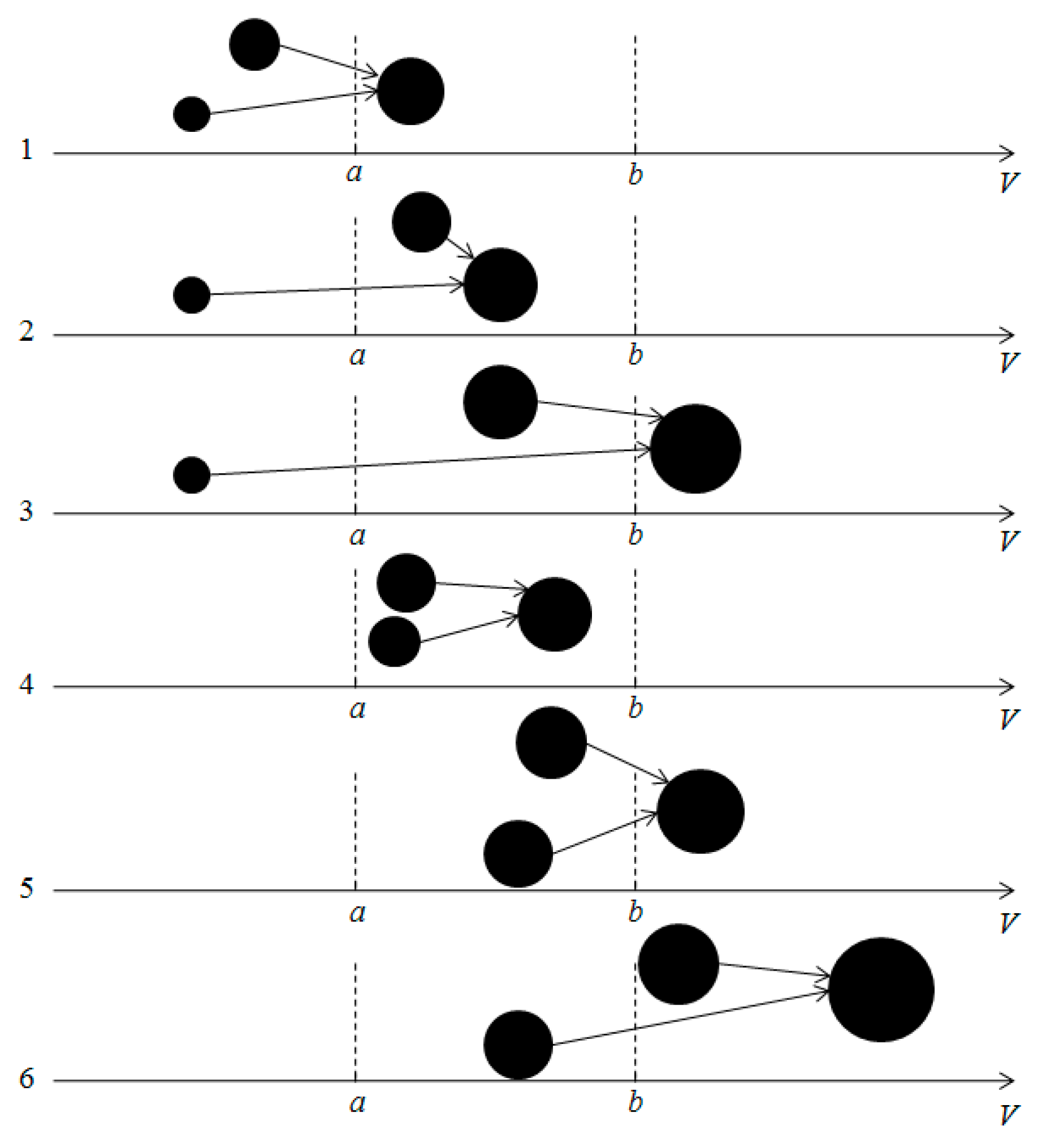
Here, we want to derive a general conservation equation for m(t). The contribution to the variation of the property m(t) in domain [a, b], due to aggregation, can be divided into six parts, as illustrated in Figure 1. In the figure, three kinds of particles can be made: A, particles with volume smaller than a; B, particles with volume between a and b; and C, particles with volume larger than b.
1. A + A → B: Particles with volumes lower than a aggregate to form particles with volume in [a, b). The net rate for the variation in m(t) due to this contribution is given by:
2. A + B → B: Particles with volume lower than a aggregate with particles with volume in [a, b) to form particles smaller than b. This contribution is given by:
3. A + B → C: Particles with volume lower than a aggregate with particles with volume in [a, b) to form particles larger than b. This will cause a net loss for m(t) which can be written:
4. B + B → B: Particles with volume in [a, b) aggregate to form particles in the same range. This contribution can be written as:
5. B + B → C: Particles with volume in [a, b) aggregate to form particles larger than b and this contribution is given by:
6. B + C → C: Particles from the domain [a, b) aggregate with particles larger than b to form particles larger than b, which causes a net loss for m(t) in [a, b), and can be written as:
The net rate for the variation in m(t) over the domain [a, b) due to aggregation is the summation of Equations (8)–(13).
2.3. Breakage
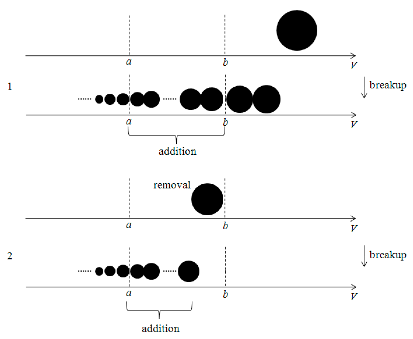
For the breakage process, the contribution to the change in m(t) over [a, b) can be divided into two parts, as illustrated in Figure 2. The particle classification is the same as that for aggregation process.
1. C → A + B + C: Particles with volume larger than b break up to form the particles in the domain [a, b). This contribution is given by:
2. B → B + C: Particles in the domain [a, b) break up to form the particles in the same range. This part can be written as:
The first term on the right-hand side is the removal of particles due to the particle breakage in [a, b) and the second is the addition of particle properties due to the particle birth.
The total contribution to the variation of m(t) due to the particle breakage is the summation of Equations (14) and (15).
3. Local Fixed Pivot Quadrature Method of Moments
To track the moments exactly in this work, the particle size distribution was assumed to have the form.
where ωi(t) are the weights; Vi are the quadrature nodes (pivots); n is the number of the quadrature nodes; and δ(V) is the Dirac Delta function.
It should be noted that Fourier transform of the Dirac Delta function is a constant of unity. The Dirac Delta functions in Equation (16) overlap one another in frequency space. Any changes in particle size distribution would be smoothed out; hence, it would not be possible to obtain the particle size distribution if Equation (16) is applied to the whole solution domain. As a result, we could not get the particle size distribution with traditional moment methods such as QMOM or FPQMOM. To retain information of particle size distribution, Equation (16) should be employed in the local domain as performed in short-time Fourier transformation (STFT).
To apply the idea of STFT to the new method, the volume space was divided into [0, υ1), [υ1, υ2), …, [υi, υi+1), …, [υN−1, ∞), N sections. Note that the section in the present work was equivalent to the cell (or bin) in the discretization methods and resembled the window in STFT. υi are the abscissas of the section ends, i.e., nodes. In this work, monomials were adopted as property function, i.e., ψ(V) = Vk (k = 0, 1, 2, …, n − 1). In the ith section, the moment equation (Equation (5)) becomes
Introducing Equation (16) into the ith section yields
where is the kth moment of section i; are the weights of the pivots in section i; is the jth pivot in section i and has to be specified beforehand; and ni is the number of the pivots in section i.
Equation (18) could be written in matrix form if k = 0, …, ni − 1 are adopted
Equation (19) is a vandermonde linear system, the coefficient matrix of which is rather ill-conditioned. Direct inversion of such a coefficient matrix or solving it using traditional numerical methods would inevitably introduce errors. We must resort to the special algorithm for such an equation set, and one such algorithm was recommended by Golub [18].
In theory, the locations of pivots in section i can be specified arbitrarily within [υi, υi+1) as long as each location has a unique value. It is worth pointing out that the main concern here is the numerical accuracy of the quadrature over [υi, υi+1) or [υn−1, ∞). It is well known that numerical integration of arbitrary smooth functions over a bounded interval is most accurate when carried out with quadrature points chosen as zeros of orthogonal polynomials. Several classical orthogonal polynomials are available [19] such as Gauss-Legendre over (−1, 1) with weighted function W(x) = 1, Gauss-Chebyshev over (−1, 1) with weighted function W(x) = (1 − x2)−1/2, Gauss-Laguerre over (0, ∞) with weighted function W(x) = xα e−x (α > −1), and Gauss-Jacobi over (−1, 1) with weighted function (1 − x)α(1 + x)β. The parameters, α in Gauss-Laguerre and α and β in Gauss-Jacobi, controlling the actual form of the polynomials can be used to optimize the distribution of the particle ensembles according to the actual distribution. Note that the orthogonal domains of Gauss-Legendre, Gauss-Chebyshev, and Gauss-Jocobi are not [υi, υi+1). Thus, a transformation is required before these polynomials can be used in the simulation. The following relation can serve this purpose if υi+1 ≠ ∞
Equation (20) is used to transform the pivots t in [−1, 1] to s in [υi, υi+1). The zeros of the orthogonal polynomial of Gauss-Laguerre with α = 0, are taken as the locations of pivots after transforming t in [0, ∞) to s in [υN−1, ∞) using a simple linear relation s = t + υN−1.
After transformation using this method, the Gauss-Chebyshev orthogonal polynomial is applied to the first n − 1 sections and Gauss-Laguerre to the last section. An exponential form is adopted when discretizing the property domain, i.e.,
with υ0 = 0 and υN = ∞. s is the scale factor.
3.1. Aggregation
For pure aggregation process, there are six terms (Equations (8)–(13)) to contribute the variation for the moments mk in each section. In this work, monomials were adopted as the property functions, i.e., ψ(V) = Vk (k = 0, 1, 2, …, n − 1). In the lth (l = 0, 1, …, N − 1) section, after introducing the approximation of Equation (16) and some manipulations, Equation (8) yields
Equation (9) yields
Equation (10) yields
Equation (11) yields
Equation (12) yields
and Equation (13) yields
where N is the total number of the sections; ni is the count of the pivots in section i; uij are the abscissas of jth pivot in section i; and ωij is the weight of jth pivot in section i.
The summation of Equations (22)–(27) can be abbreviated
3.2. Breakage
Two terms contribute the variation of the moments mk(t) in the pure breakage process. In the lth (l = 0, 1, …, N − 1) section, after introducing the approximation of Equation (16) and some manipulations, Equation (14) yields
and Equation (15) yields
The total contribution to the variation of mk(t) due to the breakage of particles is the summation of Equations (29) and (30).
3.3. Reconstruction of the Moments
In the new method, the moments in the local domain (section) are tracked. The moments of the particle size distribution are the summation of the moments in all the sections, i.e.,
3.4. Reconstruction of the Particle Size Distribution
The average particle number density in the ith section can be written as
The average particle size is defined as the weighted average of particles in section i
It is worth pointing out that, in traditional methods of moment (MOMs) such as quadrature method of moment (QMOM) [7] or fixed pivot quadrature method of moment (FPQMOM) [12], the assumption of continuous summation of the Dirac Delta function is adopted in the overall domain, thus the particle size distribution is lost in the simulation. With traditional MOMs, particle size distribution cannot be obtained. However, with the new method detailed here, the assumption of the continuous summation of the Dirac Delta function is adopted in the subsection, detailed information in the local domain is retained in the simulation, and, with this information, the particle size distribution can be reconstructed without any additional assumption. If only one section is adopted in the simulation, the method here is the same as FPQMOM.
4. Test Cases
In all test cases presented here, the volume space was divided into 40 sections using Equation (21) with υ1 = 0.01 and s = 1.2. In each section the six pivots were specified (i.e., six moments were tracked). A time step of 0.01 s was adopted. All simulations in this work were carried out on a desktop computer with Intel Core i5 CPU (3.1 GHz) and 8 G memory.
4.1. Pure Aggregation
Five test cases were carried out to validate the new method for the pure aggregation process, in the first of which a constant aggregation kernel was adopted, having the form
with C0 = 1, together with exponential initial particle size distribution
with N0 = 1, V0 = 1. In this test case, an analytical solution was available [20]
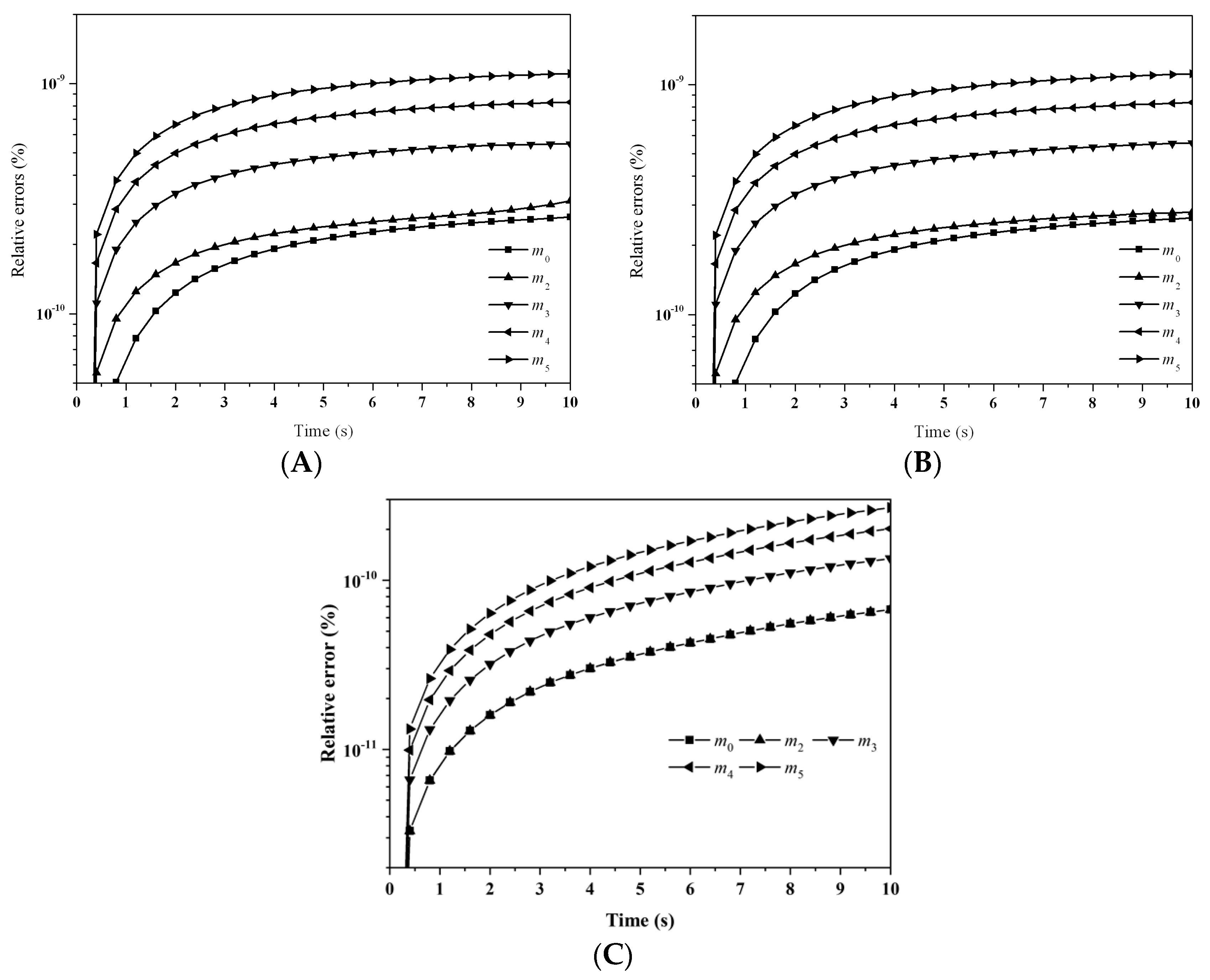
with T = C0N0t/(2 + C0N0t). The moments could be evaluated analytically. Figure 3 depicts the evolution of the percentage errors for the first six moments with: (A) LFPQMOM; (B) QMOM; and (C) FPQMOM. In the figure, the evolution for the relative errors for all the moments were similar in both methods, but a little larger than FPQMOM. Errors increased rapidly initially and leveled off after 2 s. The maximum percentage error with QMOM was 1.12 × 10⁻⁹%, whereas with the new method, it was 1.10 × 10⁻⁹%, a small decrease. FPQMOM had the highest accuracy. Higher rank moments had larger percentage errors with both methods. It is worth pointing out that, with LFPQMOM, the relative errors for m1 were always zero within the simulation time, but with QMOM, they were lower than 10−12%, but larger than zero. With the new method, m1 could be predicted without any error. In the figure, percentage errors for m1 were not included due to their low values.
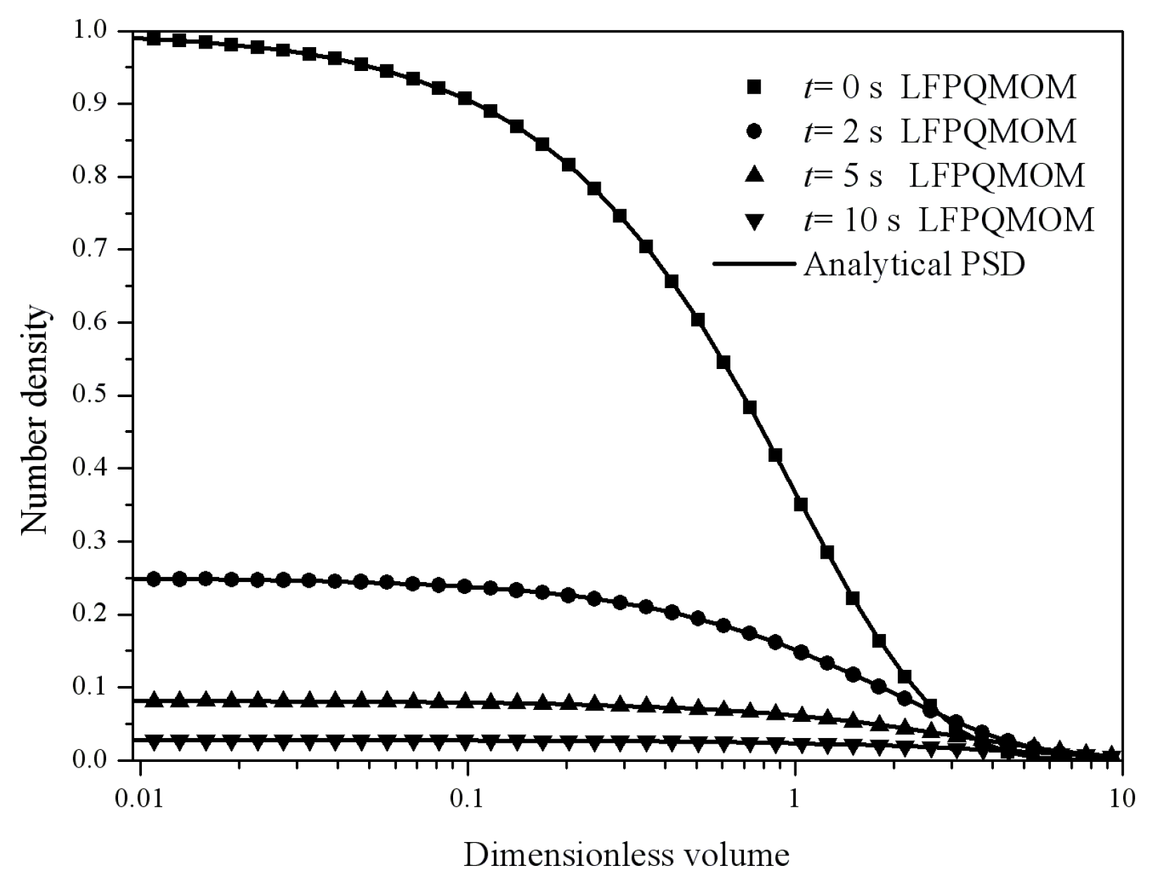
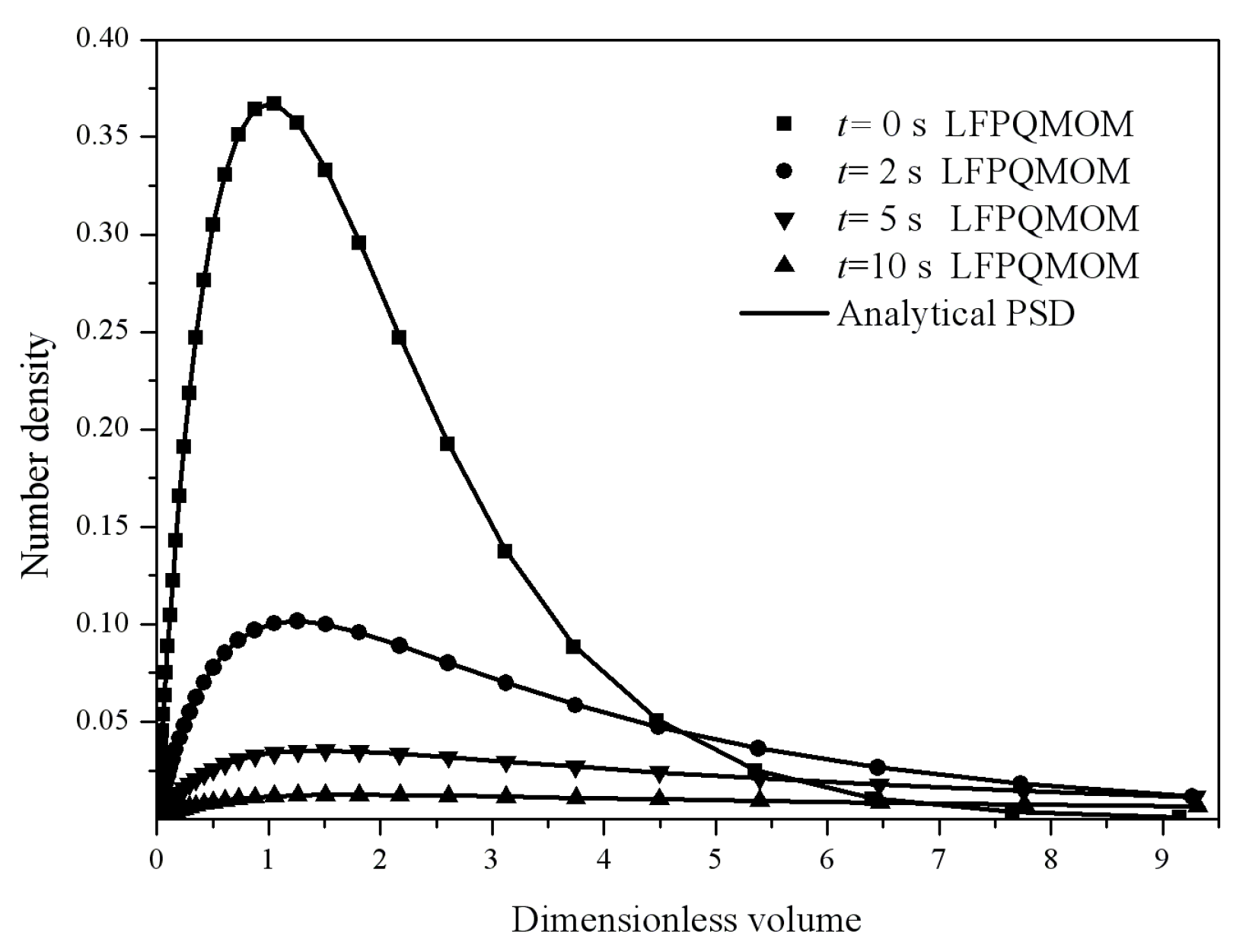
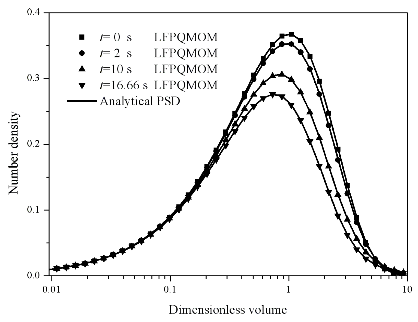
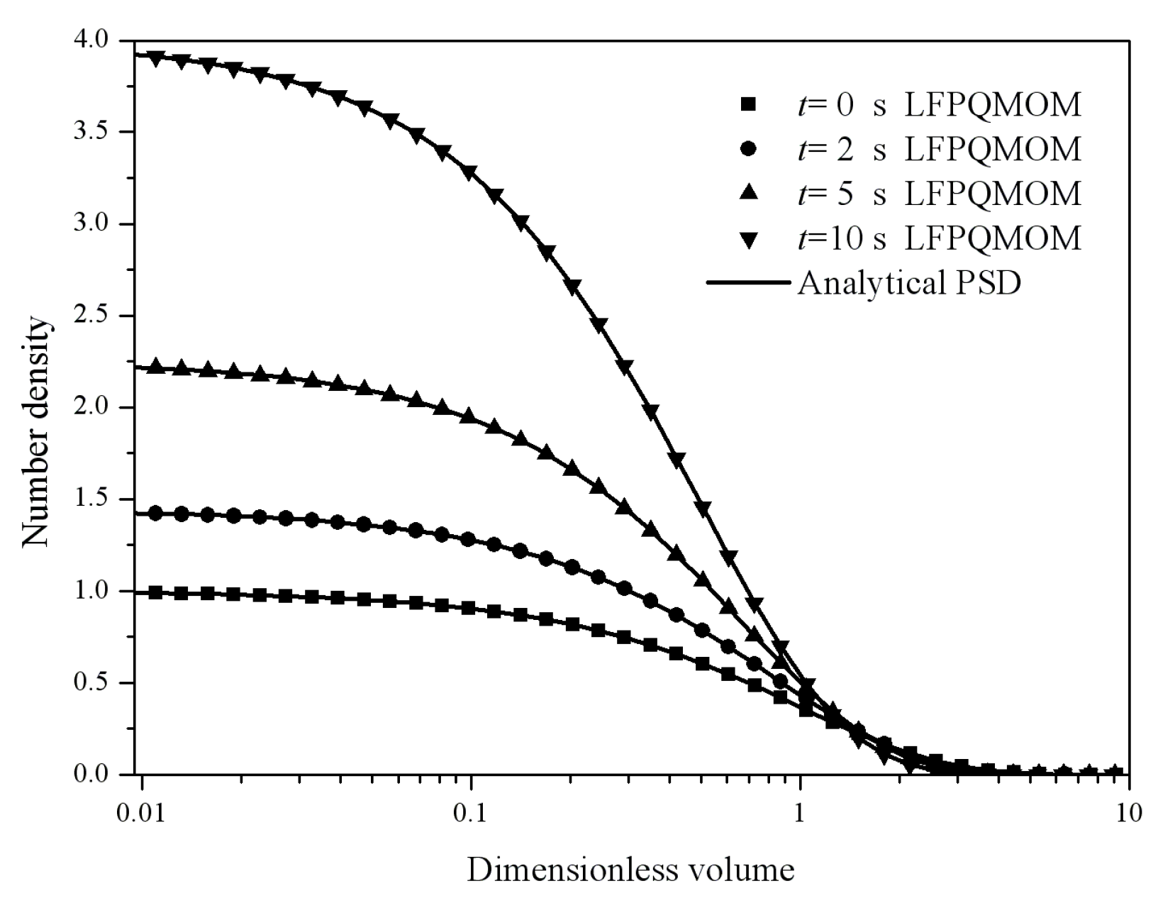
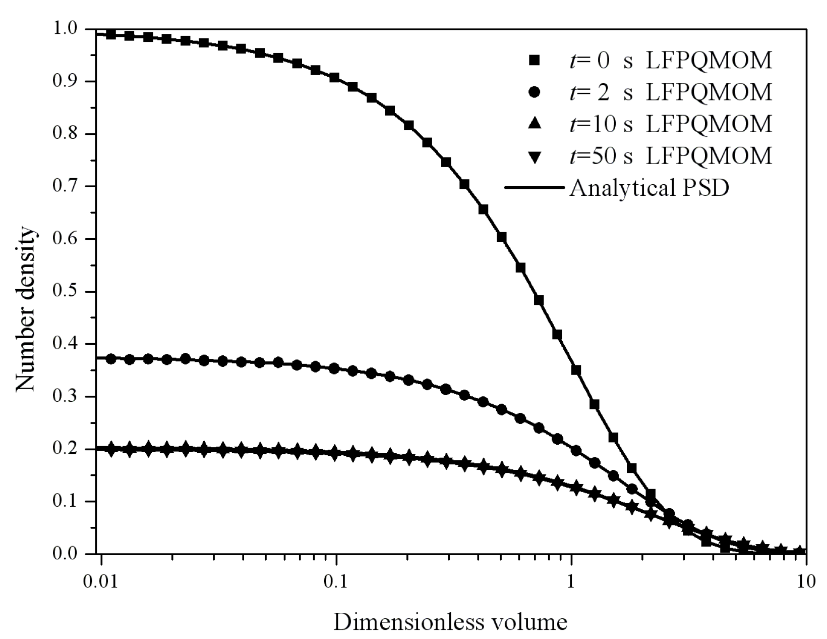
Figure 4 gives the particle size distribution predicted by LFPQMOM at 0, 2, 5, and 10 s. In the figure, the numerical PSDs agreed exactly with the analytical PSDs. The number density approached zero when the dimensionless volume was larger than 10.
The computational time was about 28,360, 1795, and 625 ms for LFPQMOM, QMOM, and FPQMOM, respectively. The computational load of LFPQMOM was much larger than QMOM and FPQMOM, since, in LFPQMOM, 40 sections were adopted in this work and, in each section, six moments were tracked. The total number of variables included in the simulation with LFPQMOM was 240, whereas, in QMOM and FPQMOM, only six variables were included. The computational time for each variable on average was 118, 299, and 104 ms for LFPQMOM, QMOM, and FPQMOM, respectively. From the view of a one-variable computational load, LFPQMOM and FPQMOM were more efficient than QMOM because of the vandermode linear system solver used.
In the second test case, a constant aggregation kernel was used, i.e., Equation (35) with C0 = 1, but with Gaussian initial particle size distribution, having the form
with N0 = 1 and V0 = 1. In this test case, analytical particle size distribution is given by [20]
with T = C0N0t/(2 + C0N0t). The moments can be evaluated analytically.
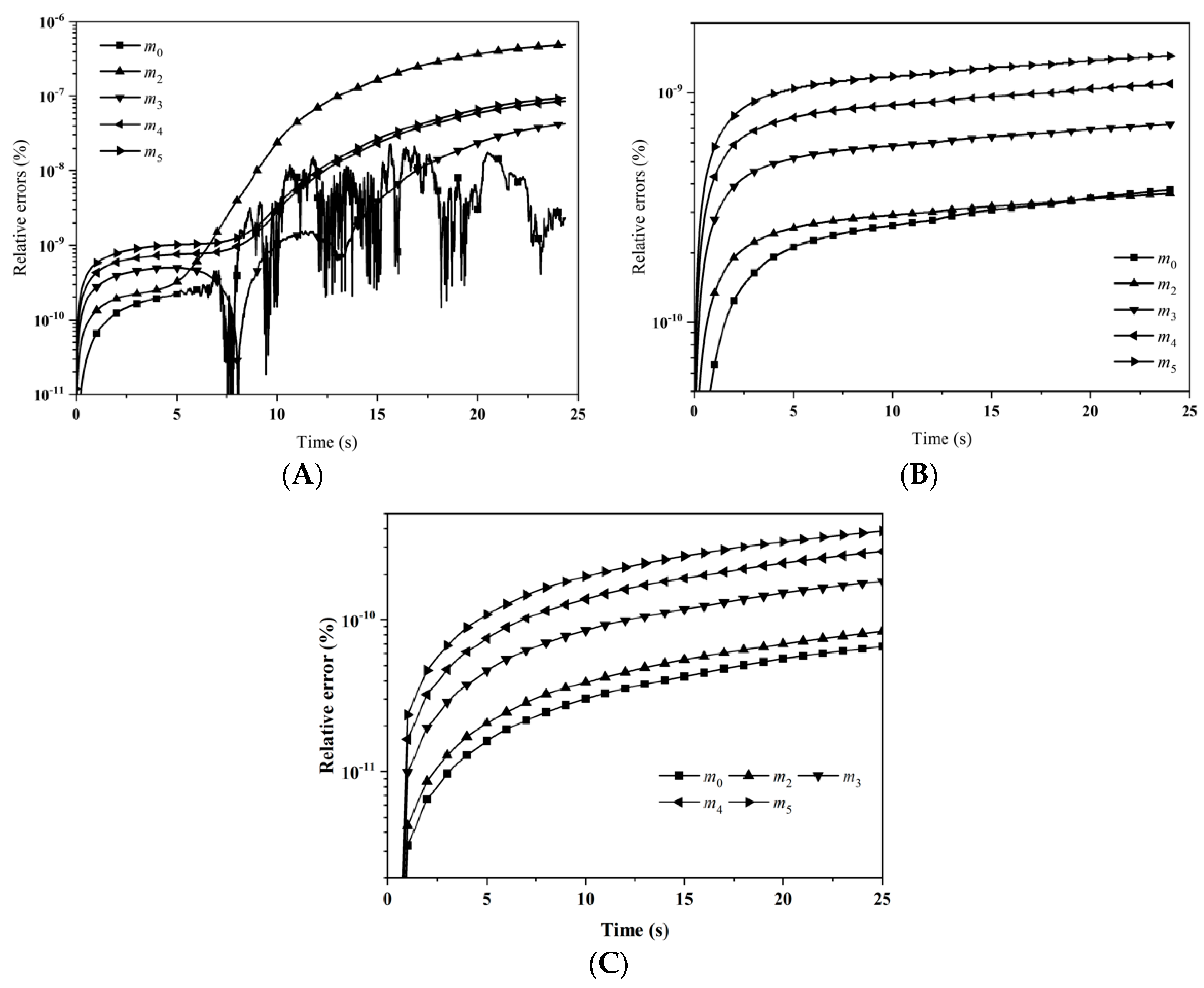
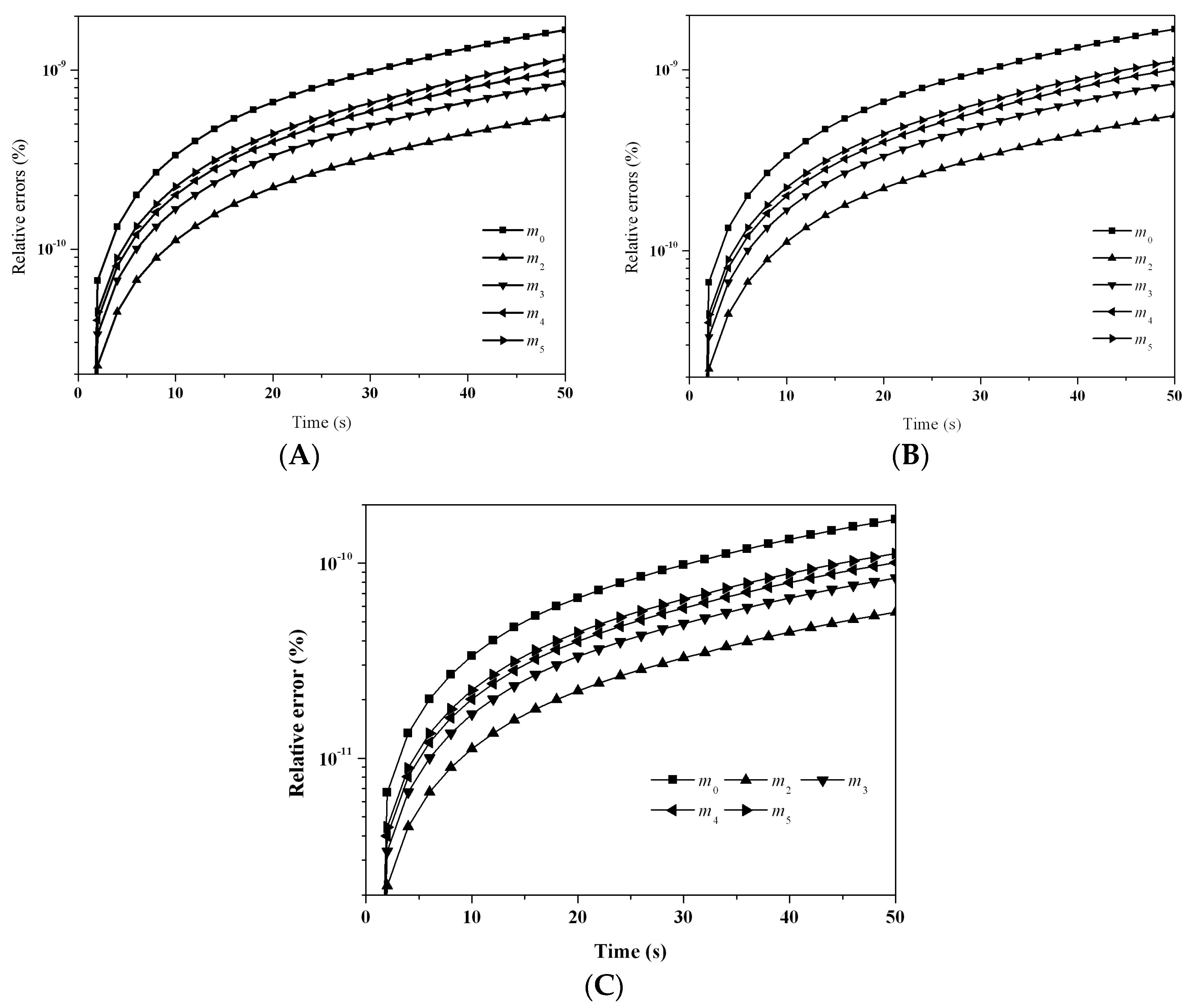
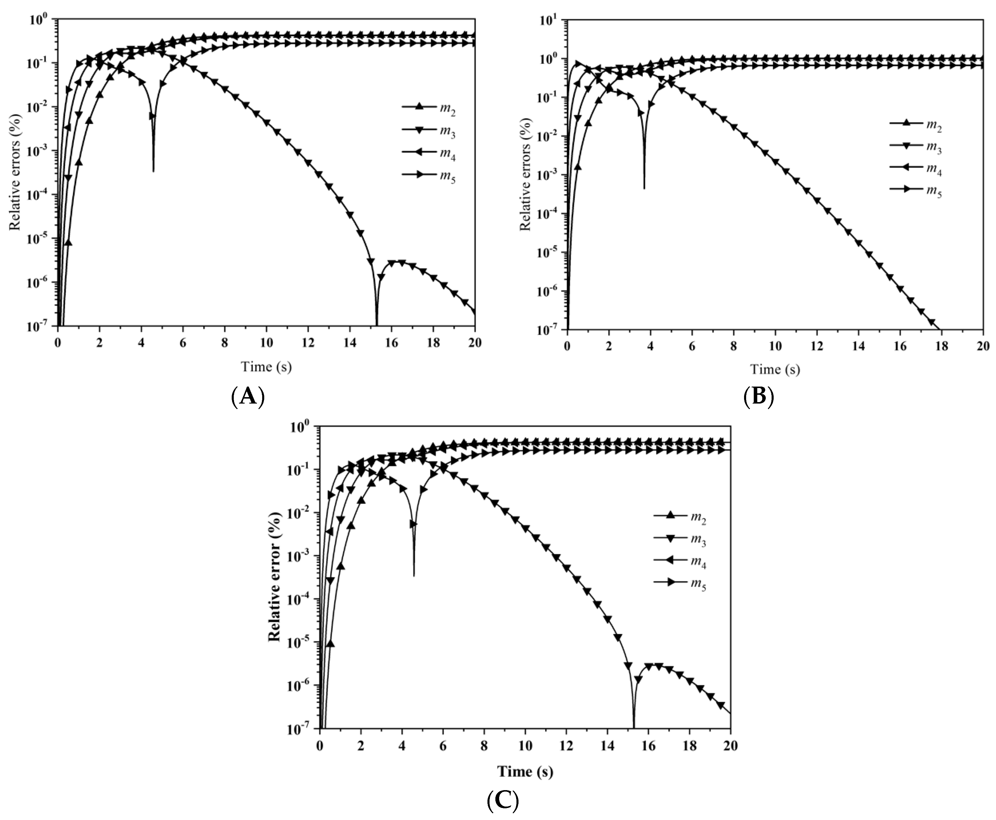
Figure 5 illustrates the relative errors for the first six moments with: (A) LFPQMOM; (B) QMOM; and (C) FPQMOM. With LFPQMOM, the relative errors rose rapidly initially, and became flat after 2 s. The relative errors for m2 after 6 s and m4 and m5 after 9 s began to rise, but for m0 and m3 they began to fluctuate after 7 s. With QMOM, the relative errors for all the moments rose sharply initially, and leveled off after 2 s, the evolution of which was very similar to that in the previous case. With the new method, the prediction for the moments of m2, m4, and m5 was poor relative to QMOM, but was lower 10−6% within the simulation time, which could still satisfy industrial needs. With FPQMOM, the numerical prediction was the best. In this test case, m3 could be predicted exactly without any error within the simulation time with the new method. The percentage errors for m3 were not included in the figure due to their low values with both methods. Figure 6 gives the particle size distribution predicted by LFPQMOM at 0, 2, 5, and 10 s, along with analytical solutions for comparison. In the figure, the numerical PSDs with our new method agreed well with the analytical PSDs. Again, the new method made an excellent prediction for both moments and PSD. The computational time was about 71,766, 5024, and 1709 for LFPQMOM, QMOM, and FPQMOM, respectively, in this test.
One should note that, with LFPQMOM, we did not track the moments of the PSD over the whole domain, but the moments in each section. As a result, to compute relative error with LFPQMOM, we had to resort to Equation (32) to first compute the moments of the PSD. Thus, the numerical errors of each moment presented in the figure for LFPQMOM are the compound errors, but not for one variable. For instance, to calculate errors of m3, we calculated the m3 with m3i of the whole PSD using Equation (32) first, and then compared it with its analytical counterpart where m3i is the tracked variable not m3. In each section, a fixed pivot quadrature method of moment (FPQMOM) was used. FPQMOM was more accurate than QMOM, as can be seen in the figure. As a result, the relative errors of the moments with FPQMOM do not deviate from QMOM or LFPQMOM too much. If the relative error for a tracked variable is too small, the values of the relative errors can be random. The compound relative errors can also be random. The fluctuations in the errors of m0 in Figure 5A may be related to this.
In the third test case, a sum aggregation kernel was used
with C0 = 0.01, together with the exponential initial distribution, i.e., Equation (36) with N0 = 1 and V0 = 1. Analytical solution was given by [20]
with x = V/V0 and τ = 1 − exp(−C0N0V0t). I1(x) is the modified Bessel function of the first kind. Moments can be evaluated using the numerical integration method.
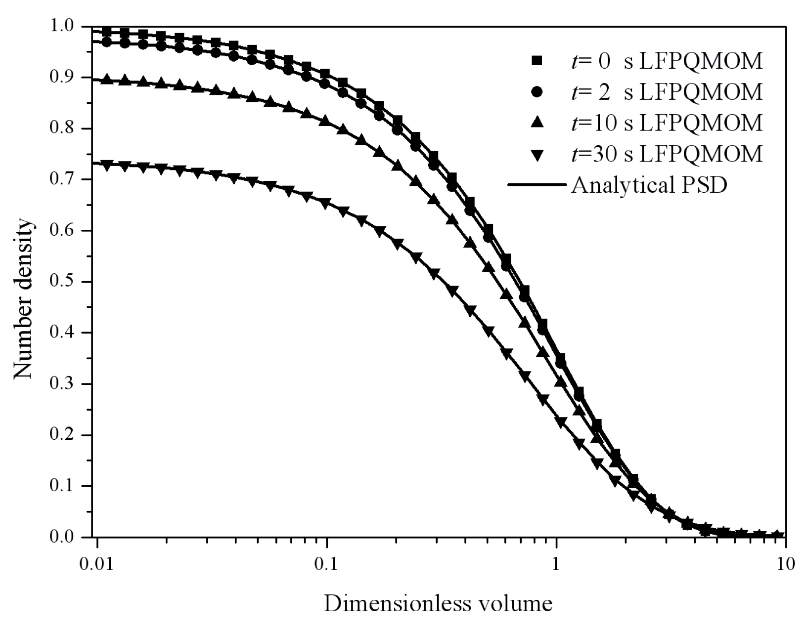
Figure 7 shows the evolution of percentage errors for the first six moments with: (A) LFPQMOM; (B) QMOM; and (C) FPQMOM. In the figure, within the simulation time, the relative errors for all the moments were lower than 10−5%. It should be noted that the relative errors for m1 were not lower than 10−12%, even though the conservation of the mass was considered in the new method. This is because no analytical solutions for the moments were available. The numerical errors for m1 were not caused by the new method or QMOM, but came from the evaluation of the moments through numerical integration. The sharp drops in the relative errors were related with the numerical errors of the evaluation of the moments. Figure 8 illustrates the particle size distribution at 0, 2, 10, and 30 s. It can be observed that the numerical predictions with the new method were in excellent agreement with the analytical counterparts. Number density with dimensionless volume larger than 10 approached zero. The computational time was about 86,314, 5570, and 1948 ms for LFPQMOM, QMOM, and FPQMOM, respectively.
In the fourth test case, a product aggregation kernel was adopted, having the form
with C0 = 0.01, together with the exponential initial PSD, i.e., Equation (36) with N0 = 1 and V0 = 1. Analytical solution for this test case was given by [20]
where , x = V/V0 and Γ (x) is the gamma function.
Note that the product kernel is a gelling kernel, and the second and higher moments will become infinite within finite time [21]. Most existing moment methods cannot predict the moments exactly, especially near the gelling point. The analytical solutions for moments m0, m1, and m2 are given in Table 1. Based on the solution for m2, the actual value for tgel can be calculated
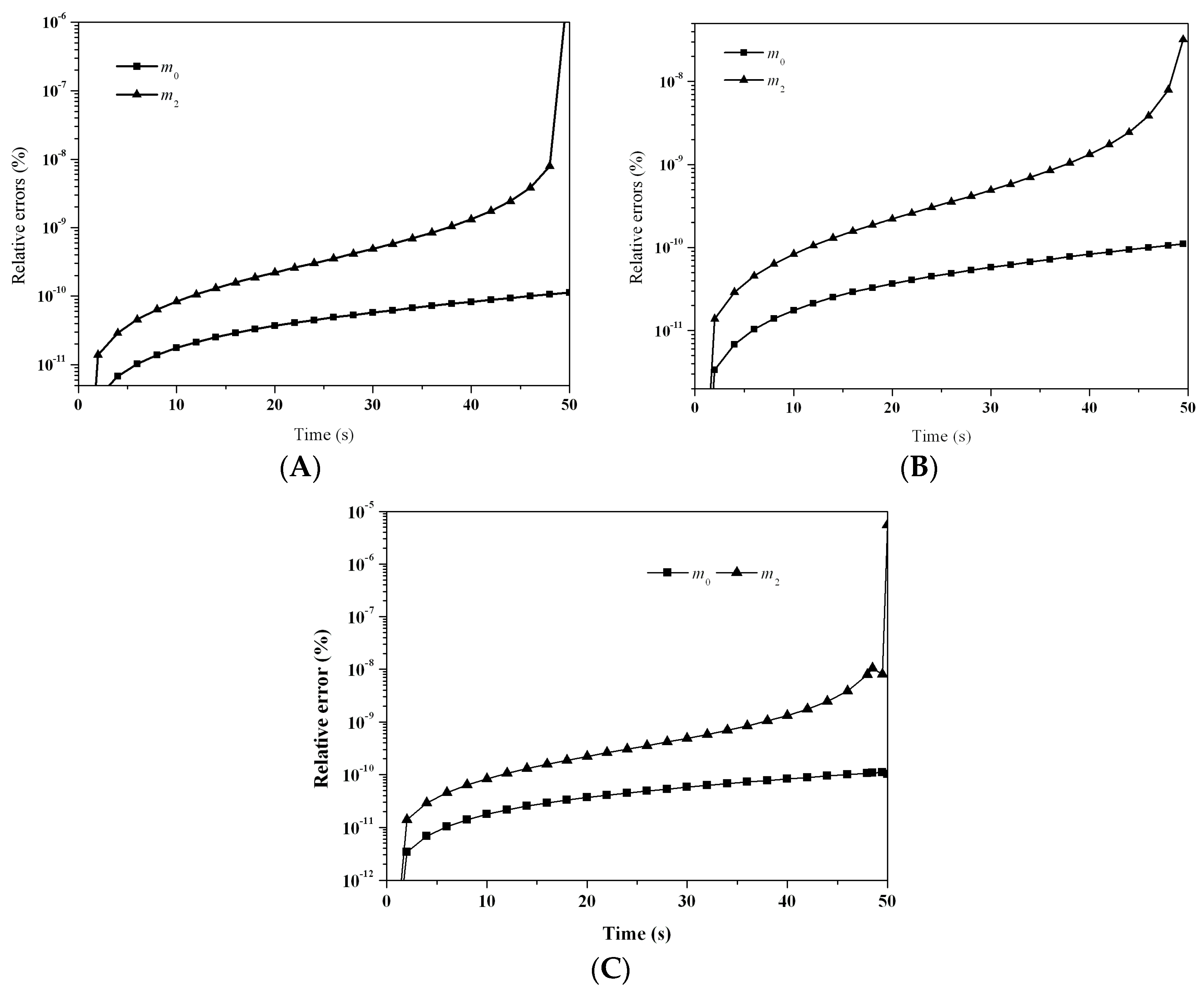
The gelling time tgel is 50 s in this test case. To predict the moments as exactly as possible, especially near the gelling point, two nodes were adopted for QMOM and three pivots in each section for LFPQMOM. The percentage errors of the first three moments are shown in Figure 9A–C for LFPQMOM, QMOM, and FPQMOM, respectively. An interesting feature with the new method is that the simulation can be carried out for as long as possible before the gelling point. The maximum time that can be used as the simulation time is tgel − Δt. Δt is the time step. In this test case, a time step of 0.01 s was adopted, thus any time of t ≤ 49.99 s could be adopted as the simulation time. With QMOM, only an even number of moments could be tracked, four moments in this test case. We could only carry out the simulation before the time of 49.6 s when m3 diverged. After that time, QMOM was not appropriate, and the new method could also make a good prediction, with a relative error smaller than 10−5%, as can be seen in Figure 9A. Relative errors with FPQMOM were similar to those with LFPQMOM. The relative errors for m1 with all methods here were lower than 10−13%, hence were not included in the figures. Figure 10 shows a good agreement of numerical PSD predicted by the new method at 0, 10, 20, and 50 s with the analytical solution. Number density approached zero with a dimensionless volume larger than 10. The computational time was about 143,962, 8957, and 3199 ms for LFPQMOM, QMOM, and FPQMOM, respectively, in this test.
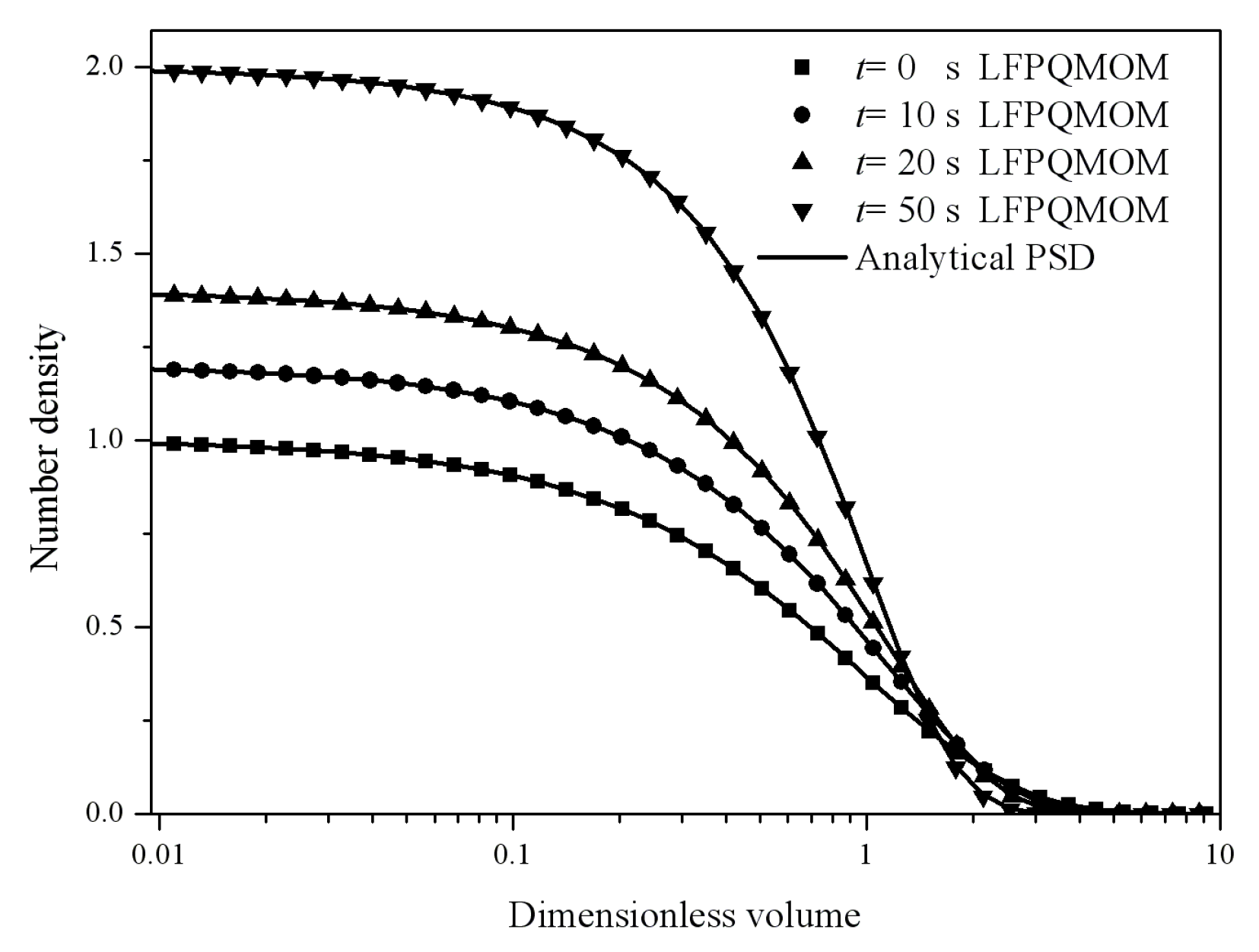
In the final test case for pure aggregation, a product kernel was used, i.e., Equation (42) with C0 = 0.01, but with a Gaussian initial PSD, i.e., Equation (38) with N0 = 1 and V0 = 1. Analytical solution for PSD is given by [21]
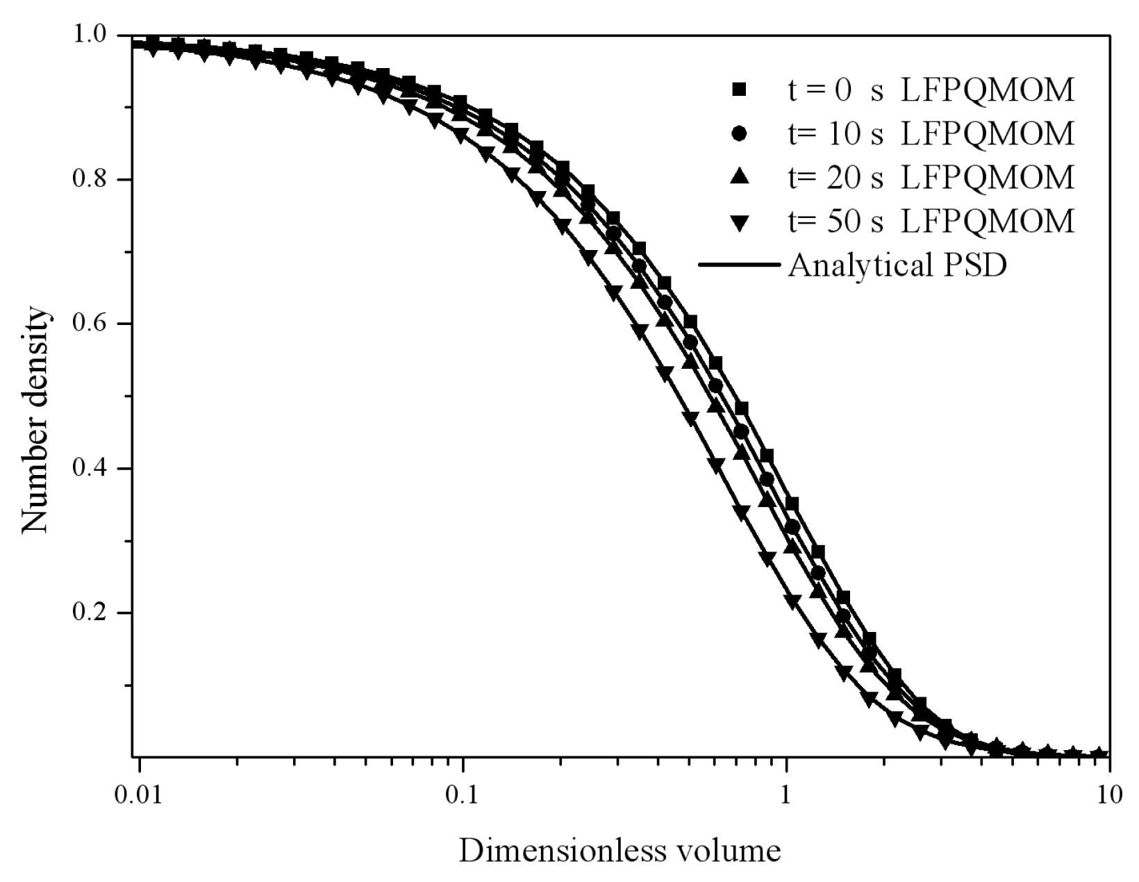
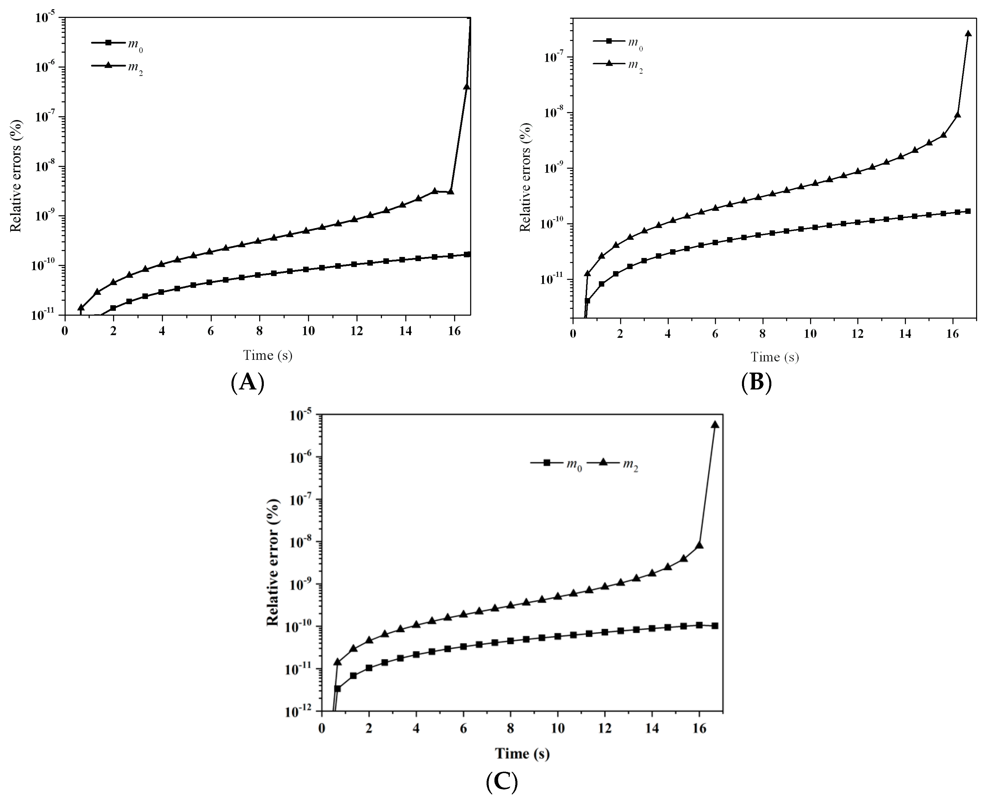
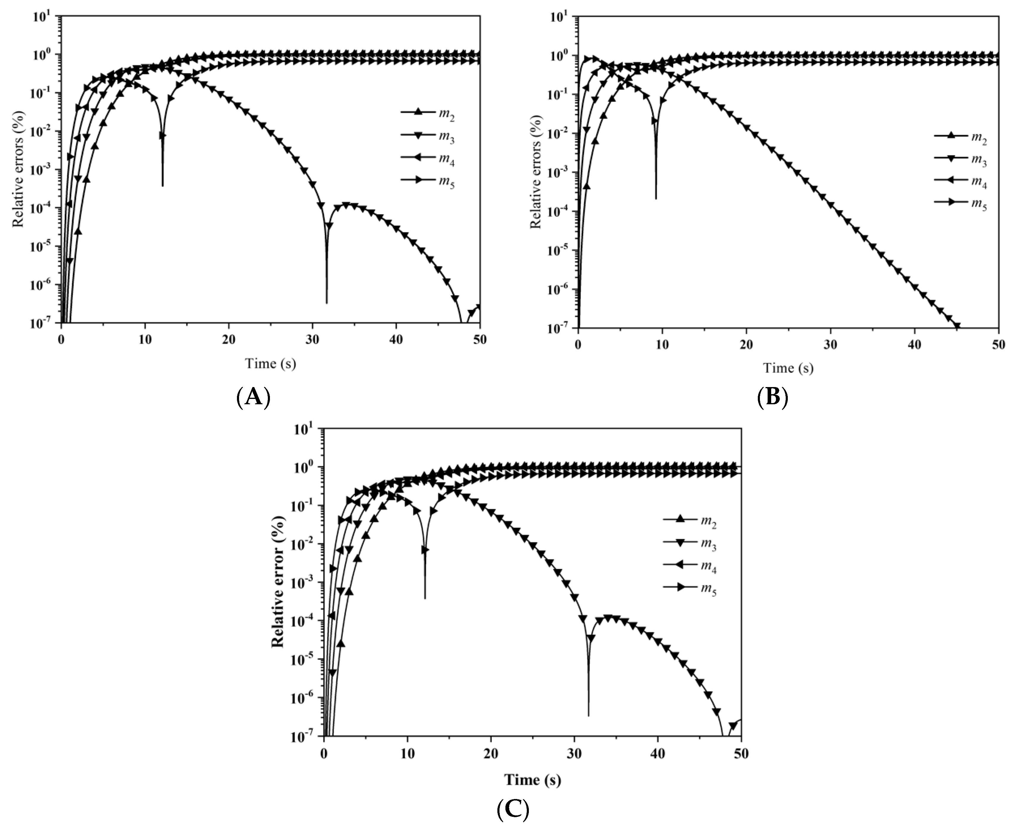
where , x = V/V0 and Γ (x) is the gamma function. The analytical moments are listed in Table 1. The gelling time tgel was 16.67 s. Similar to the previous case, two nodes were adopted with QMOM and three pivots in each section with LFPQMOM to track the moments exactly. Figure 11 depicts the evolution of the relative errors for the first six moments predicted by: (A) LFPQMOM; (B) QMOM; and (C) FPQMOM. The gelling time was 16.67 and a simulation time of 16.67 − Δt (=16.66) could be carried out with the new method, when m3 diverged. A maximum simulation time of 16.65 s could only be adopted with QMOM. Within a simulation of 16.65 s, the percentage errors with both methods were comparable, which were lower than 10−6%, but, after that time, QMOM was not appropriate for this test case. Similar to the previous case, the relative errors for m2 near the gelling point rose sharply. The relative errors for m1 were not included in the figure for their low values. Again, numerical errors with FPQMOM were similar to LFPQMOM. Figure 12 gives the particle size distributions at 0, 2, 10, and 16.66 s predicted by LFPQMOM along with their analytical counterparts for comparison. The numerical PSDs were in excellent agreement with the analytical PSDs on all the time points sampled. The computational time was about 46,042, 2818, and 996 ms for LFPQMOM, QMOM, and FPQMOM, respectively, in this test.
4.2. Pure Breakage
Three test cases were conducted for the pure breakage process. In the first test case, constant breakage kernel was adopted, i.e.,
with C0 = 0.1. Uniform distribution was used as the daughter distribution
Using Equation (36) with N0 = 1 and V0 = 1 as the initial distribution, the analytical solution for the moments was given by [22]
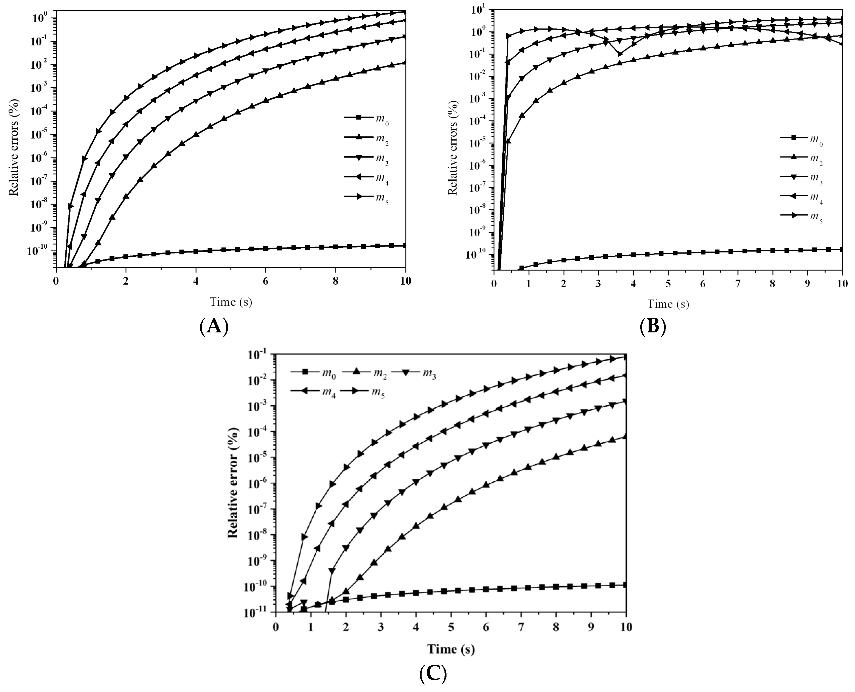
Unfortunately, analytical PSD was not available in this test case. Figure 13 shows the evolution of the relative errors for the first six moments predicted by: (A) LFPQMOM; (B) QMOM; and (C) FPQMOM. It was observed that the evolutions of the percentage errors of LFPQMOM and QMOM were very similar. The relative errors rose sharply initially and leveled off after 15 s. Lower rank moments had bigger numerical errors and within the simulation time, the relative errors for all the moments were lower than 2 × 10⁻⁹%. The percentage errors for m3 were not included in the figure due to their low values. Similar to the previous cases, m3 could be predicted without any error with the new method. Numerical predictions with FPQMOM were the best in this test. Figure 14 depicts the particle size distribution at 0, 2, 10, and 50 s. Due to lack of analytical PSD, a comparison of the numerical PSDs with their analytical counterparts was impossible, and thus, in this test case, only numerical PSDs are given at 2, 10, and 50 s. The computational time was about 14,850, 1037, and 345 ms for LFPQMOM, QMOM, and FPQMOM, respectively, in this test.
In the second test case for breakage process, linear breakage kernel was used, i.e.,
with a0 = 0.1, together with a uniform daughter distribution, i.e., Equation (47), exponential initial distribution, i.e., Equation (36) with N0 = 1 and V0 = 1. Analytical solution was given by [22]
Moments can be evaluated by numerical integration or direct integration analytically. Percentage errors for the first six moments—predicted by: (A) LFPQMOM; (B) QMOM; and (C) FPQMOM—are shown in Figure 15. In Figure 15B, the relative errors for the moments predicted by QMOM rose sharply at incipient time, especially for larger rank moments, m4 and m5 for instance. However, with the new method, the relative errors rose relatively slowly at incipient time, as can be seen in Figure 15A. With the simulation time, the maximum error for all the moments with FPQMOM was 1.88% whereas with QMOM, the maximum was 3.66%. With the new method, the numerical accuracy was improved relative to QMOM in this test case. The relative errors for m0 were comparable. Again, with the new method, m1 was predicted without any error, but not with QMOM. Relative errors for m1 were not included in the figure. FPQMOM was again the best in numerical prediction, and the relative errors for all the moments were less than 0.1% within the simulation time. Figure 16 gives the particle size distribution at 0, 2, 5, and 10 s, from which we observed that the numerical predictions with the new method agreed very well with the analytical PSDs at the time sampled. The computational time was about 3020, 190, and 66 ms for LFPQMOM, QMOM, and FPQMOM, respectively, in this test.
In the third test case for pure breakage, the power kernel was used as the breakage kernel having the form
with C0 = 0.01. Uniform distribution was used for the daughter distribution, i.e., Equation (47), together with the exponential initial distribution, i.e., Equation (36) with N0 = 1 and V0 = 1. Analytical solution was given by [22]
The numerical method was used to evaluate the moments. Evolutions of the relative errors for the first six moments are shown in Figure 17A,B for LFPQMOM and QMOM, respectively. In the figure, it was observed that, with the new method, all the relative errors were lower than 0.3% before the time of 20 s, and then fluctuated for m4 and m5, and rose for m0–m3. Within the simulation time, all the relative errors were lower than 2%. However, with QMOM, all the relative errors for the moments except m0 and m1 rose up to 0.1 within 5 s initially. Within the simulation time, the maximum percentage error for all the moments was 13.8%. With the new method, the numerical accuracy was improved in this test case. Again, LFPQMOM made an exact prediction for m1, similar to the previous cases. The relative errors for m1 were not included in the figure. Again, LFPQMOM had the smallest errors. Similar to the third case for the aggregation process, the sharp drops in the relative errors were related to the numerical evaluation of the moments. Figure 18 depicts the particle size distribution predicted by LFPQMOM at 0, 10, 20, and 50 s along with analytical counterparts for comparison. The numerical predictions exactly agreed with the analytical PSDs at different time points. The computational time was about 15,050, 876, and 338 ms for LFPQMOM, QMOM, and FPQMOM, respectively, in this test.
4.3. Aggregation and Breakage
Two test cases were conducted to validate the new method for the aggregation and breakage combined processes. The resulting source for Equation (6) is the summation of Equations (28) and (31). In the first test case, a constant kernel for aggregation, i.e., Equation (35) with C0 = 1, a linear kernel for breakage, i.e., Equation (49) with a0 = 0.1, and uniform daughter distribution, i.e., Equation (47), along with the following initial particle size distribution were adopted
with N0 = 1, V0 = 1. In this test case, analytical PSD was available [23]
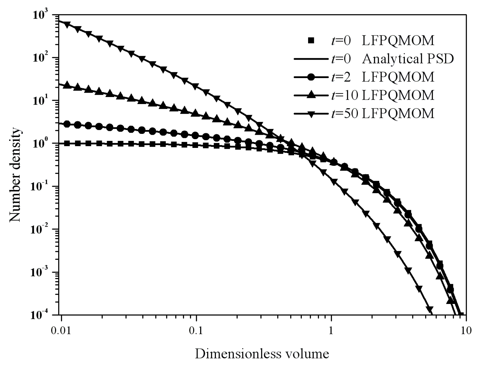
with Φ(τ) = Φ(∞)[1 + Φ(∞)tanh(Φ(∞)τ/2)]/[Φ(∞) + tanh(Φ(∞)τ/2)], Φ(∞) = (2a0V0/C0)1/2/N0, and τ = C0N0t. Moments could be evaluated analytically. Evolutions of percentage errors for the moments are shown in Figure 19 with: (A) LFPQMOM; (B) QMOM; and (C) FPQMOM. In the figure, the evolutions for the relative errors were very similar with the three methods. Initially, all the relative errors rose sharply and leveled off after the time of 20 s, except the errors for m3, which had a continuous drop as the time advanced. With the new method and FPQMOM, there were two fluctuations in the drop of relative errors for m3, but not with QMOM. Within the simulation time, the maximum relative error with both methods were comparable. In the figure, the relative errors for m0 and m1 were not included due to their low values. Figure 20 gives the particle size distributions at 0, 2, 10, and 50 s. It was observed that the numerical PSDs agreed very well with the analytical PSDs. Note that the PSD at 10 s coincided with the PSD at 50 s, proving that a steady state had been reached by the time of 10 s. Note that, with different physical parameters, the steady state can be different. The computational time was about 497,950, 32,275, and 10,374 ms for LFPQMOM, QMOM, and FPQMOM, respectively, in this test.
In the second test case for the aggregation and breakage combined process, a constant aggregation kernel was used, i.e., Equation (35) with C0 = 1, a linear kernel for breakage, i.e., Equation (49) with a0 = 0.25, and uniform daughter distribution, i.e., Equation (47), along with the following initial particle size distribution were adopted
with N0 = 1 and V0 = 2. When the following relation was satisfied, the analytical solution was available [23]
The analytical solution for particle size distribution was given by [23]
with K1(τ) = 7 + τ + exp(−τ), K2(τ) = 2 − 2exp(−τ), L2(τ) = 9 + τ − exp(−τ), p1,2 = 0.25(e−t−τ − 9 ± (d(τ))0.5), d(τ) = τ2 + (10τ − 2τe−τ) + 25 − 26e−τ + e−2τ, τ = C0N0t. The moments can be evaluated analytically.
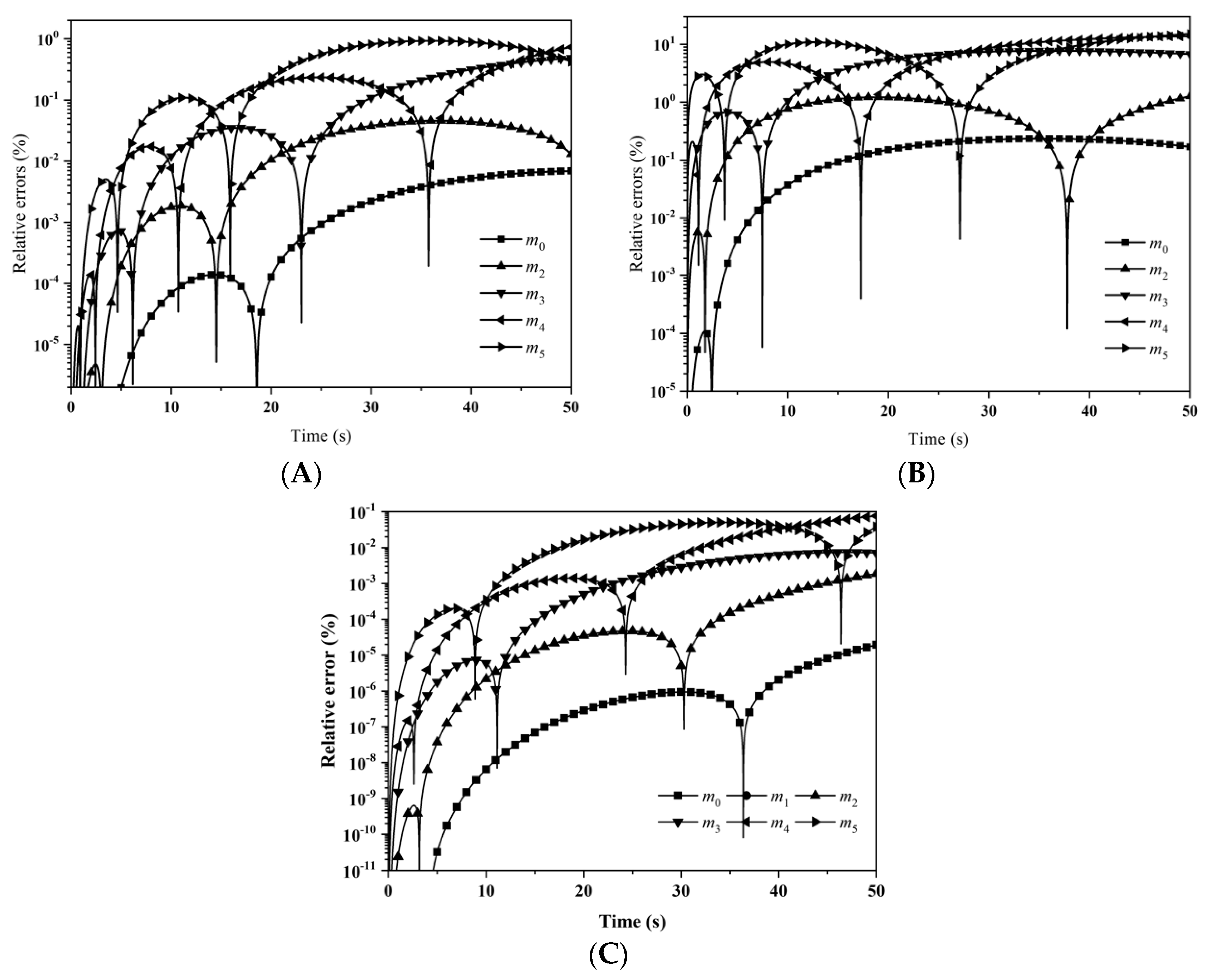
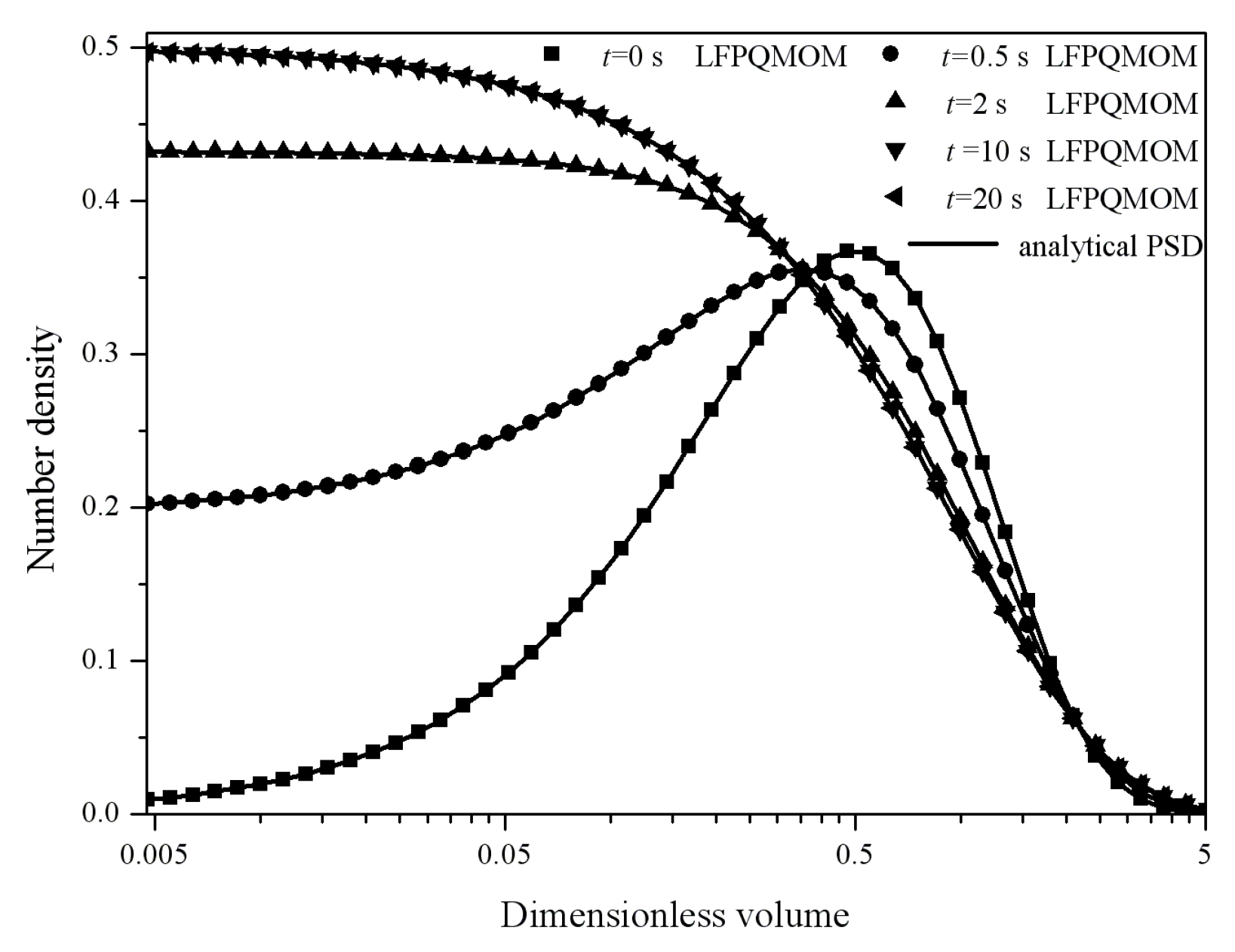
Figure 21 depicts the evolutions of percentage errors for m2–m5 with: (A) LFPQMOM; (B) QMOM; and (C) FPQMOM. The figure is very similar to the previous case. Initially, the errors rose sharply and leveled off for m2, m4, and m5, but decreased for m3 continuously. There was one difference from the previous case: the maximum percentage error was 0.42% with the new method, and 1.00% with QMOM. The numerical accuracy was improved with the new method relative to QMOM, which was similar to FPQMOM. Relative errors for m0 and m1 were not included in the figure given their low values. The numerical and the analytical particle size distributions at 0, 0.5, 2, 10, and 20 s are shown in Figure 22. The numerical PSDs agreed well with the analytical PSDs. The PSDs at 10 and 20 s coincided with each other, demonstrating that, by the time of 10 s, a steady state had been reached. Initially, the PSD was a Gaussian distribution, but, as the time advanced, the distributions became exponential, as can be seen in the figure. With the other parameters, the particle size distributions and the steady state could be different. The computational time was about 198,260, 12,048, and 4198 ms for LFPQMOM, QMOM, and FPQMOM, respectively, in this test.
5. Conclusions
In this work, a new numerical method, namely, the local fixed pivot quadrature method of moment (LFPQMOM) was proposed for the aggregation and breakage process. In the new method, particle size distribution in the local section was assumed to be a continuous summation of the Dirac Delta function with fixed pivots as performed in short time Fourier transformation (STFT). This assumption was applied to the sectional representation of aggregation or breakage, and the moments of the particle size distribution in the local domain were tracked successfully. The moments in the whole domain and the particle size distribution were constructed based on the moments in the local section without introducing further assumption.
Simulation of benchmark test cases including pure aggregation, pure breakage, and aggregation breakage combined process demonstrated that: (1) for the pure aggregation process, constant breakage process, and the aggregation and breakage combined process with exponential initial PSD, the accuracy of the prediction for the moments with the new method was comparable to quadrature method of moment (QMOM); (2) for the linear or square breakage process, and aggregation and breakage combined process with Gaussian initial PSD, the numerical accuracy for the moments was improved further; and (3) the new method could make good predictions for PSD in all of the test cases in this work.
A special algorithm was employed to solve the vandermode linear system, with which the coefficient matrix did not need to be constructed and, therefore, the influence of the ill-conditional feature of such a matrix on the numerical accuracy could be avoided. In theory, any number of moments can be tracked. Due to the large number of scalar equations included, the computational expense can be relatively large. Extension of the new algorithm to the solution of the multi-variable population balance equation will be investigated in depth in our future work.
Author Contributions
J.S., Z.G. and C.C. proposed the main framework of the paper. J.S. and W.L. mainly wrote the paper. C.C. proofread the paper.
Funding
This work was supported by the National Science and Technology Major Project of China (Grant No. 2016ZX05011001), the National Natural Science Foundation of China (Grant No. 41522504, 21306145), and the Key Laboratory of Ocean Energy Utilization and Energy Conservation of Ministry of Education (Grant No. LOEC-201803).
Conflicts of Interest
The authors declare no conflict of interest.
References
- Hounslow, M.J.; Ryall, R.L.; Marshall, V.R. A discretized population balance for nucleation, Growth, and Aggregation. AIChE J. 1988, 34, 1821–1832. [Google Scholar] [CrossRef]
- Kumar, S.; Ramkrishna, D. On the solution of population balance equations by discretization—I. A fixed pivot technique. Chem. Eng. Sci. 1996, 51, 1311–1332. [Google Scholar] [CrossRef]
- Kumar, S.; Ramkrishna, D. On the solution of population balance equations by discretization—II. A moving pivot technique. Chem. Eng. Sci. 1996, 51, 1333–1342. [Google Scholar] [CrossRef]
- Nicmanis, M.; Hounslow, M.J. Finite-element methods for steady-state population balance equations. AIChE J. 1998, 44, 2258–2272. [Google Scholar] [CrossRef]
- Rigopoulos, S.; Jones, A.G. Finite-element scheme for solution of dynamic population balance equation. AIChE J. 2003, 49, 1127–1139. [Google Scholar] [CrossRef]
- Qamar, S.; Warnecke, G. Solving population balance equations for two-component aggregation by a finite volume scheme. Chem. Eng. Sci. 2007, 62, 679–693. [Google Scholar] [CrossRef]
- McGraw, R. Description of aerosol dynamics by the quadrature method of moments. Aerosol Sci. Technol. 1997, 27, 255–265. [Google Scholar] [CrossRef]
- Rong, F.; Marchisio, D.; Fox, R.O. Application of the direct quadrature method of moments to polydisperse gas solid fluidized beds. Powder Technol. 2004, 139, 7–20. [Google Scholar]
- Su, J.W.; Gu, Z.L.; Li, Y.; Feng, S.Y.; Xu, X.Y. Solution of population balance equation using quadrature method of moments with an adjustable factor. Chem. Eng. Sci. 2007, 62, 5897–5911. [Google Scholar] [CrossRef]
- Su, J.W.; Gu, Z.L.; Li, Y.; Feng, S.Y.; Xu, X.Y. An adaptive direct quadrature metod of moment for Population Balance Equation. AIChE J. 2008, 54, 2872–2887. [Google Scholar] [CrossRef]
- Alopaeus, V.; Laakkone, N.M.; Aittamaa, J. Numerical solution of moment-transformed population balance equation with fixed quadrature points. Chem. Eng. Sci. 2006, 61, 4919–4929. [Google Scholar] [CrossRef]
- Gu, Z.L.; Su, J.W.; Jiao, J.Y.; Xu, X.Y. Simulation of Micro-behaviors Including Nucleation, Growth, Aggregation in Particle System. Sci. China Ser. B Chem. 2009, 52, 241–248. [Google Scholar] [CrossRef]
- Smith, M.; Matsoukas, T. Constant-number Monte Carlo simulation of population balances. Chem. Eng. Sci. 1998, 53, 1777–1786. [Google Scholar] [CrossRef]
- Tandon, P.; Rosner, D.E. Monte Carlo simulation of particle aggregation and simultaneous restructuring. J. Colloid Interface Sci. 1999, 213, 273–286. [Google Scholar] [CrossRef] [PubMed]
- Irizarry, R. Fast Monte Carlo methodology for multivariate particulate systems—I. Point ensemble Monte Carlo. Chem. Eng. Sci. 2008, 63, 95–110. [Google Scholar] [CrossRef]
- Attarakih, M.M.; Drumm, C.; Bart, H. Solution of the population balance equation using the sectional quadrature method of moments (SQMOM). Chem. Eng. Sci. 2009, 64, 742–752. [Google Scholar] [CrossRef]
- Gordon, R.G. Error bounds in equilibrium statistical mechanics. J. Math. Phys. 1968, 9, 655–663. [Google Scholar] [CrossRef]
- Golub, G.H.; Vanloan, C.F. Matrix Computations, 3rd ed.; Johns Hopkins University Press: Baltimore, MD, USA, 1996; pp. 183–188. [Google Scholar]
- Press, W.H.; Teukolsky, S.A.; Vetterling, W.T.; Flannery, B.P. Numerical Recipes in C++, 2nd ed.; Cambridge University Press: Cambridge, UK, 1992. [Google Scholar]
- Scott, W.T. Analytic studies of cloud droplet coalescence I. J. Atmos. Sci. 1968, 25, 54–65. [Google Scholar] [CrossRef]
- Smit, D.J.; Hounslow, M.J.; Paterson, W.R. Aggregation and gelation—I. Analytical solutions for CST and batch operation. Chem. Eng. Sci. 1994, 49, 1025–1035. [Google Scholar] [CrossRef]
- Ziff, R.M.; McGrady, E.D. The kinetics of cluster fragmentation and depolymerisation. J. Phys. A Math. Gen. 1985, 18, 3027–3037. [Google Scholar] [CrossRef]
- McCoy, B.J.; Madras, G. Analytical solution for a population balance equation with aggregation and fragmentation. Chem. Eng. Sci. 2003, 58, 3049–3051. [Google Scholar] [CrossRef]
Figure 1.
Contribution to the variation of m(t) in domain [a, b] due to aggregation.

Figure 2.
Contribution to the variation of m(t) in domain [a, b] due to aggregation.

Figure 3.
Evolution of the relative errors for the first six moments with: (A) LFPQMOM; (B) QMOM; and (C) FPQMOM (square: m0; up triangle: m2; down triangle: m3; left triangle: m4; right triangle: m5).
Figure 3.
Evolution of the relative errors for the first six moments with: (A) LFPQMOM; (B) QMOM; and (C) FPQMOM (square: m0; up triangle: m2; down triangle: m3; left triangle: m4; right triangle: m5).

Figure 4.
Particle size distribution predicted by LFPQMOM at 0, 2, 5, and 10 s (square: numerical PSD at 0 s; circle: numerical PSD at 2 s; up triangle: numerical PSD at 5 s; down triangle: numerical PSD at 10 s; line: analytical PSD).
Figure 4.
Particle size distribution predicted by LFPQMOM at 0, 2, 5, and 10 s (square: numerical PSD at 0 s; circle: numerical PSD at 2 s; up triangle: numerical PSD at 5 s; down triangle: numerical PSD at 10 s; line: analytical PSD).

Figure 5.
Evolution of relative errors for the first six moments with: (A) LFPQMOM; (B) QMOM; and (C) FPQMOM (square: m0; up triangle: m2; down triangle: m3; left triangle: m4; right triangle: m5).
Figure 5.
Evolution of relative errors for the first six moments with: (A) LFPQMOM; (B) QMOM; and (C) FPQMOM (square: m0; up triangle: m2; down triangle: m3; left triangle: m4; right triangle: m5).

Figure 6.
Particle size distributions at 0, 2, 5, and 10 s (square: numerical PSD at 0 s; circle: numerical PSD at 2 s; down triangle: numerical PSD at 5 s; up triangle: numerical PSD at 10 s; line: analytical PSD).
Figure 6.
Particle size distributions at 0, 2, 5, and 10 s (square: numerical PSD at 0 s; circle: numerical PSD at 2 s; down triangle: numerical PSD at 5 s; up triangle: numerical PSD at 10 s; line: analytical PSD).

Figure 7.
Evolution of the percentage errors for the first six moments with: (A) LFPQMOM; (B) QMOM; and (C) FPQMOM for the pure aggregation with sum kernel and exponential initial PSD (square: m0; circle: m1; up triangle: m2; down triangle: m3; left triangle: m4; right triangle: m5).
Figure 7.
Evolution of the percentage errors for the first six moments with: (A) LFPQMOM; (B) QMOM; and (C) FPQMOM for the pure aggregation with sum kernel and exponential initial PSD (square: m0; circle: m1; up triangle: m2; down triangle: m3; left triangle: m4; right triangle: m5).

Figure 8.
Particle size distribution at 0, 2, 10, and 30 s for the pure aggregation with sum kernel and exponential initial PSD (square: numerical PSD at 0 s; circle: numerical PSD at 2 s; up triangle: numerical PSD at 10 s; down triangle: numerical PSD at 30 s; line: analytical PSD).
Figure 8.
Particle size distribution at 0, 2, 10, and 30 s for the pure aggregation with sum kernel and exponential initial PSD (square: numerical PSD at 0 s; circle: numerical PSD at 2 s; up triangle: numerical PSD at 10 s; down triangle: numerical PSD at 30 s; line: analytical PSD).

Figure 9.
Evolution of percentage errors of m0 and m2 for the pure aggregation process with product kernel and exponential initial PSD: (A) LFPQMOM; (B) QMOM; and (C) FPQMOM (square: m0; up triangle: m2).
Figure 9.
Evolution of percentage errors of m0 and m2 for the pure aggregation process with product kernel and exponential initial PSD: (A) LFPQMOM; (B) QMOM; and (C) FPQMOM (square: m0; up triangle: m2).

Figure 10.
Particle size distribution at 0, 10, 20, and 50 s for the pure aggregation process with product kernel and exponential initial PSD (Square: numerical PSD at 0 s; circle: numerical PSD at 10 s; up triangle: numerical PSD at 20 s; down triangle: numerical PSD at 50 s; line: analytical PSD).

Figure 11.
Relative errors for m0 and m2 for the pure aggregation process with product kernel and Gaussian initial PSD with: (A) LFPQMOM; (B) QMOM; and (C) FPQMOM (square: m0; up triangle: m2).
Figure 11.
Relative errors for m0 and m2 for the pure aggregation process with product kernel and Gaussian initial PSD with: (A) LFPQMOM; (B) QMOM; and (C) FPQMOM (square: m0; up triangle: m2).

Figure 12.
Particle size distributions at 0, 2, 10, and 16.66 s for the pure aggregation process with product kernel and Gaussian initial PSD (square: numerical PSD at 0 s; circle: numerical PSD at 2 s; up triangle: numerical PSD at 10 s; down triangle: numerical PSD at 16.66 s; line: analytical PSD).

Figure 13.
Evolution of relative errors for the pure breakage process with constant kernel, exponential initial PSD, and uniform daughter distribution with: (A) LFPQMOM; (B) QMOM; and (C) FPQMOM (square: m0; up triangle: m2; down triangle: m3; left triangle: m4; right triangle: m5).
Figure 13.
Evolution of relative errors for the pure breakage process with constant kernel, exponential initial PSD, and uniform daughter distribution with: (A) LFPQMOM; (B) QMOM; and (C) FPQMOM (square: m0; up triangle: m2; down triangle: m3; left triangle: m4; right triangle: m5).

Figure 14.
Particle size distributions at 0, 2, 10, and 50 s for the pure breakage process with constant kernel, exponential initial PSD, and uniform daughter distribution (square: numerical PSD at 0 s; line: analytical PSD at 0 s; circle line: numerical PSD at 2 s; up triangle line: numerical PSD at 10 s; down triangle line: numerical PSD at 50 s).

Figure 15.
Evolution of the first six moments for the pure breakage process with linear kernel, exponential initial PSD, and uniform daughter distribution: (A) LFPQMOM; (B) QMOM; and (C) FPQMOM (square: m0; up triangle: m2; down triangle: m3; left triangle: m4 right triangle: m5).
Figure 15.
Evolution of the first six moments for the pure breakage process with linear kernel, exponential initial PSD, and uniform daughter distribution: (A) LFPQMOM; (B) QMOM; and (C) FPQMOM (square: m0; up triangle: m2; down triangle: m3; left triangle: m4 right triangle: m5).

Figure 16.
Particle size distribution at 0, 2, 5, and 10 s for the pure breakage process with linear kernel, exponential initial PSD, and uniform daughter distribution (square: numerical PSD at 0 s; circle: numerical PSD at 2 s; up triangle: numerical PSD at 5 s; down triangle: numerical PSD at 10 s; line: analytical PSD).

Figure 17.
Evolution of the relative errors for the first six moments for the pure breakage process with square kernel, exponential initial PSD, and uniform daughter distribution: (A) LFPQMOM; (B) QMOM; and (C) FPQMOM (square: m0; up triangle: m2; down triangle: m3; left triangle: m4; right triangle: m5).

Figure 18.
Particle size distribution at 0, 2, 5, and 10 s for the pure breakage process with square kernel, exponential initial PSD, and uniform daughter distribution (square: numerical PSD at 0 s; circle: numerical PSD at 10 s; up triangle: numerical PSD at 20 s; down triangle: numerical PSD at 50 s; line: analytical PSD).

Figure 19.
Relative errors for m2–m5 for the aggregation and breakage combined process with constant aggregation kernel, linear breakage kernel, uniform daughter distribution, and exponential initial PSD with: (A) LFPQMOM; (B) QMOM; and (C) FPQMOM (up triangle: m2; down triangle: m3; left triangle: m4; right triangle: m5).

Figure 20.
Particle size distributions at 0, 2, 10, and 50 s for the aggregation and breakage combined process with constant aggregation kernel, linear breakage kernel, uniform daughter distribution, and exponential initial PSD (square: numerical PSD at 0 s, Circle: numerical PSD at 2 s; up triangle: numerical PSD at 10 s; down triangle: numerical PSD at 50 s; line: analytical PSD).

Figure 21.
Evolutions for the relative errors of m2−m5 for the aggregation and breakage combined process with constant aggregation kernel, linear breakage kernel, uniform daughter distribution, and Gaussian initial particle size distribution: (A) LFPQMOM; (B) QMOM; and (C) FPQMOM (up triangle: m2; down triangle: m3; left triangle: m4; right triangle: m5).

Figure 22.
Particle size distributions at 0, 0.5, 2, 10, and 20 s for the aggregation and breakage combined process with constant aggregation kernel, linear breakage kernel, uniform daughter distribution, and Gaussian initial particle size distribution (square: numerical PSD at 0 s; circle: numerical PSD at 0.5 s; up triangle: numerical PSD at 2 s; down triangle: numerical PSD at 10 s; left triangle: numerical PSD at 20 s; line: analytical PSDs).


Table 1.
Analytical solution for the first three moments for the aggregation process with product kernel.
Table 1.
Analytical solution for the first three moments for the aggregation process with product kernel.
| Moments | Analytical Solution |
|---|---|
| m0(t) | |
| m1(t) | |
| m2(t) |
© 2018 by the authors. Licensee MDPI, Basel, Switzerland. This article is an open access article distributed under the terms and conditions of the Creative Commons Attribution (CC BY) license (http://creativecommons.org/licenses/by/4.0/).
Share and Cite
MDPI and ACS Style
Su, J.; Le, W.; Gu, Z.; Chen, C. Local Fixed Pivot Quadrature Method of Moments for Solution of Population Balance Equation. Processes 2018, 6, 209. https://doi.org/10.3390/pr6110209
AMA Style
Su J, Le W, Gu Z, Chen C. Local Fixed Pivot Quadrature Method of Moments for Solution of Population Balance Equation. Processes. 2018; 6(11):209. https://doi.org/10.3390/pr6110209
Chicago/Turabian StyleSu, Junwei, Wang Le, Zhaolin Gu, and Chungang Chen. 2018. "Local Fixed Pivot Quadrature Method of Moments for Solution of Population Balance Equation" Processes 6, no. 11: 209. https://doi.org/10.3390/pr6110209
Note that from the first issue of 2016, this journal uses article numbers instead of page numbers. See further details here.