High Mixing Efficiency by Modulating Inlet Frequency of Viscoelastic Fluid in Simplified Pore Structure
by
Meng Zhang
1,†, 
Yunfeng Cui
2,†,
Weihua Cai
1,*,
Zhengwei Wu
3,
Yongyao Li
1,
Fengchen Li
1,4 and
Wu Zhang
5,* 1
School of Energy Science and Engineering, Harbin Institute of Technology, Harbin 150001, China
2
School of Mechanical Engineering, Shanghai Jiao Tong University, Shanghai 200000, China
3
Department of Biomedical Engineering and Biotechnology, University of Massachusetts Lowell, Lowell, MA 01854, USA
4
Sino-French Institute of Nuclear Engineering and Technology, Sun Yat-Sen University, Zhuhai 519082, China
5
School of Electrical and Electronic Engineering, Nanyang Technological University, Singapore 639798, Singapore
*
Authors to whom correspondence should be addressed.
†
These authors contributed equally to this work.
Processes 2018, 6(11), 210; https://doi.org/10.3390/pr6110210
Submission received: 26 September 2018
/
Revised: 15 October 2018
/
Accepted: 16 October 2018
/
Published: 1 November 2018
(This article belongs to the Special Issue Fluid Flow in Fractured Porous Media)
Abstract
:Fluid mixing plays an essential role in microscale flow systems. Here, we propose an active mixing approach which enhances the mixing of viscoelastic fluid flow in a simplified pore T-junction structure. Mixing is actively controlled by modulating the driving pressure with a sinusoidal signal at the two inlets of the T-junction. The mixing effect is numerically investigated for both Newtonian and viscoelastic fluid flows under different pressure modulation conditions. The result shows that a degree of mixing as high as 0.9 is achieved in viscoelastic fluid flows through the T-junction mixer when the phase difference between the modulated pressures at the two inlets is 180°. This modulation method can also be used in other fluid mixing devices.
1. Introduction
Mixing processes aim to generate a homogenous solution of multiple components in natural and engineering flows [1,2]. Such processes have been widely applied in chemical analysis [3,4], biological analysis [5,6], heat and mass transfer for microfluidic devices [7,8], fluid dynamic analysis in a porous medium [9,10,11,12], and numerous relevant small-scale research areas [13,14,15]. Efficient mixing is often desired for complete interaction within multicomponent systems, microreaction platforms, and mixing and transfers of small volumes at pore-scales [16,17]. Mixing can be accomplished through chaotic flow or a turbulent flow [8,18,19]; however, due to the small-scales, such flows are difficult to achieve in microfluidic systems. The realization of turbulent flow in microchannels is much more complex and challenging than in larger tubes or in open space, where the flow rate is severely limited by the driving pressure. At low flow rates, where flows are often in the laminar, low Reynolds number regime, mixing must rely on molecular diffusion between the different fluid layers, the thicknesses of which are much larger than the characteristic diffusion length. Thus, instead of relying on inertial effects, other strategies to induce mixing, like introducing the elastic effect at microscale laminar flow, may enhance the mixing effect [20].
Many microfluidic designs use fluid mechanisms to overcome the absence of turbulence [8,18,21]. These mechanisms include splitting–recombining [22], twisting [23,24,25], transversal flows [9], vortices [26,27], and chaotic advection [1,28,29,30]. These strategies can be categorized into passive and active ways [2,31,32], which depend on the application of an external energy source. They operate by the same inherent principle to generate transversal components of velocity, causing the flow to become unstable, and the thickness of fluid layers to decrease.
Mixing is also a critical process in many subsurface engineering operations, such as oil recovery [29,33]. After a secondary recovery by water flooding of a subsurface hydrocarbon reservoir, the oil and aqueous phases coexist, and additional fluid may be injected to perform enhanced oil recovery (EOR). Fluids injected during EOR include surfactant solutions [34], polymer solutions [35], and aqueous nanoparticle suspensions [36,37], and the mixing of the new aqueous fluid with the previously-injected water is an important goal of the flooding operation. In particular, polymer solutions are always applied as the final chasing fluid following other EOR fluids [38] because the high viscosity of polymer solutions can effectively suppress viscous fingering and thereby stabilize the injection front [11,39,40]. Consequently, how the chasing polymer solution mixes with the preceding EOR fluids is important in determining the overall EOR efficiency. However, in addition to being highly viscous, polymer solutions can also be viscoelastic. Viscoelasticity has been shown to significantly affect flow in porous media [41,42,43,44] or even bring about local instabilities [41,45,46]. The instability of viscoelastic fluids in porous media has been widely observed, and presents a promising opportunity for enhanced mixing [47,48], but little is understood about how to actively control these instabilities to achieve this purpose.
In this paper, we modeled a T-junction chamber as a pore element to simulate the mixing effect of unstable viscoelastic fluid flows [49,50,51,52,53]. The instability of the viscoelastic fluid was induced by perturbing the flow through controlled driving pressures at the inlets. This mechanism can be considered an active method for the enhancement of mixing within a microfluidic channel when the flow state is laminar and uniaxial across the pore-like channel. The driving pressure at the two inlets of the mixer was modulated by time-dependent sinusoidal signals. The degree of mixing was compared under constant pressure as well as when the pressure was modulated in one or both inlets. The effects of amplitude, frequency, and phase difference of the driving pressures were compared for viscoelastic fluid flows and Newtonian fluid flows. Finally, the results were experimentally validated using a microfluidic device.
2. Numerical Schemes
2.1. Computational Model of T-Junction Micromixer
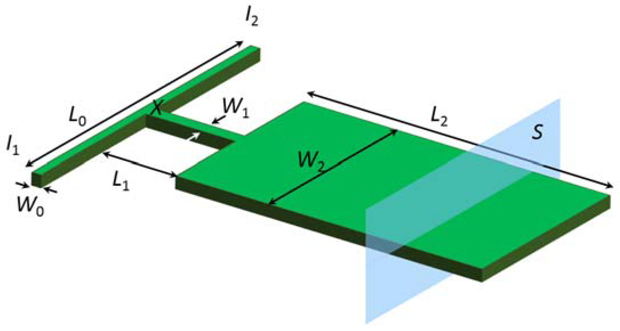
The computational model used in this study to simulate the T-junction micromixer is shown in Figure 1. Fluid components of different concentrations flow into two inlets I1 and I2 from both sides of the junction and convergence begins at the junction point X. Then, the mixing fluid flows through a narrow converging channel that feeds into an expanded mixing channel where the two fluids will mix with each other. The component concentration at a cross section S in the mixing channel is monitored to determine the mixing efficiency. The length and width of the inlet channels are L0 = 20 and W0 = 1, respectively, while the converging channel has dimensions of L1 = 6 and W1 = 0.5 and the mixing channel has L2 = 20 and W2 = 6. The micromixer structure has a depth of d = 1, and the outlet is set at the end of the mixing channel.
2.2. Governing Equations
Flows in the T-junction micromixer were investigated using a solver based on the open-source software OpenFoam. The velocity, pressure, and concentration fields were numerically simulated based on the fundamental governing equations. The continuous equation and Navier–Stokes (N–S) equation were applied to solve the incompressible Newtonian fluid flow:
where U represents the velocity vector of flow; p is the pressure; is the density; and is the dynamic viscosity of the fluid.
The convection–diffusion equation was applied to solve the component concentrations in the flow:
where C is the component concentration of the fluid and D is the diffusion coefficient of fluid.
For the incompressible viscoelastic fluid flow, the N–S equation is modified as:
where is the elastic stress, which can be derived from the constitutive equation of viscoelastic fluid. The constitutive equation describes the relation between molecule deformation and elastic stress in the fluid:
where kB is the Boltzmann constant; T is the absolute temperature of the fluid; is the Peterlin function; is the conformation tensor of polymer molecules; and is the Kronecker symbol for the unit tensor. The constitutive equation is further derived from Equation (5) as:
where is the solute viscosity and is the relaxation time of the solution. The transport equation of the conformation tensor is then expressed as:
where α is a parameter that relates to the anisotropy of drag encountered by flowing polymer segments [54]. Different and are selected in different constitutive models. Here, we assumed that the viscoelastic fluid is linearly extended during the flow, so that = 1 and = 0. This satisfies the flow situation of a Boger fluid in the Oldroyd-B constitutive model. Therefore, Equations (6) and (7) are simplified as:
Moreover, in order to gain more universal computational results, the dimensionless governing equations were used based on the following:
where H is the hydraulic diameter of the channel; Ui is the center velocity of the fluid at the inlet channel; ρ is the fluid density; and C is the component concentration in the fluid. We defined the dimensionless Reynolds number Re and Schmidt number Sc as:
where ν is the kinematic viscosity of the fluid. The dimensionless governing continuous equation and the N–S equation can then be expressed as:
and the convection–diffusion equation is expressed as:
Meanwhile, for a viscoelastic fluid, we defined the dimensionless parameter Weissenberg number Wi and the viscosity ratio β as:
where λ is the relaxation time of the viscoelastic fluid; ηp is the solute kinetic viscosity; ηs is the solvent kinetic viscosity. Thus, the dimensionless N–S equation for viscoelastic fluid flow and the conformation tensor transport equation are modified as:
For both Newtonian fluid and viscoelastic fluid cases, the dimensionless density, dimensionless viscosity, and Re were all set at 1.0, while Sc was set at 10−8. In addition, in the viscoelastic fluid case, the dimensionless relaxation time λ was set at 5.0, the dimensionless solution viscosity was set at 0.4, and dimensionless solvent viscosity was set at 0.6.
2.3. Numerical Methods
In this work, the fluid in the micromixer initially had a component concentration of 0. The dimensionless component concentration C1 was 0 for the fluid entering through inlet I1, while C2 = 1 for the fluid entering through inlet I2. The driving pressure is P1 at inlet I1 and P2 at inlet I2. The no-slip condition was imposed on all channel surfaces, and a fully developed flow condition was used at the mixer outlet.
The first-order Euler implicit scheme was used for time marching in the unsteady transport equations of Equations (14), (16), and (17), with a small dimensionless time step δt = 10−3. The convection terms in Equations (14) and (16) were discretized by the QUICK scheme, while the bounded MINMOD scheme was used to discretize the convection terms in Equation (17). Pressure–velocity coupling was handled by the PISO algorithm.
2.4. The Definition of Mixing Efficiency
Given component concentrations C1 = 0 and C2 = 1, a full mixing of the two fluids will result in a concentration of 0.5 when two averaged flow rates are the same. The degree of mixing is calculated by taking the standard deviation of concentration at all meshed points in cross-section S, defined as:
where N is the number of meshed points in the cross-section; is the concentration at point i; and E is the full mixing concentration, which is 0.5. Equation (18) is valid if the fluid density at each mesh point is the same. However, the flow rate is higher at the center of the channel and lower at the channel sides due to the no-slip boundary condition and fluid viscosity. Therefore, the deviation needs to be adjusted as:
where is the velocity at the mesh point i and is the average velocity in cross-section S. B ranges from 0 to 0.5, where B = 0 means full mixing while B = 0.5 indicates no mixing. We then define the degree of mixing as:
Therefore, M = 1 indicates full mixing, while M = 0 when no mixing occurs. We will use this index to present the mixing efficiency in the following sections.
3. Results and Discussion
3.1. Mixing in Condition of Constant Pressure
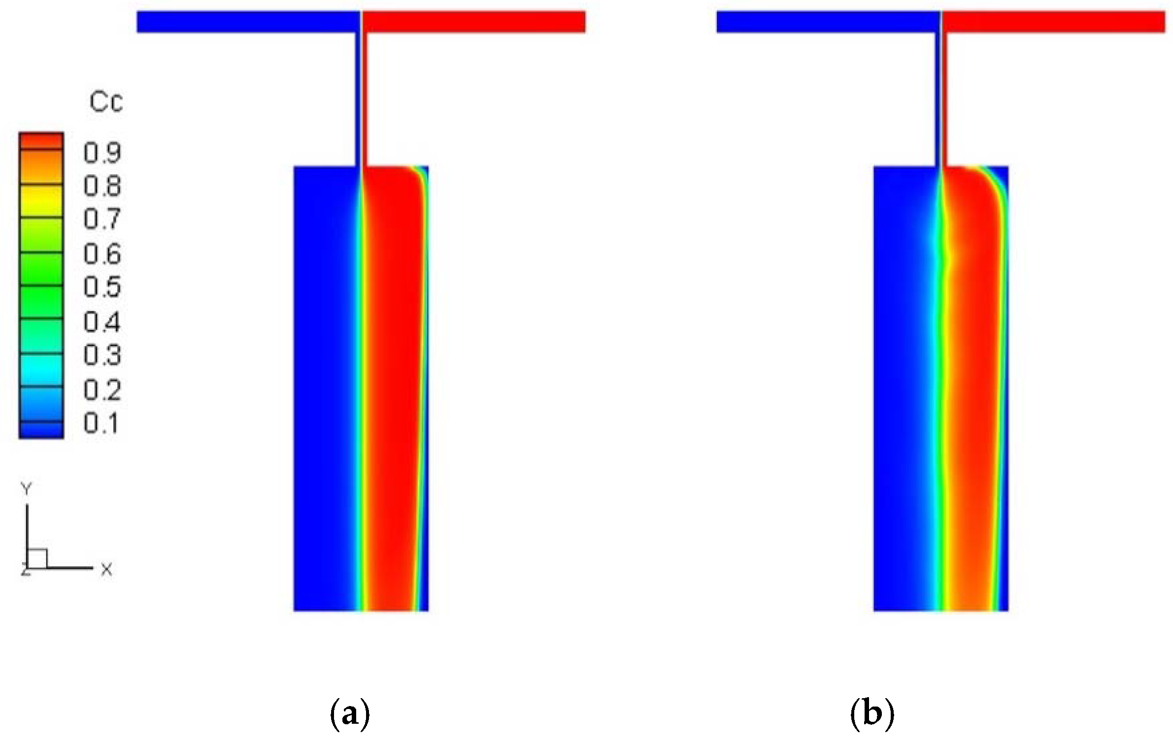
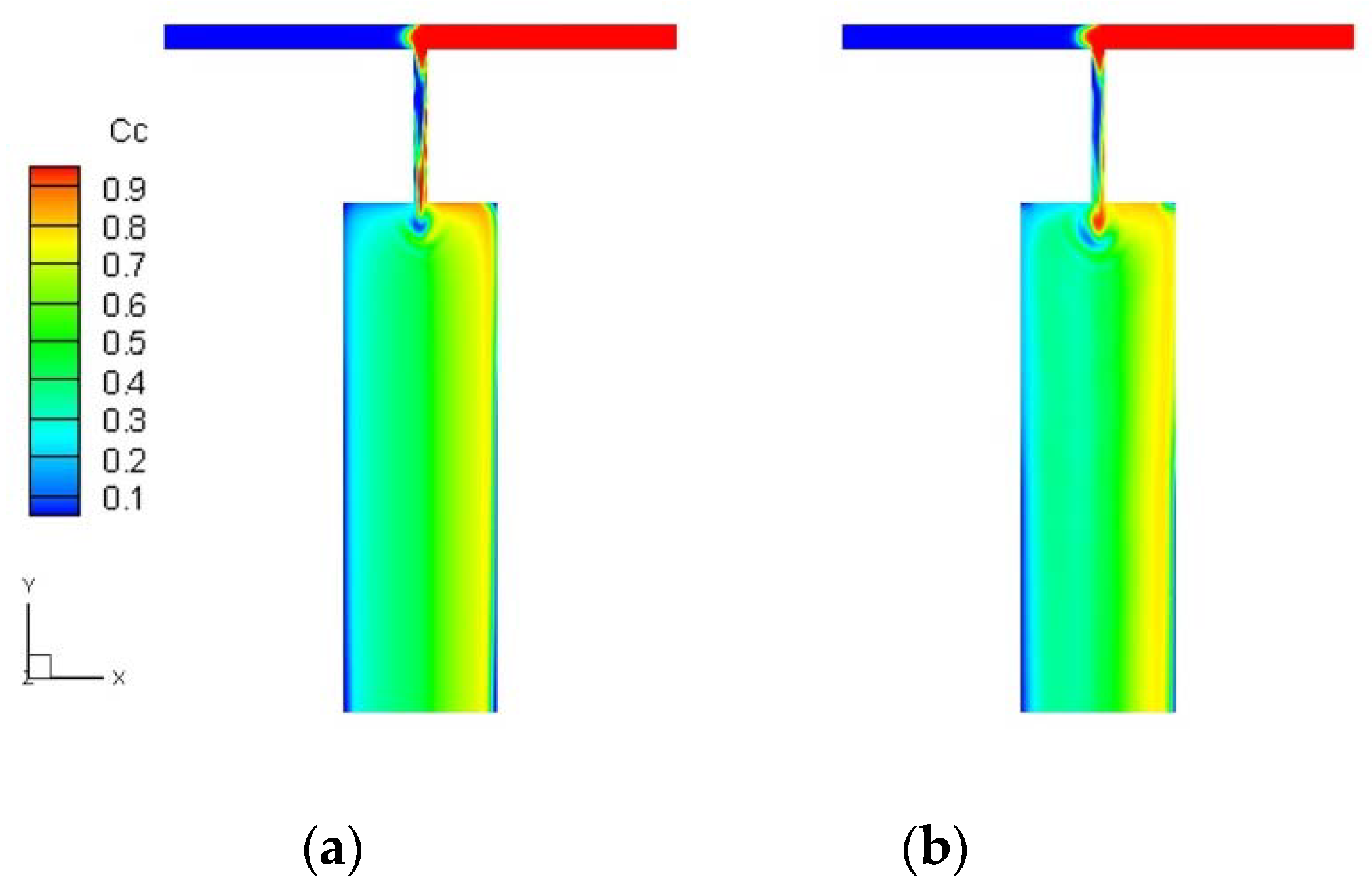
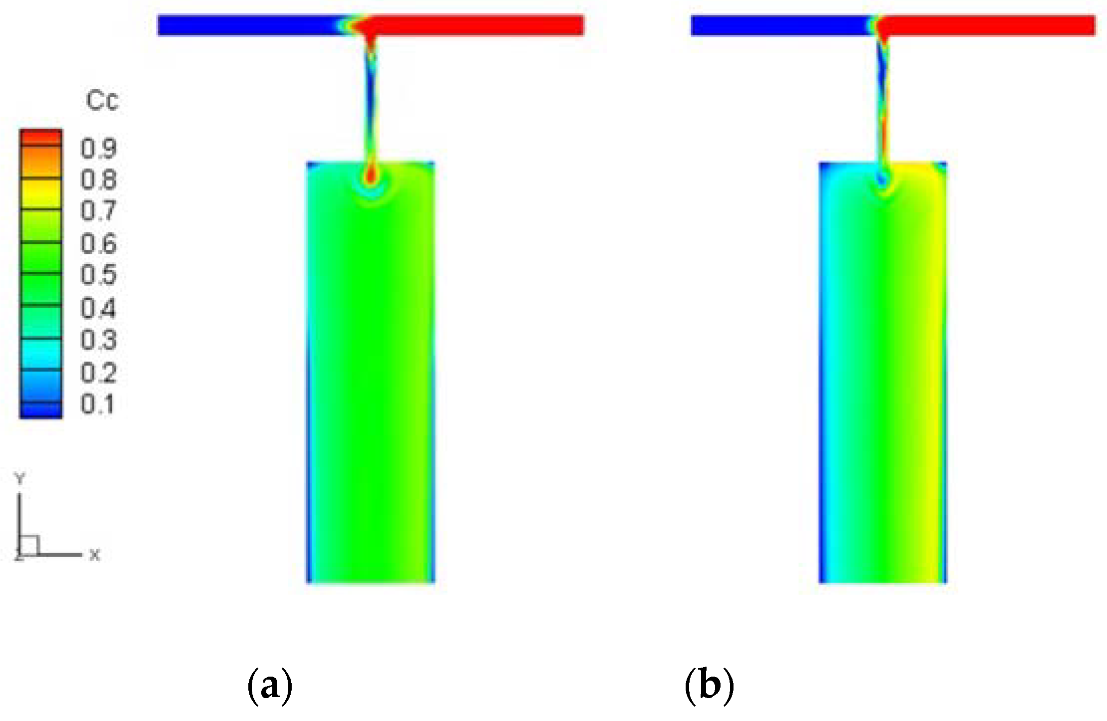
We first investigated fluid mixing in the T-junction micromixer when both inlets I1 and I2 are under the same constant pressure P0 = 3500. Figure 2a,b compare the component concentration distribution in the Newtonian fluid and viscoelastic fluid cases after the fluid has flowed in the micromixer for a long time (t = 120). The color map indicates the normalized component concentration (red represents C = 1 and blue represents C = 0). It can be seen that the two injected fluids are well separated in the converging channel. In the mixing channel, green appears at the center area along the flow direction. The concentration gradually changed between 0 and 1 and reached 0.5 in the center, indicating a high mixing here. Compared to the Newtonian fluid case, the mixing area is larger in the viscoelastic fluid. Since the simulation conditions for two fluids were identical except that the viscoelastic fluid had a nonzero elasticity, the improvement in mixing must originate from elastic stress in the viscoelastic fluid.
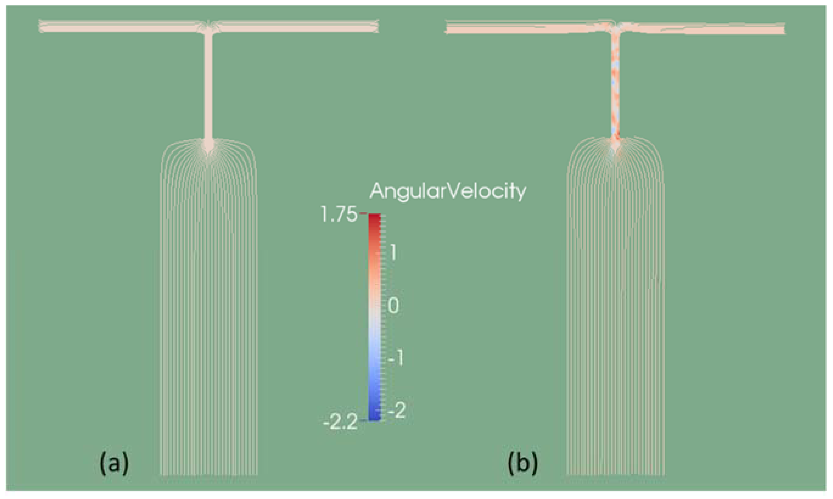
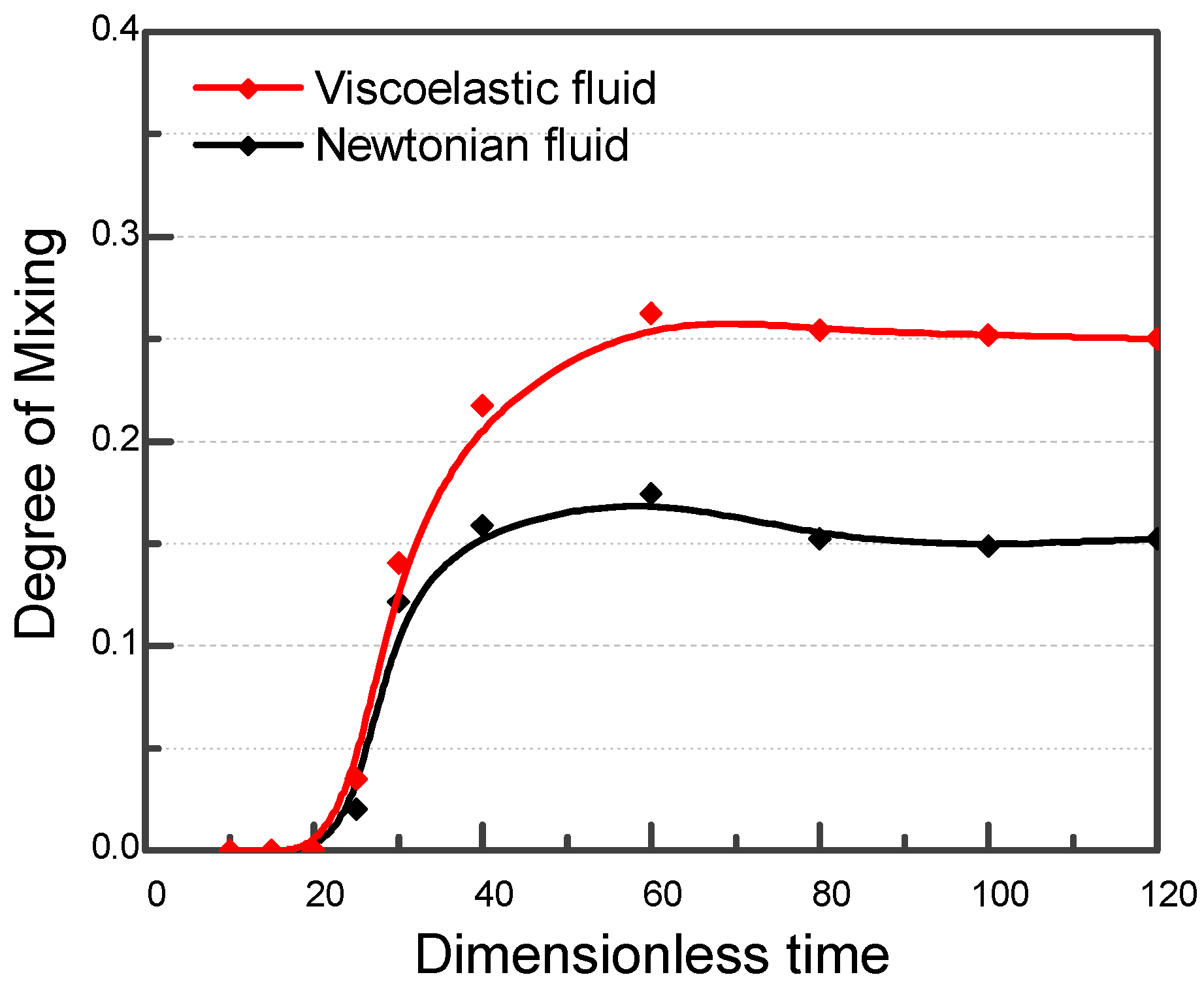
The elastic stress effect was further confirmed by investigating the flow streamlines and fluid angular velocity, as shown in Figure 3. In the Newtonian fluid case, the streamlines bend 90° downward at the convergence point and there is no angular velocity in the flow. By contrast, the streamlines in viscoelastic fluid in the same region first bend up slightly before bending down. A nonzero angular velocity is observed in the narrow channel, indicating convection of two viscoelastic fluids and more significant mixing. The degree of mixing M was analyzed at the cross-section S, which was set at a distance of Ls = 12 below the channel expansion point. For both cases, M increases until it becomes stable starting from t = 80, but their magnitudes differ: M plateaus at 0.15 for the Newtonian fluid case and 0.25 for the viscoelastic fluid case, as shown in Figure 4. This quantitatively shows that mixing was improved in viscoelastic fluid case.
3.2. Mixing in Single-Side Pressure Oscillation
We modulated the driving pressure P1 at inlet I1 with a sinusoidal factor while keeping the pressure P2 at inlet I2 constant:
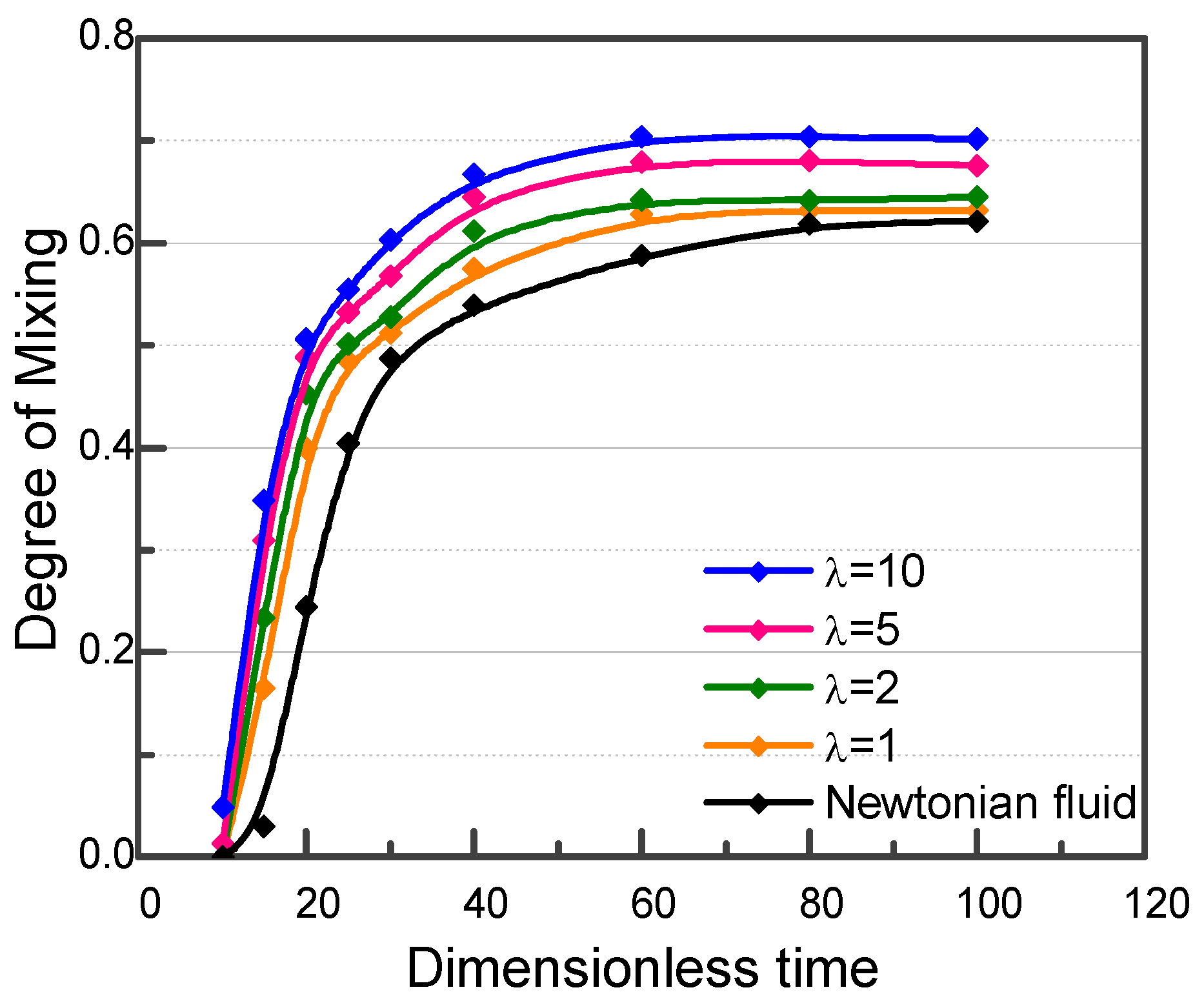
where A and f are the amplitude and frequency of the modulating signal, respectively. A, f, and P are all dimensionless. A was set at 0.8 to ensure a large pressure modulation while keeping the absolute pressure positive during the driving process. f was set at 1. P0 was the same as that in the constant pressure case, 3500. The change in the degree of mixing in cross-section S within one period was studied when pressures in Equation (21) were applied to the viscoelastic fluid case. Under the above driving pressure, the concentration distributions at t = 120 in the Newtonian fluid and viscoelastic fluid cases are shown in Figure 5, respectively. The transition region between the blue (low concentration) and red (high concentration) fluids expanded significantly when the pressure was modulated compared to when the pressure was constant, indicating that pressure modulation greatly improves mixing efficiency. Meanwhile, the concentrations in the converging channel were no longer uniformly distributed along the channel due to the pressure changes over time. At times P1 < P2, higher concentration fluid from inlet I2 will enter the converging channel. The converse happens when P1 > P2. In other words, the two fluids will alternatively enter the mixing channel in larger amounts. Due to the large width of the subsequent expanded channel, the small amounts of fluids introduced during one pressure cycle will start to expand and convect with each other. In this way, better mixing can be realized. In addition, we can also see that the larger discontinuous portion of fluid alternated more in the converging channel for the viscoelastic fluid case compared to the Newtonian fluid case, which indicates a higher mixing efficiency in the viscoelastic fluid. This was confirmed by investigating the degree of mixing at the cross-section S for both fluids. Figure 6 compares the mixing of a viscoelastic fluid with a different relaxation time and a Newtonian fluid. Mixing increased with the relaxation time and became stable at t = 80 for all fluids. The Newtonian fluid had the lowest degree of mixing of 0.62. Mixing gradually increased from 0.63 to 0.70 as the relaxation time λ increased from 1 to 10. This is because a higher relaxation time indicates a larger elastic stress, which leads to more convection in the fluid. Compared to the condition of constant pressure, the degree of mixing increased from 0.15 to 0.61 for the Newtonian fluid case under modulated pressure and from 0.25 to 0.68 for a viscoelastic fluid with λ of 5.
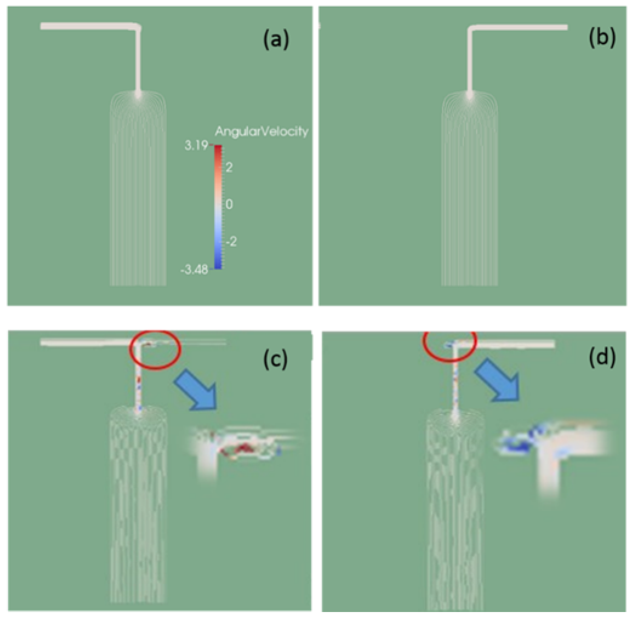
The flow streamlines and flow angular velocity were also investigated within one period, shown in Figure 7a,b for the Newtonian fluid case and Figure 7c,d for the viscoelastic fluid case. For both fluids, the stream flowed mainly from inlet I1 at t = 119.2 (Figure 7a,c) and mainly from inlet I2 at t = 119.7 (Figure 7b,d). The streamlines were smooth, and no angular velocity was observed in the Newtonian fluid case. However, the viscoelastic fluid formed flow vortexes alternating between the right and left sides of convergence points at times t = 119.2 and t = 119.7, respectively. The fluctuation in flow vortexes indicates enhanced convection between two fluids, which in turn leads to better mixing.
3.3. Mixing in Double-Sided Pressure Oscillation
Since a single inlet modulation improves mixing, we next investigated the effect of modulating the driving pressure at both inlets. Here, we modulated both driving pressures P1 and P2 with sinusoidal signals of the same amplitude A and frequency f, but with independent phase delays φ1 and φ2:
and we examined the dependence of mixing on A, f, and Δφ = φ1 − φ2, the phase difference between the two pressures.
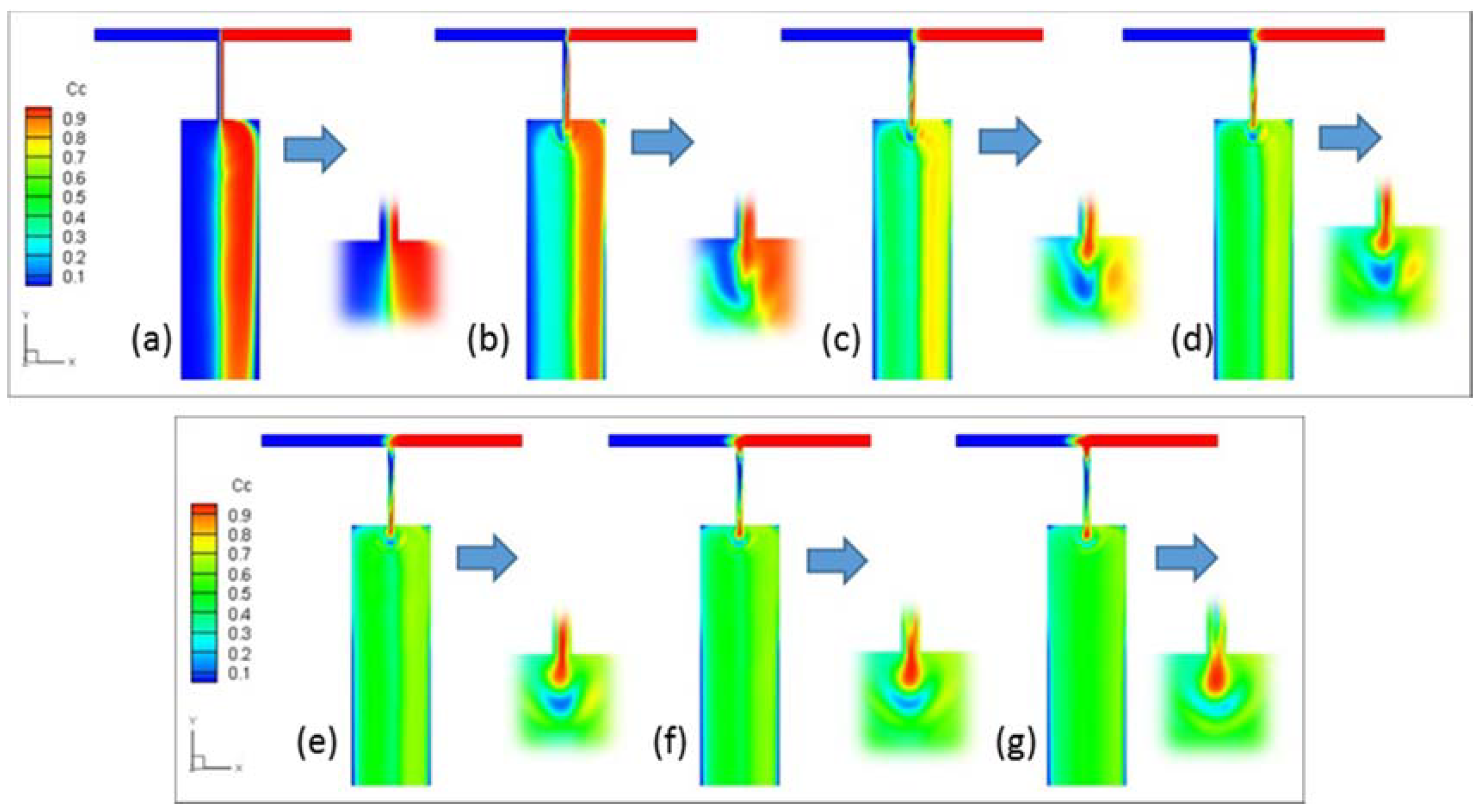
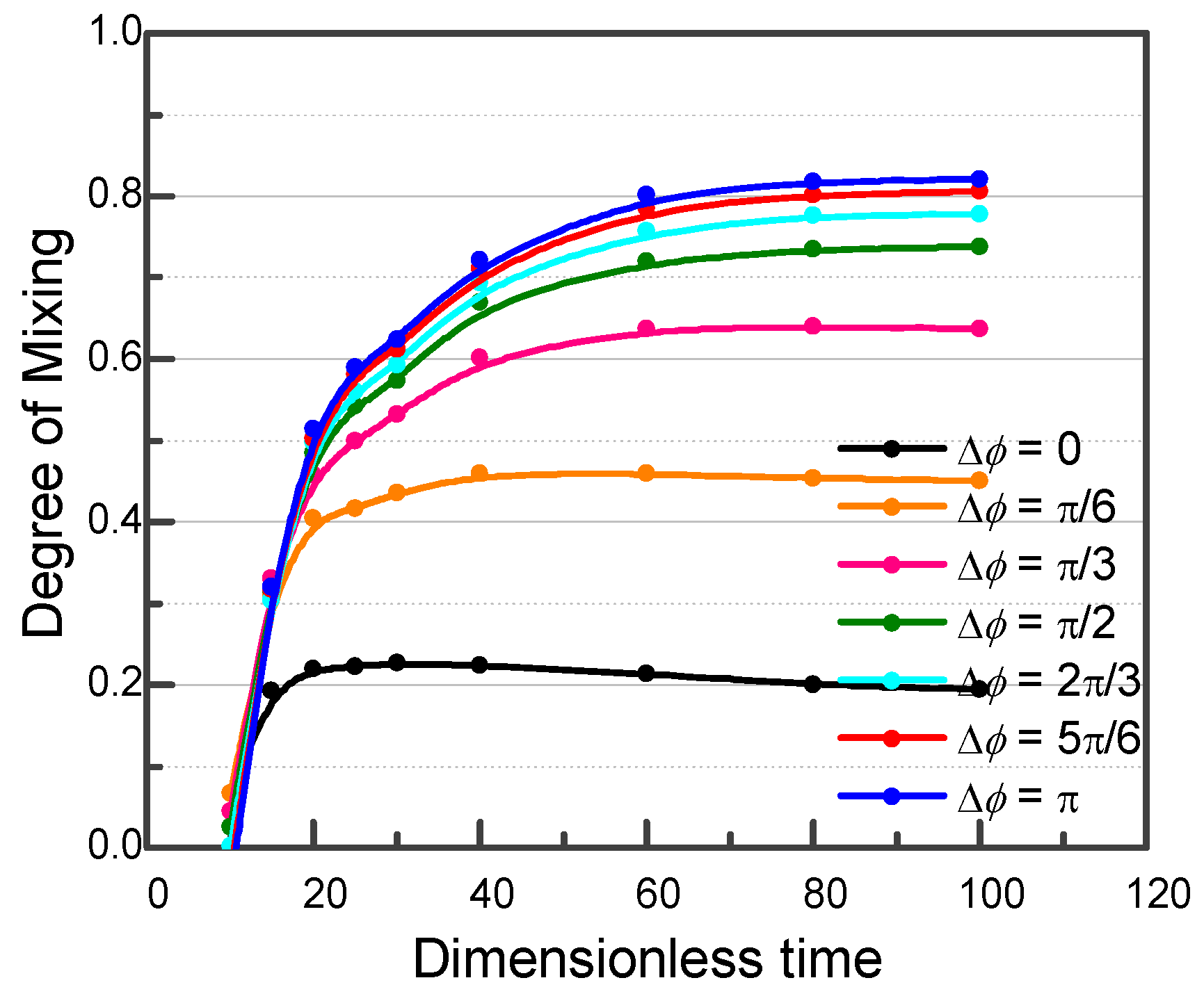
Setting A = 3500 and f = 1, the concentration distribution of viscoelastic fluid when Δφ varies from 0 to π was investigated at t = 120, shown in Figure 8. The high and low concentration fluids are symmetrically distributed on both sides of the T-junction when Δφ = 0 (Figure 8a) because the driving pressure at both inlets is always the same. Only very small amounts of the two fluids mix with each other along the center of the channel. However, the distribution symmetry is broken as Δφ starts to increase. A small fluctuation of the fluids in the converging channel was observed when Δφ = π/6, and it was magnified at the expansion point when the fluids entered the expanded channel, as shown in Figure 8b. As a consequence, the size of the mixing region starts to increase. As Δφ is increased to π/3, the two fluids start to alternate along the converged channel (Figure 8c) and the blue and red flows start to become discontinuous at the expansion point. Furthermore, the green region increases, while narrow streams of the low and high concentration fluids remain observable near the left and right sidewalls, respectively. As Δφ is further increased to π/2 (Figure 8d), the green region occupies most of the expansion channel, and isolated spots of unmixed fluid appear at the expansion point, as shown in the insert of Figure 8d. This means that the instantaneous pressure difference between the two inlets was large enough to allow the fluids to enter the converged channel separately. For Δφ between 2π/3 to π (Figure 8e–g), the green region occupies almost all of the expansion channel, indicating good mixing. The degree of mixing for different Δφ is plotted in Figure 9. When Δφ = 0, the mixing degree stabilizes at 0.2 after t = 20. The stabilization time t increases to 40, 60 and 80 for Δφ of π/6, π/3, and π/2, respectively, and the corresponding maximum degrees of mixing increase to 0.45, 0.63 and 0.73, respectively. The degree of mixing reaches a system-wide maximum value of 0.82 when Δφ = π. A phase difference of π maximizes the difference in the amount of fluid entering from each inlet at any instant in time. The fluid volumes alternate during each period, and this alternating fluid pattern expands in the wide mixing channel. As a result, the diffusion area is increased. By contrast, when Δφ = 0, the fluids from the inlets flow side by side along the channel direction and the diffusion area is only along the length of the center line.
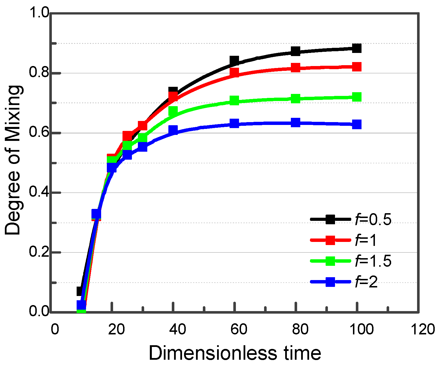
At a higher frequencies, less fluid will enter the converged channel during each period. As shown in Figure 10a,b, the component mixing maps are compared for the viscoelastic fluid case when f = 1 and f = 1.5, respectively, with fixed parameters A = 3500 and Δφ = π. The green region shrinks significantly when f increases from 1 to 1.5. In addition, larger regions of unmixed fluid occupy the left and right sides of the expanded channel. This indicates that a higher modulating frequency undermines the mixing effect. This can be better understood by looking at the concentration distributions in the inlets and in the converging channel. At time t = 120, the pressure at inlet I2 is higher than that at inlet I1, and more of the red fluid will be injected. At a lower modulating frequency, the difference in the amount of fluid flowing into the converging channel from each side is larger in each cycle; this can be observed in the converging channel and results in a higher mixing efficiency overall. The final degrees of mixing, which increase from 0.61 to 0.90 as the pressure oscillation frequency decreases from f = 2 to f = 0.5, are shown in Figure 11.
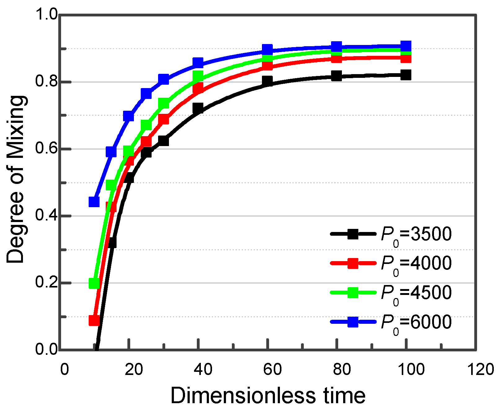
In addition, we can also increase the degree of mixing by increasing the alternating volume within one cycle using a higher pressure level at the inlets. To do this, P0 in Equation (22) is varied between 3500 to 6000 while setting f = 1 and Δφ = π. By increasing P0, the final degree of mixing in the viscoelastic fluid case also increases from 0.82 to 0.91, as shown in Figure 12.
4. Experimental Results
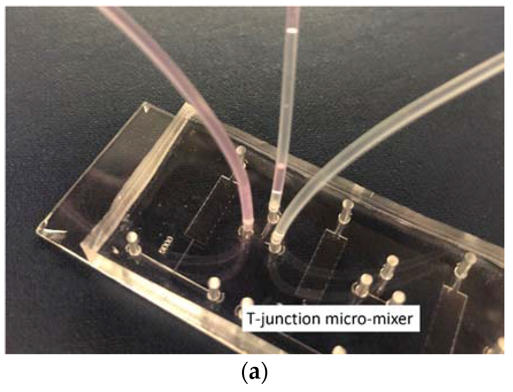
To validate the results of the simulations, the mixing efficiency was experimentally studied here in a PDMS-glass bonded microfluidic chip, as shown in Figure 13a. A mold for the PDMS structure was fabricated from SU8 photoresist on a silicon wafer using a standard photolithography process. The PDMS is a mixture of base and crosslinker with a ratio of 10:1. It was poured on the SU8 mold and cured at 65 °C for 4 h. To complete the chip, the cured PDMS was bonded to a glass slide after oxygen plasma treatment. The size of the microchannel was scaled to 100 µm based on the model in Figure 1. The length and width of the inlet channel were L0 = 2 mm and W0 = 100 µm, respectively. The converging channel was L1 = 600 µm in length and W1 = 50 µm in width. The mixing channel was L2 = 2 mm in length and W2 = 600 µm in width. The entire micromixer structure had a depth of d = 100 µm, and the outlet was directly at the end of the mixing channel.
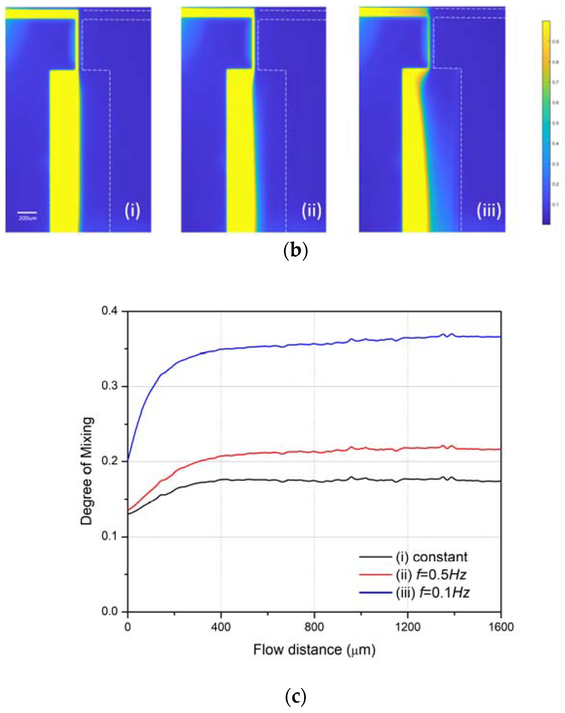
A Newtonian glycerol solution was injected into the two inlets of the T-junction mixer. The fluid at one inlet contained 10 µg/mL of Rhodamine B, while the other did not, so the mixing degree could be determined by quantifying the Rhodamine B concentration. With the limit of one programmable pump (PHD ULTRATM 4400), we fixed the flow rate at 500 µL/h on one inlet, and modulated the flow rate on the other side under three different conditions: (i) Constant flow rate of 500 µL/h; (ii) alternating flow rate between 0 and 1000 µL/h at a frequency f = 0.5 Hz and duty cycle of 50%; (iii) alternating flow rate between 0 and 1000 µL/h at a frequency f = 0.1 Hz and duty cycle of 50%. The recorded flow pattern is shown in Figure 13b. The color map represents the Rhodamine B concentration, which is normalized from 0 to 1: Yellow denotes a concentration of 1 and blue, a concentration of 0. For case (i), the flow rates at both inlets were the same constant value and the mixing region was narrow, indicating a small degree of mixing. For case (ii), the mixing region was increased when the flow rate on one side alternated at f = 0.5 Hz. The mixing region was further increased when the frequency decreased to 0.1 Hz in case (iii). According to the normalized concentrations of Rhodamine B, the degree of mixing at different flow distances along the channel is calculated using Equation (20) and plotted in Figure 13c. The origin indicates the point at which the fluid enters the mixing channel. The degree of mixing gradually increases with the flow distance, and stabilizes at 0.20 for case (i), 0.25 for case (ii), and 0.37 for case (iii). This experimentally demonstrates the enhancement in mixing when the flow is modulated on one side compared to having a constant driving flow at both sides, which agrees well with the simulation results. This also confirms that mixing is increased as the alternating frequency decreases.
5. Conclusions
In conclusion: A T-junction micromixer was modeled, and mixing efficiencies were numerically compared for both a Newtonian fluid and a viscoelastic fluid as a function of driving pressure amplitude and modulation frequency. The degree of mixing is higher in a viscoelastic fluid than in a Newtonian fluid due to elastic stress in the viscoelastic fluid. Different modulations of the driving pressures at each inlet of the micromixer were explored. Under constant driving pressures, the degree of mixing was relatively low, 0.15 for the Newtonian fluid case and 0.25 for the viscoelastic fluid case. When the driving pressures were modulated with a sinusoidal factor at one inlet while being held constant at the other, the degree of mixing increased to 0.62 and 0.67 for the Newtonian fluid and the viscoelastic fluid, respectively. When the driving pressures at both inlets of the micromixer were modulated with a sinusoidal factor, the mixing efficiency could be increased significantly by controlling the phase difference between the modulated pressures. The degree of mixing reached a maximum value of 0.82 using a viscoelastic fluid with a phase difference of π. Mixing enhancement arising from a low-frequency, single-inlet alternating modulation of the flow rate was experimentally demonstrated for a Newtonian glycerol solution. The method of modulating the driving pressure to enhance mixing may have potential applications in chemical engineering and in flow through porous media.
Author Contributions
M.Z. raised the original idea, wrote part of code for simulation software, analyzed the data, carried on the experiment, and wrote the paper. Y.C. simulated the data. W.C. revised the paper and coordinated this work. Z.W. did the experiment. Y.L. simulated the data. F.L. supervised on the simulation and the code for simulation software. W.Z. discussed the original idea, analyzed the simulation and experimental data, composed, and revised the paper.
Funding
This work is supported by this project is supported by the China Scholarship Council (No. 201606120130).
Conflicts of Interest
The authors declare no conflicts of interest.
References
- Stroock, A.D.; Dertinger, S.K.W.; Ajdari, A.; Mezić, I.; Stone, H.A.; Whitesides, G.M. Chaotic mixer for microchannels. Science 2002, 295, 647–651. [Google Scholar] [CrossRef] [PubMed]
- Lee, C.Y.; Fu, L.M. Recent advances and applications of micromixers. Sens. Actuators B Chem. 2018, 259, 677–702. [Google Scholar] [CrossRef]
- Roberge, D.M.; Ducry, L.; Bieler, N.; Cretton, P.; Zimmermann, B. Microreactor technology: A revolution for the fine chemical and pharmaceutical industries? Chem. Eng. Technol. 2005, 28, 318–323. [Google Scholar] [CrossRef]
- Ehrfeld, W.; Hessel, V.; Löwe, H. Microreactors—New Technology for Modern Chemistry; Wiley-VCH: Weinheim, Germany, 2000; p. 288. ISBN 3-527-29590-9. [Google Scholar]
- Kefala, I.N.; Papadopoulos, V.E.; Karpou, G.; Kokkoris, G.; Papadakis, G.; Tserepi, A. A labyrinth split and merge micromixer for bioanalytical applications. Microfluid. Nanofluid. 2015, 19, 1047–1059. [Google Scholar] [CrossRef]
- Lang, Q.; Ren, Y.; Hobson, D.; Tao, Y.; Hou, L.; Jia, Y.; Hu, Q.; Liu, J.; Zhao, X.; Jiang, H. In-plane microvortices micromixer-based AC electrothermal for testing drug induced death of tumor cells. Biomicrofluidics 2016, 10, 64102. [Google Scholar] [CrossRef] [PubMed] [Green Version]
- Hessel, V.; Löwe, H.; Schönfeld, F. Micromixers—A review on passive and active mixing principles. Chem. Eng. Sci. 2005, 60, 2479–2501. [Google Scholar] [CrossRef]
- Abed, W.M.; Whalley, R.D.; Dennis, D.J.C.; Poole, R.J. Experimental investigation of the impact of elastic turbulence on heat transfer in a serpentine channel. J. Non-Newtonian Fluid Mech. 2016, 231, 68–78. [Google Scholar] [CrossRef]
- Ye, Y.; Chiogna, G.; Cirpka, O.A.; Grathwohl, P.; Rolle, M. Experimental investigation of transverse mixing in porous media under helical flow conditions. Phys. Rev. E 2016, 94, 13113. [Google Scholar] [CrossRef] [PubMed]
- Ouyang, Y.; Xiang, Y.; Zou, H.; Chu, G.; Chen, J. Flow characteristics and micromixing modeling in a microporous tube-in-tube microchannel reactor by CFD. Chem. Eng. J. 2017, 321, 533–545. [Google Scholar] [CrossRef]
- Li, J.S.; Li, Q.; Cai, W.H.; Li, F.C.; Chen, C.Y. Mixing Efficiency via Alternating Injection in a Heterogeneous Porous Medium. J. Mech. 2018, 34, 167–176. [Google Scholar] [CrossRef]
- Cai, J.; Wei, W.; Hu, X.; Liu, R.; Wang, J. Fractal characterization of dynamic fracture network extension in porous media. Fractals 2017, 25. [Google Scholar] [CrossRef]
- Elvira, K.S.; Solvas, X.C.; Wootton, R.C.R.; Demello, A.J. The past, present and potential for microfluidic reactor technology in chemical synthesis. Nat. Chem. 2013, 5, 905–915. [Google Scholar] [CrossRef] [PubMed]
- Floquet, C.F.A.; Sieben, V.J.; MacKay, B.A.; Mostowfi, F. Determination of boron concentration in oilfield water with a microfluidic ion exchange resin instrument. Talanta 2016, 154, 304–311. [Google Scholar] [CrossRef] [PubMed]
- Liu, R.; Jiang, Y.; Li, B.; Wang, X. A fractal model for characterizing fluid flow in fractured rock masses based on randomly distributed rock fracture networks. Comput. Geotech. 2015, 65, 45–55. [Google Scholar] [CrossRef] [Green Version]
- Knight, J.B.; Vishwanath, A.; Brody, J.P.; Austin, R.H. Hydrodynamic focusing on a silicon chip: Mixing nanoliters in microseconds. Phys. Rev. Lett. 1998, 80, 3863–3866. [Google Scholar] [CrossRef]
- Squires, T.M.; Quake, S.R. Microfluidics: Fluid physics at the nanoliter scale. Rev. Mod. Phys. 2005, 77, 977–1026. [Google Scholar] [CrossRef] [Green Version]
- Xia, H.M.; Wang, Z.P.; Koh, Y.X.; May, K.T. A microfluidic mixer with self-excited ‘turbulent’ fluid motion for wide viscosity ratio applications. Lab Chip 2010, 10, 1712–1716. [Google Scholar] [CrossRef] [PubMed]
- Lemenand, T.; Della Valle, D.; Habchi, C.; Peerhossaini, H. Micro-mixing measurement by chemical probe in homogeneous and isotropic turbulence. Chem. Eng. J. 2017, 314, 453–465. [Google Scholar] [CrossRef]
- Wu, J.W.; Xia, H.M.; Zhang, Y.Y.; Zhu, P. Microfluidic mixing through oscillatory transverse perturbations. Mod. Phys. Lett. B 2018, 32. [Google Scholar] [CrossRef]
- Stone, H.A.; Stroock, A.D.; Ajdari, A. Engineering flows in small devices: Microfluidics toward a lab-on-a-chip. Annu. Rev. Fluid Mech. 2004, 36, 381–411. [Google Scholar] [CrossRef]
- Schönfeld, F.; Hessel, V.; Hofmann, C. An optimised split-and-recombine micro-mixer with uniform ‘chaotic’ mixing. Lab Chip 2004, 4, 65–69. [Google Scholar] [CrossRef] [PubMed]
- Sivashankar, S.; Agambayev, S.; Mashraei, Y.; Li, E.Q.; Thoroddsen, S.T.; Salama, K.N. A “twisted” microfluidic mixer suitable for a wide range of flow rate applications. Biomicrofluidics 2016, 10. [Google Scholar] [CrossRef] [PubMed]
- Lee, N.Y.; Yamada, M.; Seki, M. Development of a passive micromixer based on repeated fluid twisting and flattening, and its application to DNA purification. Anal. Bioanal. Chem. 2005, 383, 776–782. [Google Scholar] [CrossRef] [PubMed]
- Jafari, O.; Rahimi, M.; Kakavandi, F.H. Liquid-liquid extraction in twisted micromixers. Chem. Eng. Process. 2016, 101, 33–40. [Google Scholar] [CrossRef]
- Lin, M.X.; Hyun, K.A.; Moon, H.S.; Sim, T.S.; Lee, J.G.; Park, J.C.; Lee, S.S.; Jung, H.I. Continuous labeling of circulating tumor cells with microbeads using a vortex micromixer for highly selective isolation. Biosens. Bioelectron. 2013, 40, 63–67. [Google Scholar] [CrossRef] [PubMed]
- Bensaid, S.; Deorsola, F.A.; Marchisio, D.L.; Russo, N.; Fino, D. Flow field simulation and mixing efficiency assessment of the multi-inlet vortex mixer for molybdenum sulfide nanoparticle precipitation. Chem. Eng. J. 2014, 238, 66–77. [Google Scholar] [CrossRef]
- Niu, X.; Lee, Y.K. Efficient spatial-temporal chaotic mixing in microchannels. J. Micromech. Microeng. 2003, 13, 454–462. [Google Scholar] [CrossRef] [Green Version]
- Burghelea, T.; Segre, E.; Bar-Joseph, I.; Groisman, A.; Steinberg, V. Chaotic flow and efficient mixing in a microchannel with a polymer solution. Phys. Rev. E Stat. Nonlinear Soft Matter Phys. 2004, 69. [Google Scholar] [CrossRef] [PubMed] [Green Version]
- Simonnet, C.; Groisman, A. Chaotic mixing in a steady flow in a microchannel. Phys. Rev. Lett. 2005, 94. [Google Scholar] [CrossRef] [PubMed]
- Cai, G.; Xue, L.; Zhang, H.; Lin, J. A review on micromixers. Micromachines 2017, 8, 274. [Google Scholar] [CrossRef]
- Lee, C.Y.; Wang, W.T.; Liu, C.C.; Fu, L.M. Passive mixers in microfluidic systems: A review. Chem. Eng. J. 2016, 288, 146–160. [Google Scholar] [CrossRef]
- Gan, H.Y.; Lam, Y.C.; Nguyen, N.T. Polymer-based device for efficient mixing of viscoelastic fluids. Appl. Phys. Lett. 2006, 88. [Google Scholar] [CrossRef]
- Xu, K.; Liang, T.; Zhu, P.; Qi, P.; Lu, J.; Huh, C.; Balhoff, M. A 2.5-D glass micromodel for investigation of multi-phase flow in porous media. Lab Chip 2017, 17, 640–646. [Google Scholar] [CrossRef] [PubMed]
- Needham, R.B.; Doe, P.H. Polymer Flooding Review. J. Pet. Technol. 1987, 39, 1503–1507. [Google Scholar] [CrossRef]
- Xu, K.; Zhu, P.; Tatiana, C.; Huh, C.; Balhoff, M. A microfluidic investigation of the synergistic effect of nanoparticles and surfactants in macro-emulsion based EOR. In Proceedings of the SPE—DOE Improved Oil Recovery Symposium Proceedings, Tulsa, OK, USA, 11–13 April 2016. [Google Scholar]
- Xu, K.; Zhu, P.; Colon, T.; Huh, C.; Balhoff, M. A microfluidic investigation of the synergistic effect of nanoparticles and surfactants in macro-emulsion-based enhanced oil recovery. SPE J. 2017, 22, 459–469. [Google Scholar] [CrossRef]
- Olajire, A.A. Review of ASP EOR (alkaline surfactant polymer enhanced oil recovery) technology in the petroleum industry: Prospects and challenges. Energy 2014, 77, 963–982. [Google Scholar] [CrossRef]
- Jha, B.; Cueto-Felgueroso, L.; Juanes, R. Fluid mixing from viscous fingering. Phys. Rev. Lett. 2011, 106. [Google Scholar] [CrossRef] [PubMed]
- Jha, B.; Cueto-Felgueroso, L.; Juanes, R. Synergetic fluid mixing from viscous fingering and alternating injection. Phys. Rev. Lett. 2013, 111. [Google Scholar] [CrossRef] [PubMed]
- James, D.F.; McLaren, D.R. The laminar flow of dilute polymer solutions through porous media. J. Fluid Mech. 1975, 70, 733–752. [Google Scholar] [CrossRef]
- Peters, E.C.; Petro, M.; Svec, F.; Fréchet, J.M.J. Molded Rigid Polymer Monoliths as Separation Media for Capillary Electrochromatography. 1. Fine Control of Porous Properties and Surface Chemistry. Anal. Chem. 1998, 70, 2288–2295. [Google Scholar] [CrossRef] [PubMed]
- Rodriguez, S.; Romero, C.; Sargenti, M.L.; Müller, A.J.; Sáez, A.E.; Odell, J.A. Flow of polymer solutions through porous media. J. Non-Newtonian Fluid Mech. 1993, 49, 63–85. [Google Scholar] [CrossRef]
- Stavland, A.; Jonsbråten, H.C.; Lohne, A.; Moen, A.; Giske, N.H. Polymer flooding—Flow properties in porous media versus rheological parameters. In Proceedings of the 72nd European Association of Geoscientists and Engineers Conference and Exhibition 2010: A New Spring for Geoscience, Barcelona, Spain, 14–17 June 2010; pp. 3292–3306. [Google Scholar]
- Liu, R.; Li, B.; Jiang, Y. Critical hydraulic gradient for nonlinear flow through rock fracture networks: The roles of aperture, surface roughness, and number of intersections. Adv. Water Resour. 2016, 88, 53–65. [Google Scholar] [CrossRef]
- Liu, R.; Li, B.; Jiang, Y. A fractal model based on a new governing equation of fluid flow in fractures for characterizing hydraulic properties of rock fracture networks. Comput. Geotech. 2016, 75, 57–68. [Google Scholar] [CrossRef]
- Li, Z.; Kim, S.J. Pulsatile micromixing using water-head-driven microfluidic oscillators. Chem. Eng. J. 2017, 313, 1364–1369. [Google Scholar] [CrossRef]
- Glasgow, I.; Aubry, N. Enhancement of microfluidic mixing using time pulsing. Lab Chip 2003, 3, 114–120. [Google Scholar] [CrossRef] [PubMed]
- Krupa, K.; Nunes, M.I.; Santos, R.J.; Bourne, J.R. Characterization of micromixing in T-jet mixers. Chem. Eng. Sci. 2014, 111, 48–55. [Google Scholar] [CrossRef]
- Gao, Z.; Han, J.; Bao, Y.; Li, Z. Micromixing efficiency in a T-shaped confined impinging jet reactor. Chin. J. Chem. Eng. 2015, 23, 350–355. [Google Scholar] [CrossRef]
- Liu, Z.; Guo, L.; Huang, T.; Wen, L.; Chen, J. Experimental and CFD studies on the intensified micromixing performance of micro-impinging stream reactors built from commercial T-junctions. Chem. Eng. Sci. 2014, 119, 124–133. [Google Scholar] [CrossRef]
- Oualha, K.; Ben Amar, M.; Michau, A.; Kanaev, A. Observation of cavitation in exocentric T-mixer. Chem. Eng. J. 2017, 321, 146–150. [Google Scholar] [CrossRef]
- Li, B.; Liu, R.; Jiang, Y. Influences of hydraulic gradient, surface roughness, intersecting angle, and scale effect on nonlinear flow behavior at single fracture intersections. J. Hydrol. 2016, 538, 440–453. [Google Scholar] [CrossRef]
- Giesekus, H. A simple constitutive equation for polymer fluids based on the concept of deformation-dependent tensorial mobility. J. Non-Newtonian Fluid Mech. 1982, 11, 69–109. [Google Scholar] [CrossRef]
Figure 1.
The computational model of T-junction micromixer.

Figure 2.
Concentration distribution in the Newtonian fluid case (a) and viscoelastic fluid case (b) under constant driving pressure at both inlets.
Figure 2.
Concentration distribution in the Newtonian fluid case (a) and viscoelastic fluid case (b) under constant driving pressure at both inlets.

Figure 3.
Streamlines and angular velocity in the Newtonian fluid case (a) and viscoelastic fluid case (b) under constant driving pressure at both inlets.
Figure 3.
Streamlines and angular velocity in the Newtonian fluid case (a) and viscoelastic fluid case (b) under constant driving pressure at both inlets.

Figure 4.
Degree of mixing in the Newtonian fluid case (black line) and viscoelastic fluid case (red line) under constant driving pressure at both inlets.
Figure 4.
Degree of mixing in the Newtonian fluid case (black line) and viscoelastic fluid case (red line) under constant driving pressure at both inlets.

Figure 5.
Concentration distribution in the Newtonian fluid case (a) and viscoelastic fluid case (b) under modulated pressure at the inlet I1 and constant pressure at the inlet I2.
Figure 5.
Concentration distribution in the Newtonian fluid case (a) and viscoelastic fluid case (b) under modulated pressure at the inlet I1 and constant pressure at the inlet I2.

Figure 6.
Degree of mixing in the Newtonian fluid case and viscoelastic fluid case with different relaxation time under modulating driving pressure at the inlet I1 and constant pressure at the inlet I2.
Figure 6.
Degree of mixing in the Newtonian fluid case and viscoelastic fluid case with different relaxation time under modulating driving pressure at the inlet I1 and constant pressure at the inlet I2.

Figure 7.
Streamlines and angular velocity in the Newtonian fluid case (a,c) and viscoelastic fluid case (b,d) under modulated pressure at the inlet I1 and constant pressure at the inlet I2.
Figure 7.
Streamlines and angular velocity in the Newtonian fluid case (a,c) and viscoelastic fluid case (b,d) under modulated pressure at the inlet I1 and constant pressure at the inlet I2.

Figure 8.
Concentration distribution in viscoelastic fluid case under modulated pressure at both inlets with phase difference (a) 0, (b) π/6, (c) π/3, (d) π/2, (e) 2π/3, (f) 5π/6, and (g) π.
Figure 8.
Concentration distribution in viscoelastic fluid case under modulated pressure at both inlets with phase difference (a) 0, (b) π/6, (c) π/3, (d) π/2, (e) 2π/3, (f) 5π/6, and (g) π.

Figure 9.
Degree of mixing in viscoelastic fluid case under modulated pressure at both inlets with phase difference from 0 to π.
Figure 9.
Degree of mixing in viscoelastic fluid case under modulated pressure at both inlets with phase difference from 0 to π.

Figure 10.
Concentration distribution in viscoelastic fluid case under modulated pressure at both inlets with modulating frequency of f = 1 (a) and f = 1.5 (b).
Figure 10.
Concentration distribution in viscoelastic fluid case under modulated pressure at both inlets with modulating frequency of f = 1 (a) and f = 1.5 (b).

Figure 11.
Degree of mixing in viscoelastic fluid case under modulated pressure at both inlets with different modulating frequencies.
Figure 11.
Degree of mixing in viscoelastic fluid case under modulated pressure at both inlets with different modulating frequencies.

Figure 12.
Degree of mixing in viscoelastic fluid case under modulated pressure at both inlets with different amplitudes.
Figure 12.
Degree of mixing in viscoelastic fluid case under modulated pressure at both inlets with different amplitudes.

Figure 13.
(a) The fabricated microfluidic chip for the T-mixer; (b) Recorded flow pattern of the glycerol solution with/without Rhodamine B on left/right side and the flow rate for right side (i) remains constant at 500 µL/h; (ii) alternates with frequency f = 0.5 Hz; (iii) alternates with frequency f = 0.1 Hz. (c) The measured degree of mixing for case (i–iii).


© 2018 by the authors. Licensee MDPI, Basel, Switzerland. This article is an open access article distributed under the terms and conditions of the Creative Commons Attribution (CC BY) license (http://creativecommons.org/licenses/by/4.0/).
Share and Cite
MDPI and ACS Style
Zhang, M.; Cui, Y.; Cai, W.; Wu, Z.; Li, Y.; Li, F.; Zhang, W. High Mixing Efficiency by Modulating Inlet Frequency of Viscoelastic Fluid in Simplified Pore Structure. Processes 2018, 6, 210. https://doi.org/10.3390/pr6110210
AMA Style
Zhang M, Cui Y, Cai W, Wu Z, Li Y, Li F, Zhang W. High Mixing Efficiency by Modulating Inlet Frequency of Viscoelastic Fluid in Simplified Pore Structure. Processes. 2018; 6(11):210. https://doi.org/10.3390/pr6110210
Chicago/Turabian StyleZhang, Meng, Yunfeng Cui, Weihua Cai, Zhengwei Wu, Yongyao Li, Fengchen Li, and Wu Zhang. 2018. "High Mixing Efficiency by Modulating Inlet Frequency of Viscoelastic Fluid in Simplified Pore Structure" Processes 6, no. 11: 210. https://doi.org/10.3390/pr6110210
Note that from the first issue of 2016, this journal uses article numbers instead of page numbers. See further details here.