An Integrated Approach to Water-Energy Nexus in Shale-Gas Production


1
The Artie McFerrin Department of Chemical Engineering, Texas A&M University, College Station, TX 77843-3122, USA
2
Department of Energy Engineering, Baghdad University, Baghdad 10071, Iraq
*
Author to whom correspondence should be addressed.
Processes 2018, 6(5), 52; https://doi.org/10.3390/pr6050052
Submission received: 18 April 2018
/
Revised: 3 May 2018
/
Accepted: 4 May 2018
/
Published: 8 May 2018
(This article belongs to the Special Issue Modeling and Simulation of Energy Systems)
Abstract
:Shale gas production is associated with significant usage of fresh water and discharge of wastewater. Consequently, there is a necessity to create proper management strategies for water resources in shale gas production and to integrate conventional energy sources (e.g., shale gas) with renewables (e.g., solar energy). The objective of this study is to develop a design framework for integrating water and energy systems including multiple energy sources, the cogeneration process and desalination technologies in treating wastewater and providing fresh water for shale gas production. Solar energy is included to provide thermal power directly to a multi-effect distillation plant (MED) exclusively (to be more feasible economically) or indirect supply through a thermal energy storage system. Thus, MED is driven by direct or indirect solar energy and excess or direct cogeneration process heat. The proposed thermal energy storage along with the fossil fuel boiler will allow for the dual-purpose system to operate at steady-state by managing the dynamic variability of solar energy. Additionally, electric production is considered to supply a reverse osmosis plant (RO) without connecting to the local electric grid. A multi-period mixed integer nonlinear program (MINLP) is developed and applied to discretize the operation period to track the diurnal fluctuations of solar energy. The solution of the optimization program determines the optimal mix of solar energy, thermal storage and fossil fuel to attain the maximum annual profit of the entire system. A case study is solved for water treatment and energy management for Eagle Ford Basin in Texas.

1. Introduction
Recently, major discoveries of shale gas reserves have led to substantial growth in production. For instance, the U.S. production of shale gas has increased from 2 trillion ft3 in 2007 to 17 trillion ft3 in 2016 with an estimated cumulative production of more than 400 trillion ft3 over the next two decades [1]. Consequently, there are tremendous monetization opportunities to convert shale gas into value-added chemicals and fuels such as methanol, olefins, aromatics and liquid transportation fuels [2,3,4,5,6,7,8,9]. A major challenge to a more sustainable growth of shale gas production is the need to address natural resource, environmental] and safety issues [10,11]. Specifically, the excessive usage of fresh water and discharge of wastewater constitute major problems. Hydraulic fracturing and horizontal drilling are the essential technologies to extract natural gas from shale rock. Water plays a significant role in shale gas production through mixing millions of gallons of water with sand, chemicals, corrosion inhibitors, surfactants, flow improvers, friction reducers and other constituents to produce fracturing fluid. Under the high pressure, the fracturing fluid is injected into the wellbore to make cracks within the rock layers to increase the production [12,13]. Large quantities of water are used in the fracturing and related process [14]. The typical annual water consumption per well for hydraulic fracturing ranges between 1000 and 30,000 m3, leading to substantial amounts of water usage. For instance, the annual water usage in shale gas production is estimated to be about 120 MM m3. In the Eagle Ford Shale Play, the annual water use is 18 MM m3 for 1040 wells [15]. Wastewater associated with shale gas production is discharged in two forms: flowback water (which is released over several weeks following production) and produced water (which is the long-term wastewater) [14,16]. Treatment of shale gas wastewater followed by recycling and reuse can provide major economic and environmental benefits [12,13,14,15,16,17]. Regrettably, a small fraction of the shale-gas wastewater is recycled. A recent study [18] reported that in 2014, less than 10% of the roughly 80,000 wells in the U.S. used recycled water after proper treatment. Lira-Barragán et al. [18] developed a mathematical programming model for the combination of water networks in the shale gas site by taking into consideration the requirement of water, the uncertainty of used and flowback water, and the optimal size of treatment units, storage systems and disposals. Gao and You [12] addressed the shale-gas water problem as a mixed integer linear fractional programming (MILFP) problem to maximize the profit per unit of freshwater consumption. Yang et al. [14] developed a two-stage mixed integer nonlinear programming (MINLP) model for shale gas formations with the uncertainty of water availability. Several approaches may be used for treatment and management of shale gas wastewater [13,14,15,16,17,18,19,20]. These approaches include conventional technologies such as multi-effect distillation and reverse osmosis. Additionally, emerging technologies such as membrane distillation may be used to exploit excess heat from flared gases, compression stations and other on-site sources and to provide a modular system with high levels of salt rejection [16,21,22,23,24,25,26,27,28,29]. Additionally, renewable energy (such as solar) may be utilized to enhance the sustainability of the system. Therefore, it is important to consider the water management problem for shale gas production via a water-energy nexus framework.
This work is aimed at developing a new systematic approach to the design, operation, integration and optimization of a dual-purpose system, which integrates solar energy and fossil fuels to produce electricity and desalinated water while treating shale-gas wastewater. In addition to fossil fuels, a concentrated solar power field, a thermal storage system, conventional steam generators and the cogeneration process are coupled with two water treatment plants: reverse osmosis (RO) and multiple-effect distillation (MED). A multi-period mixed integer nonlinear program (MINLP) formulation is developed to account for the diurnal fluctuations of solar energy. The solution of the mixed integer nonlinear program (MINLP) determines the optimal mix of solar energy, thermal storage and fossil fuel and the details of wastewater treatment and water recycling.
2. Problem Statement
Consider a shale-gas production site with the following known information:
- Flowrate and characteristics of produced and flared shale gas.
- Demand for fresh water (flowrate and quality).
- Flowrate and characteristics of flowback and produced wastewater.
The site is not connected to an external power grid.
It is desired to systematically design an integrated system that:
- Treats the wastewater for on-site recycling/reuse.
- Uses solar energy and fossil fuels to provide the needed electric and thermal power needs.
- Satisfies technical, economic and environmental requirements.
Given are:
- Flowrate and composition of shale gas (sold and flared).
- Flowrate and purity needs for fresh water.
- Total volumetric flow of wastewater (flow-back and produced water) of shale gas play.
- Flowrate of flared gases that may be used in the cogeneration process.
- Electric energy requirement for RO and MED (kWhe/m3).
- Thermal energy requirement for MED (kWht/m3).
To solve the problem, the following questions should be addressed:
- What is the maximum annual profit of the whole system for producing desalinated water and electricity for the various percentage contributions of RO and MED in the total desalinated water production?
- What is the minimum total annual cost of the entire system?
- What is the economic feasibility of the system?
- What is the optimal mix of solar energy, thermal storage and fossil fuel for the MED plant and the entire system?
- What is the optimal design and integration of the system?
- What are the optimal values of the design and operating variables of the system (e.g., minimum area of a solar collector, maximum capacity of a thermal storage system, etc.)?
- What is the feasible range of the percentage contribution of RO and MED in the total desalinated water production?
The superstructure integrates the primary components of solar energy and fossil fuels to produce electricity and desalinated water, as shown in Figure 1:
- To achieve a steady supply of thermal power to the whole system, solar energy (as direct solar thermal power), fossil fuel (shale gas, flared gas) and thermal energy storage (as indirect solar thermal power) are used.
- Solar energy is used as a source of heat to provide thermal power directly to the MED plant exclusively (to be more economically feasible), while the surplus thermal power is stored.
- A two-stage turbine is used to enhance the cogeneration process efficiency.
3. Approach
A hierarchical design is proposed to efficiently address the water-energy nexus problem. Figure 2 demonstrates the main steps of the approach. The first step is to gather the required data for the system, then to select and formulate the appropriate models that describe the major system components. Once the preceding steps are achieved, the computational optimization is applied to the integrated system to maximize the annual profit of the system that produces a specific level of desalinated water and electricity. In treating wastewater, focus is given to the management of flowback and produced shale gas wastewater. To decompose the optimization problem, the percentage contribution of RO and MED to treating wastewater is iteratively discretized. It is worth noting that the proposed discretization approach offers significant reduction in the complexity of solving the optimization problem. Such decomposition leads to computational efficiency. Similar approaches have been proposed earlier in the literature for other applications [23,30,31]. For each discretization, the RO and MED systems are designed separately because their treatment tasks for the iterative discretization are known. Consequently, the thermal and electric loads are calculated. Next, a multi-period mixed-integer nonlinear program (MINLP) is solved using the software LINGO to optimize the power mix for each period. Upon identification of the solar load, the solar area and storage capacity are calculated, and the total annual profit of the system is calculated. The procedure is repeated for the selected discretizations of the fractional contribution of RO and MED. The results are compared, and the maximum-profit solution is selected.
4. Modeling the Building Blocks
The performance models for MED and RO have been taken from the literature [32,33,34,35,36]. For the solar system, a parabolic trough collector was selected. The modeling of the solar system was based on literature models and data [37,38,39,40] as described in this section. The solar thermal power (per unit length of a collector) produced by the solar field when the direct normal irradiance (DNI) strikes the collector aperture plane is given by the following expression:
where DNI ( is the direct normal irradiance, θ is the solar incidence angle and (m) is the width of the collector aperture.
For the north-south orientation, the incidence angle is calculated as follows:
where is the solar zenith angle, δ is the declination and ω is the hour angle.
To calculate the thermal power (per unit length of a collector) absorbed by the receiver tube of a collector loop, the influences of the optical losses can be taken into consideration by inserting four parameters into the equation given by the following expression:
where is the peak optical efficiency of a collector, is the incidence angle modifier, is the soiling factor (mirror cleanliness), is the row shadow loss and is the optical end loss.
The peak optical efficiency of a collector when the incidence angle on the aperture plane is 0° is:
where is the reflectivity, is the intercept factor, is the glass transmissivity and is the absorptivity of the receiver pipe.
The incidence angle modifier for an LS-3 collector is given by:
The row shadow factor is:
where is the length of spacing between troughs.
The optical end loss is:
where is focal length of the collectors (m) and is the length of a single collector assembly (m).
The total thermal power (per unit length of a collector) loss from a collector represents the combination of the radiative heat loss from the receiver pipe to the ambient environment () and convective and conductive heat losses from the receiver pipe to its outer glass pipe ( and is calculated by the following expression:
where is the overall heat transfer coefficient of a receiver pipe, is the outer diameter of a receiver pipe, is the mean receiver pipe temperature and is the ambient air temperature.
The overall heat transfer coefficient of a collector is found experimentally depending on the receiver pipe temperature, and it can be given in the second-order polynomial equation:
where the a, b and c coefficients have been calculated experimentally for the LS-3 collector and have been reported in the literature [37].
The thermal power (per unit length of a collector) that transferred from a collector to a fluid is given in the following expression [41]:
The thermal power (per unit length of a collector) loss from the headers (pipes) is given in the following expression [42]:
The thermal power (per unit length of a collector) loss from the expansion tank (vessel) is given in the following expression [42]:
The useful thermal power (per unit length of a collector) produced by the solar field is given by the following expression, which represents the sum of Equations (10)–(12):
The inlet thermal power of the thermal storage is given in the following expression:
The expression of the discharge process (outlet thermal power) is given by:
where is the molten salt flow rate (), = is the specific heat of the molten salt (), is the temperature (°C) of the molten salt, is the hot tank temperature (°C), is the cold tank temperature (°C), is the efficiency of the heat exchanger, is the oil mass flowrate () and is the difference between the inlet and outlet of the oil.
where is the accumulated thermal power in the tank from preceding iterations and is the thermal power loss ) of the cold and heat tanks, and it is given in the following empirical equation [43]:
where is the temperature (°C) of the molten salt in the hot and in the cold tanks.
The optimal values of the Rankine cycle parameters of the cogeneration process can be satisfied by formulating the entire cycle as an optimization problem. Thus, there is a necessity to obtain suitable correlations of the thermodynamic properties that can be used in the optimization formulations. In the thermodynamic calculations of the Rankine cycle, mathematical equations are used to replace the steam tables because they could easily be incorporated into the optimization formulations. However, available correlations for steam tables are complicated (e.g., nonlinear, nonconvex function), and it is hard to insert them into the optimization task. Consequently, a new set of thermodynamic correlations has been developed in the literature [44] to estimate the properties of steam, and they can be incorporated easily into the optimization formulation and cogeneration design. The isentropic efficiency of the steam turbine can be obtained from the turbine hardware model, which was developed by Mavromatis and Kokossis [45], to show the efficiency variation with the load, the turbine size and operating conditions, as in the following correlation:
where is the inlet turbine steam flowrate , is the maximum mass flowrate of a turbine and A and B are parameters that depend on the inlet saturation temperature ( and the type of turbine as in the following correlations:
where , , , are the correlation constants and can be found in the literature [46].
5. Optimization Formulation
Because of the diurnal nature of solar energy, a multi-period approach is adopted. The annual operation is discretized into a number of operational periods (e.g., monthly). The index m refers to the operational period. For each operational period, an average meteorological day is used to represent the solar intensity data. In turn, the meteorological day is discretized into a number of sub-periods (e.g., 24 h) where the index t is used to designate a sub-period. Two water-treatment technologies are used: multi-effect distillation (MED) and reverse osmosis (RO). MED consumes mostly thermal energy and some electric energy, which are respectively given by the specific requirements: (kWht/m3) and (kWhe/m3). RO requires electric energy, which is represented by the following specific energy consumption term: eRO (kWhe/m3).
For each sub-period t, the thermal power needs for water treatment are obtained directly from the combustion of fossil fuels (), directly from a solar thermal collector (), indirectly from solar energy through thermal storage () and from steam leaving the cogeneration turbine (). Hence,
where:
The electric power provided by the cogeneration turbine is given by:
The thermal power captured by the solar collector () is directly used () or is stored () for subsequent usage, i.e.,
Over a sub-period, t, the thermal power balance for the thermal storage unit is given by:
Such collected energy is a function of the solar-radiation intensity () and the effective surface area of the solar collector ().
Although each period requires a certain area of the solar collector, the design value (which is also used for capital cost estimation) is the largest of all needed areas, i.e.,
The cogeneration turbine is modelled through a performance function (e.g., isentropic expansion with an efficiency) that combines inlet and outlet steam conditions and relates the produced power to heat.
The objective function seeks to maximize the profit for the water-energy nexus system:
Maximize annual profit = annual value of treated water + annual value of avoided cost of discharging wastewater − cost of fossil fuels − total annualized cost of solar collection system − total annualized cost of solar storage system − total annualized cost of cogeneration system − total annualized cost of MED system − total annualized cost of RO system:
6. Case Study
To demonstrate the viability of the proposed approach for solution strategies, a case study will be solved based on the Eagle Ford Shale Play, which is located in south Texas. A dual-purpose system that integrates solar energy and fossil fuels for producing electricity and fresh water has been considered. The optimal design, operation and integration of the system will be found through this case study, which requires particular input data for each unit of the entire system. As mentioned earlier, this system includes the concentrated solar power field, a thermal storage system, conventional steam generators and a cogeneration process into two water treatment plants, a reverse osmosis plant (RO) and a multiple-effect distillation plant (MED).
7. Flowback/Produced Water of Shale Gas Play
In order to supply a specific amount of flow-back and produced water (FPW) from a shale play to a desalination plant, the calculation of an FPW flow average for many years is an appropriate option to avoid the uncertainty in the amount of FPW. Specifically, we know that wastewater of shale play is typically subjected to heavy regulation and should be stored in containers so that these containers can be utilized to get a constant flow approximately. Additionally, a large number of wells in a shale play can contribute to making the flow rate of FPW approximately constant because when the FPW production of one well starts declining, another well will start its production and compensate a drop of production in other wells.
The value of flowback and produced water returned from shale gas formations to the surface in the Eagle Ford Basin is estimated to be 151.22 × 10⁶ m3 [49] for 10 plays since the early 2000s until 2015. Table 2 summarizes the costs of RO and MED. Additional data can be obtained from the literature [50,51,52]. The techno-economic data for RO and MED are reported in Table 1.
8. Solar Energy
The solar data are summarized in Appendix A. Table 2 summarizes the main cost data for the solar collectors.
The total fixed capital cost of the solar field ($) is the sum of the heat collection element (HCE), mirror, support structure, drive, piping, civil work, structures and improvements, as follows:
where is the solar field cost per area unit () and is the solar field aperture area ().
The thermal storage system is assumed to be an indirect two-tank type, which uses the binary solar salt (sodium and potassium nitrate) as a storage material with the following fixed capital cost estimation ($):
where is the thermal storage system cost per thermal energy unit (), is the number of storage capacity hours () and is the useful thermal power produced by the solar field ().
The fixed capital cost estimation of a steam generator system ($) is calculated as:
where is the steam generator system cost per thermal power unit ().
The fixed capital cost of a boiler ($), which is assumed to a water-tube boiler fueled with gas or oil, is estimated as follows [44]:
where is the amount of thermal power () transferred to the steam and equal to (), is the efficiency of a boiler and is a factor to account for the operation pressure, and it is given by: ; is the gauge pressure (psi) of a boiler; is a factor accounting for the superheat temperature and is given by: ; is the superheat temperature (°F), ; is the temperature at the inlet of a turbine; is the saturation temperature at the inlet of a turbine.
The fixed capital cost of a turbine ($), which is assumed to be a non-condensing turbine, is estimated as follows [44]:
where is the turbine shaft power output (); .
9. Flared Gas
The shale gas production from the Eagle Ford wells can be used as a fuel for the cogeneration process. Furthermore, the flared gas can be used also as a fuel source for the cogeneration process as it will contribute to saving a considerable amount of shale gas along with diminishing CO2 emissions accompanying the flared gas. In the Eagle Ford fields, 4.4 billion cubic feet of gas were flared in 2013, which represented around 13% of the gas in the formation [55].
10. Total Cost
The annual fixed cost ) of the system is determined as follows:
The operation and maintenance cost () of the solar field, cogeneration process, thermal storage system, administration and operations is estimated as follows, based on data given by [53,54]:
where is the operation and maintenance cost per thermal power unit ().
The type and amount of the selected fuel are necessary to estimate the cost of fuel (, and it is formulated as follows:
where is the fuel cost (), is the amount of thermal power () that equals () and is the efficiency of a boiler.
The annual operating cost is determined as follows:
where is the annual operation time .
The annual income is the sum of the total desalinated water production value and the savings value of a reduction in the cost of transportation, fresh water acquisition and disposal:
where is the fresh water cost per volume unit ), is the disposal cost per volume unit ) and is the transportation cost per volume unit .
Annual income = aY · {(0.88 · flowrate of desalinated water from RO, m3/hr + 0.82 · flowrate of desalinated water from MED, m3/hr) + [(CFW + CDS + CTR) · total flowrate of desalinated water from (RO, MED)]/0.11924}
The net profit represents the sum of the total desalinated water production value and the saving value of a reduction in the cost of transportation, fresh water acquisition and disposal. The treatment process of flowback and produced water in a shale gas site can contribute effectively to saving money for each barrel of flowback and produced water that should be transported by truck and disposed. Table 3 shows the cost of transportation, fresh water acquisition, primary/secondary treatment and disposal depending on the characteristics of a water treatment plant with a capacity of in Eagle Ford Basin [56].
11. Results and Discussion
A detailed performance model of the parabolic trough was applied to the case study to determine the useful thermal power (per unit length of a collector) produced by the solar field. The calculations of the solar field have been carried out depending on the monthly average of hourly direct solar irradiance, hourly ambient temperature and hourly incidence angle. Moreover, the characteristics of the LS-3 collector were adopted, and all types of thermal losses (convection, conduction, radiation) are considered for the entire solar field. The hourly variations in the useful thermal power for 12 months were obtained, as shown in Figure 3.
The obtained results showed that the gained thermal power in the months of January, February, November and December is less than the other eight months of the year due to low DNI and the high cosine effect. However, the four months that have the lowest value of useful thermal power still have significant potential to provide thermal power to the system. Selecting the solar irradiance at around at the design point to calculate the total area of the collectors can give a great chance for these four months to contribute efficiently to supplying sufficient thermal power, despite a low value of average direct normal irradiance in the region selected as a case study. In the same direction, the eight months that have a higher DNI can be exploited to provide direct thermal power to MED and surplus thermal power to a thermal storage system. Indeed, the optimal area of collectors and storage system capacity are based on the minimum total annual cost of the entire system that can be obtained through an optimization solution.
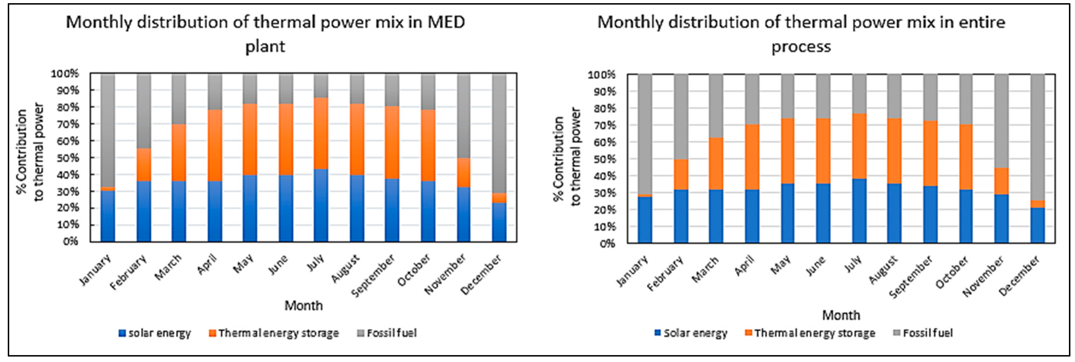
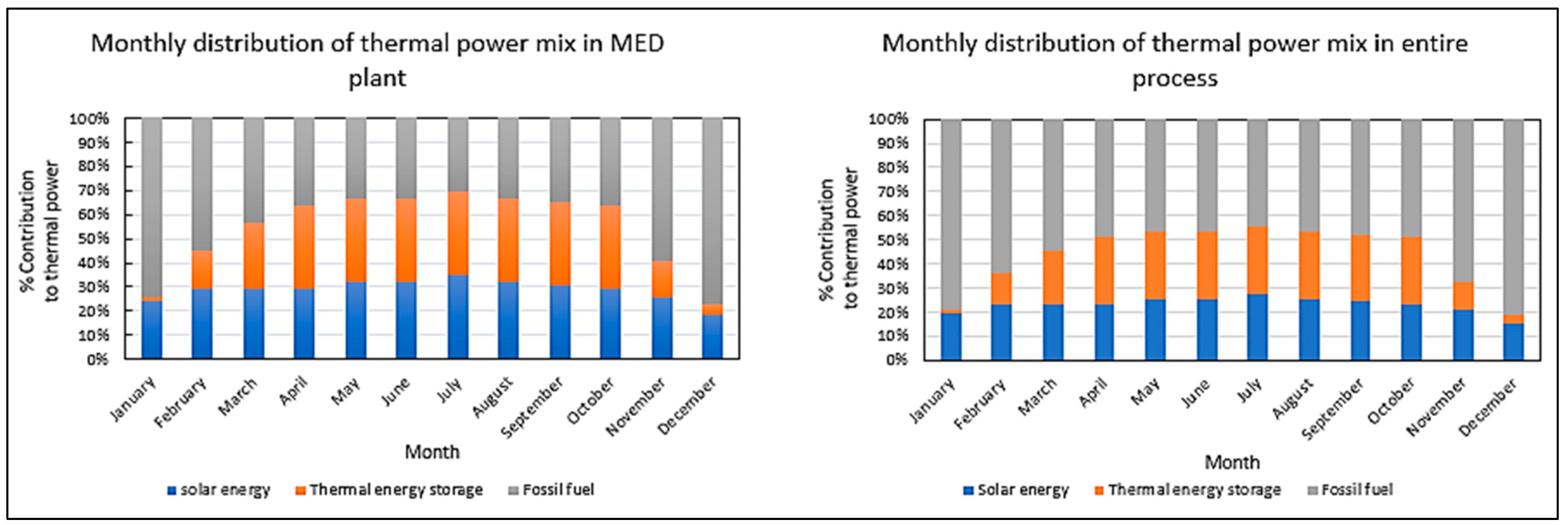
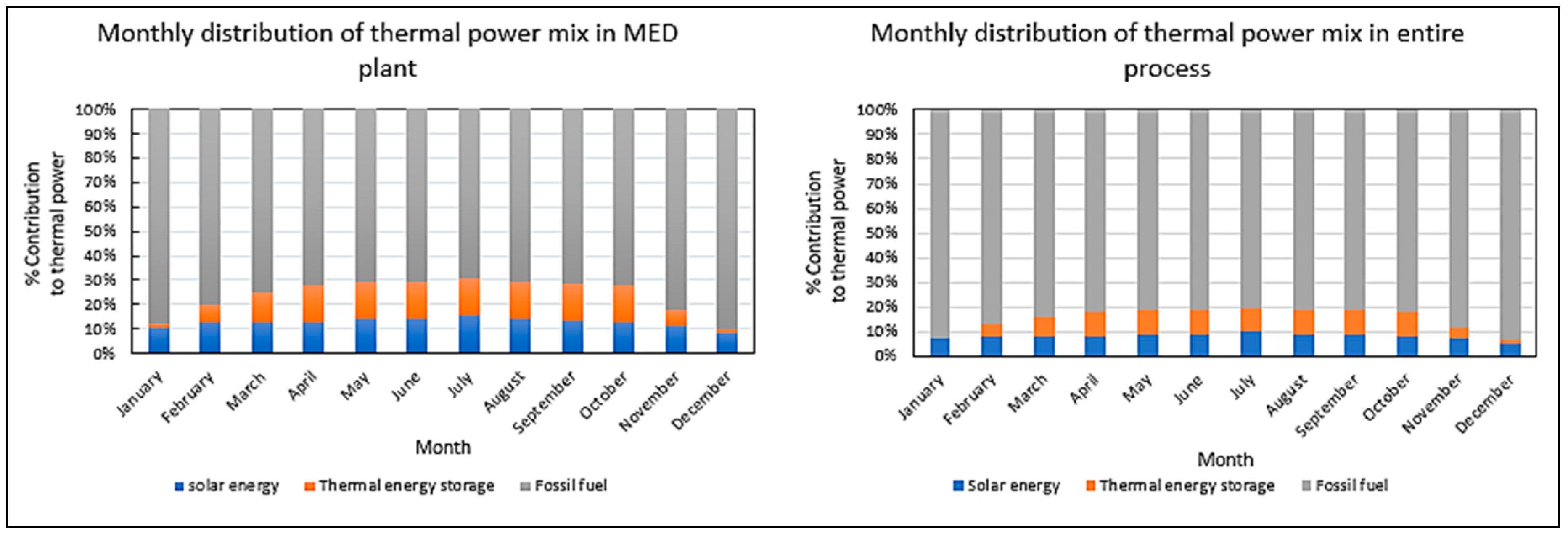
The monthly distribution of the optimal thermal power mix for the MED plant and the entire system has been determined for the different percentage contributions of RO and MED in the total desalinated water production. The optimal thermal power mix for the MED plant includes the direct thermal power of the solar field, the indirect thermal power of the thermal storage system, the surplus thermal power of the cogeneration system and the direct thermal power from the combustion of fossil fuels. The monthly distribution varies over the year due to the availability of DNI and the variability of the incident angle, as shown in Figure 4, Figure 5 and Figure 6.
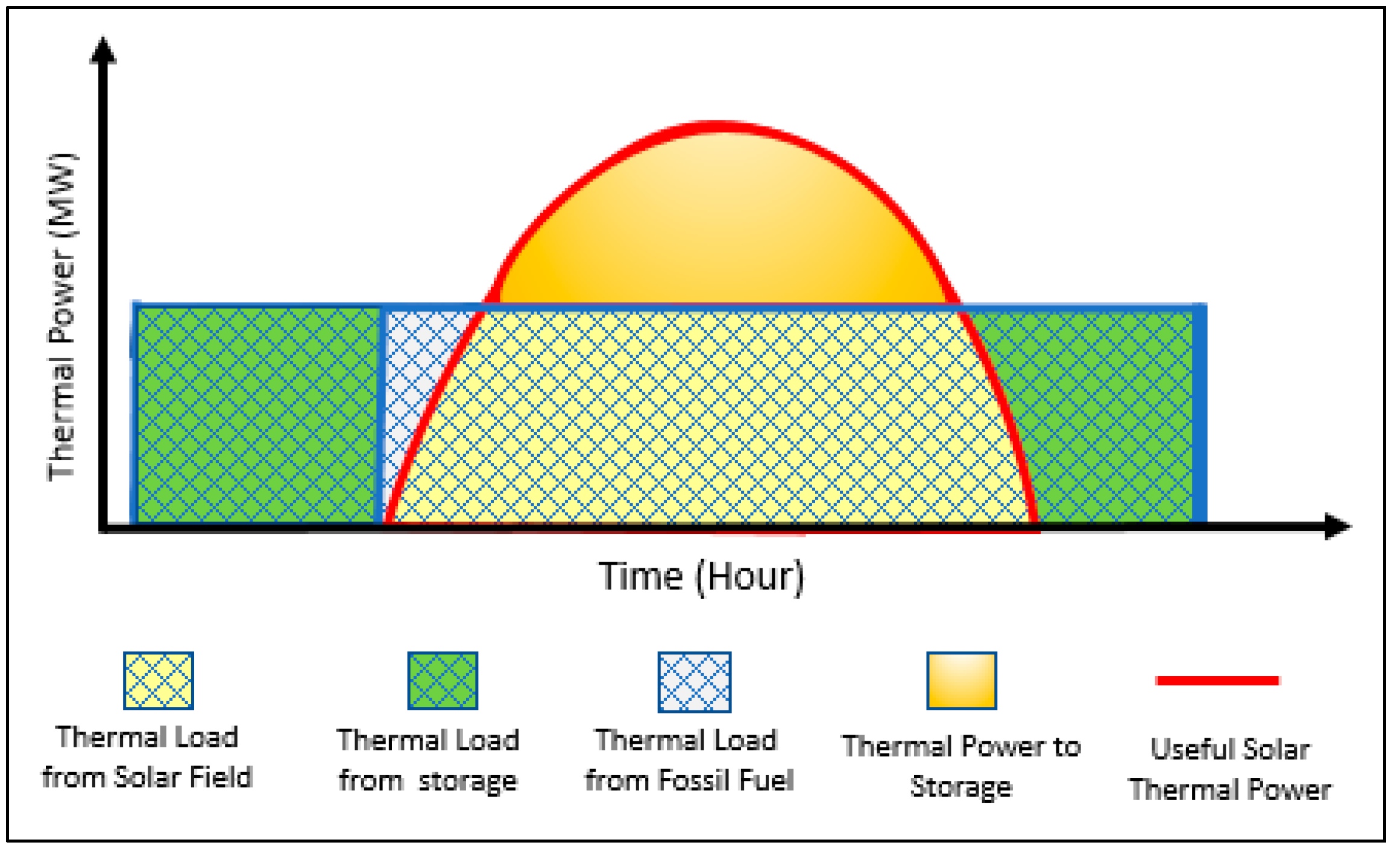
The solution of the case study introduces two scenarios to the optimal operation for MED in accordance with the availability of solar energy regardless of the percentage contribution of MED. The first scenario is for the months of January, February, November and December and shows that it favors the harnessing of direct solar thermal power during the diurnal hours and utilizing fossil fuel in the early hours of the day and in the evening. However, stored solar thermal power can be contributed from 1–2 h only because of the lack of solar energy in these months, as illustrated in Figure 7, adapted from [57].
The second scenario is for the months of April, March, May, June, July, August, December and October and shows sharply diminishing fossil fuel use up to 2 h only. Typically, direct solar thermal power is exploited in the middle of the day, while stored solar thermal power is dispatched in the early hours and in the evening, as shown in Figure 8, adapted from [43]. In future work, the previous two scenarios can be applied to the entire system in the case of integrating solar energy into cogeneration process.
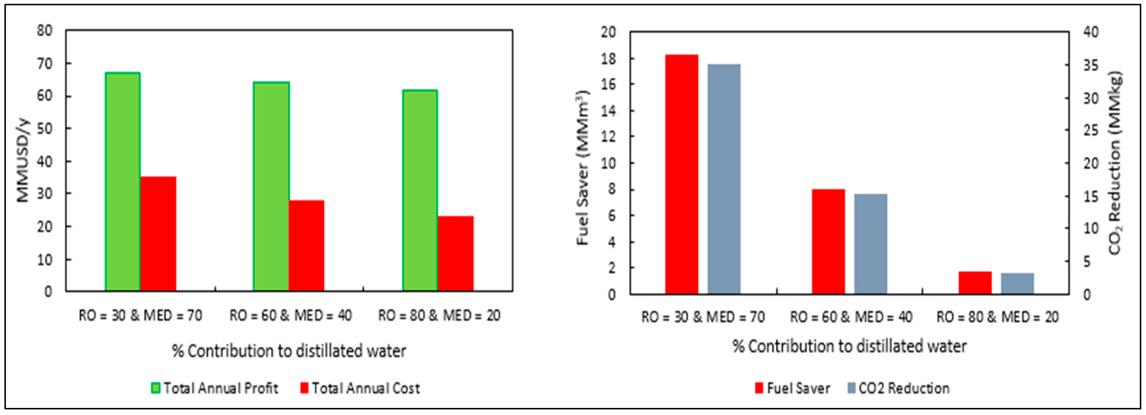
It is observed that the total annual cost of the system as mentioned in the previous section can be reduced by increasing the percentage contribution of RO over MED, but it requires consuming a great amount of fossil fuel. More consumption of fossil fuel causes serious environmental impacts due to emitting a massive amount of . From the case study, sustaining fossil fuel resources and diminishing the emissions of greenhouse gas require enhancing the percentage contribution of MED in the system based on solar energy as a provider for a high percentage of the thermal power. Figure 9 offers an obvious comparison between the economic and environmental aspects of the system through the different percentage contributions of RO and MED in the total desalinated water production. Reconciliation of economic and environmental objectives can be achieved using a sustainability weighted return on investment calculation [47,48].
The case study shows that in the Eagle Ford fields, 4.4 billion cubic feet of gas were flared in 2013, which represented around 13% of the gas in the formation [55]. Therefore, this significant amount of flared gas can be exploited as a major source of energy for the system or sharing shale gas in a specific percentage as a minor source of energy, and the results of the different percentage contribution of flared gas are shown in Table 4.
12. Conclusions
A water-energy nexus framework has been used to address water management in shale gas production. The following key elements have been integrated: solar energy, fossil fuel, cogeneration process, MED and RO. A hierarchical approach and a multi-period MINLP have been developed and solved to find the optimal mix of solar energy, thermal storage and fossil fuel and the optimal usage of water treatment technologies. A case study for Eagle Ford Basin in Texas has been solved to show the applicability of the proposed approach. The system has been analyzed according to the technical, economic and environmental aspects. The multi-period method has been applied to discretize the operational period to track the diurnal fluctuations of solar energy. The percentage utilization of water treatment technologies has been iteratively discretized. Once the solution of the mixed integer nonlinear program (MINLP) was applied to each discretization, the optimal mix of solar energy, thermal storage and fossil fuel, the optimal values of the design and operating variables of the system (e.g., minimum area of a solar collector, maximum capacity of the thermal storage system, etc.) have been determined. The results show the system’s economic and environmental merits using a water-energy nexus framework and enabling effective water management strategies while incorporating renewable energy.
Author Contributions
This paper is a collaborative research between the two authors. The general problem definition, methodology, optimization approach, and solution method were developed via discussions between the two authors. Al-Aboosi carried out the computational aspects of the optimization program and the techno-economic analysis for the case study under the supervision of El-Halwagi. Both authors contributed to writing and editing of the manuscript.
Conflicts of Interest
The authors declare no conflict of interest.
Nomenclature
| , , , | Correlation constants |
| a, b and c | Coefficients for the LS-3 collector |
| Annualized fixed capital cost of the multi-effect desalination | |
| Annualized fixed capital cost of the reverse osmosis | |
| Annualized fixed capital cost of the solar collector | |
| Annualized fixed capital cost of the cogeneration system | |
| Effective surface area of the solar collector | |
| Solar field aperture area | |
| Total annual fixed cost | |
| Total annual operating cost | |
| A and B | Parameters that depend on the type of the turbine |
| Barrel | |
| Value of avoided cost of discharging wastewater | |
| Value of fossil fuel | |
| Disposal cost per volume unit | |
| Fuel cost per thermal power unit | |
| Fresh water cost per volume unit | |
| Operation and maintenance cost per thermal power unit | |
| Primary and secondary treatment cost per volume unit | |
| Solar field cost per area unit | |
| Steam generator system cost per thermal power unit | |
| Thermal storage system cost per thermal power unit | |
| Transportation cost per volume unit | |
| Specific heat of the molten salt | |
| Specific heat of oil | |
| Outer diameter of the receiver pipe | |
| Design variable of the turbine | |
| Direct normal irradiance | |
| Electric energy requirements of MED | |
| Electric energy requirements of RO | |
| Turbine shaft power output | |
| Electric energy provided by the cogeneration turbine | |
| Cubic feet | |
| Focal length of the collectors | |
| Fixed capital cost of a boiler | |
| Fixed capital cost of the primary and secondary treatment | |
| Total fixed capital cost of the solar field | |
| Fixed capital cost estimation of the steam generator system | |
| Fixed capital cost of the turbine | |
| Fixed capital cost of the thermal storage system | |
| Total fixed capital cost | |
| Soiling factor (mirror cleanliness) | |
| Flowback and produced water | |
| Volumetric flow rate of fossil fuel | |
| Volumetric flow rate of desalinated water from MED | |
| Volumetric flow rate of desalinated water from RO | |
| Actual outlet enthalpy of the turbine | |
| Inlet enthalpy of the steam | |
| Outlet isentropic enthalpy | |
| Sum of heat collection element | |
| Incidence angle modifier | |
| Length of a single collector assembly | |
| Length of spacing between troughs | |
| Inlet turbine steam flowrate | |
| Maximum mass flowrate of the turbine | |
| Mass flow rate of molten salt | |
| Mass flowrate of oil | |
| Multi-effect distillation plant | |
| Mixed integer nonlinear program | |
| Million | |
| Factor to account for the operation pressure of the boiler | |
| Factor accounting for the superheat temperature of the boiler | |
| Service life of the property in years | |
| National Solar Radiation Data Base | |
| Operation and maintenance cost | |
| Optical end loss | |
| Cost of fuel | |
| Operation variable of the turbine | |
| Annualized operational expenditure of MED | |
| Annualized operational expenditure of RO | |
| Annualized operational expenditure of the solar collector | |
| Annualized operational expenditure of the thermal storage system | |
| Annualized operational expenditure of the cogeneration system | |
| Gauge pressure of the boiler | |
| Parabolic trough collector | |
| Thermal energy requirements of MED | |
| Thermal power output of the boiler rate | |
| Thermal power that loss from the headers (pipes) | |
| Thermal power that loss from the expansion tank (vessel) | |
| Net thermal power inside the tank | |
| Inlet thermal power | |
| Amount of thermal power that produced by the boiler | |
| Accumulated thermal power in the tank from preceding iterations | |
| Total thermal power that loss from a collector to ambient | |
| Thermal power that transferred from a collector to a fluid | |
| Thermal power that absorbed by the receiver tube of a collector loop | |
| Outlet thermal power | |
| Useful thermal power that produced by the solar field | |
| Solar thermal power that produced by the solar field | |
| Thermal power loss | |
| Direct thermal power from the solar thermal collector | |
| Direct thermal power from the combustion of fossil fuels | |
| Inlet thermal power of the thermal storage system | |
| Indirect thermal from solar energy through the thermal storage system | |
| Thermal power captured by the solar collector | |
| Loss thermal power of the thermal storage system | |
| Thermal power stored in the thermal storage system | |
| Total thermal power needs for water treatment | |
| Thermal power from steam leaving the cogeneration turbine | |
| Thermal power stored from previous iterations | |
| Row shadow loss | |
| Reverse osmosis plant | |
| Return on investment | |
| Number of storage capacity hours | |
| Cold tank temperature | |
| Hot tank temperature | |
| Superheat temperature | |
| Ambient air temperature | |
| Temperature at the inlet of the turbine | |
| Temperature of the molten salt | |
| Mean receiver pipe temperature | |
| Saturation temperature at the inlet of a turbine | |
| Overall heat transfer coefficient of the receiver pipe | |
| Width of the collector aperture | |
| Volumetric flow rate of discharging wastewater | |
| Watt |
Subscript and Superscript Symbols
| ac | Actual |
| acc | Accumulated |
| amb | Ambient |
| B | Boiler |
| c | Collector aperture |
| Cogen | Cogeneration process |
| CT | Cold tank |
| DS | Disposal |
| EL | End loss |
| f | Factor |
| F | Fuel |
| FW | Freshwater |
| g | Gauge |
| HT | Hot tank |
| is | Isentropic |
| LFP | Loss from pipes |
| LFV | Loss from vessel |
| m | Time period (month) |
| MED | Multi-effect distillation plant |
| ms | Molten salt |
| OM | Operation and maintenance |
| P | Pressure |
| PST | Primary and secondary treatment |
| rec | Receiver |
| RO | Reverse osmosis plant |
| sat | Saturation |
| SC | Solar collector |
| SCA | Single collector assembly |
| SF | Solar field |
| SG | Steam generator |
| SH | Superheat |
| SL | Shadow loss |
| t | Time period (h) |
| T | Turbine |
| TES | Thermal energy storage |
| TR | Transportation |
| w | wastewater |
Greek Symbols
| Efficiency of the boiler | |
| Isentropic efficiency of the steam turbine | |
| Annual operation time | |
| Vector set of the turbine | |
| Value of produced water from MED | |
| Value of produced water from RO | |
| For every month (operational period) | |
| For every hour (sub- period) | |
| Isentropic enthalpy change | |
| ηopt | Peak optical efficiency of a collector |
| Solar incidence angle | |
| Solar zenith angle | |
| γ | Intercept factor |
| δ | Declination |
| ΔT | Difference between inlet and outlet of the oil |
| ρ | Reflectivity |
| τ | Glass transmissivity |
| ω | Hour angle |
| Absorptivity of the receiver pipe |
Appendix A. Solar Data for the Case Study
The solar data for Eagle Ford Shale Play as extracted from National Solar Radiation Data Base (NSRDB) are shown in Table A1, Table A2, Table A3 and Table A4 to represent:
- Average hourly dry bulb temperature ()
- Average hourly wet bulb temperature ()
- Average hourly direct solar irradiance ()
- Average hourly solar incidence angle (degree).
The solar beam radiation is 500 () at the design point.

Table A1.
Average hourly dry bulb temperature ()
| Month | January | February | March | April | May | June | July | August | September | October | November | December | |
|---|---|---|---|---|---|---|---|---|---|---|---|---|---|
| Hour | |||||||||||||
| 0.5 | 7.1 | 8.1 | 13.4 | 17.3 | 20.9 | 23.6 | 13.4 | 25.1 | 24.1 | 18.9 | 13.1 | 8.2 | |
| 1.5 | 6.6 | 7.71 | 13.0 | 16.9 | 20.4 | 23.3 | 13.0 | 24.5 | 23.6 | 18.2 | 12.6 | 7.7 | |
| 2.5 | 6.1 | 7.24 | 12.6 | 16.4 | 19.9 | 23.1 | 12.6 | 24.0 | 23.2 | 17.4 | 12.3 | 7.36 | |
| 3.5 | 6.0 | 6.98 | 12.3 | 16.2 | 19.6 | 23.0 | 12.3 | 23.6 | 22.9 | 17.1 | 11.6 | 7.11 | |
| 4.5 | 5.9 | 6.74 | 12.0 | 16.0 | 19.3 | 22.8 | 12.0 | 23.2 | 22.6 | 16.8 | 11.4 | 7.13 | |
| 5.5 | 5.9 | 6.49 | 11.7 | 15.8 | 19.0 | 22.8 | 11.7 | 22.8 | 22.4 | 16.5 | 11.3 | 6.96 | |
| 6.5 | 5.5 | 7.37 | 12.6 | 16.8 | 20.1 | 23.3 | 12.6 | 24.2 | 22.4 | 17.9 | 10.9 | 7.03 | |
| 7.5 | 5.4 | 8.28 | 13.5 | 17.8 | 21.2 | 24.6 | 13.5 | 25.6 | 23.7 | 19.3 | 11.8 | 7.21 | |
| 8.5 | 7.7 | 9.20 | 14.5 | 18.8 | 22.3 | 26.0 | 14.5 | 27.0 | 25.6 | 20.6 | 14.0 | 9.10 | |
| 9.5 | 10 | 11.1 | 16.2 | 20.1 | 23.4 | 27.3 | 16.2 | 28.5 | 27.0 | 22.1 | 16.3 | 11.0 | |
| 10.5 | 12 | 13.0 | 17.9 | 21.4 | 24.5 | 28.4 | 17.9 | 30.1 | 28.2 | 23.6 | 18.0 | 12.8 | |
| 11.5 | 13 | 14.9 | 19.6 | 22.7 | 25.6 | 29.4 | 19.6 | 31.6 | 29.4 | 25.2 | 19.3 | 14.1 | |
| 12.5 | 14 | 15.7 | 20.5 | 23.5 | 26.2 | 30.4 | 20.5 | 32.4 | 30.3 | 25.8 | 20.3 | 15.1 | |
| 13.5 | 15 | 16.6 | 21.4 | 24.4 | 26.8 | 31.3 | 21.4 | 33.3 | 30.7 | 26.5 | 21.1 | 16.0 | |
| 14.5 | 15 | 17.5 | 22.3 | 25.2 | 27.5 | 31.4 | 22.3 | 34.1 | 31.0 | 27.2 | 21.3 | 16.4 | |
| 15.5 | 16 | 17.0 | 21.7 | 24.8 | 27.4 | 31.7 | 21.7 | 33.5 | 31.2 | 26.5 | 21.2 | 16.5 | |
| 16.5 | 15 | 16.5 | 21.2 | 24.4 | 27.4 | 31.2 | 21.2 | 32.9 | 31.0 | 25.8 | 20.5 | 16.0 | |
| 17.5 | 13 | 16.1 | 20.7 | 23.9 | 27.3 | 30.4 | 20.7 | 32.3 | 30.2 | 25.1 | 19.0 | 14.4 | |
| 18.5 | 12 | 14.6 | 19.1 | 22.5 | 26.1 | 29.0 | 19.1 | 30.9 | 28.8 | 24.0 | 17.3 | 12.7 | |
| 19.5 | 10.9 | 13.21 | 17.5 | 21.2 | 24.95 | 27.64 | 17.5 | 29.53 | 27.76 | 22.88 | 15.84 | 11.2 | |
| 20.5 | 9.73 | 11.77 | 16.0 | 19.8 | 23.7 | 26.47 | 16.0 | 28.10 | 26.68 | 21.75 | 14.63 | 10.3 | |
| 21.5 | 8.63 | 10.79 | 15.3 | 19.2 | 23.0 | 25.44 | 15.3 | 27.30 | 25.93 | 21.00 | 13.95 | 9.77 | |
| 22.5 | 7.91 | 9.825 | 14.5 | 18.5 | 22.3 | 24.75 | 14.5 | 26.46 | 25.36 | 20.25 | 13.45 | 9.55 | |
| 23.5 | 7.56 | 8.846 | 13.8 | 17.7 | 21.5 | 24.0 | 13.8 | 25.6 | 24.7 | 19.6 | 13.30 | 9.31 | |
Table A2.
Average hourly wet bulb temperature (°C).
| Month | January | February | March | April | May | June | July | August | September | October | November | December | |
|---|---|---|---|---|---|---|---|---|---|---|---|---|---|
| Hour | |||||||||||||
| 0.5 | 5.7 | 6.3 | 9.85 | 15.3 | 18.5 | 21.6 | 22.9 | 22.0 | 21.5 | 16.3 | 11.4 | 6.41 | |
| 1.5 | 5.4 | 6.0 | 9.69 | 15.1 | 18.3 | 21.5 | 22.8 | 22.0 | 21.3 | 15.9 | 11.1 | 6.03 | |
| 2.5 | 4.9 | 5.7 | 9.52 | 14.9 | 18.0 | 21.4 | 22.7 | 21.9 | 21.2 | 15.4 | 10.8 | 5.75 | |
| 3.5 | 4.9 | 5.5 | 9.43 | 14.7 | 17.8 | 21.4 | 22.7 | 21.8 | 21.0 | 15.1 | 10.2 | 5.55 | |
| 4.5 | 4.8 | 5.3 | 9.35 | 14.6 | 17.6 | 21.4 | 22.6 | 21.6 | 20.9 | 14.9 | 10.1 | 5.56 | |
| 5.5 | 4.8 | 5.0 | 9.21 | 14.5 | 17.4 | 21.4 | 22.6 | 21.4 | 20.8 | 14.6 | 10.0 | 5.40 | |
| 6.5 | 4.5 | 5.7 | 9.64 | 15.1 | 18.1 | 21.7 | 22.9 | 22.0 | 20.8 | 15.6 | 9.78 | 5.44 | |
| 7.5 | 4.3 | 6.3 | 10.0 | 15.7 | 18.8 | 22.2 | 23.3 | 22.6 | 21.4 | 16.4 | 10.3 | 5.60 | |
| 8.5 | 6.1 | 7.0 | 10.4 | 16.3 | 19.4 | 22.6 | 23.4 | 23.1 | 22.0 | 17.2 | 11.6 | 6.99 | |
| 9.5 | 7.5 | 8.0 | 11.3 | 17.0 | 19.8 | 22.7 | 23.6 | 23.4 | 22.2 | 17.8 | 12.7 | 8.08 | |
| 10.5 | 8.4 | 8.9 | 12.0 | 17.6 | 20.1 | 22.8 | 23.6 | 23.4 | 22.2 | 18.3 | 13.3 | 8.90 | |
| 11.5 | 9.1 | 9.6 | 12.5 | 18.1 | 20.4 | 23.0 | 23.5 | 23.3 | 22.1 | 18.7 | 13.8 | 9.42 | |
| 12.5 | 9.5 | 10 | 12.7 | 18.4 | 20.7 | 23.0 | 23.5 | 23.3 | 22.3 | 18.8 | 14.0 | 9.82 | |
| 13.5 | 10 | 10 | 12.9 | 18.6 | 21.0 | 23.2 | 23.5 | 23.2 | 22.2 | 18.9 | 14.2 | 10.1 | |
| 14.5 | 10 | 10 | 13.0 | 18.8 | 21.2 | 22.9 | 23.5 | 23.0 | 22.1 | 19.0 | 14.1 | 10.3 | |
| 15.5 | 10 | 10 | 12.8 | 18.5 | 21.1 | 22.9 | 23.4 | 22.8 | 22.0 | 18.7 | 14.1 | 10.2 | |
| 16.5 | 9.8 | 10 | 12.5 | 18.3 | 20.9 | 22.8 | 23.3 | 22.6 | 22.0 | 18.5 | 13.8 | 10.0 | |
| 17.5 | 9.2 | 9.8 | 12.2 | 18.1 | 20.7 | 22.7 | 23.3 | 22.3 | 22.0 | 18.2 | 13.3 | 9.39 | |
| 18.5 | 8.6 | 9.4 | 11.9 | 17.6 | 20.5 | 22.4 | 23.4 | 22.4 | 21.8 | 18.0 | 12.7 | 8.72 | |
| 19.5 | 8.0 | 8.9 | 11.4 | 17.1 | 20.2 | 22.3 | 23.4 | 22.4 | 21.8 | 17.7 | 12.2 | 8.13 | |
| 20.5 | 7.4 | 8.3 | 10.8 | 16.5 | 19.8 | 22.1 | 23.2 | 22.1 | 21.6 | 17.3 | 11.7 | 7.78 | |
| 21.5 | 6.9 | 7.9 | 10.6 | 16.3 | 19.5 | 22.0 | 23.2 | 22.2 | 21.6 | 17.1 | 11.4 | 7.50 | |
| 22.5 | 6.4 | 7.4 | 10.3 | 16.0 | 19.2 | 21.9 | 23.1 | 22.1 | 21.6 | 16.9 | 11.3 | 7.37 | |
| 23.5 | 6.1 | 6.8 | 9.91 | 15.5 | 18.7 | 21.7 | 22.9 | 21.9 | 21.6 | 16.7 | 11.4 | 7.30 | |
Table A3.
Average hourly direct solar irradiance ()
| Month | January | February | March | April | May | June | July | August | September | October | November | December | |
|---|---|---|---|---|---|---|---|---|---|---|---|---|---|
| Hour | |||||||||||||
| 0.5 | 0 | 0 | 0 | 0 | 0 | 0 | 0 | 0 | 0 | 0 | 0 | 0 | |
| 1.5 | 0 | 0 | 0 | 0 | 0 | 0 | 0 | 0 | 0 | 0 | 0 | 0 | |
| 2.5 | 0 | 0 | 0 | 0 | 0 | 0 | 0 | 0 | 0 | 0 | 0 | 0 | |
| 3.5 | 0 | 0 | 0 | 0 | 0 | 0 | 0 | 0 | 0 | 0 | 0 | 0 | |
| 4.5 | 0 | 0 | 0 | 0 | 0 | 0 | 0 | 0 | 0 | 0 | 0 | 0 | |
| 5.5 | 0 | 0 | 0 | 0 | 5.1 | 3.8 | 1 | 0.0 | 0 | 0 | 0 | 0 | |
| 6.5 | 0 | 0 | 9.6 | 26 | 109 | 86 | 65 | 57 | 34 | 26 | 1.8 | 0 | |
| 7.5 | 48 | 95 | 140 | 145 | 216 | 164 | 236 | 229 | 184 | 221 | 171 | 49 | |
| 8.5 | 240 | 244 | 287 | 228 | 258 | 319 | 350 | 347 | 315 | 337 | 328 | 199 | |
| 9.5 | 339 | 346 | 365 | 281 | 318 | 377 | 467 | 463 | 450 | 460 | 388 | 272 | |
| 10.5 | 396 | 413 | 413 | 352 | 362 | 470 | 550 | 524 | 516 | 497 | 462 | 359 | |
| 11.5 | 415 | 487 | 478 | 394 | 383 | 496 | 630 | 573 | 557 | 553 | 545 | 389 | |
| 12.5 | 473 | 468 | 498 | 439 | 462 | 526 | 621 | 599 | 569 | 566 | 544 | 459 | |
| 13.5 | 457 | 474 | 481 | 461 | 460 | 545 | 603 | 600 | 521 | 542 | 504 | 489 | |
| 14.5 | 415 | 440 | 417 | 467 | 445 | 520 | 576 | 540 | 540 | 544 | 481 | 499 | |
| 15.5 | 397 | 433 | 380 | 473 | 503 | 489 | 529 | 539 | 493 | 498 | 437 | 440 | |
| 16.5 | 283 | 365 | 323 | 414 | 434 | 475 | 536 | 417 | 422 | 401 | 361 | 323 | |
| 17.5 | 128 | 246 | 234 | 338 | 356 | 389 | 427 | 323 | 311 | 181 | 93 | 80 | |
| 18.5 | 0.4 | 32 | 54 | 119 | 166 | 217 | 234 | 140 | 53 | 3.6 | 0 | 0 | |
| 19.5 | 0 | 0 | 0 | 0.1 | 7.2 | 21 | 24 | 4.3 | 0 | 0 | 0 | 0 | |
| 20.5 | 0 | 0 | 0 | 0 | 0 | 0 | 0 | 0 | 0 | 0 | 0 | 0 | |
| 21.5 | 0 | 0 | 0 | 0 | 0 | 0 | 0 | 0 | 0 | 0 | 0 | 0 | |
| 22.5 | 0 | 0 | 0 | 0 | 0 | 0 | 0 | 0 | 0 | 0 | 0 | 0 | |
| 23.5 | 0 | 0 | 0 | 0 | 0 | 0 | 0 | 0 | 0 | 0 | 0 | 0 | |
Table A4.
Average hourly solar incidence angle (degree).
| Month | January | February | March | April | May | June | July | August | September | October | November | December | |
|---|---|---|---|---|---|---|---|---|---|---|---|---|---|
| Hour | |||||||||||||
| 0.5 | 0 | 0 | 0 | 0 | 0 | 0 | 0 | 0 | 0 | 0 | 0 | 0 | |
| 1.5 | 0 | 0 | 0 | 0 | 0 | 0 | 0 | 0 | 0 | 0 | 0 | 0 | |
| 2.5 | 0 | 0 | 0 | 0 | 0 | 0 | 0 | 0 | 0 | 0 | 0 | 0 | |
| 3.5 | 0 | 0 | 0 | 0 | 0 | 0 | 0 | 0 | 0 | 0 | 0 | 0 | |
| 4.5 | 0 | 0 | 0 | 0 | 0 | 0 | 0 | 0 | 0 | 0 | 0 | 0 | |
| 5.5 | 0 | 0 | 0 | 0 | 0 | 0 | 0 | 0 | 0 | 0 | 0 | 0 | |
| 6.5 | 0 | 0 | 0 | 6.04 | 16.1 | 20.2 | 19.2 | 11.1 | 0 | 0 | 0 | 0 | |
| 7.5 | 0 | 4.33 | 7.10 | 2.51 | 9.26 | 13.4 | 12.3 | 5.49 | 4.95 | 16.1 | 23.4 | 0 | |
| 8.5 | 30.6 | 23.6 | 14.3 | 4.99 | 2.85 | 6.99 | 5.77 | 2.49 | 11.8 | 23.4 | 31.8 | 34.4 | |
| 9.5 | 37.8 | 30.5 | 20.7 | 10.9 | 2.76 | 1.52 | 1.14 | 7.13 | 18.0 | 29.8 | 38.5 | 41.4 | |
| 10.5 | 43.8 | 36.3 | 26.1 | 15.6 | 7.01 | 2.69 | 4.28 | 11.8 | 22.9 | 35.0 | 44.0 | 47.1 | |
| 11.5 | 48.2 | 40.6 | 30.0 | 18.7 | 9.73 | 5.40 | 7.20 | 14.9 | 26.3 | 38.4 | 47.6 | 51.1 | |
| 12.5 | 50.2 | 42.7 | 31.8 | 20.0 | 10.7 | 6.44 | 8.40 | 16.2 | 27.5 | 39.3 | 48.5 | 52.6 | |
| 13.5 | 49.5 | 42.1 | 31.0 | 19.0 | 9.79 | 5.70 | 7.78 | 15.3 | 26.2 | 37.5 | 46.5 | 51.1 | |
| 14.5 | 46.1 | 39.0 | 27.8 | 16.0 | 7.06 | 3.20 | 5.40 | 12.7 | 22.8 | 33.4 | 42.2 | 47.2 | |
| 15.5 | 40.7 | 34.0 | 22.9 | 11.5 | 2.79 | 0.83 | 1.58 | 8.49 | 17.8 | 27.8 | 36.2 | 41.4 | |
| 16.5 | 34.0 | 27.7 | 16.9 | 5.74 | 2.83 | 6.15 | 3.82 | 3.07 | 11.7 | 21.1 | 29.2 | 34.4 | |
| 17.5 | 21.1 | 20.4 | 9.96 | 2.65 | 9.23 | 12.4 | 10.1 | 3.61 | 4.78 | 11.5 | 0 | 0 | |
| 18.5 | 0 | 0 | 0.17 | 8.06 | 16.1 | 19.2 | 16.9 | 10.5 | 0.99 | 0 | 0 | 0 | |
| 19.5 | 0 | 0 | 0 | 0 | 0 | 0 | 0 | 0 | 0 | 0 | 0 | 0 | |
| 20.5 | 0 | 0 | 0 | 0 | 0 | 0 | 0 | 0 | 0 | 0 | 0 | 0 | |
| 21.5 | 0 | 0 | 0 | 0 | 0 | 0 | 0 | 0 | 0 | 0 | 0 | 0 | |
| 22.5 | 0 | 0 | 0 | 0 | 0 | 0 | 0 | 0 | 0 | 0 | 0 | 0 | |
| 23.5 | 0 | 0 | 0 | 0 | 0 | 0 | 0 | 0 | 0 | 0 | 0 | 0 | |
References
- Zhang, C.; El-Halwagi, M.M. Estimate the Capital Cost of Shale-Gas Monetization Projects. Chem. Eng. Prog. 2017, 113, 28–32. [Google Scholar]
- Al-Douri, A.; Sengupta, D.; El-Halwagi, M.M. Shale Gas Monetization—A Review of Downstream Processing to Chemicals and Fuels. J. Nat. Gas Sci. Eng. 2017, 45, 436–455. [Google Scholar]
- Ortiz-Espinoza, P.A.; Jiménez-Gutiérreza, A.; Nourledin, M.; El-Halwagi, M.M. Design, Simulation and Techno-Economic Analysis of Two Processes for the Conversion of Shale Gas to Ethylene. Comp. Chem. Eng. 2017, 107, 237–246. [Google Scholar] [CrossRef]
- Pérez-Uresti, S.I.; Adrián-Mendiola, J.M.; El-Halwagi, M.M.; Jiménez-Gutiérrez, A. Techno-Economic Assessment of Benzene Production from Shale Gas. Processes 2017, 5, 33. [Google Scholar] [CrossRef]
- Jasper, S.; El-Halwagi, M.M. A Techno-Economic Comparison of Two Methanol-to-Propylene Processes. Processes 2015, 3, 684–698. [Google Scholar] [CrossRef]
- Julián-Durán, L.; Ortiz-Espinoza, A.P.; El-Halwagi, M.M.; Jiménez-Gutiérrez, A. Techno-economic assessment and environmental impact of shale gas alternatives to methanol. ACS Sustain. Chem. Eng. 2014, 2, 2338–2344. [Google Scholar] [CrossRef]
- Salkuyeh, Y.K.; Adams, T.A., II. A novel polygeneration process to co-produce ethylene and electricity from shale gas with zero CO2 emissions via methane oxidative coupling. Energy Convers. Manag. 2015, 92, 406–420. [Google Scholar] [CrossRef]
- Ehlinger, M.V.; Gabriel, K.J.; Noureldin, M.M.B.; El-Halwagi, M.M. Process Design and Integration of Shale Gas to Methanol. ACS Sustain. Chem. Eng. 2014, 2, 30–37. [Google Scholar] [CrossRef]
- Salkuyeh, Y.K.; Adams, T.A., II. Shale gas for the petrochemical industry: Incorporation of novel technologies. In Computer Aided Chemical Engineering; Elsevier: New York, NY, USA, 2014; Volume 34, pp. 603–608. [Google Scholar]
- Hasaneen, R.; El-Halwagi, M.M. Integrated Process and Microeconomic Analyses to Enable Effective Environmental Policy for Shale Gas in the United States. Clean Technol. Environ. Policy 2017, 19, 1775–1789. [Google Scholar] [CrossRef]
- Arredondo-Ramírez, K.; Ponce-Ortega, J.M.; El-Halwagi, M.M. Optimal Planning and Infrastructure Development of Shale Gas. Energy Convers. Manag. 2016, 119, 91–100. [Google Scholar] [CrossRef]
- Gao, J.; You, F. Optimal design and operations of supply chain networks for water management in shale gas production: MILFP model and algorithms for the water-energy nexus. AIChE J. 2015, 61, 1184–1208. [Google Scholar] [CrossRef]
- Carrero-Parreño, A.; Onishi, V.C.; Salcedo-Díaz, R.; Ruiz-Femenia, R.; Fraga, E.S.; Caballero, J.A.; Reyes-Labarta, J.A. Optimal Pretreatment System of Flowback Water from Shale Gas Production. Ind. Eng. Chem. Res. 2017, 56, 4386–4398. [Google Scholar] [CrossRef]
- Yang, L.; Grossmann, I.E.; Manno, J. Optimization models for shale gas water management. AIChE J. 2014, 60, 3490–3501. [Google Scholar] [CrossRef]
- Nicot, J.-P.; Scanlon, B.R. Water Use for Shale-Gas Production in Texas. U.S. Environ. Sci. Technol. 2012, 46, 3580–3586. [Google Scholar] [CrossRef] [PubMed]
- Elsayed, A.N.; Barrufet, M.A.; Eljack, F.T.; El-Halwagi, M.M. Optimal Design of Thermal Membrane Distillation Systems for the Treatment of Shale Gas Flowback Water. Int. J. Membr. Sci. Technol. 2015, 2, 1–9. [Google Scholar]
- Boschee, P. Produced and Flowback Water Recycling and Reuse: Economics, Limitations, and Technology. Oil Gas Facil. 2014, 3, 16–21. [Google Scholar] [CrossRef]
- Lira-Barragán, L.; Ponce-Ortega, J.M.; Guillén-Gosálbez, G.; El-Halwagi, M.M. Optimal Water Management under Uncertainty for Shale Gas Production. Ind. Eng. Chem. Res. 2016, 55, 1322–1335. [Google Scholar] [CrossRef]
- Chen, H.; Carter, K.E. Water usage for natural gas production through hydraulic fracturing in the United States from 2008 to 2014. J. Environ. Manag. 2016, 170, 152–159. [Google Scholar] [CrossRef] [PubMed]
- Shaffer, D.L.; Chavez, L.H.A.; Ben-Sasson, M.; Castrillón, S.R.; Yip, N.Y.; Elimelech, M. Desalination and reuse of high-salinity shale gas produced water: Drivers, technologies, and future directions. Environ. Sci. Technol. 2013, 47, 9569–9583. [Google Scholar] [CrossRef] [PubMed]
- Lokare, O.R.; Tavakkoli, S.; Rodriguez, G.; Khanna, V.; Vidic, R.D. Integrating membrane distillation with waste heat from natural gas compressor stations for produced water treatment in Pennsylvania. Desalination 2017, 413, 144–153. [Google Scholar] [CrossRef]
- Tavakkoli, S.; Lokare, O.R.; Vidic, R.D.; Khanna, V. A techno-economic assessment of membrane distillation for treatment of Marcellus shale produced water. Desalination 2017, 416, 24–34. [Google Scholar] [CrossRef]
- Bamufleh, H.; Abdelhady, F.; Baaqeel, H.M.; El-Halwagi, M.M. Optimization of Multi-Effect Distillation with Brine Treatment via Membrane Distillation and Process Heat Integration. Desalination 2017, 408, 110–118. [Google Scholar] [CrossRef]
- Gabriel, K.; El-Halwagi, M.M.; Linke, P. Optimization Across Water-Energy Nexus for Integrating Heat, Power, and Water for Industrial Processes Coupled with Hybrid Thermal-Membrane Desalination. Ind. Eng. Chem. Res. 2016, 55, 3442–3466. [Google Scholar] [CrossRef]
- Elsayed, A.N.; Barrufet, M.A.; El-Halwagi, M.M. An Integrated Approach for Incorporating Thermal Membrane Distillation in Treating Water in Heavy Oil Recovery using SAGD. J. Unconv. Oil Gas Resour. 2015, 12, 6–14. [Google Scholar] [CrossRef]
- González-Bravo, R.; Nápoles-Rivera, F.; Ponce-Ortega, J.M.; Nyapathi, M.; Elsayed, N.A.; El-Halwagi, M.M. Synthesis of Optimal Thermal Membrane Distillation Networks. AIChE J. 2015, 61, 448–463. [Google Scholar] [CrossRef]
- González-Bravo, R.; Elsayed, N.A.; Ponce-Ortega, J.M.; Nápoles-Rivera, F.; Serna-González, M.; El-Halwagi, M.M. Optimal Design of Thermal Membrane Distillation Systems with Heat Integration with Process Plants. Appl. Therm. Eng. 2014, 75, 154–166. [Google Scholar] [CrossRef]
- Elsayed, A.N.; Barrufet, M.A.; El-Halwagi, M.M. Integration of Thermal Membrane Distillation Networks with Processing Facilities. Ind. Eng. Chem. Res. 2014, 53, 5284–5298. [Google Scholar] [CrossRef]
- Tovar-Facio, J.; Eljack, F.; Ponce-Ortega, J.M.; El-Halwagi, M.M. Optimal Design of Multiplant Cogeneration Systems with Uncertain Flaring and Venting. ACS Sustain. Chem. Eng. 2016, 5, 675–688. [Google Scholar] [CrossRef]
- Pham, V.; Laird, C.; El-Halwagi, M.M. Convex Hull Discretization Approach to the Global Optimization of Pooling Problems. Ind. Eng. Chem. Res. 2009, 48, 1973–1979. [Google Scholar] [CrossRef]
- Gabriel, F.; El-Halwagi, M.M. Simultaneous Synthesis of Waste Interception and Material Reuse Networks: Problem Reformulation for Global Optimization. Environ. Prog. 2005, 24, 171–180. [Google Scholar] [CrossRef]
- El-Halwagi, M.M. Sustainable Design through Process Integration: Fundamentals and Applications to Industrial Pollution Prevention, Resource Conservation, and Profitability Enhancement, 2nd ed.; IChemE/Elsevier: New York, NY, USA, 2017. [Google Scholar]
- Khor, S.C.; Foo, D.C.Y.; El-Halwagi, M.M.; Tan, R.R.; Shah, N. A Superstructure Optimization Approach for Membrane Separation-Based Water Regeneration Network Synthesis with Detailed Nonlinear Mechanistic Reverse Osmosis Model. Ind. Eng. Chem. Res. 2011, 50, 13444–13456. [Google Scholar] [CrossRef]
- Alnouri, S.; Linke, P.; El-Halwagi, M.M. Synthesis of Industrial Park Water Reuse Networks Considering Treatment Systems and Merged Connectivity Options. Comp. Chem. Eng. 2016, 91, 289–306. [Google Scholar] [CrossRef]
- El-Halwagi, M.A.; Manousiouthakis, V.; El-Halwagi, M.M. Analysis and Simulation of Hollwo Fiber Reverse Osmosis Modules. Sep. Sci. Technol. 1996, 31, 2505–2529. [Google Scholar] [CrossRef]
- El-Halwagi, M.M. Synthesis of Optimal Reverse-Osmosis Networks for Waste Reduction. AIChE J. 1992, 38, 1185–1198. [Google Scholar] [CrossRef]
- Goswami, D.Y.; Kreith, F. Energy Conversion; CRC Press: Boca Raton, FL, USA, 2007. [Google Scholar]
- Mittelman, G.; Epstein, M. A novel power block for CSP systems. Sol. Energy 2010, 84, 1761–1771. [Google Scholar] [CrossRef]
- Eck, M.; Hirsch, T.; Feldhoff, J.F.; Kretschmann, D.; Dersch, J.; Morales, A.G.; Gonzalez-Martinez, L.; Bachelier, C.; Platzer, W.; Riffelmann, K.-J. Guidelines for CSP yield analysis–optical losses of line focusing systems; definitions, sensitivity analysis and modeling approaches. Energy Procedia 2014, 49, 1318–1327. [Google Scholar] [CrossRef]
- Channiwala, S.; Ekbote, A. A generalized model to estimate field size for solar-only parabolic trough plant. In Proceedings of the 3rd Southern African Solar Energy Conference, Skukuza, South Africa, 11–13 May 2015. [Google Scholar]
- Lovegrove, K.; Stein, W. Concentrating Solar Power Technology: Principles, Developments and Applications; Elsevier: New York, NY, USA, 2012. [Google Scholar]
- Quaschning, V.; Kistner, R.; Ortmanns, W. Influence of direct normal irradiance variation on the optimal parabolic trough field size: A problem solved with technical and economical simulations. J. Sol. Energy Eng. 2002, 124, 160–164. [Google Scholar] [CrossRef]
- Herrmann, U.; Kearney, D.W. Survey of thermal energy storage for parabolic trough power plants. J. Sol. Energy Eng. 2002, 124, 145–152. [Google Scholar] [CrossRef]
- Al-Azri, N.; Al-Thubaiti, M.; El-Halwagi, M.M. An Algorithmic Approach to the Optimization of Process Cogeneration. J. Clean Technol. Environ. Policy 2009, 11, 329–338. [Google Scholar] [CrossRef]
- Mavromatis, S.; Kokossis, A. Conceptual optimisation of utility networks for operational variations—I. Targets and level optimisation. Chem. Eng. Sci. 1998, 53, 1585–1608. [Google Scholar] [CrossRef]
- Bamufleh, S.H.; Ponce-Ortega, J.M.; El-Halwagi, M.M. Multi-objective optimization of process cogeneration systems with economic, environmental, and social tradeoffs. Clean Technol. Environ. Policy 2013, 15, 185–197. [Google Scholar] [CrossRef]
- El-Halwagi, M.M. A Return on Investment Metric for Incorporating Sustainability in Process Integration and Improvement Projects. Clean Technol. Environ. Policy 2017, 19, 611–617. [Google Scholar] [CrossRef]
- Guillen-Cuevas, K.; Ortiz-Espinoza, A.P.; Ozinan, E.; Jiménez-Gutiérrez, A.; Kazantzis, N.K.; El-Halwagi, M.M. Incorporation of Safety and Sustainability in Conceptual Design via A Return on Investment Metric. ACS Sustain. Chem. Eng. 2018, 6, 1411–1416. [Google Scholar] [CrossRef]
- Kondash, J.A.; Albright, E.; Vengosh, A. Quantity of flowback and produced waters from unconventional oil and gas exploration. Sci. Total Environ. 2017, 574, 314–321. [Google Scholar] [CrossRef] [PubMed]
- Atilhan, S.; Linke, P.; Abdel-Wahab, A.; El-Halwagi, M.M. A Systems Integration Approach to the Design of Regional Water Desalination and Supply Networks. Int. J. Process Syst. Eng. 2011, 1, 125–135. [Google Scholar] [CrossRef]
- Ghaffour, N.; Missimer, T.M.; Amy, G.L. Technical review and evaluation of the economics of water desalination: Current and future challenges for better water supply sustainability. Desalination 2013, 309, 197–207. [Google Scholar] [CrossRef]
- Mezher, T.; Fath, H.; Abbas, Z.; Khaled, A. Techno-economic assessment and environmental impacts of desalination technologies. Desalination 2011, 266, 263–273. [Google Scholar] [CrossRef]
- National Renewable Energy Laboratory. Assessment of Parabolic Trough and Power Tower Solar Technology Cost and Performance Forecasts; DIANE Publishing: Collingdale, PA, USA, 2003. [Google Scholar]
- Price, H. A parabolic trough solar power plant simulation model. In Proceedings of the ASME International Solar Energy Conference, Kohala Coast, HI, USA, 15–18 March 2003. [Google Scholar]
- Horwitt, D.; Sumi, L. Up in Flames: US Shale Oil Boom Comes at Expense of Wasted Natural Gas, Increased CO2; Earthworks: Washington, DC, USA, 2014. [Google Scholar]
- RPSEA. Advanced Treatment of Shale Gas Fracturing Water to Produce Re-Use or Discharge Quality Water. 2015. Retrieved November, 2017. Available online: https://www.rpsea.org/node/222 (accessed on 18 Novemeber 2017).
- Giuliano, S.; Buck, R.; Eguiguren, S. Analysis of solar-thermal power plants with thermal energy storage and solar-hybrid operation strategy. J. Sol. Energy Eng. 2011, 133, 031007. [Google Scholar] [CrossRef]
Figure 1.
Proposed superstructure representation.

Figure 2.
Proposed approach.

Figure 3.
Monthly average of hourly direct normal irradiance (DNI) and useful thermal power.


Figure 4.
Optimal thermal power mix for MED plant and the entire system with 30% RO 70% MED.

Figure 5.
Optimal thermal power mix for the MED plant and the entire system with 60% RO 40% MED.

Figure 6.
Optimal thermal power mix for the MED plant and the entire system with 80% RO 20% MED.

Figure 7.
Optimal operation for MED during January, February, November and December.
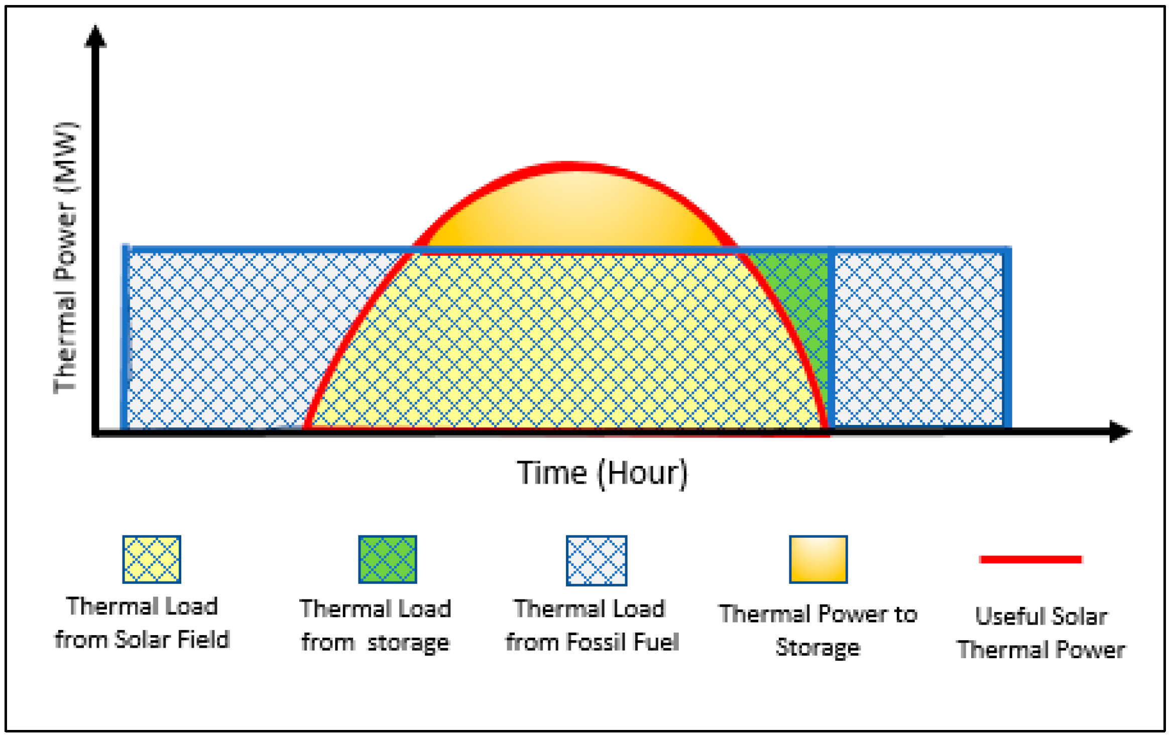
Figure 8.
Optimal operation for MED during April, March, May, June, July, August, December and October.
Figure 8.
Optimal operation for MED during April, March, May, June, July, August, December and October.

Figure 9.
Comparison between the economic and environmental aspects.

| Technology | Thermal Energy Consumption (kWht/m3 Desalinated Water) | Electric Energy Consumption (kWhe/m3 Desalinated Water) | Annualized Fixed Cost (AFC) ($/year) | Operating Cost ($/m3 seawater) | Water Recovery (m3 Desalinated Water/m3 Feed Seawater) | Value of Desalinated Water ($/m3 Desalinated Water) | Outlet Salt Content (ppm) |
|---|---|---|---|---|---|---|---|
| RO | - | 4 | 0.18 | 0.55 | 0.88 | 200 | |
| MED | 65 | 2 | 0.24 | 0.65 | 0.82 | 80 |
| Item | Receivers | Mirrors | Concentrator Structure | Concentrator Erection | Drive | Piping |
| Cost $/m2 | 43 | 40 | 47 | 14 | 13 | 10 |
| Item | Electronic and Control | Header Piping | Civil Works | Spares, HTF, Freight | Contingency | Structures and Improvement |
| Cost $/m2 | 14 | 7 | 18 | 17 | 11 | 7 |
Table 3.
Cost of transportation, fresh water, treatment and disposal of FPW.
| Type | ($/barrel) |
|---|---|
| Fresh water | 0.24 |
| Disposal (deep well + landfill) | 0.05 |
| Primary and secondary treatment | 0.34 |
| Transportation | 0.89 |
Table 4.
Technical and economic results for the system.
| Percentage Contribution * (%) | Percentage Contribution ** (%) | Total Annual Cost (MM $/year) | Annual Net (After Tax) Profit (MM $/year) | ROI (%) | Payback Period (year) |
|---|---|---|---|---|---|
| 0.0 | 35.3 | 50.4 | 14.9 | 5.9 | |
| 50 | 35.1 | 50.6 | 14.96 | 5.6 | |
| 100 | 34.8 | 50.8 | 15 | 5.5 | |
| 0.0 | 28.1 | 48.8 | 17.2 | 4.9 | |
| 50 | 27.8 | 49 | 17 | 4.8 | |
| 100 | 27.5 | 49.2 | 17.3 | 4.8 | |
| 0.0 | 23.5 | 47.7 | 19.1 | 4.4 | |
| 50 | 23.2 | 47.9 | 19.2 | 4.3 | |
| 100 | 22.8 | 48.1 | 19.3 | 4.3 |
* The percentage contribution of RO and MED plants in the total desalinated water production; ** the percentage contribution of flared gas as a source of energy.
© 2018 by the authors. Licensee MDPI, Basel, Switzerland. This article is an open access article distributed under the terms and conditions of the Creative Commons Attribution (CC BY) license (http://creativecommons.org/licenses/by/4.0/).
Share and Cite
MDPI and ACS Style
Al-Aboosi, F.Y.; El-Halwagi, M.M. An Integrated Approach to Water-Energy Nexus in Shale-Gas Production. Processes 2018, 6, 52. https://doi.org/10.3390/pr6050052
AMA Style
Al-Aboosi FY, El-Halwagi MM. An Integrated Approach to Water-Energy Nexus in Shale-Gas Production. Processes. 2018; 6(5):52. https://doi.org/10.3390/pr6050052
Chicago/Turabian StyleAl-Aboosi, Fadhil Y., and Mahmoud M. El-Halwagi. 2018. "An Integrated Approach to Water-Energy Nexus in Shale-Gas Production" Processes 6, no. 5: 52. https://doi.org/10.3390/pr6050052
Note that from the first issue of 2016, this journal uses article numbers instead of page numbers. See further details here.