Dynamic Optimization of a Subcritical Steam Power Plant Under Time-Varying Power Load


Abstract
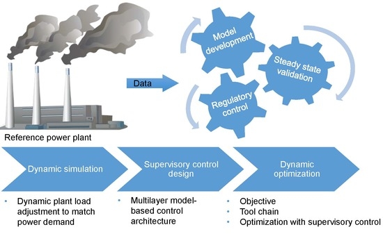
1. Introduction
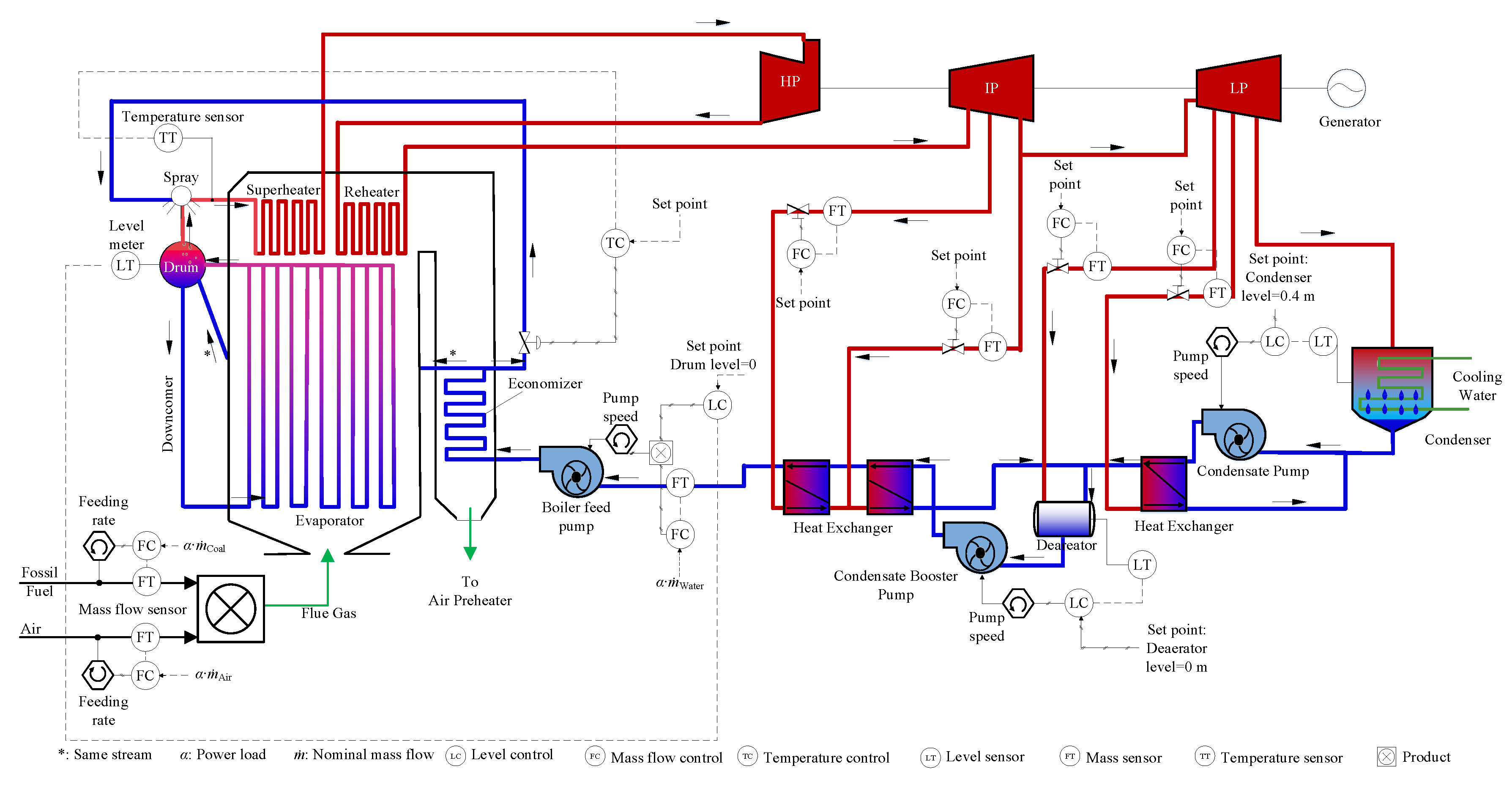
2. Power Plant Studied and Plant Model
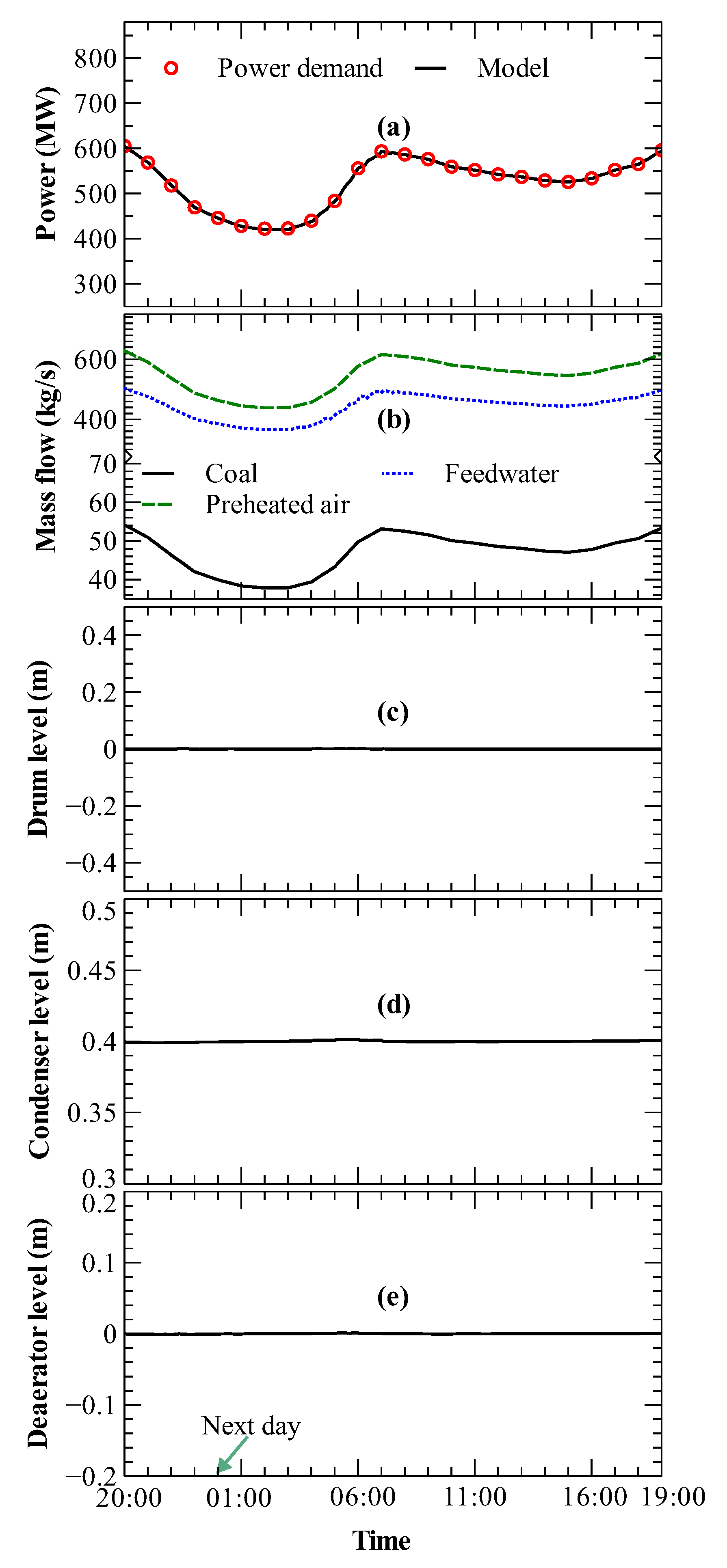
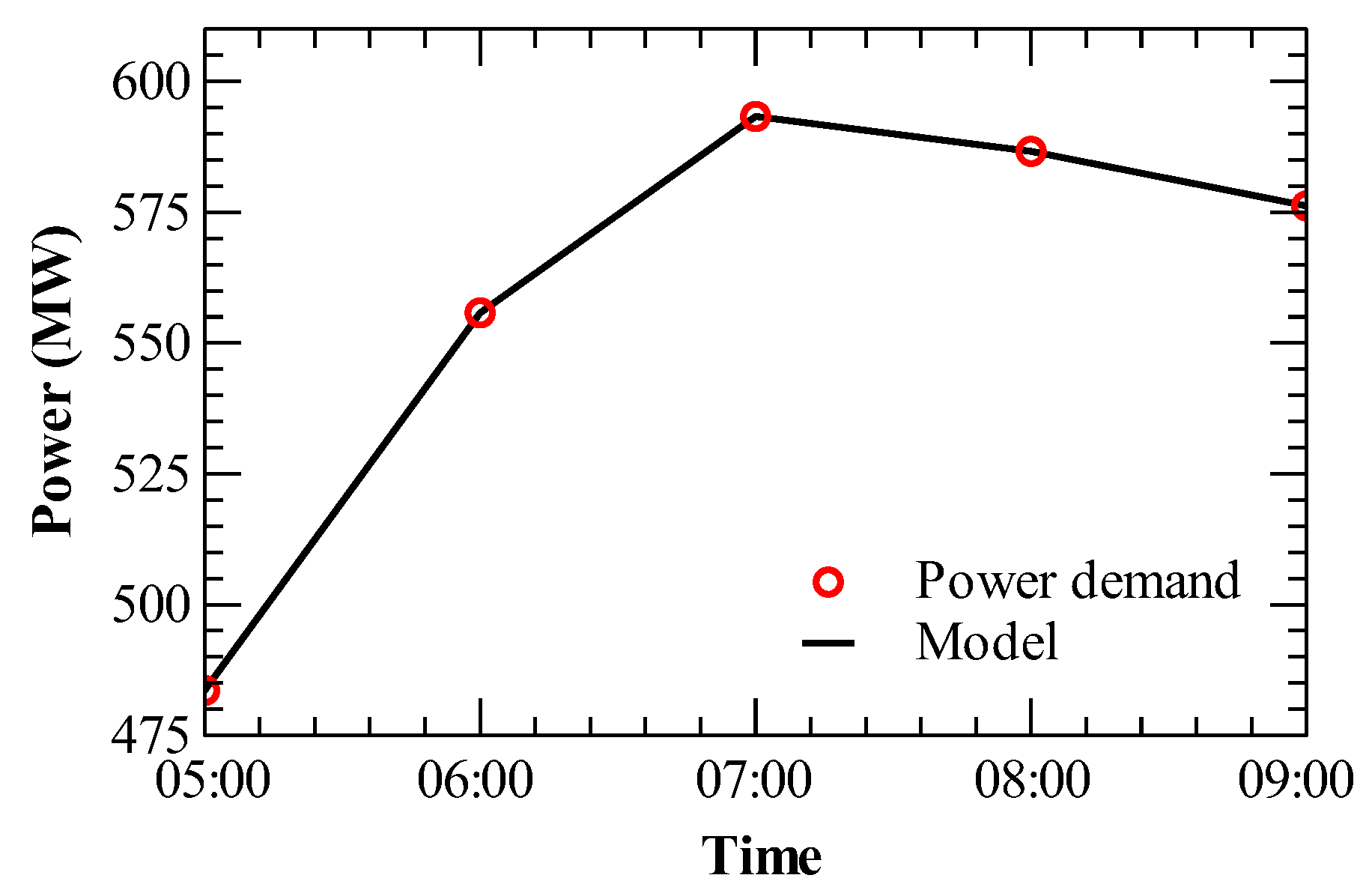
3. Power Plant Under Time-Varying Power Demand
4. Optimization of an Integrated Power Plant
4.1. Objective and Optimization Variables
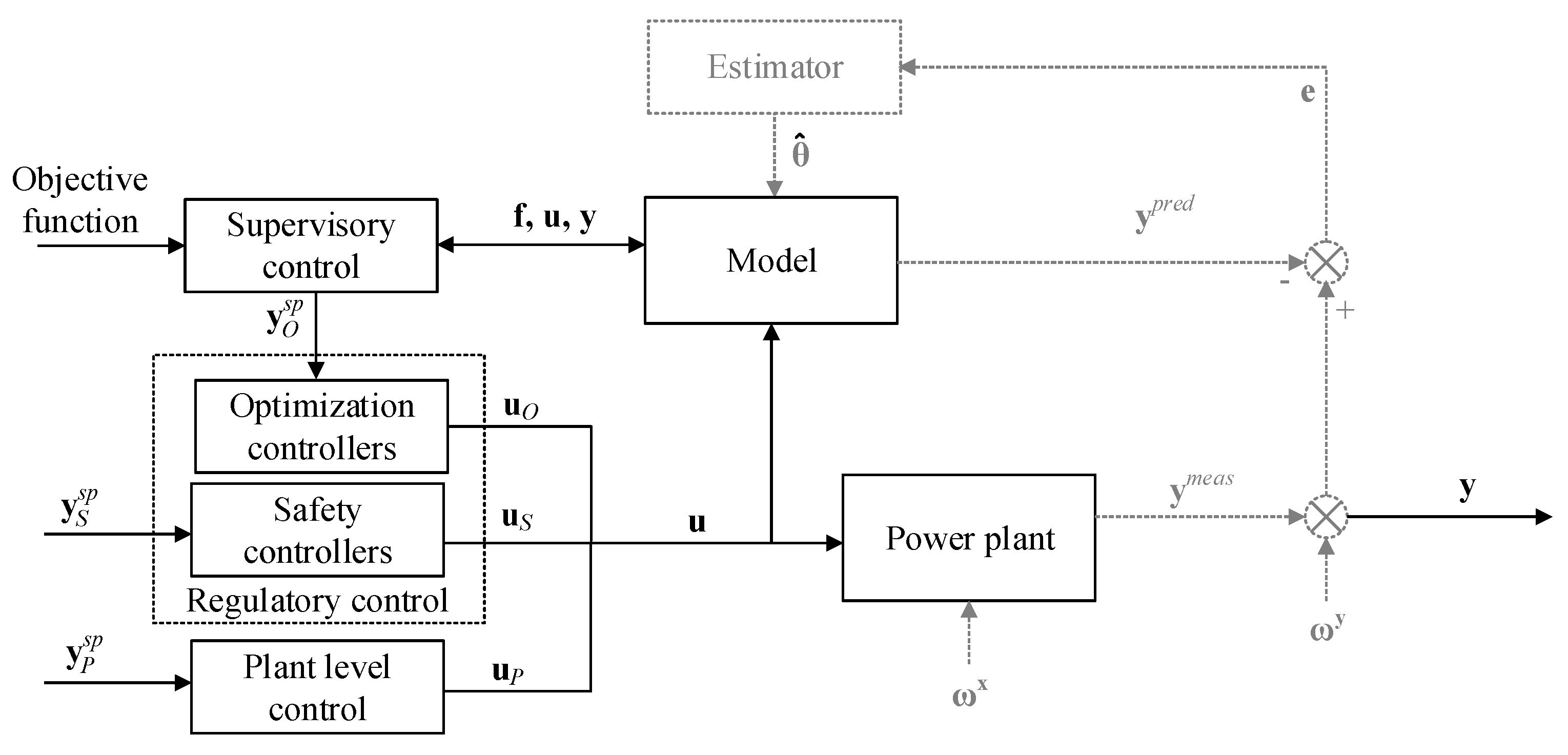
4.2. Supervisory Control
4.3. Optimization Formulation
5. Results
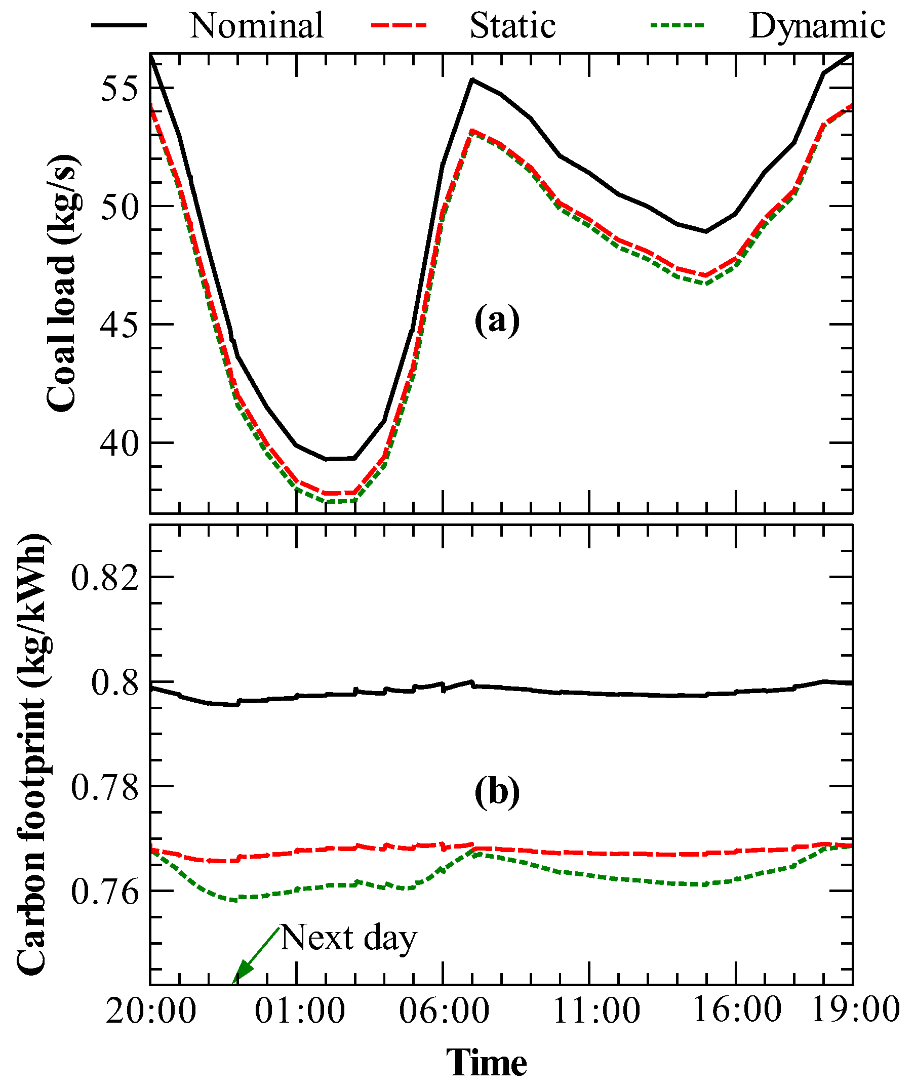
5.1. Case Study I: Optimization Variables and
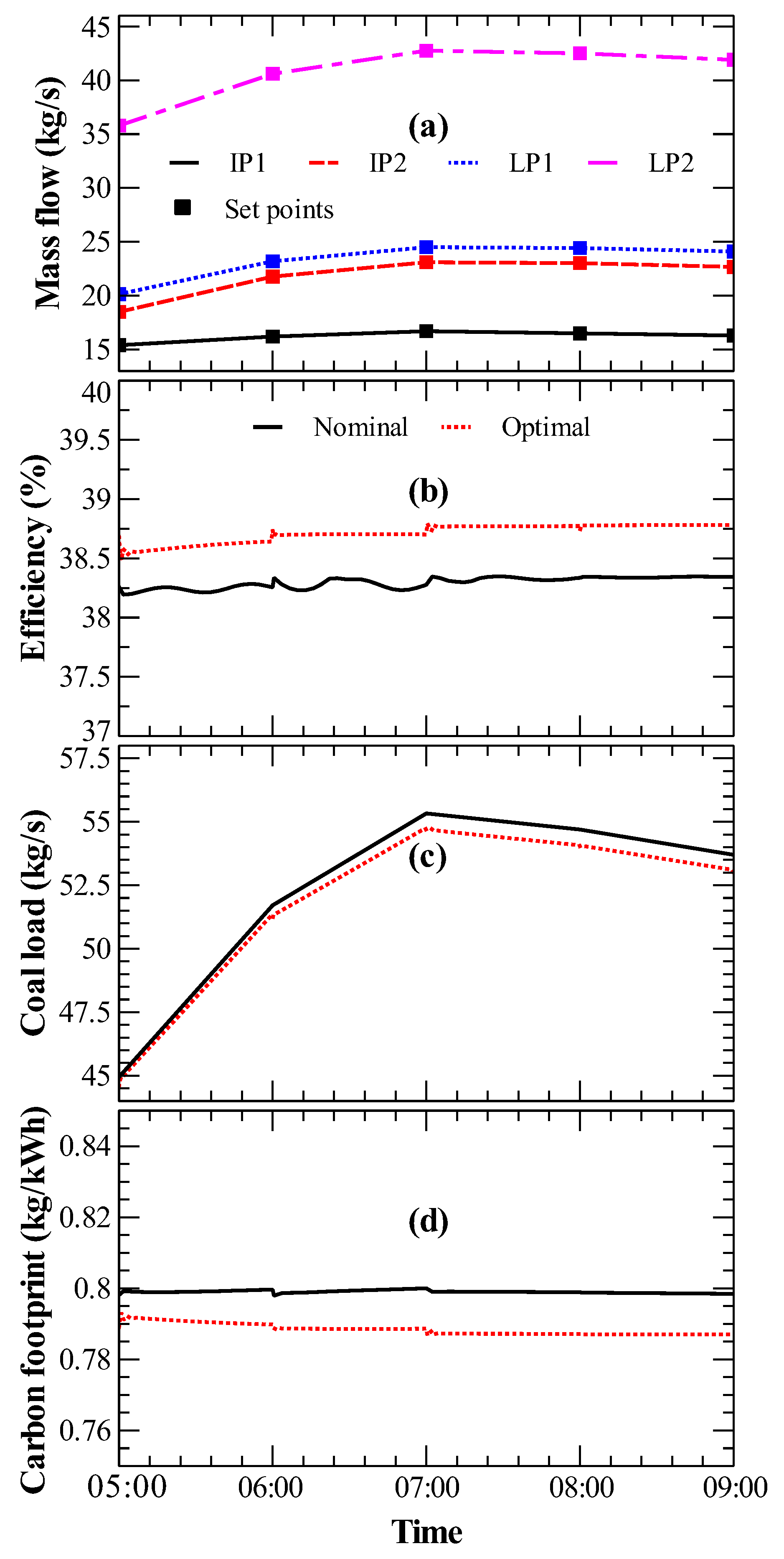
5.2. Case Study II: Optimization Variables , , and
6. Conclusions
Author Contributions
Funding
Acknowledgments
Conflicts of Interest
References
- Han, L.; Bollas, G.M. Chemical-looping combustion in a reverse-flow fixed bed reactor. Energy 2016, 102, 669–681. [Google Scholar] [CrossRef]
- Han, L.; Bollas, G.M. Dynamic optimization of fixed bed chemical-looping combustion processes. Energy 2016, 112, 1107–1119. [Google Scholar] [CrossRef]
- Ibrahim, T.K.; Mohammed, M.K.; Awad, O.I.; Rahman, M.; Najafi, G.; Basrawi, F.; Abd Alla, A.N.; Mamat, R. The optimum performance of the combined cycle power plant: A comprehensive review. Renew. Sustain. Energy Rev. 2017, 79, 459–474. [Google Scholar] [CrossRef]
- Viswanathan, R.; Henry, J.; Tanzosh, J.; Stanko, G.; Shingledecker, J.; Vitalis, B.; Purgert, R. U.S. Program on Materials Technology for Ultra-Supercritical Coal Power Plants. J. Mater. Eng. Perform. 2005, 14, 281–292. [Google Scholar] [CrossRef]
- Hasler, D.; Rosenquist, W.; Gaikwad, R. New coal-fired power plant performance and cost estimates. In Sargent and Lundy Project; Environmental Protection Agency: Washington, DC, USA, 2009; pp. 1–82. [Google Scholar]
- Cziesla, F. Lünen—State-of-theArt Ultra Supercritical Steam Power Plant Under Construction Andreas Senzel. In Proceedings of the Power Generation Europe 2009, Cologne, Germany, 26–29 May 2009; pp. 1–21. [Google Scholar]
- U.S. Energy Information Administration. Energy Information Administration: Annual Energy Outlook 2018; U.S. Energy Information Administration: Washington, DC, USA, 2018.
- Masters, G.M. Renewable and Efficient Electric Power Systems; John Wiley & Sons, Inc.: Hoboken, NJ, USA, 2004; p. 712. [Google Scholar] [CrossRef]
- Shah, R.; Mithulananthan, N.; Bansal, R. Oscillatory stability analysis with high penetrations of large-scale photovoltaic generation. Energy Convers. Manag. 2013, 65, 420–429. [Google Scholar] [CrossRef]
- Edmunds, R.; Davies, L.; Deane, P.; Pourkashanian, M. Thermal power plant operating regimes in future British power systems with increasing variable renewable penetration. Energy Convers. Manag. 2015, 105, 977–985. [Google Scholar] [CrossRef]
- Critz, D.K.; Busche, S.; Connors, S. Power systems balancing with high penetration renewables: The potential of demand response in Hawaii. Energy Convers. Manag. 2013, 76, 609–619. [Google Scholar] [CrossRef]
- Eser, P.; Singh, A.; Chokani, N.; Abhari, R.S. Effect of increased renewables generation on operation of thermal power plants. Appl. Energy 2016, 164, 723–732. [Google Scholar] [CrossRef]
- Fu, C.; Anantharaman, R.; Jordal, K.; Gundersen, T. Thermal efficiency of coal-fired power plants: From theoretical to practical assessments. Energy Convers. Manag. 2015, 105, 530–544. [Google Scholar] [CrossRef]
- Sanpasertparnich, T.; Aroonwilas, A. Simulation and optimization of coal-fired power plants. Energy Procedia 2009, 1, 3851–3858. [Google Scholar] [CrossRef]
- Tzolakis, G.; Papanikolaou, P.; Kolokotronis, D.; Samaras, N.; Tourlidakis, A.; Tomboulides, A. Simulation of a coal-fired power plant using mathematical programming algorithms in order to optimize its efficiency. Appl. Therm. Eng. 2012, 48, 256–267. [Google Scholar] [CrossRef]
- Elmqvist, H.; Brück, D.; Otter, M. Dymola User’s Manual; Dynasim AB: Lund, Sweden, 1996. [Google Scholar]
- Process Systems Enterprise. gPROMS Advanced User Guide; Process Systems Enterprise Limited: London, UK, 2004. [Google Scholar]
- Chen, C.; Han, L.; Bollas, G.M. Dynamic Simulation of Fixed-Bed Chemical-Looping Combustion Reactors Integrated in Combined Cycle Power Plants. Energy Technol. 2016, 4, 1209–1220. [Google Scholar] [CrossRef]
- Franke, R.; Babji, B.; Antoine, M.; Isaksson, A. Model-based online applications in the ABB Dynamic Optimization framework. In Proceedings of the 6th International Modelica Conference, Bielefeld, Germany, 3–4 March 2008; pp. 279–285. [Google Scholar]
- Modelica Association. Modelica—A Unified Object-Oriented Language for Physical Systems Modeling. In Proceedings of the 12th European Conference on Object-Oriented Programming, Brussels, Belgium, 20–24 July 2010. [Google Scholar]
- Lind, A.; Sällberga, E.; Velutb, S. Start-up Optimization of a Combined Cycle Power Plant. In Proceedings of the 9th International Modelica Conference, Munich, Germany, 3–5 September 2012. [Google Scholar]
- Skogestad, S. Control structure design for complete chemical plants. Comput. Chem. Eng. 2004, 28, 219–234. [Google Scholar] [CrossRef]
- Lestage, R.; Pomerleau, A.; Hodouin, D. Constrained real-time optimization of a grinding circuit using steady-state linear programming supervisory control. Powder Technol. 2002, 124, 254–263. [Google Scholar] [CrossRef]
- Baillie, B.P.; Bollas, G.M. Development, Validation, and Assessment of a High Fidelity Chilled Water Plant Model. Appl. Therm. Eng. 2017, 111, 477–488. [Google Scholar] [CrossRef]
- Mittal, K.; Wilson, J.; Baillie, B.; Gupta, S.; Bollas, G.; Luh, P.B. Supervisory Control for Resilient Chiller Plants under Condenser Fouling. IEEE Access 2017, 5, 14028–14046. [Google Scholar] [CrossRef]
- Sáez, D.; Ordys, A.; Grimble, M. Design of a supervisory predictive controller and its application to thermal power plants. Optim. Control Appl. Methods 2005, 26, 169–198. [Google Scholar] [CrossRef]
- Ponce, C.V.; Sáez, D.; Bordons, C.; Núñez, A. Dynamic simulator and model predictive control of an integrated solar combined cycle plant. Energy 2016, 109, 974–986. [Google Scholar] [CrossRef]
- Chen, C.; Zhou, Z.; Bollas, G.M. Dynamic modeling, simulation and optimization of a subcritical steam power plant. Part I: Plant model and regulatory control. Energy Convers. Manag. 2017, 145, 324–334. [Google Scholar] [CrossRef]
- Joseph, G.; Singer, P. (Eds.) Combustion Fossil Power: A Reference Book on Fuel Burning and Steam Generation, 4th ed.; Combustion Engineering: New York, NY, USA, 1991. [Google Scholar]
- ISO New England. Real-Time Maps and Charts; ISO New England: Holyoke, MA, USA, 2016. [Google Scholar]
- Casella, F.; Leva, A. Modelica open library for power plant simulation: Design and experimental validation. In Proceedings of the 2003 Modelica Conference, Linkoping, Sweden, 3–4 November 2003. [Google Scholar]
- Hsu, C.; Chen, C. Applications of improved grey prediction model for power demand forecasting. Energy Convers. Manag. 2003, 44, 2241–2249. [Google Scholar] [CrossRef]
- Akay, D.; Atak, M. Grey prediction with rolling mechanism for electricity demand forecasting of Turkey. Energy 2007, 32, 1670–1675. [Google Scholar] [CrossRef]
- Starkloff, R.; Alobaid, F.; Karner, K.; Epple, B.; Schmitz, M.; Boehm, F. Development and validation of a dynamic simulation model for a large coal-fired power plant. Appl. Therm. Eng. 2015, 91, 496–506. [Google Scholar] [CrossRef]
- ABB and Rocky Mountain Institute. ABB Energy Efficiency Handbook: Power Generation—Energy Efficient Design of Auxiliary Systems in Fossil-Fuel Power Plants; Technical Report; ABB and Rocky Mountain Institute: Basalt, CO, USA, 2009. [Google Scholar]
- Sanpasertparnich, T.; Aroonwilas, A.; Veawab, A. Improved Thermal Efficiency of Coal-Fired Power Station: Monte Carlo Simulation. In Proceedings of the 2006 IEEE EIC Climate Change Conference, Ottawa, ON, Canada, 10–12 May 2006; pp. 1–9. [Google Scholar] [CrossRef]
- Lizon-A-Lugrin, L.; Teyssedou, A.; Pioro, I. Appropriate thermodynamic cycles to be used in future pressure-channel supercritical water-cooled nuclear power plants. Nucl. Eng. Des. 2012, 246, 2–11. [Google Scholar] [CrossRef]
- Suresh, M.V.J.J.; Reddy, K.S.; Kolar, A.K. Thermodynamic Optimization of Advanced Steam Power Plants Retrofitted for Oxy-Coal Combustion. J. Eng. Gas Turbines Power 2011, 133, 063001. [Google Scholar] [CrossRef]
- Suresh, M.; Reddy, K.; Kolar, A.K. ANN-GA based optimization of a high ash coal-fired supercritical power plant. Appl. Energy 2011, 88, 4867–4873. [Google Scholar] [CrossRef]
- Wang, L.; Yang, Y.; Dong, C.; Morosuk, T.; Tsatsaronis, G. Multi-objective optimization of coal-fired power plants using differential evolution. Appl. Energy 2014, 115, 254–264. [Google Scholar] [CrossRef]
- Xiong, J.; Zhao, H.; Zhang, C.; Zheng, C.; Luh, P.B. Thermoeconomic operation optimization of a coal-fired power plant. Energy 2012, 42, 486–496. [Google Scholar] [CrossRef]
- Koch, C.; Cziesla, F.; Tsatsaronis, G. Optimization of combined cycle power plants using evolutionary algorithms. Chem. Eng. Process 2007, 46, 1151–1159. [Google Scholar] [CrossRef]
- Espatolero, S.; Cortés, C.; Romeo, L.M. Optimization of boiler cold-end and integration with the steam cycle in supercritical units. Appl. Energy 2010, 87, 1651–1660. [Google Scholar] [CrossRef]
- Regulagadda, P.; Dincer, I.; Naterer, G.F. Exergy analysis of a thermal power plant with measured boiler and turbine losses. Appl. Therm. Eng. 2010, 30, 970–976. [Google Scholar] [CrossRef]
- Kakaras, E.; Ahladas, P.; Syrmopoulos, S. Computer simulation studies for the integration of an external dryer into a Greek lignite-fired power plant. Fuel 2002, 81, 583–593. [Google Scholar] [CrossRef]
- Tatjewski, P. Advanced Control of Industrial Processes; Advances in Industrial Control Series; Springer: London, UK, 2007. [Google Scholar] [CrossRef]
- The MathWorks Inc. MATLAB; MathWorks: Natick, MA, USA, 2013. [Google Scholar]
- MODELISAR Consortium. Functional Mock-up Interface for Model Exchange; Version 1.0; MODELISAR Consortium: Linköping, Sweden, 2010. [Google Scholar]
- Chaibakhsh, A.; Ghaffari, A. Steam turbine model. Simul. Model. Pract. Theory 2008, 16, 1145–1162. [Google Scholar] [CrossRef]


| Feed-Forward Control: Air and Feedwater Controllers | ||||
| Controlled variables | ||||
| PID (Proportional-Integral-Derivative) Control: Fuel Load Controller | ||||
| Controlled variables | Manipulated variables | |||
| P | ||||
| Ref. | (%) | Optimization Variables | ||||||
|---|---|---|---|---|---|---|---|---|
| (C) | /// (kg/s) | (C) | (kg/s) | (bar) | (%) | Others | ||
| [14,36] | 7.8 | [530,600] | [3.9,19.6]/ [6.2,43.3]/ [15.1,28.7]/ [11.1,42.1] | [166,190] | [250,350] | [166,190] | [11.1,17.6] | |
| [15] | 0.55 | [0,30.8]/ [0,51.2]/ [0,21.1]/ [0,0.94] | ||||||
| [37] | 0.41 | [600,625] | [16,26]/ [14,24]/ [12.6,24]/ [34,57] | [400,475] | [20,30] | |||
| [38,39] | 2.8 | [550,700] | [35,275] | [230,350] | Excess air ∈ [0,25%], [580,620] | |||
| [40] | 2 | [550,700] | [230,350] | [0.75,0.87], (bar) ∈ [60/9/0.0356, 80/25.5/2.68] | ||||
| [13] | 5.9 | [487,1076] | [150,450] | |||||
| [41] | 2.5 | [535,545] | ∈ [0.8,0.95] | |||||
| [42] | 1.3 | [485,537] | [45,57] | |||||
| [43] | 0.79 | [115,278] | [21,38.4] | ( C) ∈ [85,125] | ||||
| [44] | 3.5 | [460,530] | [64,110] | (bar) ∈ [0.01,0.05] | ||||
| Case I | ||||
| Admissible Inputs () | (C) | (C) | ||
| Min | 520 | 150 | ||
| Max | 610 | 250 | ||
| Case II | ||||
| Admissible Inputs a () | (kg/s) | (kg/s) | (kg/s) | (kg/s) |
| Min | 16 | 10 | 10 | 28 |
| Max | 28 | 28 | 28 | 47 |
| Temporal Inputs b | ||||
| 1 | ||||
| 24 for case I (4 for case II) | ||||
| System Output | Nominal | Optimal |
|---|---|---|
| (C) | 538 | 560 |
| (C) | 200 | 248 |
| (%) | 38.3 | 40.23 |
| (kg/s) | 56.38 | 54.25 |
| carbon footprint (kg/kWh) | 0.8 | 0.77 |
| Output | Static Optimization | Dynamic Optimization |
|---|---|---|
| (tons/day) | 160.9 | 184.8 |
| (kg/kWh) | 0.0303 | 0.0351 |
| (tons/day) | 440.2 | 511.9 |
| Controllers | IP1 | IP2 | LP1 | LP2 |
|---|---|---|---|---|
| Controlled variables | ||||
| Manipulated variables | Valve opening | Valve opening | Valve opening | Valve opening |
| 0.1 | 0.1 | 0.1 | 0.1 | |
| 0.0001 | 0.0001 | 0.0001 | 0.0001 |
| System Output | Nominal | Optimal |
|---|---|---|
| (kg/s) | 27.4 | 16.8 |
| (kg/s) | 14 | 23.1 |
| (kg/s) | 16.5 | 23.7 |
| (kg/s) | 30 | 43.8 |
| (%) | 38.3 | 38.78 |
| (kg/s) | 56.38 | 55.68 |
| Carbon footprint (kg/kWh) | 0.8 | 0.79 |
© 2018 by the authors. Licensee MDPI, Basel, Switzerland. This article is an open access article distributed under the terms and conditions of the Creative Commons Attribution (CC BY) license (http://creativecommons.org/licenses/by/4.0/).
Share and Cite
Chen, C.; Bollas, G.M. Dynamic Optimization of a Subcritical Steam Power Plant Under Time-Varying Power Load. Processes 2018, 6, 114. https://doi.org/10.3390/pr6080114
Chen C, Bollas GM. Dynamic Optimization of a Subcritical Steam Power Plant Under Time-Varying Power Load. Processes. 2018; 6(8):114. https://doi.org/10.3390/pr6080114
Chicago/Turabian StyleChen, Chen, and George M. Bollas. 2018. "Dynamic Optimization of a Subcritical Steam Power Plant Under Time-Varying Power Load" Processes 6, no. 8: 114. https://doi.org/10.3390/pr6080114
APA StyleChen, C., & Bollas, G. M. (2018). Dynamic Optimization of a Subcritical Steam Power Plant Under Time-Varying Power Load. Processes, 6(8), 114. https://doi.org/10.3390/pr6080114