Challenges in Nanofluidics—Beyond Navier–Stokes at the Molecular Scale


1
School of Science and Centre for Molecular and Nanoscale Physics, RMIT University, GPO Box 2476, Melbourne, Victoria 3001, Australia
2
Department of Mathematics, School of Science, Faculty of Science, Engineering and Technology, Swinburne University of Technology, PO Box 218, Hawthorn, Victoria 3122, Australia
*
Authors to whom correspondence should be addressed.
†
Both authors contributed to this work, with P.J.D. taking the leading role in writing the manuscript.
Processes 2018, 6(9), 144; https://doi.org/10.3390/pr6090144
Submission received: 18 July 2018
/
Revised: 17 August 2018
/
Accepted: 21 August 2018
/
Published: 1 September 2018
(This article belongs to the Special Issue Transport of Fluids in Nanoporous Materials)
Abstract
:The fluid dynamics of macroscopic and microscopic systems is well developed and has been extensively validated. Its extraordinary success makes it tempting to apply Navier–Stokes fluid dynamics without modification to systems of ever decreasing dimensions as studies of nanofluidics become more prevalent. However, this can result in serious error. In this paper, we discuss several ways in which nanoconfined fluid flow differs from macroscopic flow. We give particular attention to several topics that have recently received attention in the literature: slip, spin angular momentum coupling, nonlocal stress response and density inhomogeneity. In principle, all of these effects can now be accurately modelled using validated theories. Although the basic principles are now fairly well understood, much work remains to be done in their application.

1. Introduction
The classical Navier–Stokes theory describing flow of Newtonian fluids has been remarkably successful, but it is inadequate under certain conditions. If the rate of deformation is high, nonlinear effects such as a shear rate dependent viscosity and normal stress differences may become apparent. If the frequency of oscillatory deformation is high, we may observe viscoelastic effects related to the elastic storage and release of energy. These effects are now quite well understood and can be described using standard treatments of non-Newtonian fluid mechanics [1]. Generally speaking, the theory of fluid flow at macroscopic and microscopic scales is successful and well developed. However, when Navier–Stokes fluid dynamics and its extensions to shear rate dependent and frequency dependent constitutive relations are applied to nano-confined flows, the theory can fail. New physical effects become important and serious errors and inconsistencies can arise if the methods of macroscopic fluid mechanics are used without modification.
The reason for this is that several effects that are negligible or absent in macroscopic flows may become significant or even dominant in nanoflows. Wall slip, spin angular momentum coupling, spatially nonlocal response, and nonlinear, nonlocal coupling of the shear pressure and velocity gradient to a strongly inhomogeneous density field can all modify the flow of a fluid under strong confinement. Recent studies have shown that all of these effects can be successfully modelled. Experimental studies of fluid flow are steadily being extended to smaller and smaller system sizes, but computer simulations have a unique advantage in studies of nanoconfined fluid flow. They are ideally suited to studies of nanoflows because the system sizes and timescales that are accessible in computer simulations match the relevant size and timescales. In addition, computer simulations allow us to study velocity, density and shear pressure profiles at resolutions that would be impossible to achieve experimentally.
In this paper, we review some recent advances in the fluid dynamics of nanoconfined liquids, placing them in context and discussing the conditions under which they become important. In this work, we focus on single component fluids. To study multicomponent systems, we would need to include the composition as an additional variable and consider the many ways that the composition couples to the effects that are already present for pure fluids. Likewise, we have not considered electrical effects, which are so important in microfluidic and lab on a chip systems. These topics have been discussed in detail by other authors [2,3,4,5], and we urge interested readers to consult their work. We assume that all flows discussed are time independent, so we restrict our attention to steady states, but it is worth mentioning that nanoscale viscoelasticity remains largely unexplored.
2. Slip
In most macroscopic flow situations, a stick boundary condition, where the fluid velocity at the wall is taken to be equal to the wall velocity, is assumed. At the macroscopic scale, it is only in extreme cases that we must allow for slip, for example when we have plug flow of a paste or polymer melt, or when trapped gas bubbles in superhydrophobic surfaces lead to extreme slip [6]. However, even simple liquids can experience some slip. Strong slip is expected for water flowing near hydrophobic surfaces such as graphene or carbon nanotubes. Given a suitable surface structure, slip can also be observed for relatively hydrophilic surfaces [7]. For Poiseuille flow through a wide channel, the slip velocity, defined as the difference between the wall velocity and the fluid velocity at the wall, is only a very small fraction of the maximum velocity of the fluid in the channel, and so it is safely approximated as zero. On the other hand, for very narrow channels of nanometre scale, the slip velocity can be a significant fraction of the maximum velocity in the channel. Predictions of flow rates based on the assumption of the no-slip boundary condition can therefore be significantly in error, underestimating the true flow rate.
Here, we focus on the slip that occurs at the atomic scale on atomically smooth surfaces, sometimes known as intrinsic slip. Slip that occurs on a larger length scale, involving structured or patterned surfaces, roughness and chemical heterogeneity has been discussed by other authors [8].
The slip velocity depends on the strain rate at the wall and is not a material property. The relevant material property describing slip is the slip friction coefficient, defined below. The ratio of the fluid viscosity to the slip friction coefficient gives us another material property (really a property of the interface between the two materials), called the slip length. Very high spatial resolution measurements of the flow velocity of aqueous solutions near a hydrophobic wall, for example, have shown slip lengths of 80–100 nm [9]. The slip length of water confined by highly hydrophobic graphene and carbon nanotube surfaces has been computed to be around 60 nm, but there is enormous variation in both experimental and simulation results [10], due partly to subtle differences in simulation technique [11] and molecular models, but also error prone data analysis [12] and experimental difficulties. The consensus of careful simulation and experimental studies of flow of water on molecularly smooth hydrophobic surfaces is that slip lengths on these surfaces typically vary from nanometres up to tens of nanometres [10]. Because it has been difficult to reproduce the much larger experimental values sometimes found, it is possible that measurements of some of the larger values could suffer from uncontrolled experimental factors, such as dissolved or trapped gases [13], surface roughness and imperfections [14] or other yet unidentified factors.
One of the difficulties with computation of the slip length and slip friction coefficient by direct evaluation in non-equilibrium molecular dynamics that simulate flow through a channel is thatk for high slip systems, the velocity profile is almost flat. Extrapolation of such a velocity profile to the position where the velocity is zero is extremely error prone [12]. Methods based on equilibrium correlation functions do not suffer from these problems. Several theoretical discussions of correlation function methods for computation of the slip friction coefficient have been published [15,16,17,18,19,20] but there is still some doubt concerning the agreement between the different forms. Here, we describe a simple one [18] that has been extensively validated by comparison with both nonequilibrium simulations and experimental results [10,12,21,22,23].
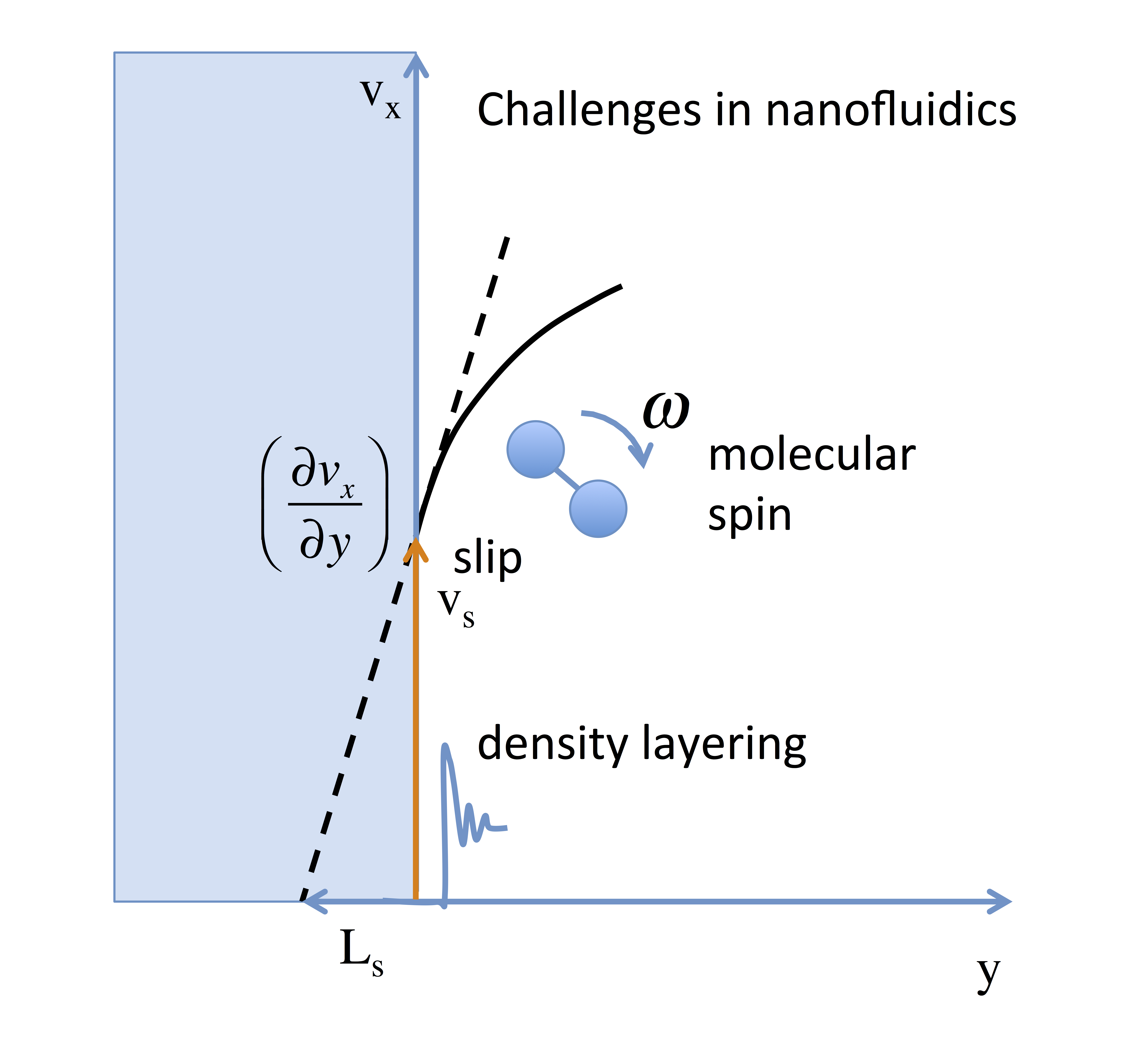
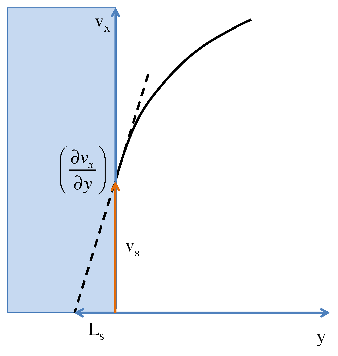
Navier’s slip friction coefficient is defined as the proportionality coefficient relating the shear pressure at the wall to the velocity difference between the wall and the fluid , which we call the slip velocity
where we assume that the flow is in the x direction and the velocity gradient is in the y direction. The flow geometry for flow in the x direction adjacent to a flat solid wall is shown in Figure 1.
The viscous pressure in the fluid at the wall is given by Newton’s law of viscosity
where is the shear viscosity at zero shear rate. Since the shear pressure must be continuous, both values of the shear pressure must be equal. Eliminating the shear pressure, we find
which defines the slip length as
To derive a correlation function expression for the slip friction coefficient, we must introduce a generalised constitutive equation that describes the fluctuations [18]. It is convenient to formulate this in terms of the wall–fluid shear force, given by
where A is the area over which the slip frictional force acts, is the friction kernel and is the random component of the shear pressure. Now, we multiply both sides of the constitutive equation by the slip velocity and ensemble average to form the correlation functions
where
When this equation is Laplace transformed, we find
The friction kernel is well approximated by a sum of exponentials [18],
which has the Laplace transform
In practice, a single exponential is often sufficient [18,21]. The amplitudes and decay rates of the exponentials can then be obtained from fits to the Laplace transformed correlation functions.
From the computational point of view, the wall–fluid shear force is easily evaluated in computer simulations. The slip velocity is more problematic. One way to evaluate it would be to fit the instantaneous velocity profile each time the correlation functions are evaluated. However, this requires the assumption of a fitting function, which could be biassed. Another way is to evaluate the instantaneous velocity of the fluid averaged over a region within a distance of the wall. This has the disadvantage that averaging over a finite region could also result in error, but the calculation of the slip friction coefficient for a given wall–fluid combination can be repeated for different values of , and the most physically meaningful value of the slip friction coefficient chosen. In practice, it is straightforward to choose the most physically meaningful value of the slip friction coefficient because it quickly increases to a broad maximum (plateau) value as is increased, before steadily decreasing thereafter. This maximum value usually occurs when is approximately equal to one molecular diameter. Choosing this value of the slip friction coefficient gives excellent agreement with the results of nonequilibrium molecular dynamics simulations [18,21].
This method has been used to evaluate the slip friction coefficient and the slip length of a simple Lennard–Jones type atomic fluid near a solid planar LJ wall [18] and a graphene wall [21] and more complex molecular fluids such as water against both Lennard–Jones atomic walls and graphene [12]. It has also been adapted to a cylindrical geometry [22] for studies of the slip friction coefficient of water in carbon nanotubes [10,23].
3. Spin Angular Momentum Coupling
It is well known that extended molecules spin in a shear field [24]. What is less well known is that the spin angular velocity is coupled to the translational velocity. This coupling is usually negligible in macroscopic flows, but it can become significant at the nanoscale.
To describe this effect, we begin with the extended Navier–Stokes equations for stable flow in a planar flow geometry (where the convective terms are zero), which are obtained by inserting the relevant linear transport equations into the balance equations for the translational and angular momentum [25,26],
The first of these describes the evolution of the translational fluid streaming velocity in the flow direction . A new transport coefficient, the rotational viscosity , which governs the relaxation of spin angular momentum appears in addition to the usual shear viscosity, . The rotational (or vortex) viscosity describes the rate of conversion between fluid vorticity and molecular spin angular momentum . If , then we just have the usual Navier–Stokes equation. In the absence of a pressure gradient (omitted from this equation since it is zero for field driven flows in our flow geometry), flow can be generated by the external body force density , but if this is also zero, we see that it is also possible to have a flow driven by the gradient of the angular velocity. We will return to this point later. The second equation, which describes the evolution of the molecular spin angular velocity field includes a diffusive term involving the sum of the spin viscosities as well as the rotational viscosity . The spin viscosity describes the diffusive flux of spin angular momentum due to the traceless symmetric part of the spin angular velocity gradient, while describes the diffusive flux of spin angular momentum due to the antisymmetric part of the spin angular velocity gradient [25]. These transport coefficients have been evaluated for some molecular fluids, including water [27]. Again, there is a term that accounts for external fields, this time in the form of an external body torque density .
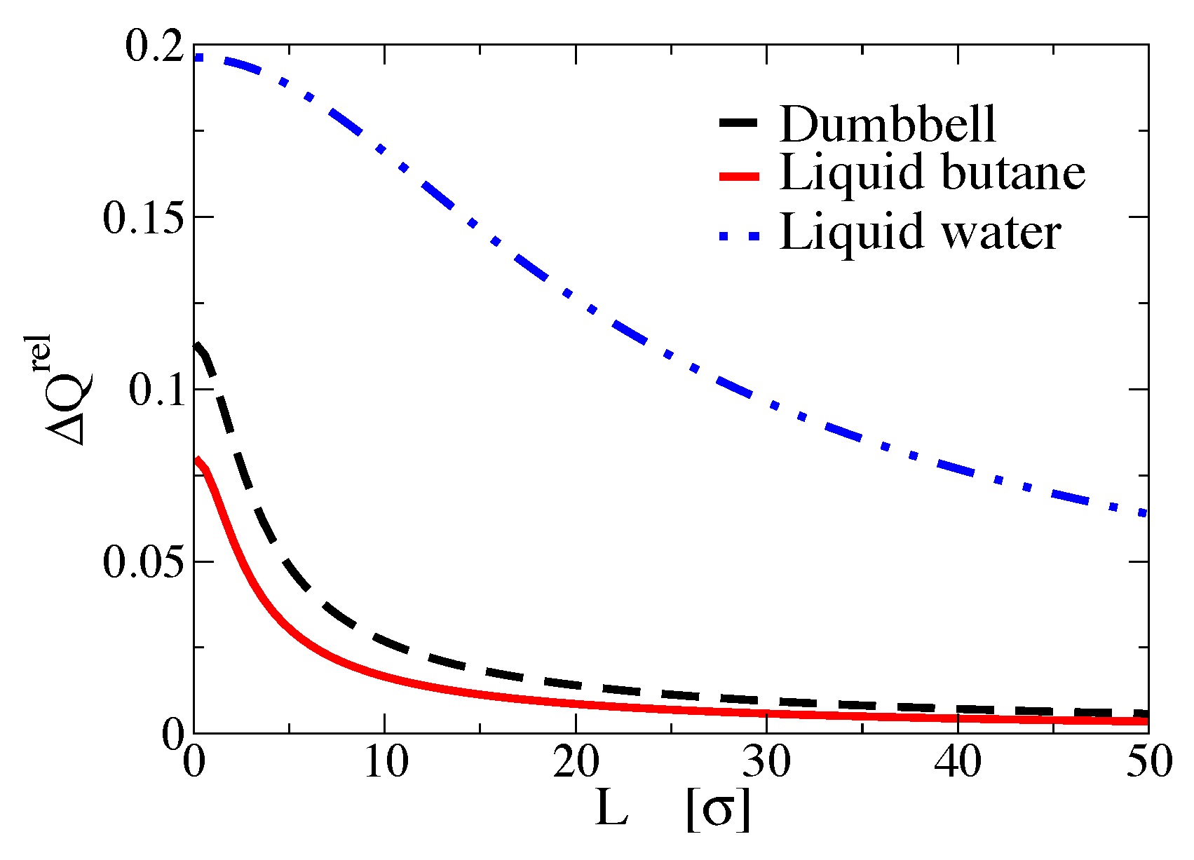
When applied to planar Poiseuille flow through a narrow channel driven by an external body force density , these equations predict a difference between the velocity field calculated from the Navier–Stokes equation alone compared to the results of the extended Navier–Stokes equations including the spin coupling. Simulations of a molecular fluid consisting of extended linear molecules (buta-triene) show that the flow rate difference is small for channels of width greater than 7 nm, but it grows to around 10% at a channel width of 1 nm [28]. For very narrow channels, accurate prediction of flow rates and velocity profiles requires consideration of the extended Navier–Stokes equations [26,28,29]. Figure 2 shows the flow rate reduction predicted by taking spin angular momentum coupling into account for nanoconfined flows of a dumbbell fluid, liquid butane and liquid water [26].
As mentioned above, a translational flow can be generated even in the absence of a translational body force if a body torque is applied instead. With symmetric boundary conditions (for example, with a stick boundary condition on both sides of the channel), equal flow is generated in both directions and no net flow results, but if the boundary conditions are asymmetric, with slip on one wall and stick on the other, a net flow results. This means that an external torque that spins the molecules can be used to pump a fluid. It has been demonstrated that a rotating electric field applied to polar molecules (such as water) under these conditions can generate a net flow in a nanochannel or nanotube, without the need for electrolyte or a pressure gradient [30,31].
4. Nonlocal Response
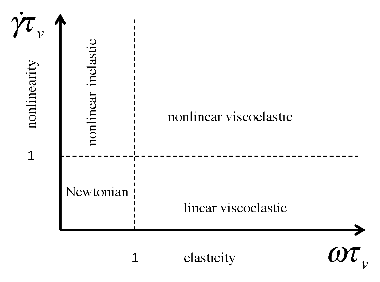
In macroscopic flows, the most common causes of non-Newtonian behaviour are nonlinear and viscoelastic deviations from Navier–Stokes behaviour. The Pipkin diagram [32] shown in Figure 3 schematically illustrates the different regions of fluid behaviour for typical macroscopic fluids. Here, we are interested in steady (zero frequency) flows so the Deborah number is zero.
In most macroscopic situations, spatial nonlocality is unimportant, except possibly when the system is near a glass transition [33] or the viscous correlation length is extraordinarily large for some other reason as it is for example in suspensions of long fibres that exhibit shear banding [34,35]. By contrast, in nanofluidic flows, spatial nonlocality can be a dominant effect that must be taken into account, even for ordinary molecular or atomic fluids. Deformations at sufficiently high wavenumber may differ strongly from homogeneous deformation, particularly in glassy liquids where dynamic heterogeneity with nanoscale dimensions is observed [33]. This means we must consider the concept of a spatially nonlocal response, where the stress at a point becomes a linear functional of the local deformation rate [36]. The stress at a point then depends not only on the strain rate at that point but also on the strain rate at nearby points. An alternative interpretation is that the stress depends not only on the velocity gradient but also on its derivatives, and so there is a contribution to the stress resulting from the spatial derivatives of the strain rate.
To describe spatially inhomogeneous steady state flows where the strain rate is independent of time but it varies strongly in space, we can introduce an analogue of the Pipkin diagram to characterise nonlocality, as shown in Figure 4. The viscous correlation length of the fluid, is measured by the width of the nonlocal viscosity kernel, defined in Equation (12). For situations where strong density inhomogeneity is also present (discussed below in this section), third and fourth axes could be added, representing the amplitude and spatial frequency of the density inhomogeneity. This diagram does not include these dimensions, so it represents nonlocal response for a uniform density fluid.
To account for the nonlocal response of the shear pressure to a steady velocity gradient of high spatial wavenumber, we apply a spatial convolution equation analogous to the linear viscoelastic constitutive equation
This is the most general linear relationship that we can postulate between the shear pressure and the velocity gradient or shear rate for a fluid with spatially homogeneous density where the strain rate varies only in the y-direction. The viscosity kernel weights the contribution of the strain rate at different distances from the point at which the shear pressure is evaluated. When , we expect the contribution of the shear rate to be greatest, and at larger values of , we expect the effect of the shear rate to be least, so should be a decreasing function of . At macroscopic length scales, it is reasonable to approximate as a constant multiplied by a Dirac delta function, and then the convolution integral simply reduces to Newton’s law of viscosity with a purely local response to the strain rate field.
A stringent test of this relationship can be made by applying a spatially sinusoidal transverse force to generate a sinusoidal velocity field. Since the velocity is sinusoidal, if the amplitude of the field is sufficiently small, the response is linear and the shear pressure response will also consist of a single sinusoidal component. When the wavelength of the sinusoidal driving force is sufficiently long (greater than a few molecular diameters) the shear pressure is just given by the Newtonian constitutive equation applied locally. In other words, the shear pressure at a given point depends only on the value of the strain rate at that point. However, when the wavelength of the strain rate oscillations is reduced to the order of a few molecular diameters, this procedure fails and the shear pressure is poorly reproduced. Using the nonlocal integral constitutive equation, it is possible to correctly predict the shear pressure, even when the velocity profile varies rapidly in space as displayed in Figure 5 [36].
In nanofluidic systems, it is possible for the strain rate to vary rapidly, and for a nonlocal response of the shear pressure to the rapidly varying strain rate to be observed. However, the rapid variation of the strain rate is also usually associated with rapid variation of the density of the fluid, due to strong molecular packing effects at the wall–fluid interface that occur even at equilibrium [37]. Therefore, we must consider the effect of spatial density variations on the velocity profile and the shear pressure profile.
5. Density Inhomogeneity
When a macroscopic fluid system has long wavelength density inhomogeneities, the assumption of constant transport coefficients in the Navier–Stokes equation is clearly inadequate. We can allow for this by making the linear transport coefficients position dependent through the position dependence of the density as well as, if necessary, the temperature and composition. In the simple case of density variation for an isothermal single component fluid, we would write Newton’s law of viscosity as
In a nanofluidic system, the fluid is almost always in contact with a solid wall. This induces strong oscillatory density variations near the wall, with local maxima that may exceed typical solid densities. Under these circumstances, it is obviously not viable to use the viscosity at the local density values. Bitsanis and coworkers [38,39] made a significant improvement on the local density model by proposing that the viscosity at a locally averaged value of the density could be used in the Newtonian viscosity equation. Despite the strong density variations near the wall, averaging over a sphere or planar layer of one to two molecular diameters gives an average density that is reasonably close to the liquid value, but still accounts for slow variations in the density. The constitutive equation for the local average density model in a planar geometry is then
with
This introduces an element of nonlocality into the constitutive equation for the shear pressure by making it dependent on the density averaged over a region surrounding the point of interest. The local averaged density model was successfully used by Bitsanis [38] to describe the velocity profile of a highly confined simple fluid. It has been extended by Hoang and Galliero [40,41,42], who investigated the effectiveness of different averaging kernels in the evaluation of the averaged density, and combined with a model for slip to provide a tractable and efficient hydrodynamic model for nanoflows by Bhadauria et al. [43,44]. The local average density model is, however, only a partial solution to the problem of describing the velocity profile for flow of a nanoconfined fluid. A major deficiency of this model is that it cannot account for the zeroes and velocity gradient reversals that can be seen in the velocity profiles of strongly confined fluids at high densities [45]. Strong molecular packing near the solid-fluid interface results in oscillations in the velocity profile that cannot possibly be described by the local average density model. Any constitutive equation that follows the same functional form as the simple Newtonian one would need to have infinite values of the viscosity at the points where the strain rate goes through zero, which is clearly unphysical. Therefore, we are again led to consider more general, nonlocal constitutive equations.
The fluid density inhomogeneity produced by wall–fluid interactions is uncontrolled. It is not possible to easily and independently control the amplitude and spatial frequency of the density oscillations due to the presence of a confining wall. To study nonlocal constitutive equations for the shear pressure, we need a more flexible framework. By applying a small amplitude sinusoidal longitudinal force (SLF) in a periodic simulation cell, it is possible to induce sinusoidal density variations [46] in a system with periodic boundaries and no explicit walls. When the amplitude of the applied force is increased, a nonlinear density response is generated. By adding together several sinusoidal forces of different frequency, it is possible to Fourier synthesise a spatially periodic density profile consistent with the periodic boundary conditions of the simulation cell that closely resembles the density profile seen in a nanoconfined fluid [47]. A sinusoidal transverse force (STF) can also be applied that generates flow. When both the longitudinal and transverse fields are applied together, we can generate flow in the presence of density inhomogeneity that can be controlled and manipulated at will [48,49].
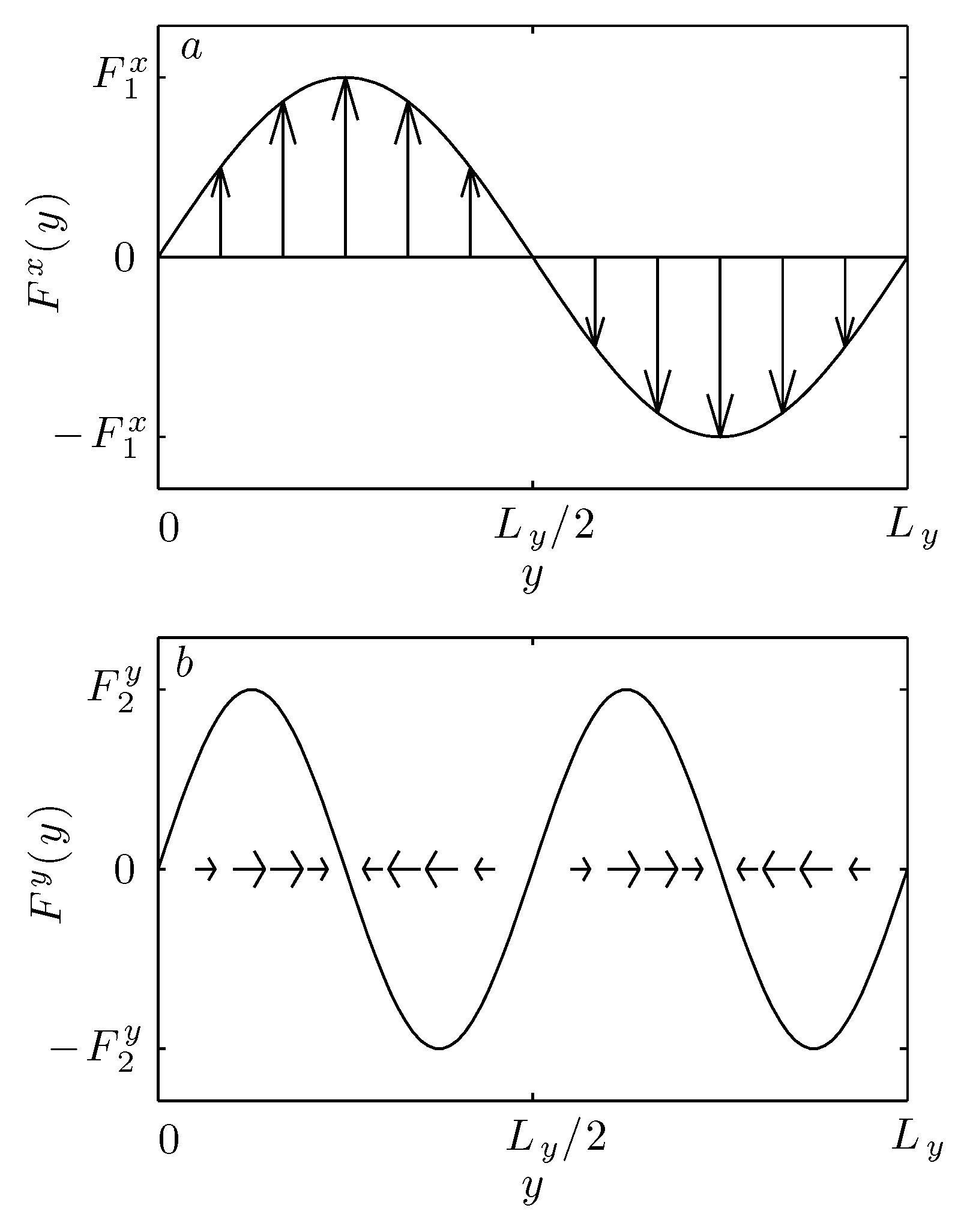
Considering a system where the external fields vary in the y direction, the combined longitudinal and transverse force can be represented as
Figure 6 schematically shows the two applied body forces.
The density response consists of contributions due to both the longitudinal and transverse forces. This is because the transverse force results in flow with a strain rate that varies in the y-direction. Heat is produced by the viscous dissipation associated with the velocity gradient, resulting in thermal expansion, which changes the density, in addition to the direct effect of the longitudinal force on the density. In general, the density response is given by a functional expansion that depends on both the longitudinal and transverse forces,
where and can be either x (transverse force) or y (longitudinal force) and the response functions are the functional derivatives
The response functions are evaluated at equilibrium. Due to the spatial symmetry of the equilibrium system, the response functions must depend only on even powers of the transverse force, because changing its direction cannot change the sign of its contribution to the density. We assume that truncation of the density response at second order in the forces gives a reasonable approximation. It accounts for the density response due to the longitudinal force with terms that are first and second order in the longitudinal field and also the heating and normal pressure effects of the shearing force, which occur to lowest order as a quadratic function of the transverse field,
By expressing both sides of this equation in terms of their Fourier series representations, it is possible to determine the Fourier coefficients of the response functions.
Applying similar arguments to the truncated functional expansion of the strain rate, we find
This expression has been limited to terms that are linear in the transverse force and at most quadratic in the longitudinal force since we are mainly interested in cases where the shear is weak but the density inhomogeneity is strong. The shear pressure profile can be written in a similar form, as
where , , and are the corresponding response functions for shear pressure. Since the system in this case is spatially periodic, the density, strain rate and shear pressure profiles are also periodic and so they have Fourier series representations. The response functions can also be written in terms of their Fourier series representations. For particular combinations of transverse and longitudinal forces, we can isolate each specific response function and vary the spatial frequency to obtain its wavenumber dependence. For second and third order response functions, this can become quite complex, as they are functions of two or three wavenumber arguments. This procedure was described in detail by Dalton et al. [48,49]. To the best of our knowledge, this remains the only validated treatment that allows fully for nonlinear coupling between the density inhomogeneity and shear forces. Recent work by Camargo et al. [50] develops a dynamic density functional theoretical formalism for simple confined fluids, but to our knowledge this formalism has not yet been validated against simulation or experimental data.
Validation of the approach contained in References [46,47,48,49] has been provided in those papers. For combinations of single sinusoidal longitudinal and transverse forces at various wavenumbers, it was found that the density, strain rate and shear pressure profiles could all be adequately described by truncating the functional expansion for the density at second order, and truncating the strain rate and shear pressure functional expansions at third order. Some contributions to the third order response could be neglected, leading to considerable simplification.
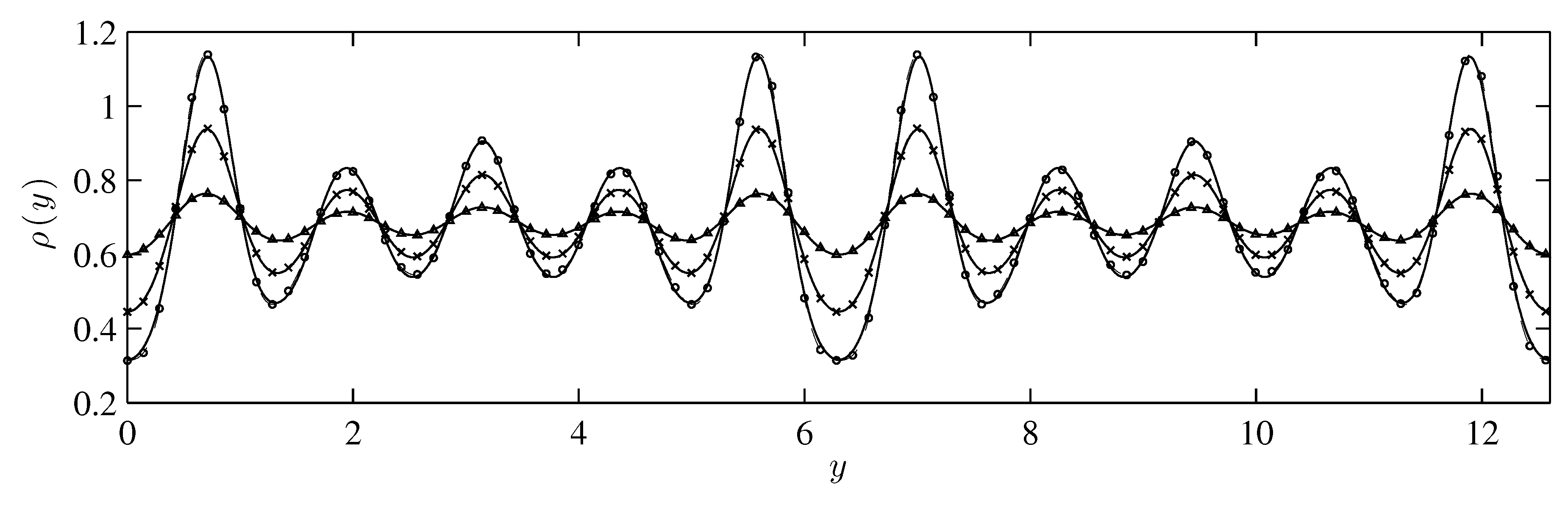
When the longitudinal force responsible for generating density perturbations was extended to a more complicated superposition of sinusoidal components, it was found sufficient to include the longitudinal force components at most coupled in pairs [49]. This is a highly significant result, because it means that considerable simplification is possible. This approach was validated by applying a combination of longitudinal and transverse forces given by
where is the wave number of the STF or SLF, n is a positive integer and and are unit vectors in the x and y directions. By combining these three Fourier components in the SLF, it was possible to construct a non-trivial periodic density profile somewhat resembling the density profiles found in very narrow planar channels, as shown in Figure 7.
With the addition of the transverse force, we can generate flow in a system with strong, and realistically complicated density inhomogeneity. Figure 8 shows the resulting velocity profiles with the predictions obtained from the truncated functional expansion for the velocity gradient. This method is clearly capable of accurately representing the response of a nanoscopic liquid system to a combination of confinement and flow-inducing forces.
6. Conclusions
In this paper, we have provided a brief review of three fundamental phenomena that should be included in an accurate continuum treatment of nanofluidics: slip, spin angular momentum coupling, and non-local response. At the outset, we pointed out that additional complexities would need to be included to account for compositional variation (in binary and multicomponent fluids) and electrostatics, such that a full treatment of ionic solutions and liquids or even polar fluids can be treated. This is clearly some years away. The main complexity is in dealing with the full range of couplings and non-local effects that occur at the nanoscale. A major challenge remains in how to simplify the treatments given in References [46,47,48,49,50] and potentially others not discussed in this brief review such that they can be efficiently applied in predictive nanofluidics. Further advances in the modelling of slip will undoubtedly see the application of both NEMD and EMD methods to complex fluids (e.g., multicomponent mixtures and ionic liquids) and more targeted engineering applications, such as lubrication (see, for example, [51]). The coupling of linear and angular momentum to generate flow poses an intriguing potential application in fluid actuation at the nanoscale. While theoretical and simulation studies exist, there has been no experimental verification to our knowledge.
Author Contributions
P.J.D. and B.D.T. contributed jointly to the conception, supervision and execution of their coauthored work cited in this review. P.J.D. wrote the manuscript, B.D.T. edited and added to it.
Funding
The research undertaken by the authors that has been included in this review was funded by Australian Research Council grant numbers DP0663759 and DP120102976.
Acknowledgments
We would like to acknowledge the contributions made by our collaborators and coauthors to the work reviewed in this article: J.S. Hansen, S.K. Kannam, H. Bruus, S. DeLuca, J.C. Dyre, D. Ostler, F. Frascoli, R. Puscasu, B. Dalton and K. Glavatskiy.
Conflicts of Interest
The authors declare no conflict of interest.
References
- Huilgol, R.R.; Phan-Thien, N. Fluid Mechanics of Viscoelasticity; Elsevier: Amsterdam, The Netherlands, 1997. [Google Scholar]
- Qiao, R.; Aluru, N.R. Atomistic simulation of KCl transport in charged silicon nanochannels: Interfacial effects. Colloids Surf. A Physicochem. Eng. Asp. 2005, 267, 103–109. [Google Scholar] [CrossRef]
- Joly, L.; Ybert, C.; Trizac, E.; Bocquet, L. Liquid friction on charged surfaces: From hydrodynamic slippage to electrokinetics. J. Chem. Phys. 2006, 125, 204716. [Google Scholar] [CrossRef] [PubMed] [Green Version]
- Nilson, R.H.; Griffiths, S.K. Influence of atomistic physics on electro-osmotic flow: An analysis based on density functional theory. J. Chem. Phys. 2006, 125, 164510. [Google Scholar] [CrossRef] [PubMed]
- Schoch, R.B.; Han, J.; Renaud, P. Transport phenomena in nanofluidics. Rev. Mod. Phys. 2008, 80, 839. [Google Scholar] [CrossRef]
- Scarratt, L.R.J.; Steiner, U.; Neto, C. A review on the mechanical and thermodynamic robustness of superhydrophobic surfaces. Adv. Colloid Interface Sci. 2017, 246, 133–152. [Google Scholar] [CrossRef] [PubMed]
- Ho, T.A.; Papavassiliou, D.V.; Lee, L.L.; Striolo, A. Liquid water can slip on a hydrophilic surface. Proc. Natl. Acad. Sci. USA 2011, 108, 16170. [Google Scholar] [CrossRef] [PubMed]
- Hendy, S.C.; Lund, N.J. Effective slip boundary conditions for flows over nanoscale chemical heterogeneities. Phys. Rev. E 2007, 76, 066313. [Google Scholar] [CrossRef] [PubMed]
- Vinogradova, O.I.; Koynov, K.; Best, A.; Feuillebois, F. Direct Measurements of Hydrophobic Slippage Using Double-Focus Fluorescence Cross-Correlation. Phys. Rev. Lett. 2009, 102, 118302. [Google Scholar] [CrossRef] [PubMed] [Green Version]
- Kannam, S.K.; Todd, B.D.; Hansen, J.S.; Daivis, P.J. How fast does water flow in carbon nanotubes? J. Chem. Phys. 2013, 138, 094701. [Google Scholar] [CrossRef] [PubMed]
- Bernardi, S.; Todd, B.D.; Searles, D.J. Thermostating highly confined fluids. J. Chem. Phys. 2010, 132, 244706. [Google Scholar] [CrossRef] [PubMed] [Green Version]
- Kannam, S.K.; Todd, B.D.; Hansen, J.S.; Daivis, P.J. Slip length of water on graphene: Limitations of non-equilibrium molecular dynamics simulations. J. Chem. Phys. 2012, 136, 024705. [Google Scholar] [CrossRef] [PubMed]
- Huang, D.M.; Sendner, C.; Horinek, D.; Netz, R.R.; Bocquet, L. Water Slippage versus Contact Angle: A Quasiuniversal Relationship. Phys. Rev. Lett. 2008, 101, 226101. [Google Scholar] [CrossRef] [PubMed]
- Chinappi, M.; Casciola, C.M. Intrinsic slip on hydrophobic self-assembled monolayer coatings. Phys. Fluids 2010, 22, 042003. [Google Scholar] [CrossRef]
- Bocquet, L.; Barrat, J.L. Hydrodynamic boundary-conditions, correlation functions, and Kubo relations for confined fluids. Phys. Rev. E 1994, 49, 3079. [Google Scholar] [CrossRef]
- Petravic, J.; Harrowell, P. On the equilibrium calculation of the friction coefficient for liquid slip against a wall. J. Chem. Phys. 2007, 127, 174706. [Google Scholar] [CrossRef] [PubMed]
- Kobryn, A.E.; Kovalenko, A. Molecular theory of hydrodynamic boundary conditions in nanofluidics. J. Chem. Phys. 2008, 129, 134701. [Google Scholar] [CrossRef] [PubMed]
- Hansen, J.S.; Todd, B.D.; Daivis, P.J. Prediction of fluid velocity slip at solid surfaces. Phys. Rev. E 2011, 84, 016313. [Google Scholar] [CrossRef] [PubMed]
- Huang, K.; Szlufarska, I. Green-Kubo relation for friction at liquid-solid surfaces. Phys. Rev. E 2014, 89, 032118. [Google Scholar] [CrossRef] [PubMed]
- Chen, S.; Wang, H.; Qian, T.; Sheng, P. Determining hydrodynamic boundary conditions from equilibrium fluctuations. Phys. Rev. E 2015, 92, 043007. [Google Scholar] [CrossRef] [PubMed]
- Kannam, S.K.; Todd, B.D.; Hansen, J.S.; Daivis, P.J. Slip flow in graphene nanochannels. J. Chem. Phys. 2011, 135, 144701. [Google Scholar] [CrossRef] [PubMed]
- Kannam, S.K.; Todd, B.D.; Hansen, J.S.; Daivis, P.J. Interfacial slip friction at a fluid-solid cylindrical boundary. J. Chem. Phys. 2012, 136, 244704. [Google Scholar] [CrossRef] [PubMed]
- Kannam, S.K.; Daivis, P.J.; Todd, B.D. Modeling slip and flow enhancement of water in carbon nanotubes. MRS Bull. 2017, 42, 283–288. [Google Scholar] [CrossRef]
- Yamakawa, H. Modern Theory of Polymer Solutions; Harper and Row: New York, NY, USA, 1971. [Google Scholar]
- Todd, B.D.; Daivis, P.J. Nonequilibrium Molecular Dynamics: Theory, Algorithms and Applications; Cambridge University Press: New York, NY, USA, 2017. [Google Scholar]
- Hansen, J.S.; Dyre, J.C.; Daivis, P.; Todd, B.D.; Bruus, H. Continuum Nanofluidics. Langmuir 2015, 31, 13275. [Google Scholar] [CrossRef] [PubMed] [Green Version]
- Hansen, J.S.; Bruus, H.; Todd, B.D.; Daivis, P.J. Rotational and spin viscosities of water: Application to nanofluidics. J. Chem. Phys. 2010, 133, 144906. [Google Scholar] [CrossRef] [PubMed] [Green Version]
- Hansen, J.S.; Daivis, P.J.; Todd, B.D. Molecular spin in nano-confined fluidic flows. Microfluid. Nanfluid. 2009, 6, 785–795. [Google Scholar] [CrossRef]
- Hansen, J.S.; Dyre, J.C.; Daivis, P.J.; Todd, B.D.; Bruus, H. Nanoflow hydrodynamics. Phys. Rev. E 2011, 84, 036311. [Google Scholar] [CrossRef] [PubMed]
- De Luca, S.; Todd, B.D.; Hansen, J.S.; Daivis, P.J. Molecular dynamics study of nanoconfined water flow driven by rotating electric fields under realistic experimental conditions. Langmuir 2014, 30, 3095–3109. [Google Scholar] [CrossRef] [PubMed]
- Ostler, D.; Kannam, S.K.; Daivis, P.J.; Frascoli, F.; Todd, B.D. Electropumping of Water in Functionalized Carbon Nanotubes Using Rotating Electric Fields. J. Phys. Chem. C 2017, 121, 28158–28165. [Google Scholar] [CrossRef]
- Tanner, R.I. Engineering Rheology, 2nd ed.; Oxford Engineering Science Series; Oxford University Press: New York, NY, USA, 2000. [Google Scholar]
- Puscasu, R.M.; Todd, B.D.; Daivis, P.J.; Hansen, J.S. Viscosity kernel of molecular fluids: Butane and polymer melts. Phys. Rev. E 2010, 82, 011801. [Google Scholar] [CrossRef] [PubMed]
- Dhont, J.K.G.; Kang, K.; Kriegs, H.; Danko, O.; Marakis, J.; Vlassopoulos, D. Nonuniform flow in soft glasses of colloidal rods. Phys. Rev. Fluids 2017, 2, 043301. [Google Scholar] [CrossRef]
- Jin, H.; Kang, K.; Ahn, K.H.; Briels, W.J.; Dhont, J.K.G. Non-local stresses in highly non-uniformly flowing suspensions: The shear-curvature viscosity. J. Chem. Phys. 2018, 149, 014903. [Google Scholar] [CrossRef] [PubMed]
- Todd, B.D.; Hansen, J.S.; Daivis, P.J. Non-local shear stress for homogeneous fluids. Phys. Rev. Lett. 2008, 100, 195901. [Google Scholar] [CrossRef] [PubMed]
- Snook, I.K.; Henderson, D. Monte-Carlo study of a hard-sphere fluid near a hard wall. J. Chem. Phys. 1978, 68, 2134–2139. [Google Scholar] [CrossRef]
- Bitsanis, I.; Magda, J.J.; Tirrell, M.; Davis, H.T. Molecular dynamics of flow in micropores. J. Chem. Phys. 1987, 87, 1733. [Google Scholar] [CrossRef]
- Bitsanis, I.; Vanderlick, T.K.; Tirrell, M.; Davis, H.T. A tractable molecular theory of flow in strongly inhomogeneous fluids. J. Chem. Phys. 1988, 89, 3152–3162. [Google Scholar] [CrossRef]
- Hoang, H.; Galliero, G. Shear viscosity of inhomogeneous fluids. J. Chem. Phys. 2012, 136, 124902. [Google Scholar] [CrossRef] [PubMed]
- Hoang, H.; Galliero, G. Local viscosity of a fluid confined in a narrow pore. Phys. Rev. E 2012, 86, 021202. [Google Scholar] [CrossRef] [PubMed]
- Hoang, H.; Galliero, G. Local shear viscosity of strongly inhomogeneous dense fluids: From the hard-sphere to the Lennard-Jones fluids. J. Phys. Condens. Matter 2013, 25, 485001. [Google Scholar] [CrossRef] [PubMed]
- Bhadauria, R.; Aluru, N.R. A quasi-continuum hydrodynamic model for slit shaped nanochannel flow. J. Chem. Phys. 2013, 139, 074109. [Google Scholar] [CrossRef] [PubMed]
- Bhadauria, R.; Sanghi, T.; Aluru, N.R. Interfacial friction based quasi-continuum hydrodynamical model for nanofluidic transport of water. J. Chem. Phys. 2015, 143, 174702. [Google Scholar] [CrossRef] [PubMed]
- Travis, K.P.; Gubbins, K.E. Poiseuille flow of Lennard-Jones fluids in narrow slit pores. J. Chem. Phys. 2000, 112, 1984. [Google Scholar] [CrossRef]
- Dalton, B.A.; Glavatskiy, K.S.; Daivis, P.J.; Todd, B.D.; Snook, I.K. Linear and nonlinear density response functions for a simple atomic fluid. J. Chem. Phys. 2013, 139, 044510. [Google Scholar] [CrossRef] [PubMed]
- Dalton, B.A.; Daivis, P.J.; Hansen, J.S.; Todd, B.D. Effects of nanoscale inhomogeneity on shearing fluids. Phys. Rev. E 2013, 88, 052143. [Google Scholar] [CrossRef] [PubMed]
- Glavatskiy, K.S.; Dalton, B.A.; Daivis, P.J.; Todd, B.D. Nonlocal response functions for predicting shear flow of strongly inhomogeneous fluids. I. Sinusoidally driven shear and sinusoidally driven inhomogeneity. Phys. Rev. E 2015, 91, 062132. [Google Scholar] [CrossRef] [PubMed]
- Dalton, B.A.; Glavatskiy, K.S.; Daivis, P.J.; Todd, B.D. Nonlocal response functions for predicting shear flow of strongly inhomogeneous fluids. II. Sinusoidally driven shear and multisinusoidal inhomogeneity. Phys. Rev. E 2015, 92, 012108. [Google Scholar] [CrossRef] [PubMed]
- Camargo, D.; de la Torre, J.A.; Duque-Zumajo, D.; Espanol, P.; Delgado-Buscalioni, R.; Chejne, F. Nanoscale hydrodynamics near solids. J. Chem. Phys. 2018, 148, 064107. [Google Scholar] [CrossRef] [PubMed]
- Ewen, J.P.; Kannam, S.K.; Todd, B.D.; Dini, D. Slip of alkanes confined between surfactant monolayers adsorbed on solid surfaces. Langmuir 2018, 34, 3864–3873. [Google Scholar] [CrossRef] [PubMed]
Figure 1.
Schematic diagram showing the flow geometry for the definition of the slip length. The magnitude of the velocity gradient in the fluid at the wall is equal to where is the magnitude of the slip length. Here, we have because we assume flow between stationary walls.
Figure 1.
Schematic diagram showing the flow geometry for the definition of the slip length. The magnitude of the velocity gradient in the fluid at the wall is equal to where is the magnitude of the slip length. Here, we have because we assume flow between stationary walls.

Figure 2.
Calculated relative flow rate reduction between predictions of the Navier–Stokes equations and extended Navier–Stokes equations (including spin angular momentum coupling) for a dumbbell fluid, liquid butane, and liquid water in planar Poiseuille flow. The horizontal axis represents the channel width in units of the Lennard–Jones intermolecular potential parameter . Å and Å for butane and water, respectively. Reprinted with permission from Hansen, J.S.; Dyre, J.C.; Daivis, P.; Todd, B.D.; Bruus, H., Langmuir 31, 13275 (2015). Copyright 2015 American Chemical Society [26].

Figure 3.
Diagram showing rheological flow regimes for typical macroscopic fluids. The horizontal axis represents the degree of elasticity exhibited by the flow, which is controlled by the Deborah number, the product of the characteristic frequency of the flow and the viscoelastic relaxation time of the fluid . The vertical axis represents the degree of nonlinearity of the flow, controlled by the Weissenberg number, the product of the characteristic strain rate and the viscoelastic relaxation time .

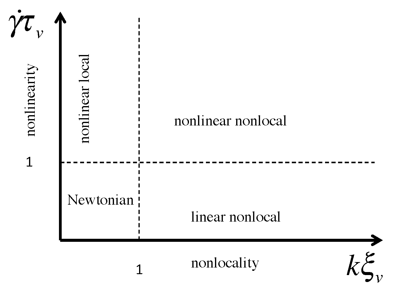
Figure 4.
Diagram showing the rheological flow regimes for fluids exhibiting nonlocal shear pressure response under steady flow conditions. The horizontal axis represents the degree of nonlocality exhibited by the flow, which is controlled by the product of the characteristic spatial frequency (or wavenumber) of the flow k and the viscous correlation length of the fluid . The vertical axis represents the degree of nonlinearity of the flow, controlled by the product of the characteristic strain rate and the viscoelastic relaxation time .

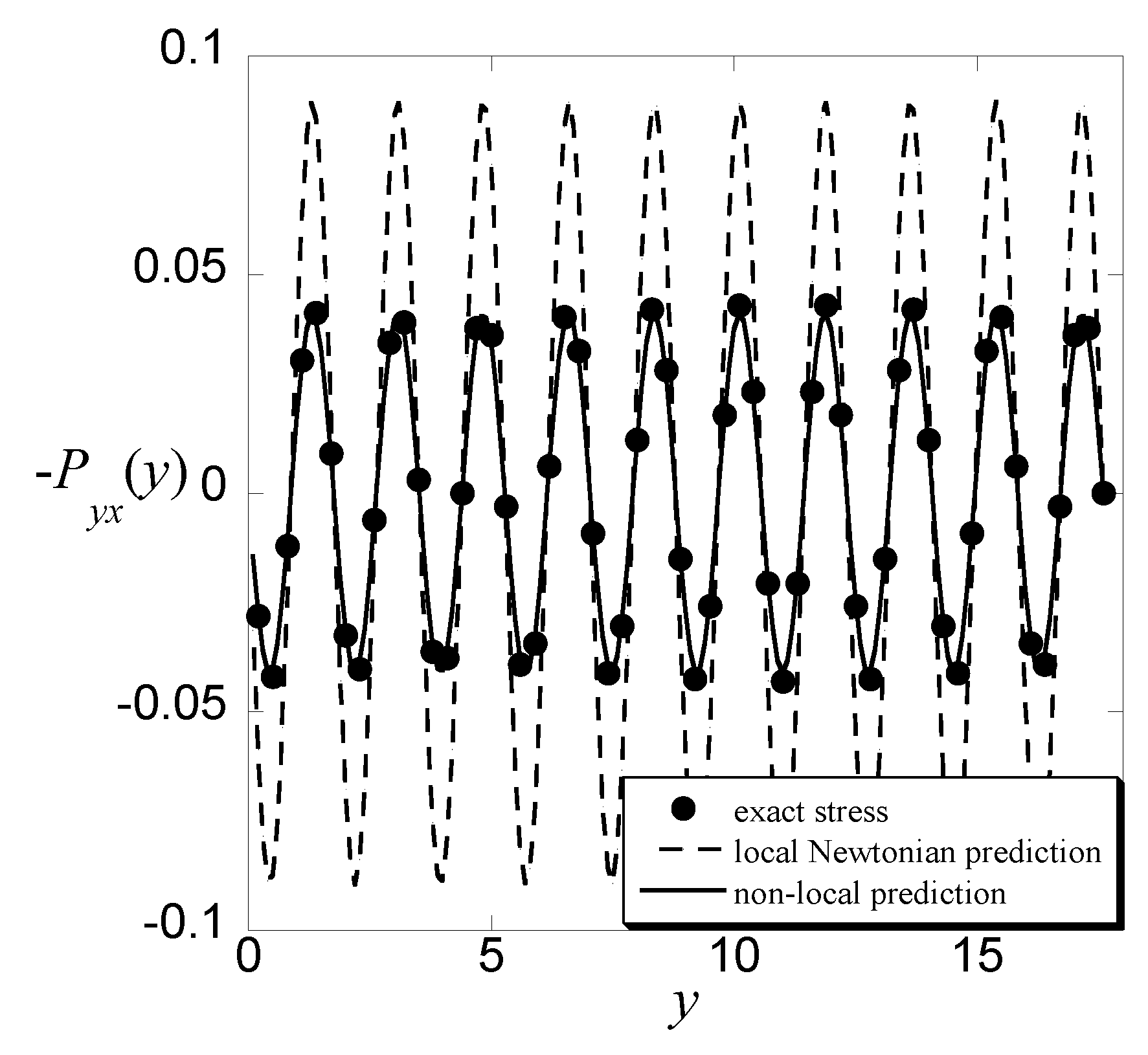
Figure 5.
Shear stress () predictions using the simple Newtonian constitutive equation (dashed line), and the nonlocal constitutive equation (solid line) compared with the exact stress (filled circles) for a simple liquid [36] where the y-position is expressed in units of the Lennard–Jones potential distance parameter .

Figure 6.
Schematic representation of: the sinusoidal transverse force (STF) (a); and the sinusoidal longitudinal force (SLF) (b) fields. The arrows show the direction of the forces. The length of the arrows, as well as the sinusoidal line, indicate the strength of the force. The STF is shown for and the SLF is shown for . Reprinted figure with permission from Glavatskiy, K.S.; Dalton, B.A.; Daivis, P.J.; Todd, B.D., Phys. Rev. E 91, 062132 (2015). Copyright (2015) by the American Physical Society [48].

Figure 7.
Comparison between density profiles obtained directly from MD simulations and the predictions of the truncated functional expansion using previously computed response functions for a three component SLF with , and . Bold lines without symbols represent MD simulations. Thin dashed lines indicated with triangles are for . Thin dashed lines indicated with crosses are for . Thin dashed lines indicated with circles are for . Reprinted figure with permission from Dalton, B.A.; Glavatskiy, K.S.; Daivis, P.J.; Todd, B.D. Phys. Rev. E 92, 012108 (2015). Copyright (2015) by the American Physical Society [49].

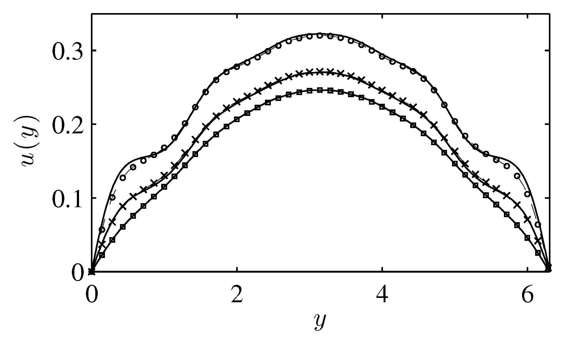
Figure 8.
Comparison between velocity profiles obtained directly from MD simulations and predictions of the truncated functional expansion using independently calculated response functions for a single sinusoidal component STF and a three component SLF. Bold lines represent MD simulations, while thin dashed lines with symbols represent predictions. The system parameters labels are the same as those used in Figure 7. Velocity profiles are only shown for half of a wave cycle. Reprinted figure with permission from Dalton, B.A.; Glavatskiy, K.S.; Daivis, P.J.; Todd, B.D. Phys. Rev. E 92, 012108 (2015). Copyright (2015) by the American Physical Society [49].

© 2018 by the authors. Licensee MDPI, Basel, Switzerland. This article is an open access article distributed under the terms and conditions of the Creative Commons Attribution (CC BY) license (http://creativecommons.org/licenses/by/4.0/).
Share and Cite
MDPI and ACS Style
Daivis, P.J.; Todd, B.D. Challenges in Nanofluidics—Beyond Navier–Stokes at the Molecular Scale. Processes 2018, 6, 144. https://doi.org/10.3390/pr6090144
AMA Style
Daivis PJ, Todd BD. Challenges in Nanofluidics—Beyond Navier–Stokes at the Molecular Scale. Processes. 2018; 6(9):144. https://doi.org/10.3390/pr6090144
Chicago/Turabian StyleDaivis, Peter J., and Billy D. Todd. 2018. "Challenges in Nanofluidics—Beyond Navier–Stokes at the Molecular Scale" Processes 6, no. 9: 144. https://doi.org/10.3390/pr6090144
Note that from the first issue of 2016, this journal uses article numbers instead of page numbers. See further details here.