Population Balance Modeling and Opinion Dynamics—A Mutually Beneficial Liaison?


Technical University of Munich, TUM School of Life Sciences Weihenstephan, Chair of Process Systems Engineering, D-85354 Freising, Germany
*
Author to whom correspondence should be addressed.
Processes 2018, 6(9), 164; https://doi.org/10.3390/pr6090164
Submission received: 16 August 2018
/
Revised: 3 September 2018
/
Accepted: 7 September 2018
/
Published: 11 September 2018
(This article belongs to the Special Issue Recent Advances in Population Balance Modeling)
Abstract
:In this contribution, we aim to show that opinion dynamics and population balance modeling can benefit from an exchange of problems and methods. To support this claim, the Deffuant-Weisbuch model, a classical approach in opinion dynamics, is formulated as a population balance model. This new formulation is subsequently analyzed in terms of moment equations, and conservation of the first and second order moment is shown. Exemplary results obtained by our formulation are presented and agreement with the original model is found. In addition, the influence of the initial distribution is studied. Subsequently, the Deffuant-Weisbuch model is transferred to engineering and interpreted as mass transfer between liquid droplets which results in a more flexible formulation compared to alternatives from the literature. On the one hand, it is concluded that the transfer of opinion-dynamics problems to the domain of population balance modeling offers some interesting insights as well as stimulating challenges for the population-balance community. On the other hand, it is inferred that population-balance methods can contribute to the solution of problems in opinion dynamics. In a broad outlook, some further possibilities of how the two fields can possibly benefit from a close interaction are outlined.
1. Introduction
Population balance modeling (PBM) is a powerful tool to study the dynamics of property-distributed systems. Even though the range of applications is expanding, so far, PBM is mainly used in the engineering and natural sciences to describe particulate systems. For an overview over the theory and applications, we recommend the textbook by Ramkrishna [1] and the recent review by Ramkrishna and Singh [2] as well as the brief historical perspective provided by Sporleder et al. [3]. There have been six “International Conferences on Population Balance Modeling” and four special issues, including this very issue [4,5,6].
However, distributed properties subject to temporal and spatial variations are not only limited to the engineering and natural sciences; they also ubiquitous in the social domain. Examples of such properties are age and income. Another distributed property of interest is individual opinion. Processes of change and formation of public opinion are studied empirically and by means of different modeling approaches in a field called opinion dynamics. In opinion dynamics, other research areas such as social psychology, economics, sociophysics, and complex system science overlap. Contributing researchers also come from mathematics, physics, and computer science [7,8,9].
Studying processes of opinion formation and the influences thereon is motivated by various reasons. For example, human opinion has a direct influence on politics and finance. However, as individual opinion is an important driving force for all human actions, opinion dynamics is indirectly relevant for virtually every topic, from migration to urbanization, from health issues to the environment [8]. Of the various influences on the formation of individual opinion, questions of media, and, especially social media, are currently studied [8,10].
From the characterization provided at the beginning of this section, it follows that there is a big overlap between opinion dynamics and population balance modeling. On the one hand, however, scientists working on opinion dynamics do not seem to be familiar with the theory and methods of population balance modeling even though they deal with populations characterized by distributed properties, e.g., the opinion is not the same for the whole population. On the other hand, the population-balance community is apparently unaware of the interesting application of opinion formation and change. Our thesis, therefore, is that both disciplines can benefit from each other by an exchange of model formulations and solution techniques. To support this thesis, we approach opinion dynamics from a population-balance perspective in this contribution. It is illustrated how solution and analysis methods from PBM can shed new light on opinion-dynamics problems. We also transfer a model formulation from opinion dynamics to engineering to warrant the claim of mutually beneficial effects of an exchange between the two fields. To the knowledge of the authors, this is the first study that establishes an explicit link between opinion dynamics and population balance modeling. Different works that point in a similar direction are highlighted throughout the article.
Different modeling techniques are used in opinion dynamics. In the first place, opinions can be either expressed as discrete or continuous variables. Secondly, either discrete agents are considered or a continuous population of agents is used. The former is referred to as agent-based modeling, the latter as density-based modeling [7]. Some of the most popular models in opinion dynamics are continuous in the opinion but use discrete agents; these models are usually simply referred to as continuous models in the literature. A highly influential approach sharing these characteristics, namely discrete agents and continuous opinions, is the Deffuant–Weisbuch (DW) model [11,12]. The model is widely referred to, extended, or used as a benchmark [7,8]. For example, the DW model was used and analyzed by Urbig et al. [13]. Convergence analyses of different model variants were shown by Zhang and Hong [14], Zhang and Hong [15], and Zhang and Chen [16]. The DW model was even used as a basis for such unconventional applications as image segmentation [17].
In the original formulation of the Deffuant-Weisbuch model, the domain of opinions is . Note that in other formulations also a range from −1 to 1 is used [8]. Perfect mixing is assumed in the simplest model variant, therefore, all discrete agents can interact with all others. Interaction is modeled by pairwise random encounters. As a further item of phenomenological knowledge, the constraint is included that agents only update their opinion upon encounters with others if their original opinions are similar enough, i.e., if their opinions differ in less than some threshold d. This restriction on opinion exchange is referred to as bounded confidence in the literature [7], therefore, d is also called bounded confidence parameter. In other works, d is interpreted as “open-mindedness” [18]. Formally, if the opinions of two agents previous to their encounter are and , they only update their opinion if . This condition being met, the agents adjust their opinions according to
where k is the discrete time step of interactions between agents. is referred to as the convergence parameter and describes how strongly two meeting agents adjust their opinions; it ranges from 0, which corresponds to no change in opinion, to 0.5, which corresponds to both agents having the same opinion after the meeting. The basic procedure of opinion exchange is illustrated in Figure 1. Please note that only the original DW model is presented here. For example, there are similar models which consider an asymmetric d, i.e., the bounded confidence parameter differs if the other agent’s x is smaller or larger [19]. In addition, individual differences in d were investigated [20]. The original DW model only included internal information, i.e., exchange of opinions between equal agents. To overcome this limitation, external information, provided, e.g., by experts or mass media, were also included in some extensions of the model, as reported by Sîrbu et al. [8].
2. Population Balance Model
2.1. Model Formulation
Our reference model, the Deffuant–Weisbuch model, is now reformulated such that it can be expressed as a population balance equation (PBE). In this case, the rate with which agents meet and potentially adapt their opinion is given by
where n is the number density function of agents having opinion x at time t. Note that t is omitted from now on for reasons of brevity.
In the terminology of population balance modeling, we refer to as the opinion exchange rate kernel. It comprises the frequency of encounters and the probability for the encounter to be effective. Corresponding to the DW model from Section 1, is the proportionality constant between the number of meetings and the time ( arbitrarily set to 1 here). Opinion adaption probability can be expressed as
The dependence of on d will be omitted further on in the notation for increased readability. The first condition, as in the original formulation, excludes adaptation of opinions that are too different from each other. Obviously, many other formulations are conceivable from non-constant frequency of encounters to much more elaborate opinion adaptation probabilities.
An effective encounter of two agents of opinion and shifts the opinions of the respective agents according to:
Note that, in order to form a new opinion x from an encounter with an agent with opinion , the interacting agent needs to have one of the two following complementing opinions and , respectively. This complementing opinion is obtained by solving Equations (5) and (6) for with the left hand side () set to x:
The resulting population balance formulation comprises one sink term and one source term:
Equation (9) is derived in detail in Appendix A and is only explained here. One can observe some differences to conventional PBE formulations from chemical engineering. The source term is not divided by two because two agents emerge again after each interaction event. An exchange of opinions between two agents creates two new opinions that are both in between the original ones. Therefore, the integration cannot be limited to the interval , but rather is limited to the more complicated domain . Figure A1 in the appendix provides an illustration of this modified domain. We use the somewhat unusual formulation of the PBM as a warrant for our claim that problems in opinion dynamics also offer new perspectives to the formulation and simulation of population balances. In Section 4, we provide an example of such an opinion dynamics-inspired model formulation concerning mass transfer, i.e., concentration exchange, between liquid droplets.
It is important to mention that a similar continuous formulation of the DW model was presented by Lorenz [7] where the equation, however, was not interpreted as a population balance. Even more importantly, Toscani [21] and Boudin and Salvarani [22] approached opinion dynamics from a PBM-like perspective. They took the DW model as a starting point and reformulated it as an equation similar to the Boltzmann equation. As Marchisio and Fox [23] showed that the Boltzmann equation is a PBE if the number of particles is sufficiently high, one could count the work by Toscani [21] as the first formulation of opinion dynamics in a PBM-like framework. The reader is also referred to newer work by Boudin et al. [24,25]. However, the latter authors also neither explicitly interpret their models as PBMs nor perform the following analyses.
2.2. Initial Distribution
In 2007, Lorenz [7] observed that most studies relied on initially uniformly distributed opinions. He stated the importance of the initial opinion distribution on opinion formation and declared it as a promising subject for future work. In the meantime, different research has addressed this question. Some authors included non-uniform initial distributions in agent-based simulations [8,26]. Shang [27] derived a critical threshold of the bounded confidence parameter for which opinions converge toward the average value of the initial opinion distribution, provided the initial distribution has a finite second order moment. He also used agent-based simulations for uniform, beta, power-law, and normal distributions, and showed a faster convergence behavior for unimodal initial distributions. Recently, Antonopoulos and Shang [28] investigated the influence of bounded confidence and initial opinion distribution analytically and numerically by agent-based simulations. They especially stressed the importance of the interaction between these two factors.
We continue the analysis of the influence of initial opinion distributions on consensus formation along similar lines. However, our method is based on the population-balance formulation presented in Section 2.1 which allows for different analysis methods compared to the literature just cited. In the present study, the beta distribution is used to characterize the initial distribution because it is only defined on and can be completely characterized in terms of the initial variance and the initial mean [29]. With and , the beta distribution can represent a uniform distribution. For decreasing values of the variance, it approaches a peak at 0.5, and for higher values of the variance, it yields an initially polarized population with beliefs of 0 and 1 only.
2.3. Model Analysis
As a first analysis, the PB formulation of the DW model is formally analyzed in terms of moments. As the total number of agents has to be conserved, visual inspection of the model equations can lead to the conjecture that also the total belief B is conserved. This hypothesis is underpinned by rigorous analysis, as shown in Appendix B. It is proven that the zeroth and first moment indeed stay constant for the basic DW model. The same results were also observed by Lorenz [7] and Ben-Naim et al. [30]. However, these authors did not show it by rigorous analysis but concluded it from the dynamic updating rules. On the contrary, Toscani [21] proved the conservation of total belief B for the special case in which all agents can interact with each other. Additionally, it should be mentioned that a constant B is not a necessary property of all opinion-dynamics models. For example, the Hegselmann-Krause model [19], another standard opinion-dynamics model which is in other respects quite similar to the DW model, does not have this property [7].
An analysis of the second order moment allows insights about the variance, as shown in Appendix B. First of all, an analytical solution for the variance is derived for . Therefore, for this special case, numerical simulations are only necessary to obtain the full distribution. Subsequently, it is shown that the variance monotonically decreases for any . This implies that, if the distribution changes, it always changes towards a local consensus. The same behavior has been observed by Ben-Naim et al. [30] and Lorenz [7], but has not been proven in these studies. A notable exception is the work of Toscani [21] which provides a similar proof as presented in the appendix, although his analysis was again only performed for the special case where all agents can interact with each other. However, as such methods are still very rarely used in opinion dynamics, we use our conducted moment analysis as evidence for the thesis that PBM methods offer new ways of thinking about and analyzing problems in opinion dynamics.
2.4. Numerical Methods
All computations were performed with MATLAB (version: 2017b, supplier: The MathWorks, Natick, MA, USA). The continuous PBE was discretized using the Fixed Pivot technique [31]. A mesh with 201 pivots at the position with was used. The system of ordinary differential equations (ODE) was solved using the MATLAB-integrated ODE-solver ode23t with an equal relative and absolute tolerance of 1 × 10⁻⁶ and the analytically computed Jacobian matrix. In Appendix B.7, it is shown that for at least one case () the steady state distribution is reached in infinite time. This makes it impossible to simulate until the system reaches the steady state. Therefore, the simulations were run for at least 1000 time units and until the norm of the derivative with respect to time was less than 1 × 10⁻⁷. From this almost steady state, the steady state was estimated. Peaks were identified as clusters with the amount of agents at a pivot never less than 1 × 10⁻⁶. The number of agents in these clusters and their mean belief was computed. From this, the variance in the estimated steady steady was computed. This variance is almost identical to the variance computed from the distribution at the end of solving the ODEs. Accordingly, the state at the end of solving the ODEs should be sufficiently close to the steady state.
3. Numerical Results
Some exemplary results obtained by our PBE formulation of the DW model are shown in this section. First, we focus especially on the influence of the convergence parameter and the bounded confidence parameter d for an initially uniform opinion distribution. In a second step, the influence of the initial distribution is also studied.
3.1. Uniform Initial Distribution
Figure 2a shows the evolution of the initially uniform opinion distribution over time for and . Note that the uniform distribution corresponds to a beta distribution with mean belief equal to 0.5 and a variance of . It can be observed that all opinions converge over time to a value of , i.e., all individuals settle on the mean opinion.
Decreasing the value of from 0.5 to 0.1 leads to the same steady state but with different dynamics and different intermediate states, as shown in Figure 2b. This is well in agreement with the nomenclature of the parameter, and it was also observed in the literature that only influences the dynamics but not the steady state [7].
In contrast, the steady state is strongly influenced by the bounded confidence parameter d, as shown in Figure 3a,b. It can be seen that the number of peaks increases with decreasing bounded confidence. Whereas with , as shown in Figure 2a, all individuals could interact with each other, smaller d values result in a decreased interaction behavior which influences the steady state. It was also observed that the number of the forming opinion clusters c for uniformly distributed initial opinion can be approximated as [8,18]
which is in good agreement with our simulation results. For (see Figure 2a,b) and (see Figure 3b), our simulations yield one and five clusters, which is also predicted by Equation (10). For (see Figure 3a), we obtain three clusters, whereas Equation (10) predicts four clusters. Almost no agents, however, are represented by cluster three at . Therefore, the Monte Carlo approach used to derive Equation (10) [8,18] might not have resolved the unlikely event of agents having this belief.
The shown qualitative as well as the quantitative results are well in agreement with the original publications of the DW model [11,12] as well as with the further model uses cited above. We, therefore, conclude that our implementation of the PBM is a suitable equivalent to the original agent-based form of the DW model.
3.2. Influence of Initial Distribution
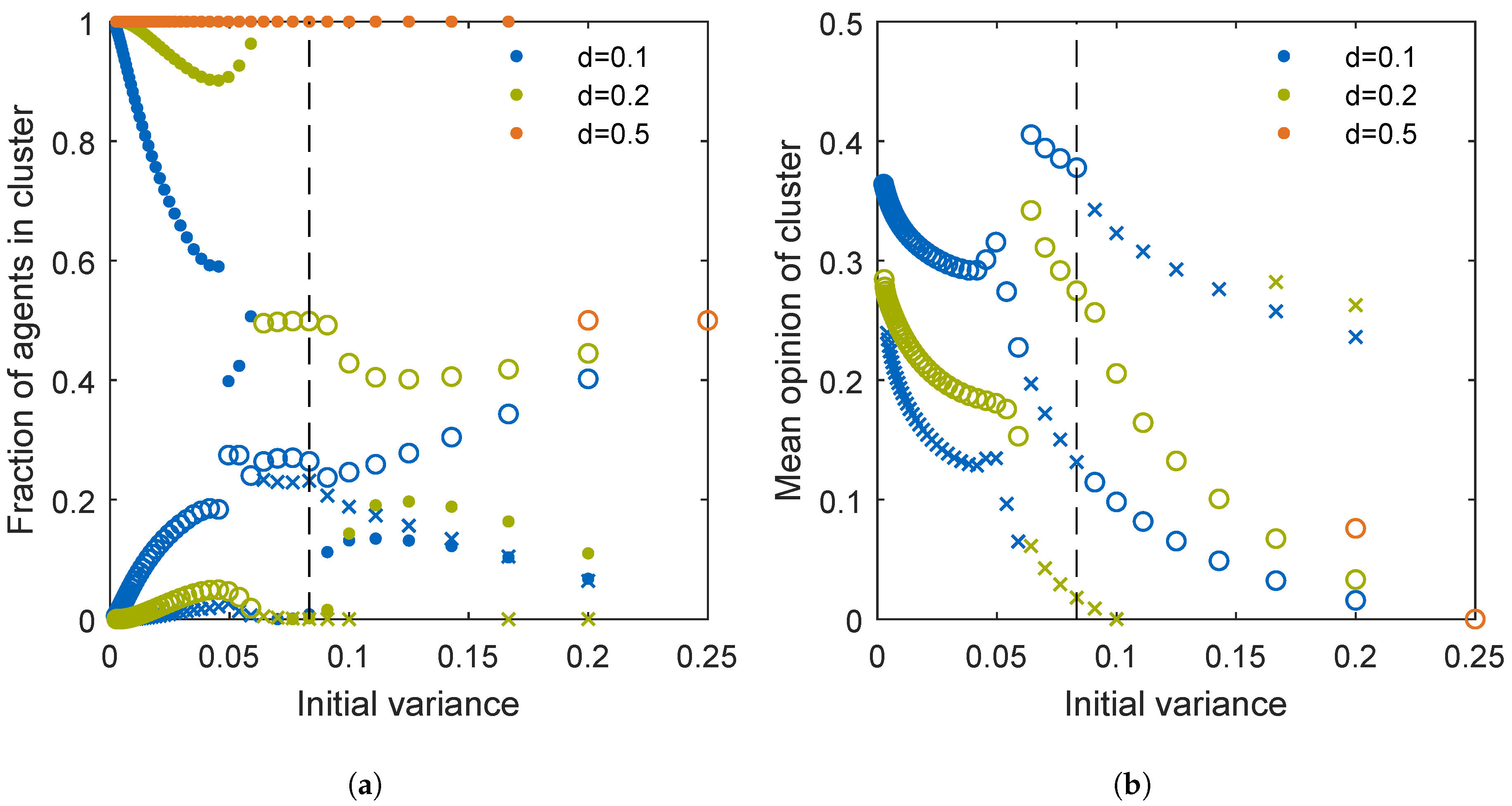
The initial distribution is plotted for several values of the variance and a mean opinion of 0.5 in Figure 4a. The resulting variance of the steady state distribution is shown in Figure 4b for three different values of d. Unless d is equal to 1, the variance stays constant for an initial value of 0.25, which corresponds to a population completely polarized into two radical opinions at 0 and 1. For , the steady state variance becomes 0 for initial variances less than 0.2, which means that the steady state distribution has just a single peak, if the steady state distribution is not too strongly polarized into two radical extremes. The variance goes slowly to 0 for smaller values of d. Thus, only for initially low dispersions of opinion does the distribution converge to one opinion. The fraction of agents in clusters of the steady state distribution is shown in Figure 5a, and the corresponding mean opinion of the clusters is presented in Figure 5b. Because the distribution is symmetric around 0.5, only the clusters with an opinion of less than 0.5 are shown. For , the distribution has only one cluster at 0.5 for all variances less than 0.2. For a variance of 0.2, there are two clusters: one with half the agents at 0.076 and mirrored at 0.924. For , almost all agents are within three clusters: one at the center, and two closer to the extreme opinion. If the variance is decreased, these two clusters move closer to the center. Close to an initially uniformly distributed belief, (almost) no agents have a belief of 0.5, as was shown in Figure 3a. If the initial variance decreases below , the number of agents in the cluster at 0.5 increases suddenly and the remaining clusters are closer to the extreme beliefs. With a decrease in initial variance, the fraction of agents in the central cluster increases and the initial clusters converge to the cluster in the center. There are more clusters than the clusters discussed here, but almost no agents are represented by them. For , there are at least five clusters: one at 0.5 and the other four closer to the extreme opinion. Again, the importance of the central cluster increases, until close to an initially uniformly distributed belief for which the central cluster becomes relatively unimportant, as can be seen in Figure 3b. For smaller variances, the central cluster becomes dominant and the remaining clusters diminish in fraction of agents and move closer to the center.
4. Transfer to Engineering
The presented opinion dynamics models, formulated as PBEs, may also provide useful grounds for approaching chemical-engineering phenomena that to our knowledge have not been addressed in a detailed manner yet. One such phenomenon could be liquid-liquid disperse systems undergoing coalescence and breakage, including mass transfer between colliding droplets. We use this example to show how the DW model can be given a process-engineering interpretation which provides a novel description of the said behavior. This in turn supports our claim that the PBM community can also benefit from an exchange with opinion dynamics.
There is a large number of population balance-related work on the formation of emulsions, e.g., [32]. One is typically interested in the evolution of the droplet size distribution which is governed by the hydrodynamic conditions inducing breakage and coalescence terms. If, however, the emulsion droplets have a specific concentration, one may immediately end up with at least a two-dimensional problem. This is prominently the case for liquid-liquid extraction columns [33,34]. There, the coalescence and breakage not only affects droplet sizes but additionally leads to mass transfer by temporarily coalesced droplets. It is, however, implicitly assumed that the concentration exchange is much faster than the time scale of coalescence and breakage. Though this may be the case for many applications, the given opinion dynamics framework presents the means to easily avoid this assumption. In a case where coalescence and breakage may be very fast but concentration exchange might be hindered, it is easily conceivable that the droplet size reaches a dynamic equilibrium quickly. Then, the concentration exchange within colliding droplets is no longer complete, but the concentration evolves according to the frequent coalescence and breakage events. The only characterizing variable of the emulsion droplets then is the concentration.
Another example is the use of microdisperse systems as microreactor systems, e.g., employed for nanoparticle preparation. In the so-called two-emulsion methods, two emulsions with different composition, typically one precursor in a solvent in each of the two emulsions, are mixed by coalescence (and potentially breakage) followed by a reaction/precipitation within the droplet [35]. Apart from the many experimental studies, see Niemann et al. [36] and references therein, there are some studies using population balance concepts to address various aspects of the corresponding process. As the goal of the process eventually is the formation of nanoparticles, most studies aim towards the prediction of the particle formation, e.g., [37]. Hatton et al. [38] proposed a population dynamics framework that considered different modes of concentration exchange after coalescence, namely random, cooperative, and repulsive distribution. While in the cooperative and repulsive exchange mode, the exchange is affected (promoted/hindered, respectively) by the presence of the already formed solute molecules or nanoparticles, the random mode considers unaffected exchange. Several aspects of the process have been studied by stochastic simulations. Natarajan et al. [39] Bandyopadhyaya et al. [40] Kumar et al. [41] as well as Jain and Mehra [42] assume complete mixing of coalescing droplets followed by redistribution of the reactants and products. In some cases, the size of the droplets is in the order of nanometers. Then, the very low number of precursor molecules leads to a discrete characterizing variable for the population balance formulation, e.g., [43]. Also, the effect of micromixing within the droplets has been studied in a population-balance framework [44].
The analogy of these disperse systems to the above introduced opinion-dynamics framework is largely apparent. Instead of opinion adaptation of individuals, there is a concentration adaptation of droplets upon encounter. Similar as opinions not having to settle on a common opinion, neither does the droplet concentration have to become fully equilibrated. Of course, dispersity in size of the droplets could directly be implemented in the scheme yielding a multi-variate population balance formulation. Here, we only use a simple scenario to illustrate such emulsion mixing processes without considering any further reaction to show the analogy to the opinion dynamics case. The initial state comprises two different types of emulsions for which the total volume fraction of each emulsion phase is and , respectively. The two initial emulsion phases are distinguished by their initial concentration of the two precursors A or B only.
We use a non-dimensional concentration measure to be able to directly employ the opinion dynamics framework presented above. A dynamic steady state with respect to droplet size is assumed. Considering the molar concentrations in the constant single-droplet volume V as and , respectively, the chosen concentration measure uniquely characterizing an arbitrary droplet is
Adapting the formulations to other concentration measures is straightforward. Droplets undergo permanent coalescence and immediate breakage at a certain rate , depending on the prevailing hydrodynamic conditions. In contrast to opinion dynamics, it is less plausible that there are coalescence/breakage events that do not at all lead to a concentration exchange. Thus, the bounded confidence parameter can be set to unity. However, depending on the hydrodynamics, the concentration exchange may vary. Similar to above, the convergence parameter reflects this behavior. can be given a physical meaning in this case: if one imagines that with one collision only a certain volume is exchanged and, in turn, perfectly mixed within both interacting droplets, then the convergence factor is this volume divided by twice the total volume. The basic procedure of concentration exchange is illustrated in Figure 6. Note that this process, given the above concentration measures and model assumptions, is described by the very same equation as used in the DW model, namely Equation (9).
Using the initial condition,
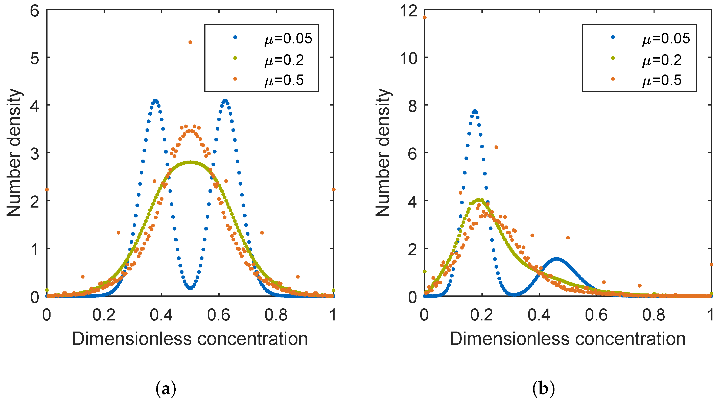
results in the initial mean and the initial variance . The time evolution of the variance is given by Equation (A29) in the appendix. The parameter , therefore, controls the speed of decay of the variance. We simulated the time evolution of the system for several values of and . The results for three values of are shown in Figure 7a,b. In order to compare the results in these figures, the times were selected such that all three curves have the same variance. One can see that variance is not sufficient to describe the state. Furthermore, even for two colliding droplets having equal concentration afterwards (), not all droplets have the same concentration. The skewness of the distribution [45] was computed (data not shown), and the concentration exchange decreases the skewness towards zero. The distribution of the concentration is also important, if a nonlinear reaction occurs, because the reaction in each droplet would depend on the concentration of A and B in the droplet, as it has already been highlighted in the study by Singh and Kumar [44]. If a reaction occurs, then no analytical solution for the variance is known and one would have to solve the PBE numerically.
5. Conclusions
In this contribution, we presented opinion dynamics as an interesting application for the use of PBM methods. To illustrate this case, the Deffuant-Weisbuch model, a classical approach in the field of opinion dynamics, was introduced and reformulated as a PBE. Exemplary results were shown and agreement to results from literature was observed. Furthermore, we analyzed our PB formulation of the DW model to prove that total belief is conserved. It was also proven for the first time that the variance monotonically decreases for all values of the bounded confidence parameter larger than zero. This implies that, if the distribution changes, it always changes towards a local consensus. As analyses of this type are still very rarely used in opinion dynamics, we use this observation to underpin our thesis that PBM methods offer new ways of approaching and analyzing problems in opinion dynamics.
It must be highlighted, however, that this contribution is not the first work that approaches opinion dynamics from a PBM-like perspective. As already mentioned earlier in the text, the reader is explicitly referred to work by Boudin and Salvarani [22,24,25] as well as Toscani [21] and Lorenz [7,20]. However, in the opinion of the authors, this is the first contribution where an explicit connection between PBM and opinion dynamics is made and possible benefits of an exchange between these two fields are asserted.
To warrant the claim that there are indeed mutually beneficial effects, as suggested by the title of this article, a transfer of the opinion-dynamics approach to engineering was formulated for the example of concentration exchange between monosized droplets. It was illustrated that this scenario can be described by the same formulation as used in the Deffuant-Weisbuch model, given suitable model assumptions and concentration measures. Besides the shown example of concentration exchange, also tribolelectric charging of particles can be mentioned as a similar application. In this case, insulating particles exchange and also generate electric charge due to inter-particle collisions. Usually, the particle sizes remain constant during this process. The similarity to opinion dynamics lies in the modification of a given property of single elements, here their electrical charge, upon contact with other elements [46,47].
Besides these possible benefits for the formulation of novel models, some further, more methodological, advantages of an exchange between PBM and opinion dynamics are outlined now. PBM can offer a flexible and efficient computational framework for the field of opinion dynamics. Especially continuous PBMs have the benefit of a high computational efficiency compared to the agent-based modeling techniques that are mostly used so far in the field of opinion dynamics. Computational efficiency, in turn, is an important prerequisite for further model uses such as parameter estimation and optimization. For example, Sîrbu et al. [8] stated the importance of model validation with empirical data as an important topic for future work in opinion dynamics. The community might, therefore, benefit from efficient parameter estimation strategies that are available for continuous PBMs. Additionally, multidimensional problems are often encountered in classical PB research and various solution strategies are known. In a similar manner, one can easily imagine corresponding multidimensional problems in opinion dynamics [8], e.g., systems that are distributed in opinions on different subjects or in opinion, age, and income, to pick up the example from the introduction. Such multidimensional problems would, thus, benefit from the knowledge and methods available in the PBM community. Furthermore, PB can easily be coupled with other transport equations. In this manner, it is straightforward to move from perfectly mixed systems to more realistic scenarios of opinion exchange. The use of PBM could, therefore, foster new developments in opinion dynamics. However, not only the field of opinion dynamics can benefit from PBM. The PBM community might also benefit from a completely new and different application. The new problems posed by opinion dynamics require new formulations for the corresponding birth and death terms which might, in turn, cause specific numerical challenges and, therefore, encourage extension and modification of existing numerical methods. In summary, we suggested to extend the application of PBM also to the social domain and showed that opinion dynamics is a very promising candidate for such a transdisciplinary endeavor.
Author Contributions
M.K. provided the research idea, conceptualized the work, and wrote the initial draft of the article; C.K. and H.B. conducted the model analysis; C.K. performed all simulations; H.B. conceived of the transfer back to engineering, i.e., the concentration-exchange model; C.K., H.B. and M.K. discussed and interpreted the results and wrote the final paper.
Funding
This research received no external funding.
Conflicts of Interest
The authors declare no conflict of interest.
Abbreviations
The following abbreviations are used in this manuscript:
| DW model | Deffuant-Weisbuch model |
| PB | population balance |
| PBE | population balance equation |
| PBM | population balance model |
Appendix A. Derivation of Population Balance Equation
A detailed derivation of the model formulation discussed in Section 2.1 of the main text is presented in this appendix. The rate with which two agents meet is given by Equation (3). If two agents interact, they adapt their opinion according to Equations (5) and (6). Thus, by multiplying the meeting rate with a sum of two Dirac deltas one can obtain the rate of two agents with opinion and producing an agent with opinion x (either by adaption from or ). If one integrates over all possible encounters (over all and ), one obtains the rate of generating agents with opinion x
The terms in the Dirac delta can be expressed in terms of (see Equation (7)). Additionally, the integral is split in two parts and is taken out of the integrals:
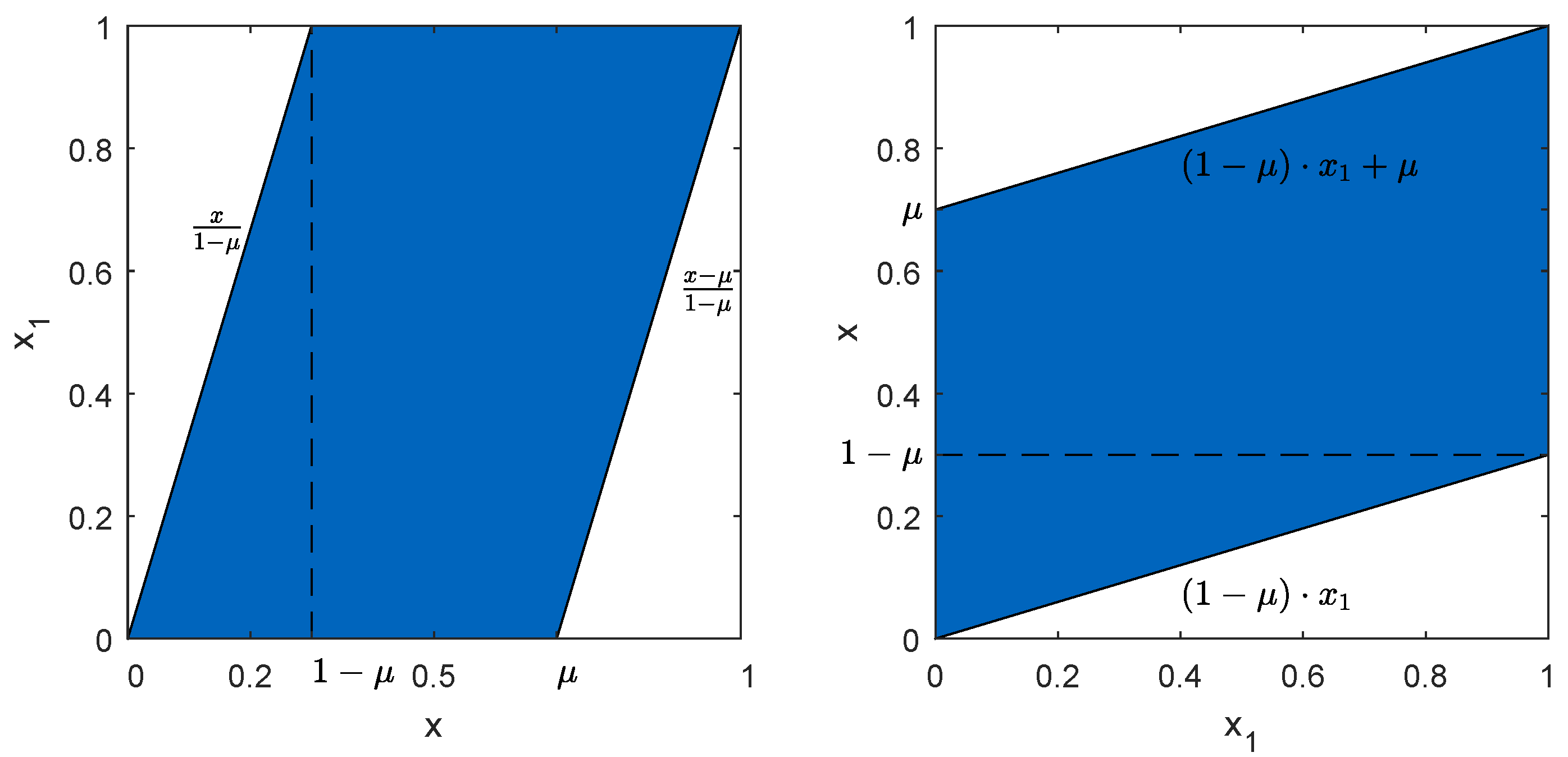
Not all values of x and produce a valid complement that is a complement within the domain . If the complement is not valid, the Dirac delta will be zero and, therefore, limiting the outer integral limits to only producing valid complements does not change the value of the integral. Solving the two linear inequalities and leads to the linear inequalities and . Furthermore, , which leads to the admissible domain for shown in Figure A1. The limits of integration for the outer integral of the first term are thus . Switching the order of integration for the second term allows using the same argumentation yields
Figure A1.
Region of x and that results in a valid complement ; for illustration purposes, was set to 0.7.
Figure A1.
Region of x and that results in a valid complement ; for illustration purposes, was set to 0.7.

Now using the sifting and scaling property of the Dirac delta [48], the inner integrals can be evaluated:
Because and , the two integrals are the same and only one integral is required:
Having clarified the production term, one can use the sink term from Ramkrishna [1] and write the PBE in the final form
Appendix B. Moment Analysis
In this appendix, the moment analysis referred to in Section 2.3 of the main text is explained in detail. First, some definitions are made. Then, it is shown that the total number of agents and the total belief stays constants. Subsequently, the solution for the variance for is derived. Finally, it is shown the variance monotonically decreases for an arbitrary d.
Appendix B.1. Definition of Moments
The i-th order moment is defined as
The zeroth order moment is the total amount of agents. The first order moment is the total belief B. According to Pruim [45], the variance can be computed from the second, first, and zeroth order moment:
Appendix B.2. Transformation to a Square Integration Domain for the Source Term
In Figure A1, the region of x and that yields a valid complement is shown. If one looks at the right side, one can see that, given a , the linear inequalities for the valid x that result in a are simpler. They are . The integral of any function over the blue region in Figure A1 can thus be stated in two ways:
Switching the order of integration leads to a more straightforward integral. A further simplification is possible, if one transforms the inner integration variable x to . The transformed limits of integration are then
Thus, if one integrates over the complements, the integration is performed over the unit square. The value of x corresponding to and is given by Equation (5). Changing the integration variable leads to a scaling:
Thus, the integral over f can be written as
Appendix B.3. Derivation of Ordinary Differential Equation for the Moments
Multiplying the PBE with and integrating over the domain yields an ordinary differential equation for the i-th order moment because integration with respect to x and differentiation with respect to time can be exchanged:
Following the same procedure as in Appendix B.2 for the source integral leads to
Appendix B.4. Constant Number of Agents
For the zeroth order moment , the source integral simplifies to
As this is equal to the sink term of Equation (A14), the equation for the evolution of the total number of agents N is
Therefore, the total number of agents stays constant as expected.
Appendix B.5. Constant Total Belief
For the first order moment , the source term (Equation (A15)) becomes
If one switches the order of integration, one obtains
Because is symmetric, the inner integrals will have the same value and the double integrals are equal. Thus, the sum of both is equal to the sink term of Equation (A14). The equation for the total belief is then
Therefore, the total belief stays constant.
Appendix B.6. Ordinary Differential Equation for the Variance
For the second order moment , which results in the following formulation for the source term:
By using binominal expansion, this can be rewritten as
As the order of integration can be switched and the is symmetric, one can include the first double integral in the third
Subtraction of the sink term yields the prefactor for the second term. Thus, the second order moment evolves according to
Because the zeroth and first order moments are constant, the derivative of the variance is equal to the derivative of the second order moment divided by the zeroth order moment (see Equation (A8)):
Appendix B.7. Exponential Decay of Variance for d = 1
If one considers the case with , which implies that is always equal to one, then the ordinary differential equation for can be simplified to
Utilizing the definition of the variance (Equation (A8)), one obtains the final form:
Thus, the variance decays exponentially for , if :
Appendix B.8. Variance for an Arbitrary d
The next goal is to show that monotonically decreases for and , i.e.,
If and only if the initial distribution is a Dirac delta, the initial variance is equal to zero. In this case, the initial distribution does not change and the variance stays zero:
Thus, Equation (A30) is always satisfied, if the initial variance is equal to zero. The case with an initial variance of zero is, therefore, excluded from the further discussion. For , it was derived that decreases exponentially with time:
If one considers the case with , which implies that is always equal to zero, then the right-hand side is equal to zero and the variance is constant:
If the derivative of the right-hand side of Equation (A26) with respect to d is always non-positive, the variance has to monotonically decrease in the interval as it has been already shown for the borders:
The derivative of the right-hand side of Equation (A26) is
For , the constant term . We, therefore, focus on the double integral and aim to show that this integral is non-positive:
Because (see Equation (4)) depends only on d and the difference between x and and not x or , one can introduce the variable and a simpler expression for in terms of this variable:
Using this function and the transformation allows rewriting the integral (see Equation (A36)) as
The derivative of with respect to d is
Using the sieving property of the Dirac delta, the first inner integral becomes
Substituting this into the double integral and changing the limits of the outer integral allows writing a simpler form
A similar argument permits expressing the second double integral as
Introducing the substitution , the equation can be further simplified:
Because , the remaining integral is always greater than or equal to zero. Furthermore, unless n consists out of Dirac deltas at least d apart, the remaining integral is greater than zero. Thus, the derivative of the right-hand side of Equation (A26) is always less than (or equal to for Dirac deltas at least d apart) zero and the derivative of with respect to time is always less than (or equal to for Dirac deltas at least d apart) zero. If n consists out of Dirac deltas at least d apart, the time derivative of n is zero. Thus, if n changes, it always evolves towards a (local) consensus.
References
- Ramkrishna, D. Population Balances; Academic Press: London, UK, 2000. [Google Scholar]
- Ramkrishna, D.; Singh, M.R. Population Balance Modeling: Current Status and Future Prospects. Annu. Rev. Chem. Biomol. Eng. 2014, 5, 123–146. [Google Scholar] [CrossRef] [PubMed]
- Sporleder, F.; Borka, Z.; Solsvik, J.; Jakobsen, H.A. On the population balance equation. Rev. Chem. Eng. 2012, 28, 149–169. [Google Scholar] [CrossRef]
- Nopens, I.; Biggs, C. Advances in population balance modelling. Chem. Eng. Sci. 2006, 61, 1–2. [Google Scholar] [CrossRef]
- Nopens, I.; Briesen, H.; Ducoste, J. Celebrating a milestone in Population Balance Modeling. Chem. Eng. Sci. 2009, 64, 627. [Google Scholar] [CrossRef]
- Kumar, S.; Briesen, H. Population balances in the league of mass, momentum, and energy balances. Chem. Eng. Sci. 2012, 70, 1–3. [Google Scholar] [CrossRef]
- Lorenz, J. Continuous Opinion Dynamics under Bounded Confidence: A Survey. Int. J. Mod. Phys. C 2007, 18, 1819–1838. [Google Scholar] [CrossRef]
- Sîrbu, A.; Loreto, V.; Servedio, V.D.P.; Tria, F. Participatory Sensing, Opinions and Collective Awareness. In Participatory Sensing, Opinions and Collective Awareness; Loreto, V., Haklay, M., Hotho, A., Servedio, V.D., Stumme, G., Theunis, J., Tria, F., Eds.; Chapter Opinion Dynamics: Models, Extensions and External Effects; Springer: Cham, Swizerland, 2017; pp. 363–401. [Google Scholar]
- Schweitzer, F. Sociophysics. Phys. Today 2018, 71, 40–46. [Google Scholar] [CrossRef]
- Gargiulo, F.; Lottini, S.; Mazzoni, A. The saturation threshold of public opinion: Are aggressive media campaigns always effective? arXiv, 2008; arXiv:0807.3937. [Google Scholar]
- Deffuant, G.; Neau, D.; Amblard, F.; Weisbuch, G. Mixing beliefs among interacting agents. Adv. Complex Syst. 2000, 3, 87–98. [Google Scholar] [CrossRef]
- Weisbuch, G.; Deffuant, G.; Amblard, F.; Nadal, J.P. Interacting Agents and Continuous Opinions Dynamics. In Heterogenous Agents, Interactions and Economic Performance; Cowan, R., Jonard, N., Eds.; Springer: Berlin/Heidelberg, Germany, 2003; pp. 225–242. [Google Scholar]
- Urbig, D.; Lorenz, J.; Herzberg, H. Opinion Dynamics: The Effect of the Number of Peers Met at Once. J. Artif. Soc. Soc. Simul. 2008, 11, 4. [Google Scholar]
- Zhang, J.; Hong, Y. Convergence analysis of heterogeneous Deffuant–Weisbuch model. In Proceedings of the 31st Chinese Control Conference, Hefei, China, 25–27 July 2012; pp. 1124–1129. [Google Scholar]
- Zhang, J.; Hong, Y. Convergence Analysis of the Long-range Deffuant–Weisbuch Dynamics. IFAC Proc. Vol. 2013, 46, 141–146. [Google Scholar] [CrossRef]
- Zhang, J.; Chen, G. Convergence rate of the asymmetric Deffuant–Weisbuch dynamics. J. Syst. Sci. Complex. 2015, 28, 773–787. [Google Scholar] [CrossRef]
- Kayal, S. Unsupervised image segmentation using the Deffuant–Weisbuch model from social dynamics. Signal Image Video Process. 2017, 11, 1405–1410. [Google Scholar] [CrossRef]
- Carletti, T.; Fanelli, D.; Grolli, S.; Guarino, A. How to make an efficient propaganda. Europhys. Lett. 2006, 74, 222. [Google Scholar] [CrossRef]
- Hegselmann, R.; Krause, U. Opinion dynamics and bounded confidence: Models, analysis and simulation. J. Artif. Soc. Soc. Simul. 2002, 5, 1–24. [Google Scholar]
- Lorenz, J. Heterogeneous bounds of confidence: Meet, discuss and find consensus! Complexity 2010, 15, 43–52. [Google Scholar] [CrossRef]
- Toscani, G. Kinetic models of opinion formation. Commun. Math. Sci. 2006, 4, 481–496. [Google Scholar] [CrossRef] [Green Version]
- Boudin, L.; Salvarani, F. A kinetic approach to the study of opinion formation. Math. Model. Numer. Anal. 2009, 43, 507–522. [Google Scholar] [CrossRef] [Green Version]
- Marchisio, D.L.; Fox, R.O. Computational Models for Polydisperse Particulate and Multiphase Systems; Cambridge Series in Chemical Engineering; Cambridge University Press: Cambridge, UK, 2013. [Google Scholar]
- Boudin, L.; Salvarani, F. Modelling opinion formation by means of kinetic equations. In Mathematical Modeling of Collective Behavior in Socio-Economic and Life Sciences; Naldi, G., Pareschi, L., Toscani, G., Eds.; Birkhäuser Boston: Boston, MA, USA, 2010; pp. 245–270. [Google Scholar] [Green Version]
- Boudin, L.; Monaco, R.; Salvarani, F. Kinetic model for multidimensional opinion formation. Phys. Rev. E 2010, 81, 036109. [Google Scholar] [CrossRef] [PubMed] [Green Version]
- Kou, G.; Zhao, Y.; Peng, Y.; Shi, Y. Multi-Level Opinion Dynamics under Bounded Confidence. PLoS ONE 2012, 7, e43507. [Google Scholar] [CrossRef] [PubMed]
- Shang, Y. Deffuant model with general opinion distributions: First impression and critical confidence bound. Complexity 2013, 19, 38–49. [Google Scholar] [CrossRef]
- Antonopoulos, C.G.; Shang, Y. Opinion formation in multiplex networks with general initial distributions. Sci. Rep. 2018, 8. [Google Scholar] [CrossRef] [PubMed]
- Forbes, C.; Evans, M.; Hastings, N.; Peacock, B. Statistical Distributions, 4th ed.; John Wiley & Sons: Hoboken, NJ, USA, 2011. [Google Scholar]
- Ben-Naim, E.; Krapivsky, P.; Redner, S. Bifurcations and patterns in compromise processes. Phys. D 2003, 183, 190–204. [Google Scholar] [CrossRef] [Green Version]
- Kumar, S.; Ramkrishna, D. On the solution of population balance equations by discretization—I. A fixed pivot technique. Chem. Eng. Sci. 1996, 51, 1311–1332. [Google Scholar] [CrossRef]
- Chen, Z.; Pruss, J.; Warnecke, H.J. A population balance model for disperse systems: Drop size distribution in emulsion. Chem. Eng. Sci. 1998, 53, 1059–1066. [Google Scholar] [CrossRef]
- Attarakih, M.; Bart, H.; Faqir, N. Numerical solution of the bivariate population balance equation for the interacting hydrodynamics and mass transfer in liquid–liquid extraction columns. Chem. Eng. Sci. 2006, 61, 113–123. [Google Scholar] [CrossRef] [Green Version]
- Attarakih, M.; Abu-Khader, M.; Bart, H.J. Modeling and dynamic analysis of a rotating disc contactor (RDC) extraction column using one primary and one secondary particle method (OPOSPM). Chem. Eng. Sci. 2013, 91, 180–196. [Google Scholar] [CrossRef]
- Bommarius, A.S.; Holzwarth, J.F.; Wang, D.I.C.; Hatton, T.A. Coalescence and Solubilizate Exchange in a Cationic 4-component Reversed Micellar System. J. Phys. Chem. 1990, 94, 7232–7239. [Google Scholar] [CrossRef]
- Niemann, B.; Rauscher, F.; Adityawarman, D.; Voigt, A.; Sundmacher, K. Microemulsion-assisted precipitation of particles: Experimental and model-based process analysis. Chem. Eng. Process. 2006, 45, 917–935. [Google Scholar] [CrossRef]
- Voigt, A.; Adityawarman, D.; Sundmacher, K. Size and distribution prediction for nanoparticles produced by microemulsion precipitation: A Monte Carlo simulation study. Nanotechnology 2005, 16. [Google Scholar] [CrossRef] [PubMed]
- Hatton, T.A.; Bommarius, A.S.; Holzwarth, J.F. Population-dynamics of Small Systems. 1. Instantaneous and Irreversible Reactions in Reversed Micelles. Langmuir 1993, 9, 1241–1253. [Google Scholar] [CrossRef]
- Natarajan, U.; Handique, K.; Mehra, A.; Bellare, J.R.; Khilar, K.C. Ultrafine metal particle formation in reverse micellar systems: Effects of intermicellar exchange on the formation of particles. Langmuir 1996, 12, 2670–2678. [Google Scholar] [CrossRef]
- Bandyopadhyaya, R.; Kumar, R.; Gandhi, K.S. Simulation of precipitation reactions in reverse micelles. Langmuir 2000, 16, 7139–7149. [Google Scholar] [CrossRef]
- Kumar, A.R.; Hota, G.; Mehra, A.; Khilar, K.C. Modeling of nanoparticles formation by mixing of two reactive microemulsions. AICHE J. 2004, 50, 1556–1567. [Google Scholar] [CrossRef]
- Jain, R.; Mehra, A. Monte Carlo models for nanoparticle formation in two microemulsion systems. Langmuir 2004, 20, 6507–6513. [Google Scholar] [CrossRef] [PubMed]
- Ethayaraja, M.; Bandyopadhyaya, R. Population balance models and Monte Carlo simulation for nanoparticle formation in water-in-oil microemulsions: Implications for CdS synthesis. J. Am. Chem. Soc. 2006, 128, 17102–17113. [Google Scholar] [CrossRef] [PubMed]
- Singh, R.; Kumar, S. Effect of mixing on nanoparticle formation in micellar route. Chem. Eng. Sci. 2006, 61, 192–204. [Google Scholar] [CrossRef]
- Pruim, R. Foundations and Applications of Statistics: An Introduction Using R; Pure and Applied Undergraduate Texts; American Mathematical Society: Providence, RI, USA, 2011; Volume 13. [Google Scholar]
- Lacks, D.J.; Sankaran, R.M. Contact electrification of insulating materials. J. Phys. D 2011, 44, 453001. [Google Scholar] [CrossRef]
- Landauer, J.; Foerst, P. Triboelectric separation of a starch-protein mixture—Impact of electric field strength and flow rate. Adv. Powder Technol. 2018, 29, 117–123. [Google Scholar] [CrossRef]
- Prokhorov, A. Delta-function. In Encyclopedia of Mathematics; Kluwer Academic Publisher: Norwell, MA, USA, 2011. [Google Scholar]
Figure 1.
Illustration of opinion exchange according to the Deffuant–Weisbuch model; darker shades of blue correspond to higher values on the opinion scale x.
Figure 1.
Illustration of opinion exchange according to the Deffuant–Weisbuch model; darker shades of blue correspond to higher values on the opinion scale x.

Figure 2.
Time evolution of number density n of opinions for bounded confidence parameter ; results for convergence parameter (a) and (b).
Figure 2.
Time evolution of number density n of opinions for bounded confidence parameter ; results for convergence parameter (a) and (b).

Figure 3.
Time evolution of number density n of opinions for convergence parameter ; results shown for bounded confidence parameter (a) and (b).
Figure 3.
Time evolution of number density n of opinions for convergence parameter ; results shown for bounded confidence parameter (a) and (b).

Figure 4.
Variation of initial distribution; used initial distributions with mean value and several values of variance (a); estimated steady state variance over initial variance for three different values of the bounded confidence parameter d (b).
Figure 4.
Variation of initial distribution; used initial distributions with mean value and several values of variance (a); estimated steady state variance over initial variance for three different values of the bounded confidence parameter d (b).

Figure 5.
Fraction of agents and mean opinion of clusters over variance for three different values of bounded confidence parameter d; points used for the cluster with mean opinion 0.5, circles for the cluster with the maximal fraction of agents, and x for the cluster with the second largest fraction of agents; the dashed line marks initially uniformly distributed belief. Results shown for fraction of agents within clusters (a) and mean opinion of clusters (b).

Figure 6.
Illustration of concentration exchange between two droplets according to the newly formulated model; darker shades of blue correspond to higher values of the concentration measure x.
Figure 6.
Illustration of concentration exchange between two droplets according to the newly formulated model; darker shades of blue correspond to higher values of the concentration measure x.

Figure 7.
Number density distribution at for three different values of the convergence parameter ; results shown for total volume fraction of each phase (a) and (b).
Figure 7.
Number density distribution at for three different values of the convergence parameter ; results shown for total volume fraction of each phase (a) and (b).

© 2018 by the authors. Licensee MDPI, Basel, Switzerland. This article is an open access article distributed under the terms and conditions of the Creative Commons Attribution (CC BY) license (http://creativecommons.org/licenses/by/4.0/).
Share and Cite
MDPI and ACS Style
Kuhn, M.; Kirse, C.; Briesen, H. Population Balance Modeling and Opinion Dynamics—A Mutually Beneficial Liaison? Processes 2018, 6, 164. https://doi.org/10.3390/pr6090164
AMA Style
Kuhn M, Kirse C, Briesen H. Population Balance Modeling and Opinion Dynamics—A Mutually Beneficial Liaison? Processes. 2018; 6(9):164. https://doi.org/10.3390/pr6090164
Chicago/Turabian StyleKuhn, Michael, Christoph Kirse, and Heiko Briesen. 2018. "Population Balance Modeling and Opinion Dynamics—A Mutually Beneficial Liaison?" Processes 6, no. 9: 164. https://doi.org/10.3390/pr6090164
Note that from the first issue of 2016, this journal uses article numbers instead of page numbers. See further details here.