Development of 3D Finite Element Method for Non-Aqueous Phase Liquid Transport in Groundwater as Well as Verification

Abstract

Groundwater contamination previously occurred at a broad range of locations in present-day China. There are thousands of kinds of contaminants which can be divided into soluble and insoluble categories in groundwater. In recent years, the non-aqueous phase liquid (NAPL) pollution that belongs to the multi-phase seepage flow phenomenon has become an increasingly prominent topic due to the challenge brought by groundwater purification and its treatment. Migrating with seepage flow and moving into the potable water sources, these contaminants directly endanger people’s health. Therefore, it is necessary to research how these contaminants not only migrate, but also are then accordingly remedied. First, as an analysis means, an effective numerical method is necessary to be built. A three-dimensional finite element method program for analyzing two-phase flow in porous media, which can be applied to the immiscible contaminant transport problem in subsurface flow has been developed in this paper. The fundamental theory and numerical discretization formulations are elaborated. The numerical difficulty brought about by the distinct non-linearity of the temporal evolution of saturation-dependent variables is overcome by the mixed-form formulation. The effectiveness of simultaneous solution (SS) method and its improvement in efficiency are explained. Finally, two computational examples are given for verifying the correctness and demonstrating the preliminary applicability. In addition, the function of two-phase immiscible flow, especially in Fast Lagrangian Analysis of Continua (FLAC) is used to simulate the same examples and the results are compared to further verify the correctness of the numerical development.

1. Introduction

Different from the traditional of subsurface contaminant problems dominated by diffusion dissolved in water and convection miscible in fluid transport, in recent years, pollution of non-aqueous phase liquids (NAPLs), which belongs to multi-phase seepage flow phenomenon, is becoming increasingly prominent and complicated in the groundwater purification and treatment. Such liquid pollutants are immiscible in water. Most of them are organic pollutants such as hydrocarbons, petroleum products, chlorinated organic solvents, etc. According to the density of NAPLs compared with water, they are divided into light non-aqueous liquids (LNAPLs, lighter than water) and heavy non-aqueous liquids (DNAPLs, heavier than water). During actual industry production, they are commonly seen and exposed in many places [1,2,3]: Strong organic chlorine solvents, such as trichloroethylene and tetrachloroethylene, are widely applicable to dry cleaning of metal, integrated circuits, and electronic components to remove paints, oil, and fat stains [4]. Additionally, a large number of gas stations and oil storage facilities have been newly built in many places in the world since the development of petroleum energy and chemicals play an important role in human industrial production activities. Due to improper disposal or poor management, or accidental breakage of storage containers or pipelines, they leak out and seep into the ground [5,6]. As shown in Figure 1, these leaking petroleum products will pass through surface soil to aquifers to the aquitard, and they will sneak into the groundwater and expand laterally on the aquitard top boundary. Additionally, the volatile component will quickly spread far away, and even spillover out of the surface and pollute the air. NAPLs can be chronically bounded in the pores of media, and then accumulated there in large quantities. They are extremely difficult to degrade, finally becoming a persistent source of contamination. It retains in the environment, able to biologically accumulate in ecosystems, has substantial negative impacts on human health and the environment, and even directly affects the price of land.

In these cases, it is necessary to analyze the mutual dependence and simultaneous flowing of the non-miscible phase liquid and the ground water in the infiltration field. Compared with the miscible fluid, the difference of NAPL in subsurface water is that the different liquids are separated by the interfaces existing in the pores of the medium. The liquid with higher wettability tends to adhere to pore walls. Due to the interface between the liquids is bent by interfacial tension, it is recessed to the liquid with the higher wettability. To balance this effect, the less humidified liquid has a higher pressure in the pores than the more humidified liquid. This usually not negligible pressure difference is called capillary pressure. When the pore size is kept constant, capillary pressure depends on the percentage of the pore space occupied by different liquid phase contents, that is, saturation. The effective relative permeability of each different liquid also depends on the degree of the phase corresponding saturation. These saturation-dependent parameters exhibit nonlinear characteristics in time evolution, and sometimes even relatively strong nonlinearities, posing a challenge to the rigor of numerical solutions.

1.1. Numerical Developing Status on NAPL Contaminant Analysis

The migration of incompatible pollutants in groundwater was only noticed internationally in the late 1980s [7,8,9]. In the past 40 years, one scholar after another conducted comparatively systematic research. For most cases of the soil contaminated with NAPLs, generally speaking, the problem of two-phase flow is involved in the water-saturated domain of interest, while that of three-phase flow considering condensation and gasification phenomena should be taken into account in the vadose zone. Conceptually, NAPLs are presented in small pores, pore wedges, bypassed pores as films or lenses on water or solid surfaces. They might not be drained from pores in vadose zones after long drainage periods in a strongly water-wet porous medium [10]. White, Oostrom, and Lenhard implemented a numerical model on the flow of a nonvolatile nonaqueous phase liquid (NAPL) and aqueous phases that accounts for mobile, entrapped, and residual NAPL in variably-saturated water-wet porous media. The results were also compared against those from detailed laboratory experiments [11]. Comparisons between the numerical simulations and experiments demonstrated the necessity to include the residual NAPL formation process in multiphase flow simulators. Xue et al. established a coupling model for analyzing the transport of organic contaminants in soil and water environments [12]. Wu and Wang researched the relationship between the riser oil holding rate and the volume fraction with regards to oil measured by the coaxial conductivity sensor, and designed an oil content measuring system based on coaxial conductivity sensor [13]. Chen, Yang, and Tian conducted a study on microscopic mechanism of non-aqueous phase liquids (NAPLs) migration in porous media [14]. Kleinknecht and Braun undertook not only a large column experiment, but also its numerical simulation to study the density-driven migration of DNAPL gas (carbon disulfide (CS₂) vapor) in the vadose zone [15]. Kikumoto and Nakamura developed a comprehensive numerical method for simulating transport of non-aqueous phase liquids (NAPLs) in unsaturated subsurface domains [16]. Javanbakht et al. conducted a study where X-ray microtomography experiments were performed to investigate the impact of surfactants and microemulsions on the mobilization and resolvability of NAPL in heterogeneous rocks [17]. Xie et al. investigated the dynamic behavior, such as flow rate and multi-scale time irreversibility, of different flow patterns based on the measurement signals obtained from oil-gas-water three-phase and oil- water two-phase flow experiments [18,19]. Tan et al. studied the flow patterns of horizontal oil-water two-phase pipe flow with water holdup fluctuations provided by a set of conductivity and capacitance sensors [20]. Picchi and Battiato, tackled the problem of the limitations of Darcy’s law in properly modeling the flow at the continuum scale by proposing a set of upscaled equations based on pore-scale flow regimes, that is, the topology of flowing phases [21]. Balasuriya et al. performed a study on detailed field characterization of elemental mercury DNAPL distribution with depth, together with two-phase flow modelling by using STOMP [22]. Li et al. developed an energy demodulation algorithm for flow velocity measurement of oil-gas-water three-phase flow [23]. Kacem and Benadda built a model to simulate the multiphase extraction (MPE) applied to soil polluted by toluene. The transport and transfer between three phases by using the capillarity equations were simulated [24]. These studies involve various aspects of multiphase flows in subsurface water purification. However, in most practical problems, because of the heterogeneity of the considered domain, the irregular shapes of its boundaries, the existence of flow turbulence and phase interfacial interactions, and the liquid mixture in porous medium often exhibit complex behaviors. It is not possible to solve these mathematical models analytically. Instead, the mathematical model is transformed into a numerical one that can be solved by means of computer programs [25]. Although there is a large amount of literature on finite difference or finite volume methods for multi-phase flow, the flexible geometry and intrinsic boundary adaptation ability were usually not considered sufficiently. The literature on finite element methods is particularly needed when conducting such issues. However, among these studies and studies, those that discuss the finite element method in this field were rarely seen, especially in the three-dimensional FEM literature, which introduce numerical programs for their counterparts. Descriptions in such detail with operable procedures is hardly found.

This paper introduces the program development of the three-dimensional finite element method for non-miscible and incompressible two-phase flow and preliminary verification with two examples, which belong to LNAPL (oil) and DNAPL (trichloroethylene), respectively.

2. Fundamental Theory of Two-Phase Flow in Porous Media

In order to use mathematical means to depict the motion disciplines of fluids in porous media, the continuum medium method is introduced [26]. It is needed to define the parameters of fluids and porous medium at arbitrary point of domain in this method, such as the velocity of flow, porosity, driving pressure, etc. Therefore, it is hypothesized that a medium is continuously filled over the entire field of research and the actual multiphase seepage porous flow microscopic structure is replaced by average macroscopic meaning, that is, the continuum medium mechanics which at least contains two phases—fluid phase and porous media phase. Both medium and fluid are continuously filled with the entire domain of interest. The parameters of the porous medium, fluid and motion such as porosity, permeability, density, flow rate, concentration, etc., can be defined at any point. This method to describe the migration of fluids and contaminants in porous media is called the continuum medium method, and it has avoided the difficulty of conducting the law of fluid mass point motion in a single pore, studying its parameters using their macroscopic average values instead. These obtained parameters such as flow rate, pressure and concentration are the best approximation of the actual flow, which meets the actual demands.

2.1. Governing Equations

In a porous medium, an infinitesimal elemental volume centered at a point of media is taken, which is a volume that can represent the average physical properties near the point. It is called a representative elemental volume (REV, sometimes called the control volume). Similar to the partial differential equation for establishing single-phase seepage flow of porous media, as shown in Figure 2, a cuboid REV is considered.

In the concept of continuum mechanics, it must be small enough to approximate macroscopic continuity and large enough to be equivalent to microscopic statistical averaging.

The flow rate (${\mathrm{Q}}_{\mathrm{i}}$) flowing into the elemental volume can be expressed as:

$${\mathrm{Q}}_{\mathrm{i}}=\mathsf{\rho }\mathrm{u}\Delta \mathrm{y}\Delta \mathrm{z}+\mathsf{\rho }\mathrm{v}\Delta \mathrm{x}\Delta \mathrm{z}+\mathsf{\rho }\mathrm{w}\Delta \mathrm{x}\Delta \mathrm{y},$$

(1)

where $\mathsf{\rho }$ is the mass density of the liquid; $\mathrm{u},\mathrm{v},\mathrm{and}\mathrm{w}$ are the average flow rates through the left, front, and bottom of the element (positive and negative, respectively, represent in and out).

In direction x, if the mass flux flowing into the element is $\mathsf{\rho }\mathrm{u}$, after the same time interval $\Delta \mathrm{x}$, the mass flux flow out of the element can be expressed as Taylor series.

$${\left(\mathsf{\rho }\mathrm{u}\right)}_{\mathrm{x}+\mathsf{\Delta }\mathrm{x}}=\mathsf{\rho }\mathrm{u}+\frac{\partial }{\partial \mathrm{x}}\left(\mathsf{\rho }\mathrm{u}\right)\mathsf{\Delta }\mathrm{x}+\frac{{\partial }^2}{2!\partial {\mathrm{x}}^2}\left(\mathsf{\rho }\mathrm{u}\right){\left(\mathsf{\Delta }\mathrm{x}\right)}^2+\frac{{\partial }^3}{3!\partial {\mathrm{x}}^3}\left(\mathsf{\rho }\mathrm{u}\right){\left(\mathsf{\Delta }\mathrm{x}\right)}^3+\dots ,$$

(2)

If high-order terms of a small variable are omitted, the corresponding flow (${\mathrm{Q}}_{\mathrm{t}}$) flowing out of the cuboid per unit time can be expressed as:

$${\mathrm{Q}}_{\mathrm{t}}=\left[\mathsf{\rho }\mathrm{u}+\frac{\partial }{\partial \mathrm{x}}\left(\mathsf{\rho }\mathrm{u}\right)\mathsf{\Delta }\mathrm{x}\right]\mathsf{\Delta }\mathrm{y}\mathsf{\Delta }\mathrm{z}+\left[\mathsf{\rho }\mathrm{v}+\frac{\partial }{\partial \mathrm{y}}\left(\mathsf{\rho }\mathrm{v}\right)\mathsf{\Delta }\mathrm{y}\right]\mathsf{\Delta }\mathrm{x}\mathsf{\Delta }\mathrm{z}+\left[\mathsf{\rho }\mathrm{w}+\frac{\partial }{\partial \mathrm{z}}\left(\mathsf{\rho }\mathrm{w}\right)\mathsf{\Delta }\mathrm{z}\right]\mathsf{\Delta }\mathrm{x}\mathsf{\Delta }\mathrm{y},$$

(3)

On the other hand, the cumulative storage amount (${\mathrm{Q}}_{\mathrm{a}}$) in the cuboid after per unit time can be expressed by the following formula:

$${\mathrm{Q}}_{\mathrm{a}}=\frac{\partial }{\partial \mathrm{t}}\left(\mathsf{\rho }\mathsf{\varphi }\mathrm{S}\right)\mathsf{\Delta }\mathrm{x}\mathsf{\Delta }\mathrm{y}\mathsf{\Delta }\mathrm{z},$$

(4)

where $\mathsf{\varphi }$ is the porosity of the media, $\mathsf{\varphi }={\mathrm{V}}_{\mathrm{v}}/\mathrm{V},{\mathrm{V}}_{\mathrm{v}}$ and $\mathrm{V}$ are the volume of the pores and medium, respectively; $\mathrm{S}$ is the saturation of the flow phase, $\mathrm{S}={\mathrm{V}}_{\mathrm{f}}/{\mathrm{V}}_{\mathrm{v}}$, ${\mathrm{V}}_{\mathrm{f}}$ is the flow phase volume.

For a flow phase, according to the mass conservation principle ${\mathrm{Q}}_{\mathrm{i}}-{\mathrm{Q}}_{\mathrm{t}}={\mathrm{Q}}_{\mathrm{a}}$, combining Equation (1), (3), and (4) yields:

$$-\frac{\partial }{\partial \mathrm{x}}\left(\mathsf{\rho }\mathrm{u}\right)-\frac{\partial }{\partial \mathrm{y}}\left(\mathsf{\rho }\mathrm{v}\right)-\frac{\partial }{\partial \mathrm{z}}\left(\mathsf{\rho }\mathrm{w}\right)=-\frac{\partial }{\partial \mathrm{t}}\left(\mathsf{\rho }\mathsf{\varphi }\mathrm{S}\right),$$

(5a)

Introducing Einstein’s summation convention, Equation (5a) can be written as follow:

$$-\frac{\partial }{\partial {\mathrm{x}}_{\mathrm{i}}}\left({\mathsf{\rho }\mathrm{u}}_{\mathrm{i}}\right)=-\frac{\partial }{\partial \mathrm{t}}\left(\mathsf{\rho }\mathsf{\varphi }\mathrm{S}\right),$$

(5b)

As the simplified form of conservation of momentum in the flow phase, Darcy’s law applies and can be also expressed as:

$${\mathrm{u}}_{\mathrm{i}}=-\frac{\mathrm{k}}{\mathrm{u}}{\mathrm{K}}_{\mathrm{ij}}\frac{\partial }{\partial {\mathrm{x}}_{\mathrm{j}}}\left(\mathrm{p}+{\mathsf{\rho }\mathrm{gH}}_{\mathrm{i}}\right)=-\frac{\mathrm{k}}{\mathrm{u}}{\mathrm{K}}_{\mathrm{ij}}\left(\frac{\partial \mathrm{p}}{\partial {\mathrm{x}}_{\mathrm{j}}}+{\mathsf{\gamma }\mathsf{\delta }}_{\mathrm{ji}}\right),$$

(6a)

where, $\mathrm{k}$ is relative permeability co-efficient of flow phase, $\mathsf{\mu }$ is dynamic viscosity of flow phase, ${\mathrm{K}}_{\mathrm{ij}}$ is absolutely permeability tensor, $\mathrm{p}$ is the pressure of flow phase, g is gravitational acceleration, ${\mathrm{H}}_{\mathrm{i}}$ is the coordinate in the direction of each coordinate axis, $\mathsf{\gamma }$ is relative density of fluid, and ${\mathsf{\delta }}_{\mathrm{ji}}$ is the sign of the Kronecker delta.

The item ${\mathsf{\rho }\mathrm{gH}}_{\mathrm{i}}\ne$ 0 only when ${\mathrm{H}}_{\mathrm{i}}$ along the gravity direction (assumed direction 3). Thus, Equation (6a) can be also written as:

$${\mathrm{u}}_{\mathrm{i}}=-\frac{\mathrm{k}}{\mathrm{u}}{\mathrm{K}}_{\mathrm{ij}}\frac{\partial }{\partial {\mathrm{x}}_{\mathrm{j}}}\left(\mathrm{p}+{\mathsf{\rho }\mathrm{gH}}_3\right)=-\frac{\mathrm{k}}{\mathrm{u}}{\mathrm{K}}_{\mathrm{ij}}\left(\frac{\partial \mathrm{p}}{\partial {\mathrm{x}}_{\mathrm{j}}}+{\mathsf{\gamma }\mathsf{\delta }}_{\mathrm{j}3}\right),$$

(6b)

As already mentioned in the above, the flow phases discussed in this paper are all approximated as incompressible, and the pores of the porous media are also approximated as rigid.

Substituting Equation (6b) into Equation (5b), then phase control equations yield as follows:

$$\nabla ·\frac{{\mathrm{k}}_{\mathsf{\alpha }}}{{\mathsf{\mu }}_{\mathsf{\alpha }}}\mathsf{\kappa }\nabla \left({\mathrm{p}}_{\mathsf{\alpha }}+{\mathsf{\rho }}_{\mathsf{\alpha }}\mathrm{gz}\right)=\frac{\partial }{\partial \mathrm{t}}\left(\mathsf{\varphi }{\mathrm{S}}_{\mathsf{\alpha }}\right)\left(\mathsf{\alpha }=\mathrm{w},\mathrm{o}\right),$$

(7)

where $\nabla ·$ is the divergence operator of a vector field; $\nabla$ is the gradient operator of a scalar field; ${\mathrm{p}}_{\mathsf{\alpha }},{\mathrm{k}}_{\mathsf{\alpha }},{\mathsf{\rho }}_{\mathsf{\alpha }},{\mathrm{S}}_{\mathsf{\alpha }}$, and ${\mathsf{\mu }}_{\mathsf{\alpha }}$ are pressure, relative permeability coefficient, mass density, saturation, and dynamic viscosity of each phase; κ is the intrinsic or absolute permeability. $\mathrm{z}$ is the vertical coordinate of the porous medium. In this paper, the intrinsic or absolute permeability and porosity are only functions of position. $“\mathrm{w}”$ and $“\mathrm{o}”$ are representing water and non-aqueous liquids.

As for two-phase flow that contains water and non-aqueous only, there are:

$${\mathrm{S}}_{\mathrm{w}}+{\mathrm{S}}_{\mathrm{o}}=1,$$

(8a)

and:

$$\frac{\partial {\mathrm{S}}_{\mathrm{o}}}{\partial \mathrm{t}}=-\frac{\partial {\mathrm{S}}_{\mathrm{w}}}{\partial \mathrm{t}},$$

(8b)

Noticing Equation (8a), Equation (7) can be rewritten as the following equation group:

$$\begin{array}{c}\mathsf{\varphi }\frac{\partial \mathrm{S}}{\partial \mathrm{t}}=\nabla ·{\mathrm{k}}_{\mathrm{w}}\mathrm{K}\nabla \left({\mathsf{\psi }}_{\mathrm{w}}+\mathrm{z}\right)\\ -\mathsf{\varphi }\frac{\partial \mathrm{S}}{\partial \mathrm{t}}=\nabla ·\frac{{\mathrm{k}}_{\mathrm{o}}}{{\mathsf{\mu }}_{\mathrm{r}}}\mathrm{K}\nabla \left({\mathsf{\psi }}_{\mathrm{o}}+{\mathsf{\rho }}_{\mathrm{r}}\mathrm{z}\right)\end{array}\},$$

(9)

where $\mathrm{S}$ is saturation of water, $\mathrm{S}={\mathrm{S}}_{\mathrm{w}}$; ${\mathsf{\mu }}_{\mathrm{r}}$ is relative viscosity of water; $\mathrm{K}$ is hydraulic conductivity, $\mathrm{K}={\mathsf{\kappa }\mathsf{\rho }}_{\mathrm{w}}\mathrm{g}/{\mathsf{\mu }}_{\mathrm{w}}$; ${\mathsf{\psi }}_{\mathsf{\alpha }}\left(\mathsf{\alpha }=\mathrm{w},\mathrm{o}\right)$ is pressure expressed in the water head of phase $\mathsf{\alpha }$, ${\mathsf{\psi }}_{\mathsf{\alpha }}={\mathrm{p}}_{\mathsf{\alpha }}/\left({\mathsf{\rho }}_{\mathrm{w}}\mathrm{g}\right)$; ${\mathsf{\rho }}_{\mathrm{r}}$ is the relative density, ${\mathsf{\rho }}_{\mathrm{r}}={\mathsf{\rho }}_{\mathrm{o}}/{\mathsf{\rho }}_{\mathrm{w}}$.

2.2. Finite Differential Discretization in Time

The finite difference discretization is used for time evolution of Equation (9) and the following equations are obtained:

$$\begin{array}{c}\mathsf{\varphi }\frac{{\mathrm{S}}^{\mathrm{n}+1,\mathrm{v}+1}-{\mathrm{S}}^{\mathrm{n}}}{\Delta \mathrm{t}}-\nabla \cdot {\mathrm{k}}_{\mathrm{w}}^{\mathrm{n}+1-\mathsf{\theta },\mathrm{v}}\mathrm{K}\nabla [\left(1-\mathsf{\theta }\right){\mathsf{\psi }}_{\mathrm{w}}^{\mathrm{n}}+\\ {\mathsf{\theta }\mathsf{\psi }}_{\mathrm{w}}^{\mathrm{n}+1,\mathrm{v}+1}]-\frac{\partial {\mathrm{k}}_{\mathrm{w}}^{\mathrm{n}+1-\mathsf{\theta },\mathrm{v}}\mathrm{K}}{\partial \mathrm{z}}=0\\ \mathsf{\varphi }\frac{{\mathrm{S}}^{\mathrm{n}}-{\mathrm{S}}^{\mathrm{n}+1,\mathrm{v}+1}}{\Delta \mathrm{t}}-\nabla \cdot \frac{{\mathrm{k}}_{\mathrm{w}}^{\mathrm{n}+1-\mathsf{\theta },\mathrm{v}}}{{\mathsf{\mu }}_{\mathrm{r}}}\mathrm{K}\nabla [\left(1-\mathsf{\theta }\right){\mathsf{\psi }}_{\mathrm{o}}^{\mathrm{n}}+\\ {\mathsf{\theta }\mathsf{\psi }}_{\mathrm{o}}^{\mathrm{n}+1,\mathrm{v}+1}]-\frac{\partial }{\partial \mathrm{z}}\left({\mathsf{\rho }}_{\mathrm{r}}\frac{{\mathrm{k}}_{\mathrm{o}}^{\mathrm{n}+1-\mathsf{\theta },\mathrm{v}}\mathrm{K}}{{\mathsf{\mu }}_{\mathrm{r}}}\right)=0\end{array}\},$$

(10)

where the superscript indicates “$\mathrm{n}$” is the known value of the variable at the end of the previous time step, ${\mathsf{\psi }}^{\mathrm{n}}=\mathsf{\psi }\left(\mathrm{t}\right)$, $“\mathrm{n}+1”$ indicates the value to be evaluated at the end of the current time step, ${\mathsf{\psi }}^{\mathrm{n}+1}=\mathsf{\psi }\left(\mathrm{t}+\Delta \mathrm{t}\right)$; and the superscript indicates $“\mathrm{v}”$ is the value obtained by the current time step in the previous iteration, $“\mathrm{v}+1”$ indicates the value obtained by the current time step variable at the completion of this iteration; $\mathsf{\theta }$ is a parameter that indicates the type of the difference method; when $\mathsf{\theta }=1$, the backward difference format is adopted, and when $\mathsf{\theta }=1/2$, the central difference format is adopted.

In order to solve the equations, the pressure head of each phase ${\mathsf{\psi }}_{\mathrm{w}}={\mathsf{\psi }}_{\mathrm{w}}\left(\mathrm{x},\mathrm{y},\mathrm{z},\mathrm{t}\right)$ and ${\mathsf{\psi }}_{\mathrm{o}}={\mathsf{\psi }}_{\mathrm{o}}\left(\mathrm{x},\mathrm{y},\mathrm{z},\mathrm{t}\right)$. are selected to be the basic variables, and the following equations are used:

$$\begin{array}{l}{\mathsf{\psi }}_{\mathsf{\alpha }}^{\mathrm{n}+1,\mathrm{v}=0}={\mathsf{\psi }}_{\mathsf{\alpha }}^{\mathrm{n}}\left(\mathrm{n}=0\right)\\ {\mathsf{\psi }}_{\mathsf{\alpha }}^{\mathrm{n}+1-\mathsf{\theta },\mathrm{v}}={\mathsf{\psi }}_{\mathsf{\alpha }}^{\mathrm{n}}+\mathsf{\theta }\frac{{\left(\Delta \mathrm{t}\right)}^{\mathrm{n}+1}}{{\left(\Delta \mathrm{t}\right)}^{\mathrm{n}}}\left({\mathsf{\psi }}_{\mathsf{\alpha }}^{\mathrm{n}}-{\mathsf{\psi }}_{\mathsf{\alpha }}^{\mathrm{n}-1}\right)\\ \hfill \left(\mathrm{n}>0,\mathrm{v}=0\right)\\ {\mathsf{\psi }}_{\mathsf{\alpha }}^{\mathrm{n}+1-\mathsf{\theta },\mathrm{v}}=\left(1-\mathsf{\theta }\right){\mathsf{\psi }}_{\mathsf{\alpha }}^{\mathrm{n}}+{\mathsf{\theta }\mathsf{\psi }}_{\mathsf{\alpha }}^{\mathrm{n}+1,\mathrm{v}}\\ \hfill \left(\mathrm{n}>0,\mathrm{v}>0\right)\end{array}\},$$

(11)

Based on these, the saturation of water can be expressed as the function of ${\mathsf{\psi }}_{\mathrm{w}}$ or ${\mathsf{\psi }}_{\mathrm{o}}$. In two-phase flow, the void space is completely filled by the two fluids. One of the fluids (the wetting fluid) wets the porous medium more than the other (the non-wetting fluid). As a result, the pressure in the non-wetting fluid will be higher than the pressure in the wetting fluid. The pressure difference is the capillary pressure ${\mathsf{\psi }}_{\mathrm{c}}$, which is a function of saturation. As shown in Figure 3a, the saturation of water phase can be expressed as a function of the capillary pressure head, $\mathrm{S}=\mathrm{S}\left({\mathsf{\psi }}_{\mathrm{c}}\right)$, where capillary pressure is defined as ${\mathsf{\psi }}_{\mathrm{c}}={\mathsf{\psi }}_{\mathrm{o}}-{\mathsf{\psi }}_{\mathrm{w}}$. Water phase saturation can be obtained by the following finite-difference equation:

$$\begin{array}{c}{\mathrm{S}}^{\mathrm{n}+1,\mathrm{v}+1}=\mathrm{S}\left({\mathsf{\psi }}_{\mathrm{o}}^{\mathrm{n}+1,\mathrm{v}+1}-{\mathsf{\psi }}_{\mathrm{w}}^{\mathrm{n}+1,\mathrm{v}+1}\right)\\ {\mathrm{S}}^{\mathrm{n}}=\mathrm{S}\left({\mathsf{\psi }}_{\mathrm{o}}^{\mathrm{n}}-{\mathsf{\psi }}_{\mathrm{w}}^{\mathrm{n}}\right)\end{array}\},$$

(12)

As shown in Figure 3b, the relative permeability coefficient of each phase is a function of water phase saturation, and it can also be further expressed as a function of ${\mathsf{\psi }}_{\mathrm{w}}{\mathrm{and}\mathsf{\psi }}_{\mathrm{o}}$. For example, permeability coefficient of water phase can be expressed as:

$${\mathrm{K}}_{\mathrm{w}}^{\mathrm{n}+1-\mathsf{\theta },\mathrm{v}}={\mathrm{K}}_{\mathrm{w}}\left(\mathrm{S}\left({\mathsf{\psi }}_{\mathrm{o}}^{\mathrm{n}+1-\mathsf{\theta },\mathrm{v}}-{\mathsf{\psi }}_{\mathrm{w}}^{\mathrm{n}+1-\mathsf{\theta },\mathrm{v}}\right)\right)={\mathrm{K}}_{\mathrm{w}}\left(\mathrm{S}\left({\mathsf{\psi }}_{\mathrm{o}}^{\mathrm{n}+1-\mathsf{\theta },\mathrm{v}}-{\mathsf{\psi }}_{\mathrm{w}}^{\mathrm{n}+1-\mathsf{\theta },\mathrm{v}}\right)\right),$$

(13)

The Taylor series of water phase saturation expands to:

$${\mathrm{S}}^{\mathrm{n}+1,\mathrm{v}+1}={\mathrm{S}}^{\mathrm{n}+1,\mathrm{v}}+{\left(\frac{\partial \mathrm{S}}{\partial \mathsf{\psi }}\right)}^{\mathrm{n}+1,\mathrm{v}}\left({\mathsf{\psi }}_{}^{\mathrm{n}+1,\mathrm{v}+1}-{\mathsf{\psi }}_{}^{\mathrm{n}+1,\mathrm{v}}\right)+\mathrm{O}\left[{\left({\mathsf{\psi }}_{}^{\mathrm{n}+1,\mathrm{v}+1}-{\mathsf{\psi }}_{}^{\mathrm{n}+1,\mathrm{v}}\right)}^2\right],$$

(14a)

where:

$$\mathsf{\psi }={\mathsf{\psi }}_{\mathrm{c}},$$

This expansion corresponds to the backward difference format, which has a first-order precision after omitting the high-order terms. If the Taylor series of saturation expands as follows:

$$\begin{array}{c}{\mathrm{S}}^{\mathrm{n}+1,\mathrm{v}+1}={\mathrm{S}}^{\mathrm{n}+1,\mathrm{v}+\frac{1}{2}}+{\left(\frac{\partial \mathrm{S}}{\partial \mathsf{\psi }}\right)}^{\mathrm{n}+1,\mathrm{v}+\frac{1}{2}}\mathsf{\epsilon }\\ +\frac{1}{2}{\left(\frac{\partial \mathrm{S}}{\partial \mathsf{\psi }}\right)}^{\mathrm{n}+1,\mathrm{v}+\frac{1}{2}}{\mathsf{\epsilon }}^2+\mathrm{O}\left({\mathsf{\epsilon }}^3\right)\\ {\mathrm{S}}^{\mathrm{n}+1,\mathrm{v}}={\mathrm{S}}^{\mathrm{n}+1,\mathrm{v}+\frac{1}{2}}-{\left(\frac{\partial \mathrm{S}}{\partial \mathsf{\psi }}\right)}^{\mathrm{n}+1,\mathrm{v}+\frac{1}{2}}\mathsf{\epsilon }\\ +\frac{1}{2}{\left(\frac{\partial \mathrm{S}}{\partial \mathsf{\psi }}\right)}^{\mathrm{n}+1,\mathrm{v}+\frac{1}{2}}{\mathsf{\epsilon }}^2-\mathrm{O}\left({\mathsf{\epsilon }}^3\right)\end{array}\},$$

(14b)

where:

$$\mathsf{\epsilon }={\mathsf{\psi }}^{\mathrm{n}+1,\mathrm{v}+1}-{\mathsf{\psi }}^{\mathrm{n}+1,\mathrm{v}+1/2},$$

adding the first and the second formula of Equation (14b), the follow equation can be obtained:

$${\mathrm{S}}^{\mathrm{n}+1,\mathrm{v}+1}={\mathrm{S}}^{\mathrm{n}+1,\mathrm{v}}+{\left(\frac{\partial \mathrm{S}}{\partial \mathsf{\psi }}\right)}^{\mathrm{n}+1,\mathrm{v}+1/2}\left({\mathsf{\psi }}_{}^{\mathrm{n}+1,\mathrm{v}+\frac{1}{2}}-{\mathsf{\psi }}_{}^{\mathrm{n}+1,\mathrm{v}}\right)+\mathrm{O}\left[{\left({\mathsf{\psi }}_{}^{\mathrm{n}+1,\mathrm{v}+1}-{\mathsf{\psi }}_{}^{\mathrm{n}+1,\mathrm{v}}\right)}^3\right],$$

(15)

Equation (15) corresponds to central difference format, which has second-order precision after omitting higher-order terms.

If the specific water content function is defined as $\mathrm{C}\left(\mathsf{\psi }\right)=\mathsf{\varphi }\partial \mathrm{S}/\partial \mathsf{\psi }$, which represents the change in water content caused by per unit change in capillary pressure head. Then, the evolution of saturation can be expressed as:

$${\mathrm{S}}^{\mathrm{n}+1,\mathrm{v}+1}-{\mathrm{S}}^{\mathrm{n}+1,\mathrm{v}}=\frac{1}{\mathsf{\varphi }}{\mathrm{C}}_{}^{\mathrm{n}+1,\mathrm{w}}\left({\mathsf{\psi }}_{}^{\mathrm{n}+1,\mathrm{v}+1}-{\mathsf{\psi }}_{}^{\mathrm{n}+1,\mathrm{v}}\right)=\frac{1}{\mathsf{\varphi }}{\mathrm{C}}_{}^{\mathrm{n}+1,\mathrm{w}}\left(\mathsf{\epsilon }{}_{\mathrm{o}}-\mathsf{\epsilon }{}_{\mathrm{w}}\right),$$

(16)

where:

$${\mathsf{\epsilon }}_{\mathsf{\alpha }}={\mathsf{\psi }}_{\mathsf{\alpha }}^{\mathrm{n}+1,\mathrm{v}+1}-{\mathsf{\psi }}_{\mathsf{\alpha }}^{\mathrm{n}+1,\mathrm{v}}(\mathsf{\alpha }=\mathrm{o},\mathrm{w}),$$

It should be pointed out that ${\mathsf{\Delta }}_{\mathrm{t}}\mathrm{S}={\mathrm{S}}^{\mathrm{n}+1,\mathrm{v}+1}-{\mathrm{S}}^{\mathrm{n}+1,\mathrm{v}}$ should be able to converge to 0 in the gradual iteration. In theory, Equation (16) can be rewritten into:

$${\mathsf{\Delta }}_{\mathrm{t}}\mathrm{S}={\mathrm{S}}^{\mathrm{n}+1,\mathrm{v}+1}-{\mathrm{S}}^{\mathrm{n}}=\frac{1}{\mathsf{\varphi }}{\mathrm{C}}_{}^{\mathrm{n}+1,\mathrm{w}}\left({\mathsf{\psi }}_{}^{\mathrm{n}+1,\mathrm{v}+1}-{\mathsf{\psi }}_{}^{\mathrm{n}}\right)=\frac{1}{\mathsf{\varphi }}{\mathrm{C}}_{}^{\mathrm{n}+1,\mathrm{w}}{\mathsf{\Delta }}_{\mathrm{t}}\mathsf{\psi },$$

(17)

2.3. Mixed-Form Formulation Adopted in FEM Program Development

However, Equation (17) does not consistently meet the requirements for the conservation of mass. As shown in Figure 4, because of the nonlinearity of the water content characteristic curve, there exists such a case: where the actual saturation change is large corresponding to a small capillary pressure head increment. Additionally, if Equation (17) is substituted into Equation (10) to eliminate the saturation term, and equations with the pressure head as the unknown quantity will be directly formed. These equations whose linear values correctly approximate the saturation require unusually high convergence accuracy, so the efficiency is extremely low or not feasible at all. If this is not recognized and general convergence accuracy is set, the calculation process may be unstable or the results will be totally unacceptable.

The main performance is that the conservation of mass is not guaranteed, and the position of the depth of the infiltration is estimated incorrectly. Therefore, it is necessary to adopt the mixed-form formula advocated by Celia et al. [27]. Equation (10) is expressed as follows:

$$\begin{array}{c}\frac{1}{\mathsf{\Delta }\mathrm{t}}{\mathrm{C}}_{}^{\mathrm{n}+1,\mathrm{v}+\mathrm{w}}{\mathsf{\epsilon }}_{\mathrm{o}}-\frac{1}{\mathsf{\Delta }\mathrm{t}}{\mathrm{C}}_{}^{\mathrm{n}+1,\mathrm{v}+\mathrm{w}}{\mathsf{\epsilon }}_{\mathrm{w}}-\\ \nabla \cdot {\mathrm{k}}_{\mathrm{w}}^{\mathrm{n}+1,\mathrm{v}+\mathrm{w}}\mathrm{K}{\nabla }^{}\left({\mathsf{\theta }\mathsf{\epsilon }}_{\mathrm{w}}\right)=\\ \nabla \cdot {\mathrm{k}}_{\mathrm{w}}^{\mathrm{n}+1,\mathrm{v}+\mathrm{w}}\mathrm{K}\nabla {\left[\left(1-\mathsf{\theta }\right){\mathsf{\psi }}_{\mathrm{w}}^{\mathrm{n}}+{\mathsf{\theta }\mathsf{\psi }}_{\mathrm{w}}^{\mathrm{n}+1,\mathrm{v}}\right]}^{}\\ +\frac{\partial {\mathrm{k}}_{\mathrm{w}}^{\mathrm{n}+1,\mathrm{v}+\mathrm{w}}\mathrm{K}}{\partial \mathrm{Z}}-\mathsf{\varphi }\frac{{\mathrm{S}}_{}^{\mathrm{n}+1,\mathrm{v}+\mathrm{w}}-{\mathrm{S}}_{}^{\mathrm{n}}}{\Delta \mathrm{t}}\\ \frac{1}{\mathsf{\Delta }\mathrm{t}}{\mathrm{C}}_{}^{\mathrm{n}+1,\mathrm{v}+\mathrm{w}}{\mathsf{\epsilon }}_{\mathrm{w}}-\frac{1}{\mathsf{\Delta }\mathrm{t}}{\mathrm{C}}_{}^{\mathrm{n}+1,\mathrm{v}+\mathrm{w}}{\mathsf{\epsilon }}_{\mathrm{o}}-\\ \nabla \cdot \frac{{\mathrm{k}}_{\mathrm{w}}^{\mathrm{n}+1,\mathrm{v}+\mathrm{w}}}{{\mathrm{u}}_{\mathrm{r}}}\mathrm{K}{\nabla }^{}\left({\mathsf{\theta }\mathsf{\epsilon }}_{\mathrm{o}}\right)=\\ \nabla \cdot \frac{{\mathrm{k}}_{\mathrm{w}}^{\mathrm{n}+1,\mathrm{v}+\mathrm{w}}}{{\mathrm{u}}_{\mathrm{r}}}\mathrm{K}\nabla {\left[\left(1-\mathsf{\theta }\right){\mathsf{\psi }}_{\mathrm{o}}^{\mathrm{n}}+{\mathsf{\theta }\mathsf{\psi }}_{\mathrm{o}}^{\mathrm{n}+1,\mathrm{v}}\right]}^{}\\ +\frac{\partial }{\partial \mathrm{Z}}\left({\mathsf{\rho }}_{\mathrm{r}}\frac{{\mathrm{k}}_{\mathrm{w}}^{\mathrm{n}+1,\mathrm{v}+\mathrm{w}}}{{\mathrm{u}}_{\mathrm{r}}}\mathrm{K}\right)+\mathsf{\varphi }\frac{{\mathrm{S}}_{}^{\mathrm{n}+1,\mathrm{v}+\mathrm{w}}-{\mathrm{S}}_{}^{\mathrm{n}}}{\Delta \mathrm{t}}\end{array}\},$$

(18)

Equation (10) and Equation (18) are in hybrid form because some items are based on the pressure head, and some items are based on the saturation. In Equation (18), the right side of the equations are known values of the variable at the last time step or the end of the previous iteration. The left items of the equations are expressed as the pressure head that will increase in the current iteration, and the quantity is the unknown value to be sought.

3. Numerical Discretization Formulations Using the Finite Element Method

In space, the shape of the variable to be sought is discretized as follows:

$${\mathsf{\psi }}_{\mathsf{\alpha }}\left(\mathrm{x},\mathrm{y},\mathrm{z},\mathrm{t}\right)={\mathrm{N}}_{\mathsf{\xi }}\left(\mathrm{x},\mathrm{y},\mathrm{z}\right){[{\mathsf{\Psi }}_{\mathsf{\alpha }}\left(\mathrm{t}\right)]}_{\mathsf{\xi }},$$

(19a)

We adopt an eight-node hexahedron iso-parametric element, where:

$${\mathrm{N}}_{\mathsf{\xi }}\left(\mathrm{x},\mathrm{y},\mathrm{z}\right)=1/8\left(1+{\mathrm{x}}_{\mathsf{\xi }}\mathrm{x}\right)\left(1+{\mathrm{y}}_{\mathsf{\xi }}\mathrm{y}\right)\left(1+{\mathrm{z}}_{\mathsf{\xi }}\mathrm{z}\right)$$

(19b)

is an interpolation function. ${\mathrm{P}}_0{(\mathrm{x}}_{\mathsf{\xi }}{,\mathrm{y}}_{\mathsf{\xi }}{,\mathrm{z}}_{\mathsf{\xi }})$ represents the local coordinates of the corner points in the eight-node hexahedral element; ξ is the local grid point number for the corresponding element, ξ $=1,2,\dots ,8$.

According to the standard Galerkin finite element method format, the discrete residual function should be equal to 0 in the global domain, so there are:

$$\begin{array}{c}{{\displaystyle \sum }}_{\mathrm{e}=1}^{\mathrm{N}}{\displaystyle \int }{}_{{\mathrm{V}}_{\mathrm{e}}}\{\frac{1}{\mathsf{\Delta }\mathrm{t}}{\mathrm{C}}_{}^{\mathrm{n}+1,\mathrm{v}+\mathrm{w}}{\mathsf{\epsilon }}_{\mathrm{o}}-\frac{1}{\mathsf{\Delta }\mathrm{t}}{\mathrm{C}}_{}^{\mathrm{n}+1,\mathrm{v}+\mathrm{w}}{\mathsf{\epsilon }}_{\mathrm{w}}-\\ \nabla \cdot {\mathrm{k}}_{\mathrm{w}}^{\mathrm{n}+1,\mathrm{v}+\mathrm{w}}\mathrm{K}{\nabla }^{}\left({\mathsf{\theta }\mathsf{\epsilon }}_{\mathrm{w}}\right)-\\ \nabla \cdot {\mathrm{k}}_{\mathrm{w}}^{\mathrm{n}+1,\mathrm{v}+\mathrm{w}}\mathrm{K}\nabla {\left[\left(1-\mathsf{\theta }\right){\mathsf{\psi }}_{\mathrm{w}}^{\mathrm{n}}+{\mathsf{\theta }\mathsf{\psi }}_{\mathrm{w}}^{\mathrm{n}+1,\mathrm{v}}\right]}^{}\\ -\frac{\partial {\mathrm{k}}_{\mathrm{w}}^{\mathrm{n}+1,\mathrm{v}+\mathrm{w}}\mathrm{K}}{\partial \mathrm{Z}}+\mathsf{\varphi }\frac{{\mathrm{S}}_{}^{\mathrm{n}+1,\mathrm{v}+\mathrm{w}}-{\mathrm{S}}_{}^{\mathrm{n}}}{\Delta \mathrm{t}}\}{\mathrm{N}}_{\mathrm{m}}{\mathrm{dV}}_{\mathrm{e}}=0\\ {{\displaystyle \sum }}_{\mathrm{e}=1}^{\mathrm{N}}{\displaystyle \int }{}_{{\mathrm{V}}_{\mathrm{e}}}\{\frac{1}{\mathsf{\Delta }\mathrm{t}}{\mathrm{C}}_{}^{\mathrm{n}+1,\mathrm{v}+\mathrm{w}}{\mathsf{\epsilon }}_{\mathrm{w}}-\frac{1}{\mathsf{\Delta }\mathrm{t}}{\mathrm{C}}_{}^{\mathrm{n}+1,\mathrm{v}+\mathrm{w}}{\mathsf{\epsilon }}_{\mathrm{o}}-\\ \nabla \cdot \frac{{\mathrm{k}}_{\mathrm{w}}^{\mathrm{n}+1,\mathrm{v}+\mathrm{w}}}{{\mathrm{u}}_{\mathrm{r}}}\mathrm{K}{\nabla }^{}\left({\mathsf{\theta }\mathsf{\epsilon }}_{\mathrm{o}}\right)=\\ \nabla \cdot \frac{{\mathrm{k}}_{\mathrm{w}}^{\mathrm{n}+1,\mathrm{v}+\mathrm{w}}}{{\mathrm{u}}_{\mathrm{r}}}\mathrm{K}\nabla {\left[\left(1-\mathsf{\theta }\right){\mathsf{\psi }}_{\mathrm{o}}^{\mathrm{n}}+{\mathsf{\theta }\mathsf{\psi }}_{\mathrm{o}}^{\mathrm{n}+1,\mathrm{v}}\right]}^{}\\ -\frac{\partial }{\partial \mathrm{Z}}\left({\mathsf{\rho }}_{\mathrm{r}}\frac{{\mathrm{k}}_{\mathrm{w}}^{\mathrm{n}+1,\mathrm{v}+\mathrm{w}}}{{\mathrm{u}}_{\mathrm{r}}}\mathrm{K}\right)-\mathsf{\varphi }\frac{{\mathrm{S}}_{}^{\mathrm{n}+1,\mathrm{v}+\mathrm{w}}-{\mathrm{S}}_{}^{\mathrm{n}}}{\Delta \mathrm{t}}\}{\mathrm{N}}_{\mathrm{m}}{\mathrm{dV}}_{\mathrm{e}}=0\end{array}\},$$

(20)

where $\mathrm{e}$. is element sequence number, $\mathrm{e}=1,2,\dots ,\mathrm{N}$; $\mathrm{m}$ is sequence number for the grid point in the whole domain, $\mathrm{m}=1,2,\dots ,\mathrm{NP}$.

Applying partial integral and Gaussian divergence theorem to Equation (20), after settlement it yields:

$$\left[\begin{array}{cc}\mathsf{\theta }{\left({\mathrm{A}}_{\mathrm{w}}\right)}_{\mathrm{m}\left(\mathsf{\xi }\right)}-\frac{{\mathrm{F}}_{\mathrm{m}}}{\Delta \mathrm{t}}{\mathsf{\delta }}_{\mathrm{m}\left(\mathsf{\xi }\right)}& \frac{{\mathrm{F}}_{\mathrm{m}}}{\Delta \mathrm{t}}{\mathsf{\delta }}_{\mathrm{m}\left(\mathsf{\xi }\right)}\\ \frac{{\mathrm{F}}_{\mathrm{m}}}{\Delta \mathrm{t}}{\mathsf{\delta }}_{\mathrm{m}\left(\mathsf{\xi }\right)}& \mathsf{\theta }{\left({\mathrm{A}}_{\mathrm{w}}\right)}_{\mathrm{m}\left(\mathrm{k}\right)}-\frac{{\mathrm{F}}_{\mathrm{m}}}{\Delta \mathrm{t}}{\mathsf{\delta }}_{\mathrm{m}\left(\mathsf{\xi }\right)}\end{array}\right]\cdot \left\{\begin{array}{c}{\left({\mathsf{\epsilon }}_{\mathrm{w}}\right)}_{\begin{array}{c}\left(\mathsf{\xi }\right)\\ \end{array}}\\ {\left({\mathsf{\epsilon }}_{\mathrm{o}}\right)}_{\left(\mathsf{\xi }\right)}\end{array}\right\}=\left\{\begin{array}{c}{\left({\mathrm{B}}_{\mathrm{w}}\right)}_{\begin{array}{c}\mathrm{m}\\ \end{array}}\\ {\left({\mathrm{B}}_{\mathrm{o}}\right)}_{\mathrm{m}}\end{array}\right\},$$

(21a)

where:

$${\left({\mathrm{B}}_{\mathrm{w}}\right)}_{\mathrm{m}}={\left({\mathrm{Q}}_{\mathrm{w}}\right)}_{\mathrm{m}}-{\left({\mathrm{G}}_{\mathrm{w}}\right)}_{\mathrm{m}}-{\left({\mathrm{A}}_{\mathrm{w}}\right)}_{\mathrm{m}\left(\mathsf{\xi }\right)}·\left[\mathsf{\theta }{\left({\mathsf{\Psi }}_{\mathrm{w}}\right)}_{\left(\mathsf{\xi }\right)}^{\mathrm{n}+1,\mathrm{v}+\mathrm{w}}+(1-\mathsf{\theta }){\left({\mathsf{\Psi }}_{\mathrm{w}}\right)}_{\left(\mathsf{\xi }\right)}^{\mathrm{n}}\right]-\frac{1}{\Delta \mathrm{t}}{\mathsf{\zeta }}_{\mathrm{t}}{\mathsf{\Theta }}_{\mathrm{m}},$$

(21b)

$${\left({\mathrm{B}}_{\mathrm{o}}\right)}_{\mathrm{m}}={\left({\mathrm{Q}}_{\mathrm{o}}\right)}_{\mathrm{m}}-{\left({\mathrm{G}}_{\mathrm{o}}\right)}_{\mathrm{m}}-{\left({\mathrm{A}}_{\mathrm{o}}\right)}_{\mathrm{m}\left(\mathsf{\xi }\right)}·\left[\mathsf{\theta }{\left({\mathsf{\Psi }}_{\mathrm{o}}\right)}_{\left(\mathsf{\xi }\right)}^{\mathrm{n}+1,\mathrm{v}+\mathrm{w}}+(1-\mathsf{\theta }){\left({\mathsf{\Psi }}_{\mathrm{o}}\right)}_{\left(\mathsf{\xi }\right)}^{\mathrm{n}}\right]+\frac{1}{\Delta \mathrm{t}}{\mathsf{\zeta }}_{\mathrm{t}}{\mathsf{\Theta }}_{\mathrm{m}},$$

(21c)

$${\left({\mathrm{A}}_{\mathrm{w}}\right)}_{\mathrm{m}\left(\mathsf{\xi }\right)}={\displaystyle \sum }_{\mathrm{e}=1}^{\mathrm{N}}{\displaystyle \int }{}_{{\mathrm{V}}_{\mathrm{e}}}\frac{\partial {\mathrm{N}}_{\mathrm{m}}}{\partial {\mathrm{x}}_{\mathrm{i}}}{\mathrm{k}}_{\mathrm{w}}{\mathrm{K}}_{\mathrm{ij}}\frac{\partial {\mathrm{N}}_{\left(\mathsf{\xi }\right)}}{\partial {\mathrm{x}}_{\mathrm{j}}}{\mathrm{dV}}_{\mathrm{e}}$$

(21d)

$${\left({\mathrm{A}}_{\mathrm{o}}\right)}_{\mathrm{m}\left(\mathsf{\xi }\right)}={\displaystyle \sum }_{\mathrm{e}=1}^{\mathrm{N}}{\displaystyle \int }{}_{{\mathrm{V}}_{\mathrm{e}}}\frac{\partial {\mathrm{N}}_{\mathrm{m}}}{\partial {\mathrm{x}}_{\mathrm{i}}}\frac{{\mathrm{k}}_{\mathrm{o}}}{{\mathsf{\mu }}_{\mathrm{r}}}{\mathrm{K}}_{\mathrm{ij}}\frac{\partial {\mathrm{N}}_{\left(\mathsf{\xi }\right)}}{\partial {\mathrm{x}}_{\mathrm{j}}}{\mathrm{dV}}_{\mathrm{e}}$$

(21e)

$${\left({\mathrm{G}}_{\mathrm{w}}\right)}_{\mathrm{m}\left(\mathsf{\xi }\right)}={\displaystyle \sum }_{\mathrm{e}=1}^{\mathrm{N}}{\displaystyle \int }{}_{{\mathrm{V}}_{\mathrm{e}}}\frac{\partial {\mathrm{N}}_{\mathrm{m}}}{\partial {\mathrm{x}}_{\mathrm{i}}}{\mathrm{k}}_{\mathrm{w}}{\mathrm{K}}_{\mathrm{i}3}{\mathrm{dV}}_{\mathrm{e}}$$

(21f)

$${\left({\mathrm{G}}_{\mathrm{o}}\right)}_{\mathrm{m}\left(\mathsf{\xi }\right)}={\displaystyle \sum }_{\mathrm{e}=1}^{\mathrm{N}}{\displaystyle \int }{}_{{\mathrm{V}}_{\mathrm{e}}}\frac{\partial {\mathrm{N}}_{\mathrm{m}}}{\partial {\mathrm{x}}_{\mathrm{i}}}\frac{{\mathrm{k}}_{\mathrm{o}}}{{\mathsf{\mu }}_{\mathrm{r}}}{\mathrm{K}}_{\mathrm{i}3}{\mathrm{dV}}_{\mathrm{e}}$$

(21g)

$${\left({\mathrm{Q}}_{\mathrm{w}}\right)}_{\mathrm{m}\left(\mathsf{\xi }\right)}={\displaystyle \sum }_{\mathrm{e}=1}^{\mathrm{N}}{\displaystyle \int }{}_{{\mathsf{\Gamma }}_{\mathrm{e}}}{\mathrm{k}}_{\mathrm{w}}{\mathrm{K}}_{\mathrm{ij}}\frac{\partial }{\partial {\mathrm{x}}_{\mathrm{j}}}\left({\mathsf{\psi }}_{\mathrm{w}}+{\mathrm{H}}_3\right){\mathrm{N}}_{\mathrm{m}}{\mathrm{n}}_{\mathrm{i}}{\mathrm{d}\mathsf{\Gamma }}_{\mathrm{e}}$$

(21h)

$${\left({\mathrm{Q}}_{\mathrm{o}}\right)}_{\mathrm{m}\left(\mathsf{\xi }\right)}={\displaystyle \sum }_{\mathrm{e}=1}^{\mathrm{N}}{\displaystyle \int }{}_{{\mathsf{\Gamma }}_{\mathrm{e}}}\frac{{\mathrm{k}}_{\mathrm{o}}}{{\mathsf{\mu }}_{\mathrm{r}}}{\mathrm{K}}_{\mathrm{ij}}\frac{\partial }{\partial {\mathrm{x}}_{\mathrm{j}}}\left({\mathsf{\psi }}_{\mathrm{w}}+{\mathsf{\rho }}_{\mathrm{r}}{\mathrm{H}}_3\right){\mathrm{N}}_{\mathrm{m}}{\mathrm{n}}_{\mathrm{i}}{\mathrm{d}\mathsf{\Gamma }}_{\mathrm{e}}$$

(21i)

$${\mathrm{F}}_{\mathrm{m}}={\displaystyle \sum }_{\mathrm{e}=1}^{\mathrm{N}}{\displaystyle \int }{}_{{\mathrm{V}}_{\mathrm{e}}}{\mathrm{CN}}_{\mathrm{m}}{\mathrm{dV}}_{\mathrm{e}}$$

(21j)

$${\mathsf{\zeta }}_{\mathrm{t}}{\mathsf{\Theta }}_{\mathrm{m}}={\displaystyle \sum }_{\mathrm{e}=1}^{\mathrm{N}}{\displaystyle \int }{}_{{\mathrm{V}}_{\mathrm{e}}}\mathsf{\varphi }\left({\mathrm{S}}_{\mathrm{m}}-{\mathrm{S}}_{\mathrm{m}}^{\mathrm{n}}\right){\mathrm{N}}_{\mathrm{m}}{\mathrm{dV}}_{\mathrm{e}}$$

(21k)

$$\begin{array}{c}{\mathrm{k}}_{\mathrm{w}}={\mathrm{k}}_{\mathrm{w}}({\mathsf{\psi }}_{\mathrm{w}}^{\mathrm{n}+1,\mathrm{v}+\mathrm{w}}),{\mathrm{k}}_{\mathrm{o}}={\mathrm{k}}_{\mathrm{o}}({\mathsf{\psi }}_{\mathrm{o}}^{\mathrm{n}+1,\mathrm{v}+\mathrm{w}})\\ {\mathsf{\mu }}_{\mathrm{r}}=\frac{{\mathsf{\mu }}_{\mathrm{o}}({\mathsf{\psi }}_{\mathrm{o}}^{\mathrm{n}+1,\mathrm{v}+\mathrm{w}})}{{\mathsf{\mu }}_{\mathrm{w}}({\mathsf{\psi }}_{\mathrm{w}}^{\mathrm{n}+1,\mathrm{v}+\mathrm{w}})},{\mathsf{\rho }}_{\mathrm{r}}=\frac{{\mathsf{\rho }}_{\mathrm{o}}({\mathsf{\psi }}_{\mathrm{o}}^{\mathrm{n}+1,\mathrm{v}+\mathrm{w}})}{\begin{array}{c}{\mathsf{\rho }}_{\mathrm{w}}({\mathsf{\psi }}_{\mathrm{w}}^{\mathrm{n}+1,\mathrm{v}+\mathrm{w}})\end{array}}\\ \mathrm{C}=\mathrm{C}({\mathsf{\psi }}_{}^{\mathrm{n}+1,\mathrm{v}+\mathrm{w}}),\mathrm{S}=\mathrm{S}({\mathsf{\psi }}_{}^{\mathrm{n}+1,\mathrm{v}+\mathrm{w}})\end{array}\},$$

(21l)

when $\mathrm{m}=\left(\mathsf{\xi }\right)$, ${\mathsf{\delta }}_{\mathrm{m}\left(\mathsf{\xi }\right)}=1$, when $\mathrm{m}\ne \left(\mathsf{\xi }\right)$, ${\mathsf{\delta }}_{\mathrm{m}\left(\mathsf{\xi }\right)}=0$; $\left(\mathsf{\xi }\right)$ represents the global node number corresponding to the local node number of the node in the element. ${\mathrm{n}}_{\mathrm{i}}$ is normal direction vector

The number of equations or variables to be solved in Equation (21a) is double to the total number of nodes because the two-phase flow itself has two degrees of freedom. Noticing that in this form the coefficient matrix will remain symmetrical, an unsteady iterative solution can be used to solve the linear equations formed during each iteration of each time step, such as the conjugate gradient method, which is very efficient, stable, fast, and accurate. As for the iterative steps for solving a system of nonlinear equations, as expressed by Equation (18) and (21), if an incremental form of the unknown pressure head is used, the general iterative method is equivalent to the Newton–Raphson iterative solution when the incremental form is not used.

4. Verifying the Numerical Solution with Two Examples

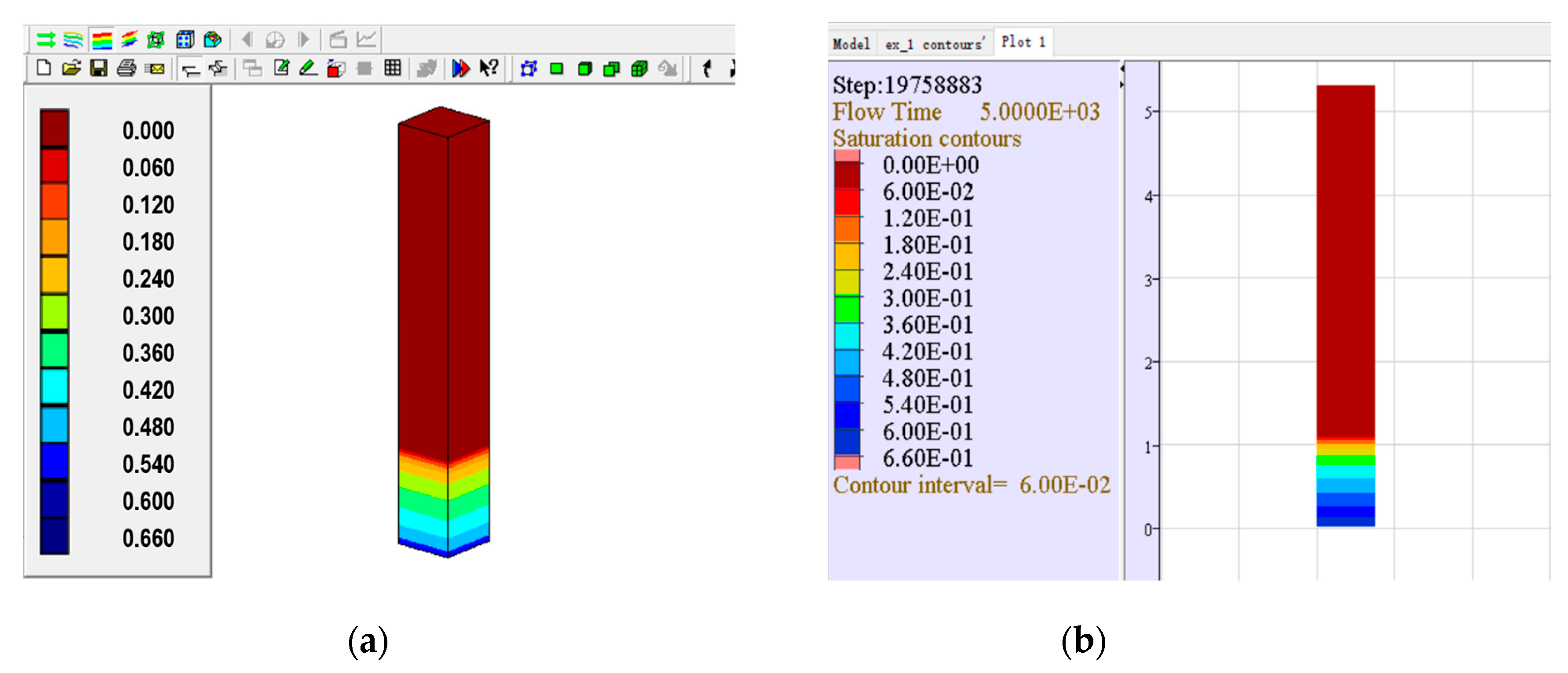
4.1. Water Flooding Oil in the Pillar Rock Sample (LNAPL)

The first example is to simulate a rock sample water displacing oil experiment to test the numerical method presented in this paper. As shown in Figure 4, the static rock sample is filled with oil, such as the initial saturation condition of the water is zero. The initial value of the capillary pressure of the sample for oil and water is measured in advance, for example, the result is water head pressure 25 cm. The side is sealed and the top boundary is kept as a certain fixed pressure. At the beginning of the experiment, water is injected from the bottom boundary with a certain, but slightly higher, pressure to gradually displace most of the oil from the top. The specific pressure values at the top and bottom boundaries are shown in Figure 5.

The capillary pressure head and the relative permeability coefficient depend on water saturation using the formulas of Van Genucheten [28] and Parker et al. [29,30,31]:

$${\mathsf{\psi }}_{\mathrm{c}}={\mathsf{\lambda }}^{-1}{\left({\mathrm{S}}_{\mathrm{we}}^{-1/\mathrm{r}}-1\right)}^{1/\mathrm{n}},$$

(22)

$${\mathrm{k}}_{\mathrm{w}}=\sqrt{{\mathrm{s}}_{\mathrm{we}}}{\left[1-{\left(1-{\mathrm{S}}_{\mathrm{we}}^{-1/\mathrm{r}}\right)}^{\mathrm{r}}\right]}^2,$$

(23)

$${\mathrm{k}}_{\mathrm{o}}=\sqrt{1-{\mathrm{s}}_{\mathrm{we}}}{\left(1-{\mathrm{S}}_{\mathrm{we}}^{-1/\mathrm{r}}\right)}^{2\mathrm{r}},$$

(24)

where, ${\mathrm{S}}_{\mathrm{we}}$ is the effective water saturation, ${\mathrm{S}}_{\mathrm{we}}=\left({\mathrm{S}}_{\mathrm{w}}-{\mathrm{S}}_{\mathrm{wr}}\right)/\left(1-{\mathrm{S}}_{\mathrm{w}}-{\mathrm{S}}_{\mathrm{wr}}\right),{\mathrm{S}}_{\mathrm{wr}}$ and ${\mathrm{S}}_{\mathrm{or}}$ are the residual saturations of water and non-aqueous liquid, respectively; ${\mathrm{k}}_{\mathrm{w}}$ and ${\mathrm{k}}_{\mathrm{o}}$ are the relative permeability coefficients of water and non-aqueous liquid; $\mathsf{\alpha }$ and $\mathrm{n}$ are both van Genuchten constants determined by experimental data; and $\mathrm{r}=1-1/\mathrm{n}$. In this example, $\mathsf{\lambda }=0.431 {\mathrm{cm}}^{-1}$, $\mathrm{n}=3.7$.

The residual saturation of oil, and water are both 0. The required samples and other physical parameters of the liquids are shown in

Table 1. Physical properties of rock sample and fluids (24 °C).

Density/g·${\mathbf{cm}}^{-3}$		Dynamic Viscosity/cp		Sample
Water	Oil	Water	Oil	Porosity	Saturated permeability coefficient/$\mathrm{cm}\cdot {\mathrm{s}}^{-1}$
1.00	0.86	0.914	38.560	0.37	$3.243\times {10}^{-2}$

.

Different from the numerical method above, FLAC2D, version 7.0, is calculating with finite-difference method. Noticed that the sample is a quadrangular, and FLAC considers only a plane model (the third direction is processed by unit length). In order to testify the influence of the sample thickness in this example, a unit thickness was set to the quadrangle and it was found that this is a complete one-dimensional problem. Therefore, the difference in thickness can be ignored. In FLAC, the increments of the nodal pore pressure and saturation are expressed as the following equations [28,32]:

$${\mathsf{\Delta }\mathsf{\psi }}_{\mathrm{w}}=-\frac{\mathsf{\Delta }\mathrm{t}}{\mathsf{\varphi }\mathrm{VD}}\left[{\mathrm{Q}}_{\mathrm{w}}\left(1-\frac{{\mathrm{S}}_{\mathrm{o}}{\mathsf{\psi }}_{\mathrm{c}}^{\prime }}{{\mathrm{K}}_{\mathrm{o}}}\right)+{\mathrm{Q}}_{\mathrm{o}}\right]-\mathsf{\beta }\frac{\mathsf{\Delta }\mathrm{V}}{\mathsf{\varphi }\mathrm{VD}}\left[{\mathrm{S}}_{\mathrm{w}}\left(1-\frac{{\mathrm{S}}_{\mathrm{o}}{\mathsf{\psi }}_{\mathrm{c}}^{\prime }}{{\mathrm{K}}_{\mathrm{o}}}\right)+{\mathrm{S}}_{\mathrm{o}}\right],$$

(25)

$${\mathsf{\Delta }\mathrm{S}}_{\mathrm{w}}=-\frac{\mathsf{\Delta }\mathrm{t}}{\mathsf{\varphi }\mathrm{VD}}\left[{\mathrm{Q}}_{\mathrm{w}}\frac{{\mathrm{S}}_{\mathrm{o}}}{{\mathrm{K}}_{\mathrm{o}}}-{\mathrm{Q}}_{\mathrm{o}}\frac{{\mathrm{S}}_{\mathrm{w}}}{{\mathrm{K}}_{\mathrm{w}}}\right]-\mathsf{\beta }\frac{\mathsf{\Delta }\mathrm{V}}{\mathsf{\varphi }\mathrm{VD}}{\mathrm{S}}_{\mathrm{w}}{\mathrm{S}}_{\mathrm{o}}\left[{\mathrm{S}}_{\mathrm{w}}\left(1-\frac{{\mathrm{S}}_{\mathrm{o}}{\mathsf{\psi }}_{\mathrm{c}}^{\prime }}{{\mathrm{K}}_{\mathrm{o}}}\right)+{\mathrm{S}}_{\mathrm{o}}\right],$$

(26)

$${\mathsf{\Delta }\mathsf{\psi }}_{\mathrm{o}}-{\mathsf{\Delta }\mathsf{\psi }}_{\mathrm{w}}={\mathsf{\psi }}_{\mathrm{c}}^{\prime }{\mathsf{\Delta }\mathrm{S}}_{\mathrm{w}},$$

(27)

$${\mathsf{\Delta }\mathrm{S}}_{\mathrm{w}}+{\mathsf{\Delta }\mathrm{S}}_{\mathrm{o}}=0,$$

(28)

where, by definition:

$$\mathrm{D}=\frac{{\mathrm{S}}_{\mathrm{w}}}{{\mathrm{K}}_{\mathrm{w}}}+\frac{{\mathrm{S}}_{\mathrm{o}}}{{\mathrm{K}}_{\mathrm{o}}}-\frac{{\mathrm{S}}_{\mathrm{w}}}{{\mathrm{K}}_{\mathrm{w}}}\frac{{\mathrm{S}}_{\mathrm{o}}{\mathsf{\psi }}_{\mathrm{c}}^{\prime }}{{\mathrm{K}}_{\mathrm{o}}},$$

(29)

and ${\mathsf{\psi }}_{\mathrm{w}},{\mathsf{\psi }}_{\mathrm{o}},{\mathrm{S}}_{\mathrm{w}},{\mathrm{S}}_{\mathrm{o}}$ are nodal pressure, and saturation of water and non-wetting fluid. ${\mathrm{K}}_{\mathrm{w}},{\mathrm{K}}_{\mathrm{o}}$ are fluid bulk moduli, $\mathrm{V}$ is the nodal volume, $\mathrm{Q}$ is the nodal flow rate, $\mathsf{\beta }$ is the undrained coefficient, which is a constant and equal to one for mechanical coupling and zero for a stand-alone fluid flow calculation. ${\mathsf{\psi }}_{\mathrm{c}}^{\prime }$ is the derivative of the capillary curve.

Differentiating f equations with respect to ${\mathrm{S}}_{\mathrm{w}}$ gives the following Equation (30):

$${\mathrm{S}}_{\mathrm{o}}{\mathsf{\psi }}_{\mathrm{c}}^{\prime }=-{\mathsf{\psi }}_{\mathrm{o}}\frac{1-\mathrm{r}}{\mathrm{r}}\left(1-{\mathrm{S}}_{\mathrm{we}}\right){\mathrm{S}}_{\mathrm{we}}{}^{-1/\mathrm{r}}{\left[1-{\mathrm{S}}_{\mathrm{we}}{}^{1/\mathrm{r}}\right]}^{-\mathrm{r}}$$

(30)

Visualizing the calculated date results from self-development by visualization software, and then generating the saturation distribution contours, the water saturation distribution in the rock sample after 5000 s is shown in Figure 6. The more detailed water distribution information is shown in Figure 7. The water content distribution at that time is shown as Figure 8. The specific water capacity refers to a change in the volumetric water content corresponding to the unit change of pressure head. The distribution of the relative permeability coefficients of water and oil after 5000 s is shown in Figure 9.

As shown in Figure 6, Figure 7, Figure 8 and Figure 9, the results which were calculated by self-developed program are essentially consistent with those correspondingly by FLAC. The discrepancy yet existing between the outcomes from source code and FLAC is due to the difference in numerical formulations between the implicit FEM and explicit finite difference method. Concretely speaking, the latter is an overlaid quadrilateral (four triangular elements for each) ‘element’ as its feature. Additionally, the striking divergence between the theory described before and mentioned in this chapter will also contribute to this subtle difference. It lies in whether the compressibility of fluids is considered.

Therefore, before explaining the specific reason of this discrepancy, it is necessary to clarify the impact of the difference based on the theory first. To simplify the comparison process, a two-dimensional Darcy’s flow was elaborated. In a saturated fluid steady horizontal flow in the ground, if considering the compressibility of the fluid, the governing equations are the follows:

$$-{\left({\mathsf{\rho }\mathrm{u}}_{\mathrm{i}}\right)}_{,\mathrm{i}}=-\frac{\partial }{\partial \mathrm{t}}\left(\mathsf{\rho }\mathsf{\varphi }{\mathrm{S}}_{\mathrm{w}}\right)\mathrm{i}=\mathrm{x},\mathrm{y},$$

(31a)

$$-\frac{\partial }{\partial {\mathrm{x}}_{}}\left({\mathsf{\rho }\mathrm{u}}_{\mathrm{x}}\right)-\frac{\partial }{\partial {\mathrm{y}}_{}}\left({\mathsf{\rho }\mathrm{u}}_{\mathrm{y}}\right)=-\frac{\partial }{\partial \mathrm{t}}\left(\mathsf{\rho }\mathsf{\varphi }·1\right),$$

(31b)

$$-\frac{\partial }{\partial {\mathrm{x}}_{}}\left(\mathsf{\rho }\frac{{\mathrm{k}}_{\mathrm{r}}}{\mathsf{\mu }}{\mathrm{K}}_{\mathrm{xx}}{\frac{\partial \mathsf{\psi }}{\partial {\mathrm{x}}_{}}}_{}\right)-\frac{\partial }{\partial {\mathrm{y}}_{}}\left(\mathsf{\rho }\frac{{\mathrm{k}}_{\mathrm{r}}}{\mathsf{\mu }}{\mathrm{K}}_{\mathrm{yy}}{\frac{\partial \mathsf{\psi }}{\partial {\mathrm{y}}_{}}}_{}\right)=-\frac{\partial }{\partial \mathrm{t}}\left(\mathsf{\rho }\mathsf{\varphi }·1\right),$$

(31c)

$$\frac{{\mathrm{k}}_{\mathrm{r}}}{\mathsf{\mu }}{\mathrm{K}}_{\mathrm{xx}}·{\frac{\partial }{\partial {\mathrm{x}}_{}}}_{}\left(\mathsf{\rho }{\frac{\partial \mathsf{\psi }}{\partial {\mathrm{x}}_{}}}_{}\right)+\frac{{\mathrm{k}}_{\mathrm{r}}}{\mathsf{\mu }}{\mathrm{K}}_{\mathrm{yy}}·{\frac{\partial }{\partial \mathrm{y}}}_{}\left[\mathsf{\rho }·\left(\frac{\partial \mathsf{\psi }}{\partial {\mathrm{y}}_{}}+\mathsf{\rho }\mathrm{gy}\right)\right]=-\frac{\partial }{\partial \mathrm{t}}\left(\mathsf{\rho }\mathsf{\varphi }·1\right),$$

(31d)

$$\frac{{\mathrm{k}}_{\mathrm{r}}}{\mathsf{\mu }}{\mathrm{K}}_{\mathrm{xx}}·{\left(\frac{\partial \mathsf{\rho }}{\partial {\mathrm{x}}_{}}·\frac{\partial \mathsf{\psi }}{\partial {\mathrm{x}}_{}}+\mathsf{\rho }\frac{{\partial }^2\mathsf{\psi }}{\partial {\mathrm{x}}^2{}_{}}\right)}_{}+\frac{{\mathrm{k}}_{\mathrm{r}}}{\mathsf{\mu }}{\mathrm{K}}_{\mathrm{yy}}·{\left[\left(\frac{\partial \mathsf{\psi }}{\partial {\mathrm{y}}_{}}+\mathsf{\rho }\mathrm{gy}\right)\frac{\partial \mathsf{\rho }}{\partial \mathrm{y}}+\mathsf{\rho }\frac{{\partial }^2\mathsf{\psi }}{\partial {\mathrm{y}}^2{}_{}}+\mathrm{gy}·\frac{\partial \mathsf{\rho }}{\partial {\mathrm{y}}_{}}+\mathsf{\rho }\mathrm{g}\right]}_{}=-\frac{\partial }{\partial \mathrm{t}}\left(\mathsf{\rho }\mathsf{\varphi }·1\right),$$

(31e)

while ignoring compressibility of fluid:

$$\frac{{\mathrm{k}}_{\mathrm{r}}}{\mathsf{\mu }}{\mathrm{K}}_{\mathrm{xx}}·{\frac{{\partial }^2\mathsf{\psi }}{\partial {\mathrm{x}}^2{}_{}}}_{}+\frac{{\mathrm{k}}_{\mathrm{r}}}{\mathsf{\mu }}{\mathrm{K}}_{\mathrm{yy}}·{\left(\frac{{\partial }^2\mathsf{\psi }}{\partial {\mathrm{y}}^2{}_{}}+\mathrm{g}\right)}_{}=-\frac{\partial }{\partial \mathrm{t}}\left(\mathsf{\varphi }·1\right),$$

(32)

Comparing Equation (31) with Equation (32), it can be noticed that, in fact, FLAC’s built-in algorithm has considered redundant items $\partial \mathsf{\rho }/\left(\partial \mathrm{x}\right)$ and $\partial \mathsf{\rho }/\partial \mathrm{y}$ (fluid density $\mathsf{\rho }$ can be regarded as the function of moduli ${\mathrm{K}}_{\mathsf{\alpha }}$, while a constant in self-development code), which contributes to the main difference. So as to cut down the deviations to the lowest, the most direct and simple solution is to increase the value ${\mathrm{K}}_{\mathsf{\alpha }}$. However, in realistic calculations, oversized ${\mathrm{K}}_{\mathsf{\alpha }}$ (almost the actual value) will result in a significant increase in the calculation time, as shown in Equation (33), and even terminating the process in order to ensure the convergence for transit seepage flow:

$${\Delta }_{\mathrm{t}}={\mathrm{L}}_{\mathrm{z}}^2\min \left(\frac{1}{{\mathrm{k}}_{\mathrm{w}}{\mathrm{K}}_{\mathrm{w}}},\frac{1}{{\mathrm{k}}_{\mathrm{o}}{\mathrm{K}}_{\mathrm{o}}}\right),$$

(33)

where ${\mathrm{L}}_{\mathrm{z}}$ is the smallest zone size in the simulation, and ${\mathrm{k}}_{\mathrm{o}}$ is the saturated mobility coefficient for the non-wetting fluid (${\mathrm{k}}_{\mathrm{o}}$ = ${\mathrm{k}}_{\mathrm{w}}{\mathsf{\mu }}_{\mathrm{w}}/{\mathsf{\mu }}_{\mathrm{o}}$).

Although it is difficult to precisely position the interface between water and oil, it is believed that the required accuracy can still be attained by finer gridding and longer computational time.

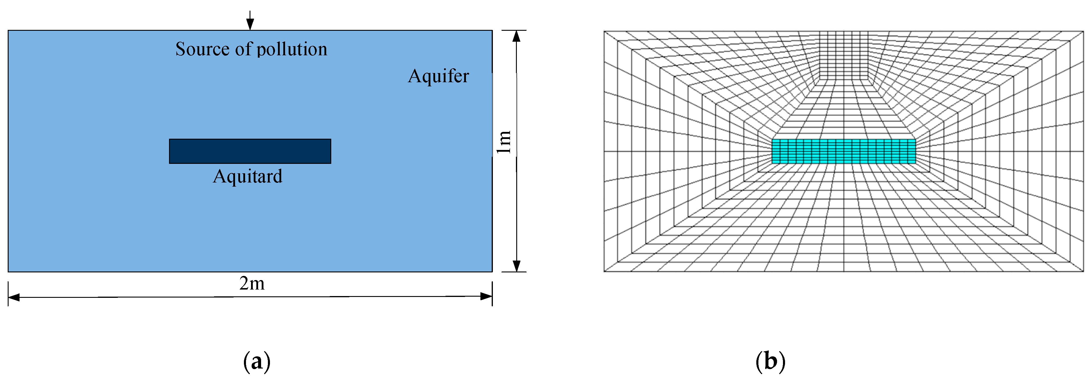
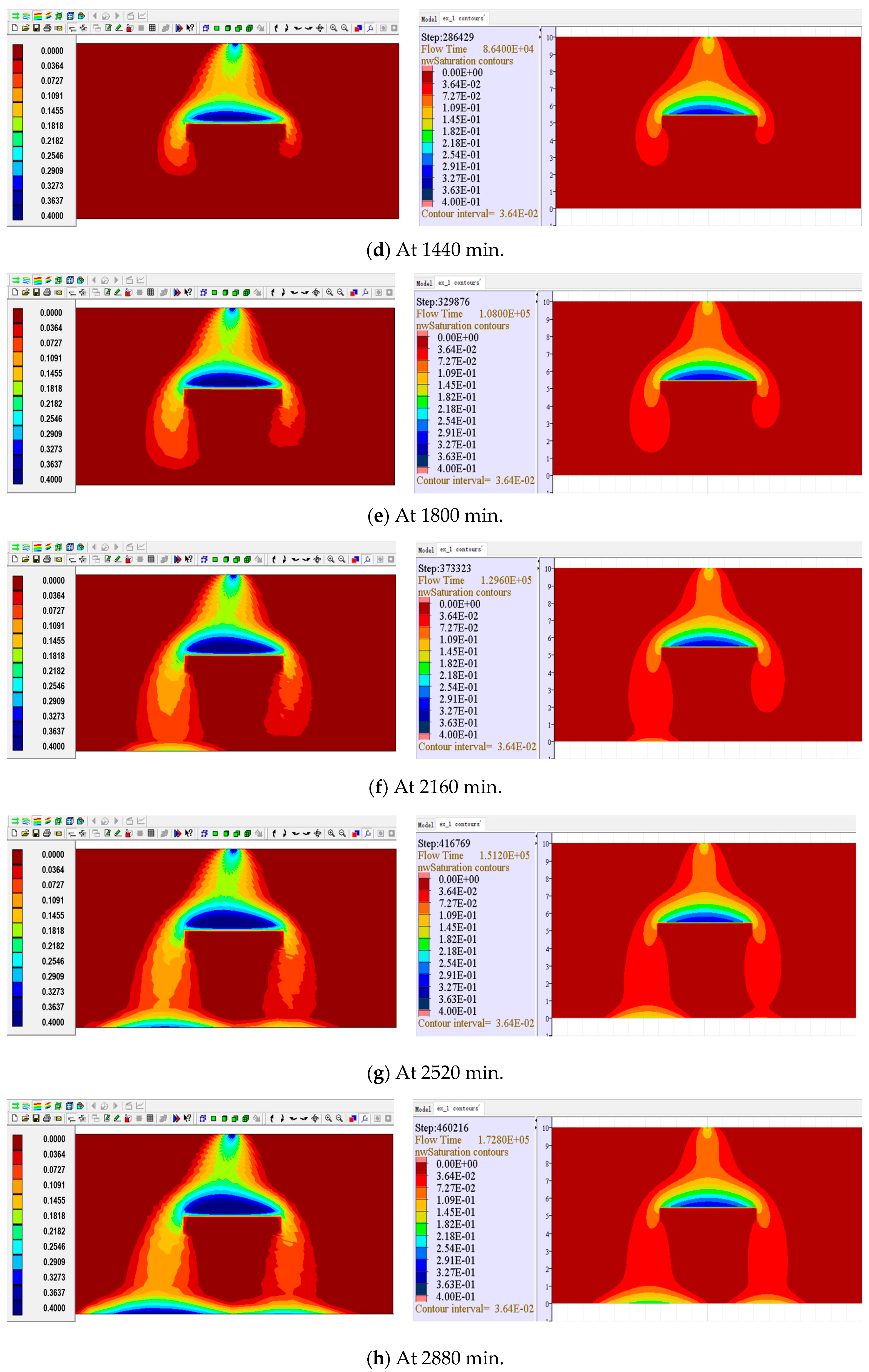
4.2. Simulation of Trichloroethylene Transport in the Aquifer (DNAPL)

The second example is described below. It is used to verify the correctness of the developed program by simulating a typical contamination transport problem. As shown in Figure 10, there is a non-aqueous liquid (trichloroethylene) pressure head with a 0.1 m source at the midpoint of the aquifer model and a low permeability rock formation in the center of the aqueous model (0.667 m × 0.100 m). The top and bottom of the model are impervious borders, while the left and right sides are fixed hydrostatic pressure boundaries based on initial saturation conditions. In the horizontal direction, the water is driven by a 2% pressure gradient and slowly seeps from right to left.

The physical properties of the medium are shown in

Table 2. Physical properties of media (24 °C).

Media	Density $\left(\mathbf{g}·\mathbf{c}{\mathbf{m}}^{-2}\right)$	Dynamic Viscosity $\left(\mathbf{cp}\right)$	Surface Tension $\left(\mathbf{N}·{\mathbf{m}}^{-1}\right)$
Water NAPL Aquifer	999.1 1462.0	0.914 0.55	0.0728 0.0293
Media	Porosity	Hydraulic Conductivity$\left(m·s^{-\mathbf{1}}\right)$	Van Genuchten Parameters
			$r/{\mathrm{m}}^{-\mathbf{1}}$	$n$
Water
NAPL
Aquifer	0.35	$1.0\times {10}^{-5}$	10	2

. For model aquifers and low-permeability aquifers, the residual saturation of water is 5%, while the residual saturation of non-aqueous liquids is 0.5.

The calculation results can be obtained by discretizing the fields and performing numerical simulations using a computer program written in accordance with the finite element formula described above. Meanwhile, the same parameters according to Table 2 in FLAC were set and then this simulation ran. To further verify the correctness of the source program, the numerical simulation result contour figures of the two algorithms after 360 min, 720 min, 1080 min, 1440 min, 1800 min, 2160 min, 2520 min, and 2880 min are compared. As an example, the distribution and variation of trichloroethylene saturation over time in the model domain is shown in Figure 10.

During the infiltration process, under the action of gravity, DNAPL (trichloroethylene) moves in three directions in this model simultaneously and generates an approximately circular pollution area, the closer the place is away from the injection source, the higher the concentration of contaminant. Meanwhile, horizontal flow driving force makes the circular area gradually transform into an elliptical shape, as shown in Figure 11a.

As the infiltration process continues, DNAPL has reached the aquitard and accumulated at the top surface of there, shown in Figure 11b. With the infiltration time increased, DNAPL migration states are shown in the next series of contour figures (Figure 11c–h).

According to these comparison results of the above saturation contours, it can be concluded that either calculated by the self-developed source code or FLAC, the range scale of transport of trichloroethylene in the aquifer after the same time interval is basically regarded as consistent.

These two typical examples have been well simulated using two difference methods: the self-developed finite element method and the advanced finite differential method in FLAC as the existing commercial simulator. The calculation results had both been obtained ideally. They suggest that the comparisons were essentially in consistency, which verifies the correctness of the developed source program, and also show its preliminary practical applicability.

5. Conclusions

In this paper, the procedure of developing three-dimensional finite element method source code programs for the numerical simulation of non-miscible two-phase flows in subsurface water saturated soil is expounded. In the proposed numerical method, the weak forms of mass balance equations for water, NAPLs were discretized in space using the Galerkin finite element method, and mixed-form formulations using both pressure water head and water saturation were adopted. Based on this particular calculation method, two typical examples which belong to LNAPL and DNAPL problems were the modelled cases, respectively. In addition, their outcomes were compared with the results simulated by FLAC. The comparisons demonstrated that they were approximately in coincidental agreement. Therefore, it is convincing that the correctness of the source program is obtained. Moreover, these simulations, having been successfully applied to these problems, also indicates the potential auxiliary analysis potentials of the algorithms developed in this paper on the rock sample displacing experiment and the preliminary evaluation on the migration and diffusion of non-aqueous liquid pollution in the fields. However, it should be noted that the program software developed here is still in its infancy and needs to be further developed and continuously verified based on practical problems in the laboratory and on-site so as to gradually attain consecutive improvements.

References

1. Bernaus, A.; Gaona, X.; Ree, D.V.; Valiente, M. Determination of mercury in polluted soils surrounding a chlor-alkali plant: Direct speciation by X-ray absorption spectroscopy techniques and preliminary geochemical characterisation of the area. Anal. Chim. Acta 2006, 565, 73–80. [Google Scholar] [CrossRef]
2. Bollen, A.; Wenke, A.; Biester, H. Mercury speciation analyses in HgCl2-contaminated soils and groundwater—Implications for risk assessment and remediation strategies. Water Res. 2008, 42, 91–100. [Google Scholar] [CrossRef] [PubMed]
3. Arbestain, M.C.; Rodriguez-Lado, L.; Bao, M.; Macías, F. Assessment of Mercury-Polluted Soils Adjacent to an Old Mercury-Fulminate Production Plant. Appl. Environ. Soil Sci. 2009, 2009. [Google Scholar] [CrossRef]
4. Lynge, E.; Tinnerberg, H.; Rylander, L.; Romundstad, P.; Johansen, K.; Lindbohm, ML.; Heikkilä, P.; Westberg, H.; Clausen, L.B.; Piombino, A.; et al. Exposure to tetrachloroethylene in dry cleaning shops in the Nordic countries. Ann. Occup. Hyg. 2011, 55, 387–396. [Google Scholar] [PubMed]
5. Kvenvolden, K.; Cooper, C. Natural seepage of crude oil into the marine environment. Geo-Mar. Lett. 2003, 23, 140–146. [Google Scholar] [CrossRef]
6. Das, N.; Chandran, P. Microbial degradation of petroleum hydrocarbon contaminants: An overview. Biotechnol. Res. Int. 2011, 1–13. [Google Scholar] [CrossRef] [PubMed]
7. Bear, J. Dynamics of Fluids in Porous Media; Li, J.S., Chen, C.X., Eds.; China Architecture and Building Press: Beijing, China, 1983. (In Chinese) [Google Scholar]
8. Abriolal, M.; Pinder, G.F. A multiphase approach to the modeling of porous media contamination by organic compounds 1. Equation development. Water Resour. Res. 1985, 21, 11–18. [Google Scholar] [CrossRef]
9. Abriolal, M.; Pinder, G.F. A multiphase approach to the modeling of porous media contamination by organic compounds 2. Numerical simulation. Water Resour. Res. 1985, 21, 19–26. [Google Scholar] [CrossRef]
10. Lenhard, R.J.; Oostrom, M.; Dane, J.H. A constitutive model for air-NAPL-water flow in the vadose zone accounting for immobile, non-occluded (residual) NAPL in strongly water-wet porous media (Journal of Contaminant Hydrology (2004) 71 (261-282) doi:10.1016/j.jconhyd.2003.10.014). J. Contam. Hydrol. 2004, 73, 281. [Google Scholar]
11. White, M.D.; Oostrom, M.; Lenhard, R.J. A practical model for mobile, residual, and entrapped NAPL in water-wet porous media. Ground Water 2004, 42, 734–746. [Google Scholar] [CrossRef] [PubMed]
12. Xue, Q.; Liang, B.; Liu, X.L. Study on environmental prediction model of organic contaminants transport in soil-water environment. J. Hydraul. Eng. 2003, 6, 48–55. (In Chinese) [Google Scholar]
13. Wu, D.Y.; Wang, C. Analysis of the Relationship Between the Oil Holdup Measured by Coaxial Conductivity Sensor and the Oil Volume Fraction. J. Tianjin Univ. 2013, 46, 276–280. (In Chinese) [Google Scholar]
14. Chen, J.J.; Yang, J.; Tian, L. Advances in NAPLs transport experiment in porous media based on pore network model. Adv. Earth Sci. 2007, 22, 997–1004. (In Chinese) [Google Scholar]
15. Kleinknecht, S.M.; Class, H.; Braun, J. Density-driven migration of heavy NAPL vapor in the unsaturated zone. Vadose Zone J. 2015, 14. [Google Scholar] [CrossRef]
16. Kikumoto, M.; Nakamura, K. Simulation of seepage flow of non-aqueous phase liquid in vadose zone. Environ. Geotech. 2017, 4, 171–183. [Google Scholar] [CrossRef]
17. Javanbakht, G.; Arshadi, M.; Qin, T.; Goual, L. Micro-scale Displacement of NAPL by Surfactant and Microemulsion in Heterogeneous Porous Media. Adv. Water Resour. 2017, 105, 173–187. [Google Scholar] [CrossRef]
18. Joun, W.; Lee, S.-S.; Koh, Y.E.; Lee, K.-K. Impact of water table fluctuations on the concentration of borehole gas from NAPL sources in the vadose zone. Vadose Zone J. 2016, 15. [Google Scholar] [CrossRef]
19. Xie, B.; Kong, D.; Kong, L.; Kong, W.; Li, L. Analysis of vertical upward oil-gas-water three-phase flow based on multi-scale time irreversibility. Flow Meas. Instrum. 2018, 62, 9–18. [Google Scholar] [CrossRef]
20. Tan, C.; Li, P.; Dai, W.; Dong, F. Characterization of oil-water two-phase pipe flow with a combined conductivity/capacitance sensor and wavelet analysis. Chem. Eng. Sci. 2015, 134, 153–168. [Google Scholar] [CrossRef]
21. Picchi, D.; Battiato, I. The Impact of Pore-Scale Flow Regimes on Upscaling of Immiscible Two-Phase Flow in Porous Media. Water Resour. Res. 2018, 54, 6683–6707. [Google Scholar] [CrossRef]
22. Balasuriya, S. Transport between two fluids across their mutual flow interface: The Streakline Approach. SIAM J. Appl. Dyn. Syst. 2017, 16, 1015–1044. [Google Scholar] [CrossRef]
23. Li, Y.; Gao, J.; Liu, X.; Xie, R. Energy demodulation algorithm for flow velocity measurement of oil-gas-water three-phase flow. Math. Probl. Eng. 2014, 5, 1–13. [Google Scholar] [CrossRef]
24. Kacem, M.; Benadda, B. Mathematical Model for Multiphase Extraction Simulation. J. Environ. Eng. USA 2018, 144. [Google Scholar] [CrossRef]
25. Bear, J.; Cheng, H.D. Modeling Groundwater Flow and Contaminant Transport; Springer: Berlin, Germany, 2010. [Google Scholar]
26. Bear, J. Dynamics of Fluids in Porous Media; American Elsevier: Amsterdam, The Netherlands, 1972; Volume 764. [Google Scholar]
27. Celia, M.A.; Bouloutas, E.T.; Zarba, R.L. A general mass-conservative numerical solution for the unsaturated flow equation. Water Resour. Res. 1990, 26, 1483–1496. [Google Scholar] [CrossRef]
28. Van Genucheten, M.T. A closed-form equation for predicting the hydraulic conductivity of unsaturated soils. Soil Sci. Soc. Am. J. 1980, 44, 892–898. [Google Scholar] [CrossRef]
29. Parker, J.C.; Lenhard, R.J.; Kuppusamy, T. A parametric model for constitutive properties governing multiphase flow in porous media. Water Resour. Res. 1987, 23, 618–624. [Google Scholar] [CrossRef]
30. Parker, J.C.; Lenhard, R.J. A model for hysteretic constitutive relations governing multiphase flow: 1. Saturation–pressure relations. Water Resour. Res. 1987, 23, 2187–2196. [Google Scholar] [CrossRef]
31. Parker, J.C.; Lenhard, R.J. A model for hysteretic constitutive relations governing multiphase flow: 2. Permeability–saturation relations. Water Resour. Res. 1987, 23, 2197–2206. [Google Scholar] [CrossRef]
32. Nikolaevskii, V.N. Mechanics of Porous and Fractured Media; World Scientific: Singapore, 1990. [Google Scholar]
Figure 1. Schematic illustration of the subsurface transport mechanism of NAPL contaminants.
Processes 07 00116 g001
Figure 2. Mass conservation of flows passing through a small rectangular parallelepiped.
Processes 07 00116 g002
Figure 3. Nonlinear character of water and NAPL two-phase flow: (a) Two-phase flow characteristic curve of the water-non-aqueous liquid; and (b) the relative permeability coefficient of each phase depends on the change of the water phase saturation.
Processes 07 00116 g003
Figure 4. Illustration of inability of using single form formulation to model immiscible flow.
Processes 07 00116 g004
Figure 5. Displacing test thorough a rock sample: (a) Model size and boundary conditions; and (b) model meshing.
Processes 07 00116 g005
Figure 6. Contrast of simulated water saturation distribution after 5000s: (a) Instantaneous water saturation distribution calculated by self-developed source codes; and (b) instantaneous water saturation distribution calculated by FLAC.
Processes 07 00116 g006
Figure 7. Simulated water-phase saturation distribution after 5000 s.
Processes 07 00116 g007
Figure 8. Simulated specific volumetric water content distribution after 5000 s.
Processes 07 00116 g008
Figure 9. Simulated relative permeability distribution after 5000 s.
Processes 07 00116 g009
Figure 10. Aqueous model test: (a) Model size and boundary conditions; and (b) model meshing.
Processes 07 00116 g010
Figure 11. Distribution of saturation with regards to trichloroethylene and its change with time simulated using self-developed source code (left) and FLAC (right).
Processes 07 00116 g011aProcesses 07 00116 g011b