Ion Exchange Dialysis for Aluminium Transport through a Face-Centred Central Composite Design Approach

Abstract

An ion exchange dialysis (IED) is used in the recovery of aluminium from residue. In this paper, the face-centred central composite design (FC-CCD) of the response surface methodology (RSM) and desirability approach is used for experimental design, modelling and process optimization of a counter flow IED system. The feed concentration, feed flowrate, sweep flowrate and sweep concentration were selected as the process variables, with the Al transport across a Nafion 117 membrane as the target response. A total of 30 experimental runs were conducted with six centre points. The response obtained was analysed by analysis of variance (ANOVA) and fitted to a second-order polynomial model using multiple regression analysis. The actual R² and standard deviation of the model are 0.9548 and 0.2932, respectively. Depending on the time zone of reference (24 h or 32 h), the highest enrichment of >1.50 was achieved. The designed variables were numerically optimized by applying the desirability function to achieve the maximum Al transport. The optimised condition values were found to be a feed concentration of 1600 ppm, feed flowrate of 61.76%, sweep flowrate of 37.50% and sweep concentration of 0.75 N for the 80% target response at 32 h. Overall, the model can be used to effectively predict Al recovery using the designed system.

1. Introduction

Water is essential to life and the proper functioning of ecosystems on earth. Due to the global economic drive associated with population growth, water withdrawal pressures from households, industries and agriculture is expected to escalate. The challenge of meeting and efficiently distributing water to address the competing demand from various sectors can therefore not be associated to availability only, rather, availability and quality of the water. The major task of water treatment plants (WTPs) are therefore to meet allowable limits on standards set for water quality parameters.

Coagulation is an important step used in urban water treatment schemes to achieve water quality standards. This conventionally known technology is relatively easy to design, simple to operate and has low energy utilization [1]. The process requires dosing coagulants to coalesce impurities into large masses for subsequent removal by other treatment processes. Common coagulants such as aluminium sulphate, aluminium chloride, poly aluminium chloride, sodium aluminate, ferric chloride and ferric sulphate are used to achieve this physicochemical process in water treatment [2,3]. Aluminium sulphate has been the most widely used coagulant by WTPs. It is known to generate a large amount of water treatment residue. As such, the recovery and utilization of the residue can serve as a secondary source of the coagulant. However, large-scale implementation of coagulant recovery by acidification and reuse of the leachate in the 1970s was withdrawn [4]. Similar to alkaline leaching, the process lacked specificity and selectivity. While recovery by pressure driven membrane techniques on water treatment residue is faced with fouling issues and high energy demand, the main obstacles of ion exchange resins are fouling by organic compounds and resin regeneration [5,6].

Ion exchange membranes (IEMs) are used in water/wastewater treatment, food manufacturing/processing, chemical synthesis and energy harvest and storage [7,8,9,10]. These plastic films are classified into cation exchange membranes (CEMs) and anion exchange membranes (AEMs). The CEMs are embedded with fixed negative charges, and thus permeates ions of opposite charge (counter ions) and excludes ions of the same charge (co-ions). In turn, AEMs have fixed positive charge groups. Their functionality is a combination of membrane permeability and electrochemical properties of ion exchange resins [8]. The CEMs and AEMs are composed of hydrophilic ionic groups and anchored by hydrophobic polymer chains. Notable amongst the hydrophilic functional moieties in CEMs are SO₃⁻, PO₃H⁻, –COO⁻, PO₃²⁻ and C₆H₄O⁻, and that of AEMs are NH₃⁺, NRH²⁺, NR₂H⁺, NR₃⁺ and PR₃⁺ [11,12,13].

Ion exchange dialysis (IED), popularly known as Donnan dialysis (DD), employs IEMs for selective transport, removal and separation of ions of interest. The technology is an electrochemical potentially driven process that separates and concentrates ions from aqueous solutions by the stoichiometric counter transport of ions across the IEM. Ions of interest diffuse from the donor or feed phase to the acceptor or sweep phase. An exchanging electrolyte in the acceptor phase with a higher concentration of the same charge as the ion of interest permeates into the donor phase. The fundamental principle of Fredrick G. Donnan’s 1924 study established the Donnan equilibrium from the electrostatic repulsion of co-ions from the phases [14]. Electrolytic solutions are at equilibrium when the electrochemical potential difference across the membrane equates to the Donnan potential of the membrane [15]. Theoretically, IED or the DD process is not prone to fouling [16] and has a low energy consumption. Another functional primacy of the simple and cost effective IED system is their insignificant electrochemical altering of analyte and enrichment of analyte [17]. These characteristics make it a potentially useful green treatment technology for removal, separation, purification and concentration of ions of interest.

Different commercial IEMs have been used in IED studies, including CEMs such as Pall ICE-450 (SA3S and SA3T), Neosepta (CMS, CMX), Selemion (CMV), Ultrex CMI 7000 and Nafion (417 and115) [18,19,20,21,22,23]. Notable AEMs such as Neosepta (ACS, AMX, AFN and AEX), Ionics (AR204-UZRA and AR103-QPD), Polymerchemie-PC (SA, 100D, acid 60 and acid 100), Fumasep (FTAM and FAB), Jam-1 and Selemion (AMV) have been reported [24,25,26,27,28,29,30,31]. The Nafion 117 CEM has been used in the kinetic studies of monovalent (such as K⁺, Na⁺ and Cs⁺) and divalent (Ca²⁺ and Mg²⁺) transport [32,33,34,35]. Further records on the application of IED using Nafion 117 for Al³⁺ have shown a high recovery of >70% [16]. Despite the high Al recovery, there is limited information on the effect of process variables on Al transport through Nafion 117 CEMs. A comparative study on the effect of sweep concentration and different membranes (homogeneous Nafion 117 and heterogeneous Ionac 3470) on the recovery was performed using a one-factor-at-a-time (OFAT) approach [36].

As the standardization of process variables is essential for effective Al transport, the limitation incorporated with the classical OFAT technique is its incapability in optimizing the overall process in a short time with a low number of experimental runs for a multivariate system. These inadequacies can be eliminated via a computed statistical standardization viz. the response surface methodology (RSM). The response surface methodology is a systematic methodology that consists of a group of mathematical and statistical techniques for experimental design, independent and interdependent analysis, model development and exploitation [37,38]. The empirical model (Equation (1)) is a relationship between process variables and the expected response to understand the process mechanism and to optimize the process using minimal experimental runs [39]. Important areas of RSM application are product design, development and formulation, and improvement of existing products [40].

$$y={\beta }_o+{\displaystyle {{\displaystyle \sum }}_{n=1}^n}{\beta }_i{x}_i+{\displaystyle {{\displaystyle \sum }}_{i=1}^n}{\beta }_{ii}{X}_i^2+{\displaystyle {{\displaystyle \sum }}_i^{i<j,k}}{{\displaystyle \sum }}_{j,k}{\beta }_{ijk}{x}_i{x}_j{x}_k+\epsilon ,$$

(1)

where y is the transmittance function; $\beta$_o is a constant coefficient; $\beta$_i is a linear coefficient; $\beta$_ii is the quadratic coefficient; $\beta$_ijk is the interaction coefficient; $\epsilon$ is the random error; and k is the number of variables studied.

With an industrial concept mind, Asante-Sackey et al. [41] designed a counter-flow IED system to study aluminium permeation across a Nafion 117 membrane using a statistical order. In this present work, the multivariable interactive effect of feed concentration, feed flowrate, sweep concentration and sweep flowrate on Al permeation using the face-centred central composite design (FC-CCD) approach is reported. The option of the FC-CCD was to operate the process in the extreme region at the corners of the square at three levels for each variable setting. Hence, investigation of the aforementioned parameters within the RSM context allows the evaluation of the statistical significance of the variables by a mathematical model equation via the F-test for analysis of variance (ANOVA). Furthermore, the mobility of Al and the synergic effect of the process variables with respect to the two different time intervals was compared statistically. This provided a basis for the prediction of the effects of the significant process variables on Al transport at different time zones. The ability of the Nafion 117 to concentrate aluminium was also examined for the feed and sweep volume ratio used for the study and at the different sweep concentrations used. Lastly, the experimental evaluation of the optimum conditions for maximum recovery was performed and reported using the desirability approach. Most previous research on IED or DD have not used the RSM approach and this sets a precedence generally in this field and specifically in Al recovery.

2. Materials and Methods

2.1. Materials and Chemicals

Al₂(SO₄)₃·18H₂O (≥97%) and HCl (32% w/w) was supplied by Lichro Chemicals, South Africa. Demineralized water (17.5 MΩ/cm, Purite-HP+BOOST 030773) was used. These reagents were used without further purification. The Nafion 117 with an equivalent weight of 1100 g, thickness of 177.8 µm and ion exchange capacity of 0.94 meq/g (as provided by the manufacturers) was used for this experiment. Generally, Nafion (C₇HF₁₃O₅S·C₂F₄) is a long side chain thermoplastic resin made by the copolymerization of hydrophobic tetrafluorothylene and perfluorovinyl ether which is terminated at the end with a sulfonyl fluoride (SO₂F). Preceding acid treatment (3 wt% HCl, 90 °C, 1 h), the CEM was soaked in demineralized water for 15 min, heated at 60 °C in 3 wt% H₂O₂, and rinsed with demineralized water. Further treatment steps included pre and post rinsing with demineralized water after another acid conditioning (1 wt% HCl, 25 °C, 180 min) for 15 min.

2.2. Experimental Design and Statistical Analysis

The most commonly used RSM for three to a maximum of six factors is the central composite design (CCD). This design was originally developed by Box–Wilson. The CCD uses an incomplete full factorial or fractional factorial to develop the second order polynomial model. For efficient evaluation of first and second order terms and the estimation of curvatures, the CCD arguments the full or factorial design with axial points and replication of centre points. The axial points are symmetrical with the centre points on the coordinate system at a distance “α” from the design centre. The CCD is made up of the face-centred (FC), central composite circumscribed (CCC) and central composite inscribed (CCI). The CCC has axial points that are the same distance “α” from the centre points, and the “α” values are used to establish the extremes for the low and high limits of each variable. On the other hand, CCI is a scaled down CCF, with the limits for each variable as the main limits, and using the limits as the axial points and creating a factorial or fractional factorial design within the limits. However, in the FC, the “α” value is ±1, such that the axial points are at the centre of each face of the factorial space [42,43].

Design Expert version 11.1.2 software (State-Ease Inc., Minneapolis, MN, USA) was used for the design, evaluation, mathematical modelling and optimization (Figure 1). The independent variables used in this study were feed concentration (Al; X₁), feed flowrate (%; X₂), sweep flowrate (%; X₃) and sweep concentration (HCl; X₄). The Al³⁺ transport (Y₁) was considered as the dependent factor (response). Performance of the counter flow IED system was evaluated by analysing the Al in the feed and sweep chambers.

The four independent variables were converted into a dimensionless form. Three different normalized levels of each variable were designated according to the FC-CCD coding as −1, 0 and 1, respectively. Conversion of the selected independent variables into dimensionless codified values is to ensure comparison of factors of different natures with different units and to decrease the error in the polynomial fit according to Equation (2) for the statistical analysis.

$$x_i=\frac{X_i-X_0}{\Delta X}i=1,2,\dots ,k,$$

(2)

where x_i is the dimensionless coded value of the i-th independent variable; X_i is the un-coded value of the i-th independent variable; X_i is the real value of the independent variable; X₀ is the value of X_i at the centre point; and $\Delta$X is the step change value of the variable i.

The system’s behaviour is defined by the empirical second-order polynomial model [44].

Table 1. Coded and actual values of variables of the design of experiments for overall Al-transport optimization.

Symbol	Variable	Coded Levels of Variables
		−1	0	1
X1	Feed concentration (ppm)	100	1050	2000
X2	Feed flowrate (%)	25	55	85
X3	Sweep flowrate (%)	25	55	85
X4	Sweep concentration (N)	0.25	0.625	1

shows the independent variables and their respective levels for the FC-CCD used in the present study. The design consists of a first order 2^k factorial portion augmented by 2k axial points and accentor runs (cp), where k is the number of variables. Information about the response system and evaluation of the significance of the factors is mostly achieved at the first order design [42]. According to the FC-CCD matrix, Table 1, a total of 30 (=2^k + 2k + cp) runs comprising of 16 factorial points, 8 axial points and 6 centre points is required. The remaining five are centre point replications to get a good estimation of the experimental error via the sum of squares. Furthermore, the proposed matrix by the software was randomized in order to prevent systematic error.

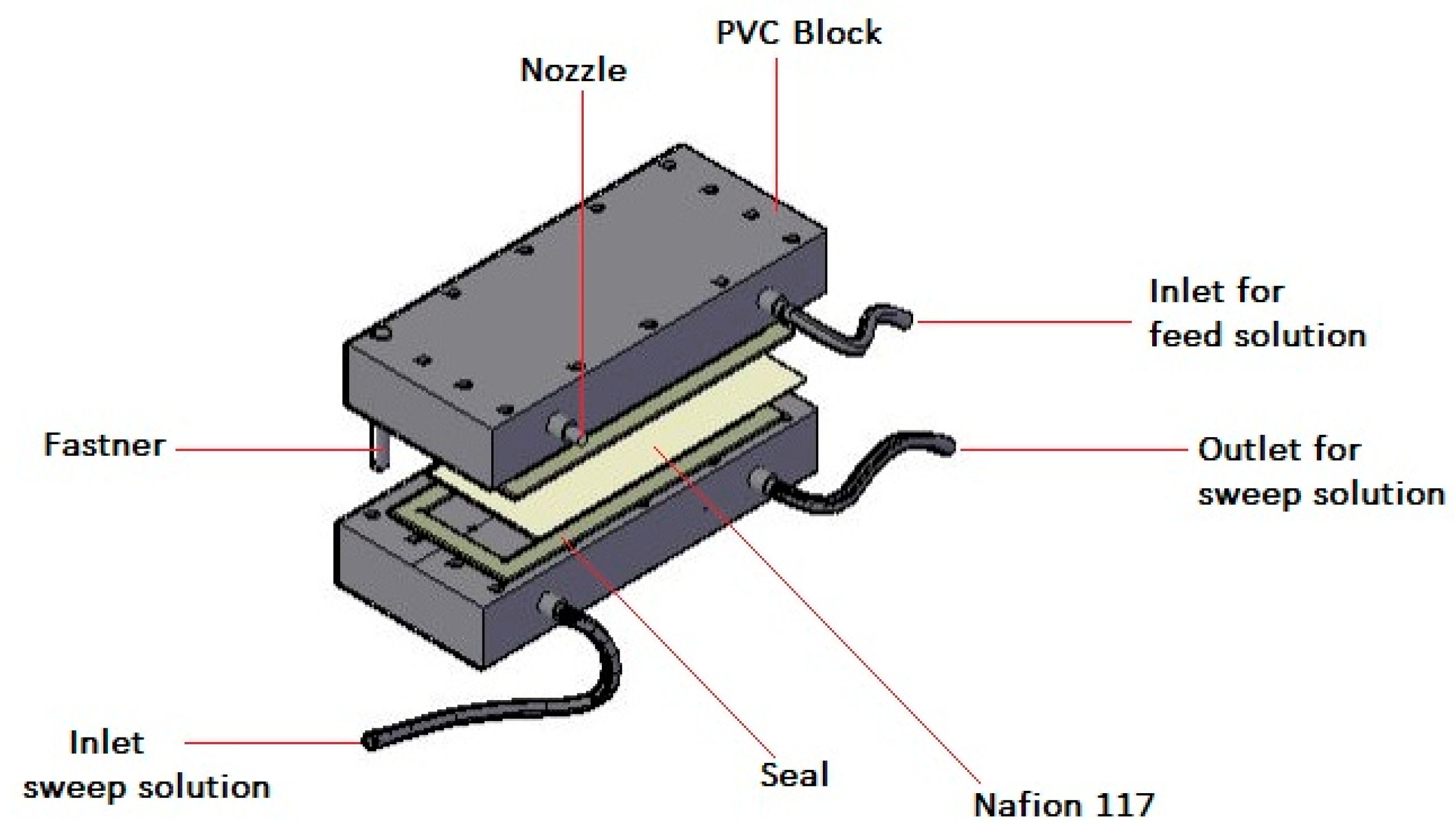
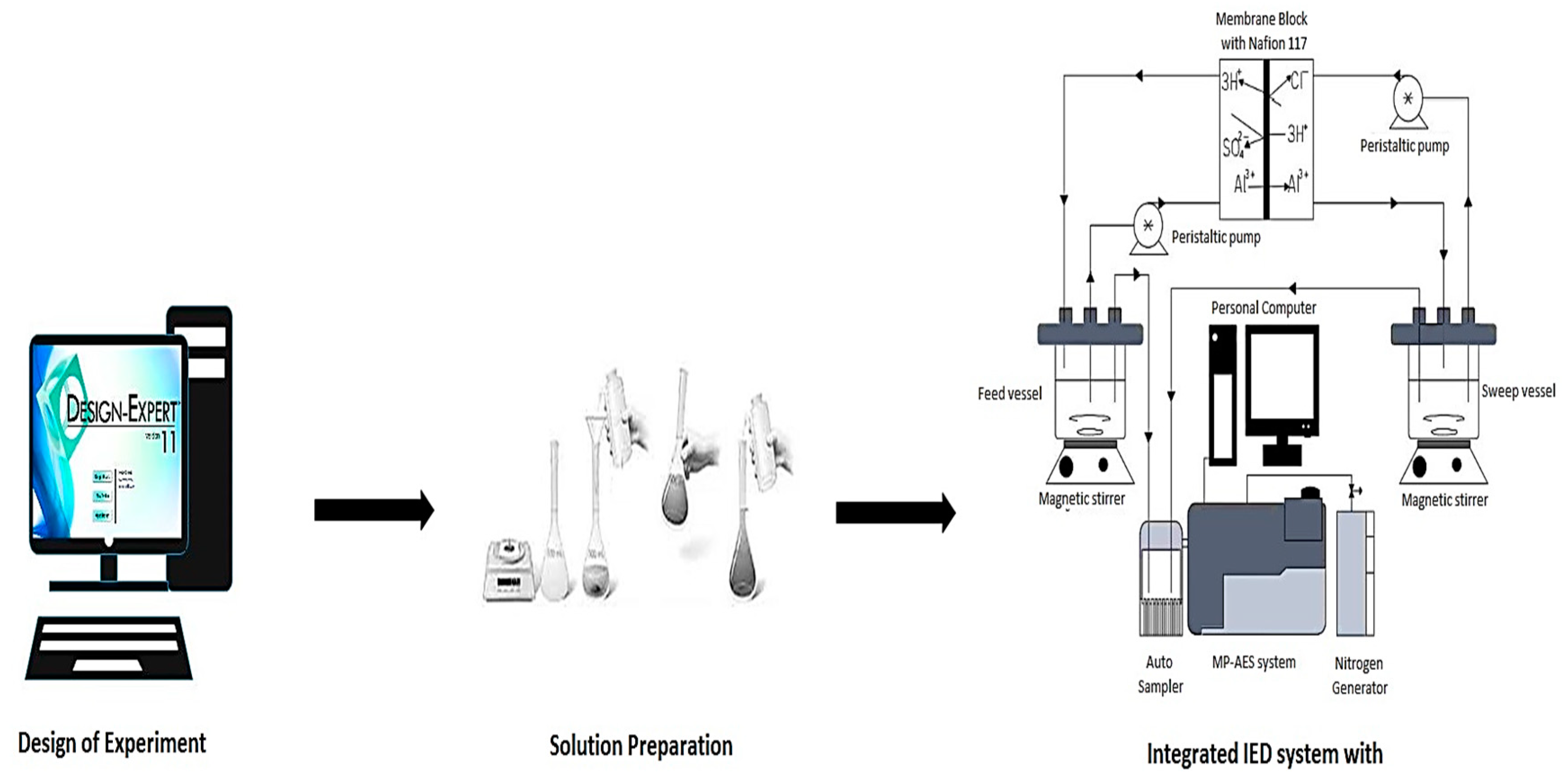
2.3. Ion Exchange Dialysis Set-Up

The IED process was conducted using a laboratory flat sheet dialytic set-up equipped with the CEM (Figure 1) with a working area of 205 cm². The process involved recirculation of the feed and sweep with a pump of maximum flowrate of 2.6 mLs⁻¹. Pump calibration was performed using a randomized complete block design in order to reduce residual error and controlling nuisance factors. The volume ratio of the feed to the sweep was 2:1. The feed and sweep electrolyte solutions were prepared as provided in Table 1 and homogeneity was ensured during the experiment with the aid of magnetic stirrers. Previous work done by the authors expounds on the choice of the ranges for the variables of concern [41]. All experiments were performed in an air-thermostated room between 22 and 25 °C. The data obtained was evaluated in terms of Al transport (%) from the feed solution as follows:

$$Y\left(transport\right)\left(Al\right)=\frac{{\left[Al\right]}_{feed\left(0\right)-}{\left[Al\right]}_{feed\left(t\right)}}{{\left[Al\right]}_{feed\left(0\right)}}\times 100\%$$

(3)

where [Al]_feed(0) and [Al]_feed(t) denote, respectively, the aluminium concentrations at time t = 0 and at an elapsed time, t, in the feed compartment.

Common sources of leaks that could hinder experiment integrity, such as tears in the tubes, membranes and inner tubing of the peristaltic pumps, were checked. Peristaltic pump tubing was replaced periodically to check inner wearing that could be due to the concentration of solutions used. A schematic flow of the experimental setup for Al transport is shown in Figure 2.

2.4. Analytical

The Al transport from the feed phase to the sweep phase was measured using the Agilent micro-plasma atomic emission spectrophotometer (MP-AES, MY 18379001). Samples collected from the two phases were diluted (5–100 times) with 1 wt% HNO₃ to volume. The total loss of the feed and sweep solution due to sampling was between 3% and 4% of the total volume [41].

3. Results

The results from the experimental design matrix is presented in

Table 2. Experimental design matrix and observed responses at different time zones.

Run Order	Variable Level				Response (%)
	X1	X2	X3	X4	24 h	32 h
1	1	−1	−1	−1	28.55	35.95
2	1	1	1	−1	33.35	45.65
3	−1	1	−1	−1	75.90	84.10
4	1	−1	1	1	61.6	71.85
5	−1	−1	−1	1	70.2	78.25
6	0	0	0	0	79.1	86.00
7	1	1	−1	1	64.25	73.45
8	−1	−1	1	−1	58.15	61.60
9	−1	1	1	1	86.95	93.55
10	0	0	0	0	78.82	86.05
11	−1	1	−1	1	87.50	94.85
12	0	0	0	0	78.36	85.96
13	0	0	0	0	78.62	85.85
14	1	1	1	1	51.60	63.85
15	−1	1	1	−1	81.40	90.00
16	−1	−1	1	1	57.95	68.75
17	1	1	−1	−1	32.55	32.85
18	1	−1	−1	1	56.95	66.95
19	−1	−1	−1	−1	58.80	65.85
20	1	−1	1	−1	30.25	34.50
21	0	0	0	0	78.98	86.01
22	0	−1	0	0	52.57	60.52
23	−1	0	0	0	78.55	84.98
24	0	0	0	1	84.81	90.19
25	0	1	0	0	72.19	80.71
26	0	0	1	0	66.95	77.33
27	0	0	0	0	78.99	87.12
28	0	0	−1	0	75.90	81.90
29	0	0	0	−1	48.71	54.48
30	1	0	0	0	50.65	58.75

in a randomized order. The Al recovery at different time intervals showed the effect on each variable at their different interactional levels. Statistical analysis of the response is performed using the various responses obtained.

4. Discussion

4.1. Regression Models and Statistical Testing

Statistical analysis of the present Al mobility was performed with analysis of variance (ANOVA). In ANOVA, a comparison was performed for variation due to change in the levels of variables with variations associated to random errors inherent in the measurement of the response (Al transport). The proportion of influence of a set of variables was therefore assessed towards adequacy and validation of the regression model according to the Fisher test (F-test) and the probability value (p-value at 95% confidence level). As such, the highest order polynomial with significant terms that showed the correlation between variables well and normally (not aliased) would be selected. As shown in

Table 3. Sequential model sum of squares for model generation at 32 h.

Source	Sum of Squares	Df	Mean Square	F-Value	p-Value (Prob > F)
Mean vs. Total	2130.42	1	2130.42
Linear vs. Block	24.49	4	6.12	12.09	<0.0001
2FI vs. Linear	4.74	6	0.7899	1.94	0.1316
Quadratic vs. 2FI	5.79	4	1.45	16.72	<0.0001
Cubic vs. Quadratic	0.7625	8	0.0953	1.32	0.3974
Residual	0.3623	5	0.0725
Total	2166.56	28

, a high F-value was found with the quadratic vs. two factor interaction (2FI) followed by the linear vs. block source. While there was an observed distortion for the cubic vs. quadratic model, their F-value and that of 2FI vs. linear was insignificant. The model selection was therefore found between quadratic and 2FI. Subsequently, the model selected was based on the low standard deviation (SD) and the high value of the actual regression coefficient (act-R²) [45].

As shown in

Table 4. Statistical analysis of the models at 32 h.

Response	Source	Standard Deviation	Actual R2	Adjusted R2	Predicted R2
Al3+ transport	Linear	0.7117	0.6776	0.6216	0.4387
	2FI	0.6376	0.8088	0.6963	0.3961
	Quadratic	0.2941	0.9689	0.9354	0.8034
	Cubic	0.2692	0.9900	0.9459	−3.6866

, despite the lower standard deviation and high act-R² recorded for the cubic model (0.27 and 0.99, respectively), the quadratic model showed a better correlation than the cubic, linear and 2FI models. The efficiency of variability in the actual response values can be expounded on by the experimental value and their interactions as given by the act-R². However, the acceptable difference between the act-R² and the adj-R² should be less than 0.2 [40]. Statistically, a high adj-R² (>0.75) is acceptable [46].

The selected model in terms of the coded and actual values are provided in Equations (4) and (5), respectively. The coded equation (Equation (4)) can be used to make a response prediction for the given coded levels (Table 1) of each process variable. By comparing the coefficients of the terms, the coded equation becomes useful for identifying the relative impact of the terms. The synergetic effect of the model terms are represented by their positive signs (X₂, X₄ and X₁X₄) while the negative signs (X₁, X₁X₂$, X_1^2, X_2^2$ and $X_4^2$) indicates the antagonistic effect. The actual values of the model terms in their specified units can be fitted into Equation (5) to predict the Al³⁺ transport at 32 h.

Coded equation:

$$\sqrt{Y_{Al}}=+9.20-0.8414\left(X_1\right)+0.3718\left(X_2\right)+0.7170\left(X_4\right)-0.2779\left(X_1{X}_2\right)+0.4334\left(X_1{X}_4\right)-0.4093\left(X_1^2\right)-0.4693\left(X_2^2\right)-0.4120\left(X_4^2\right).$$

(4)

In terms of actual values, the model terms are given by

$$\begin{array}{ll}Al(\%)& =5.26811-(0.000157*feedconc.)\\ & +(0.079990*feedflow)\\ & +(4.29677*Sweepconc.)\\ & -(9.75258E-06*feedconc.*feedflow)\\ & +(0.001217*feedconc.*sweepconc.)\\ & -(4.53502E-07*feedconc{.}^2)-(0.000521*feedflo{w}^2)\\ & -(2.92973*sweepconc{.}^2).\end{array}$$

(5)

Unlike the synergetic effect of feed concentration in the simplified model developed in the previous work at 24 h [41], the feed concentration in the actual model for 32 h contributed antagonistically to the Al recovery. Furthermore, while the quadratic term of sweep concentration was significant at 32 h, vice versa was observed at 24 h.

4.1.1. Analysis of Variance (ANOVA)

The independent variables in the selected model and the impact of each variable were then evaluated. For this purpose, the adequacy of the quadratic model was evaluated using several assessments, such as the coefficient of determination, adjusted coefficient and the coefficient of variation (CV). The value of the act-R² indicates the percentage of the variation in the response that is attributed to the input variables [47]. In

Table 5. ANOVA for reduced quadratic model at 32 h.

Source	Sum of Squares	Df	Mean Squares	F-Value	p-Value Prob > F
Regression model	34.51	8	4.31	50.18	<0.0001
X1-Feed conc.	12.74	1	12.74	148.28	<0.0001
X2-Feed flow	2.49	1	2.49	28.95	<0.0001
X4-Sweep conc.	9.25	1	9.25	107.66	<0.0001
X1X2	1.24	1	1.24	14.38	0.0012
X1X4	3.01	1	3.01	34.97	<0.0001
$X_1^2$	0.4585	1	0.4585	5.33	0.0323
$X_2^2$	0.6027	1	0.6027	7.01	0.0159
$X_4^2$	0.4645	1	0.4645	5.40	0.0313
Residuals	1.63	19	0.0859
Pure Error	0.0018	3	0.0006

Standard deviation = 0.2932; Mean = 8.43; CV % = 3.48; Actual R² = 0.9548; Predicted R² = 0.8736; Adjusted R² = 0.9358; Adequate Precision = 22.8386.

, the indicated act-R² of 0.9548 was close to 1. This represented 95.48% variability of the predicted response value (Al³⁺ transport), which is a function of the four process variables. The adj-R² (0.9358) also represents 0.0642 of the variations in the response that cannot be attributed to the significant independent terms. The clear exemption of statistically insignificant terms in the model was through the forward screening method under the condition (p-value ≤ α = 0.05).

The ANOVA in Table 5 revealed that the first order (X₁, X₂, X₄), two way interaction (X₁X₂ and X₁X₄) and pure quadratic effect ($X_1^2,X_2^2$ and $X_4^2$) were highly significant for Al³⁺ transport. More so, the F-value of 50.18 implied the model term was statistically significant and there was only a 0.01% chance that the large F-value could be due to noise. F-values of the independent variables X₁, X₂ and X₃ were 148.28, 28.95 and 107.66, respectively. Considering the F-values, the effect of the independent variables on Al³⁺ mobility was therefore high for variables with a high F-value. The calculated CV of 3.48% further assented to the reliability of the model. A measure of the relative dispersion with respect to the mean provides information on the reproducibility, repeatability and precision of the model, where CV < 10% [48,49]. The adequate relationship between the signal–to-noise ratio must also exist to inform that the model can be used to navigate the design space. The signal-to-noise ratio, given by the adequacy precision, was 22.839, which is >4. Therefore, the noise level did not compete with useful information from the model.

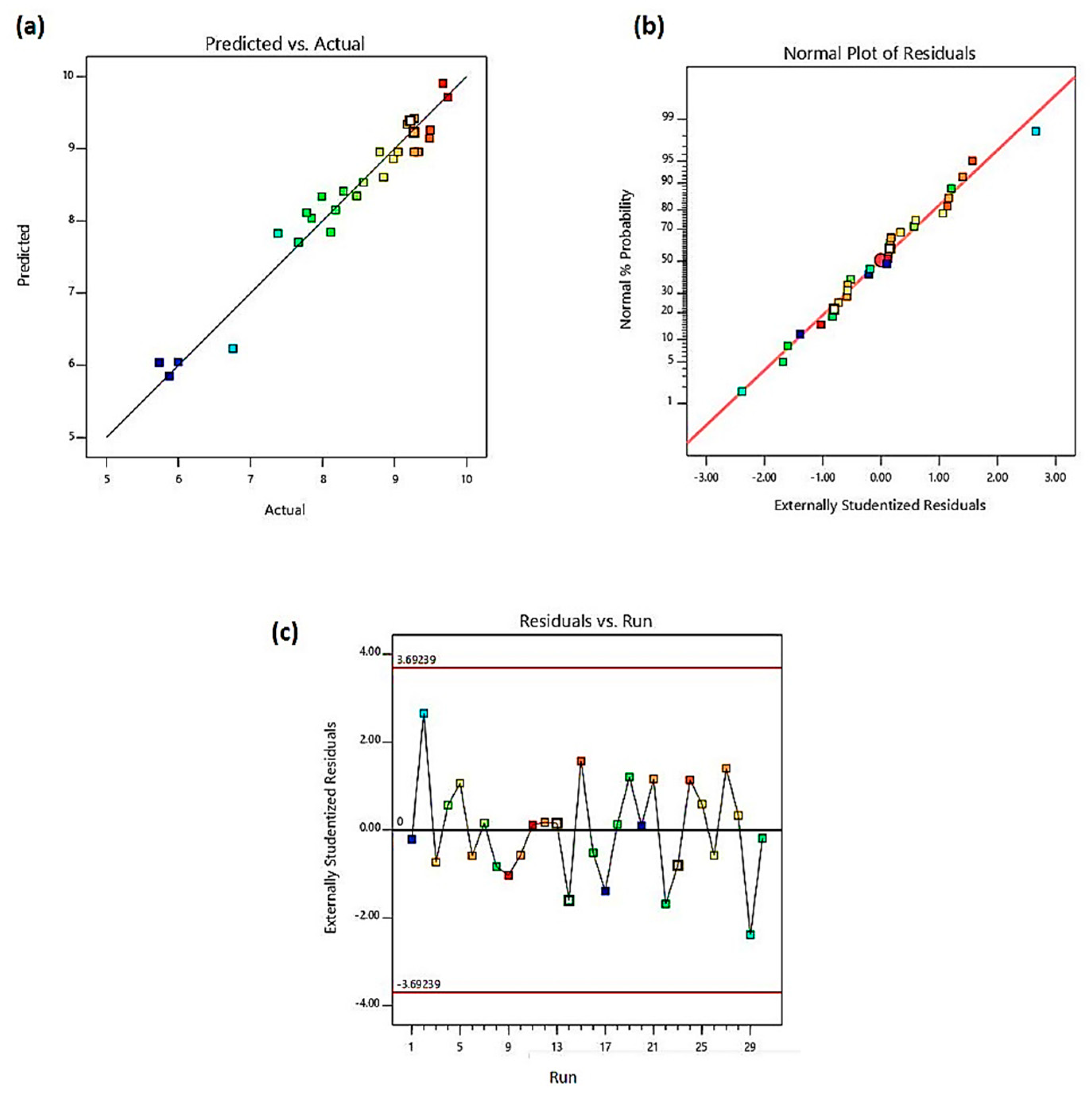
4.1.2. Diagnostic Plots

The predicted versus actual normality probability of residuals and the residuals versus run plots were used to evaluate the goodness-of-fit of the model. The good correlation between the actual and predicted mobility is depicted by the well distribution of the actual values to the predicted value line. The model’s pred-R² and adj-R² within 20% was found to be significantly acceptable. Meloun and Militky [50] suggested that a model could be used after a residual analysis has been performed, whereby the residual analysis is used to investigate outliers and detect influential observations. In Figure 3a, the diagnostic plot of the model with the pred-R² of 0.8736 showed that data points were close to the diagonal line. Likewise, in Figure 3b, the data points of the residuals followed a normal distribution as maximum plots are interlocked with the straight line. Furthering the residual analysis, Figure 3c showed a conformance to a random non-linear scattering trend along the run number and the absence of outliers. As such, there was no time-related variable lurking in the background. While the negative residual implies an over prediction, a positive residual indicates a low prediction. A plot close to the estimated regression line at zero (0) expounded on the exactness of prediction.

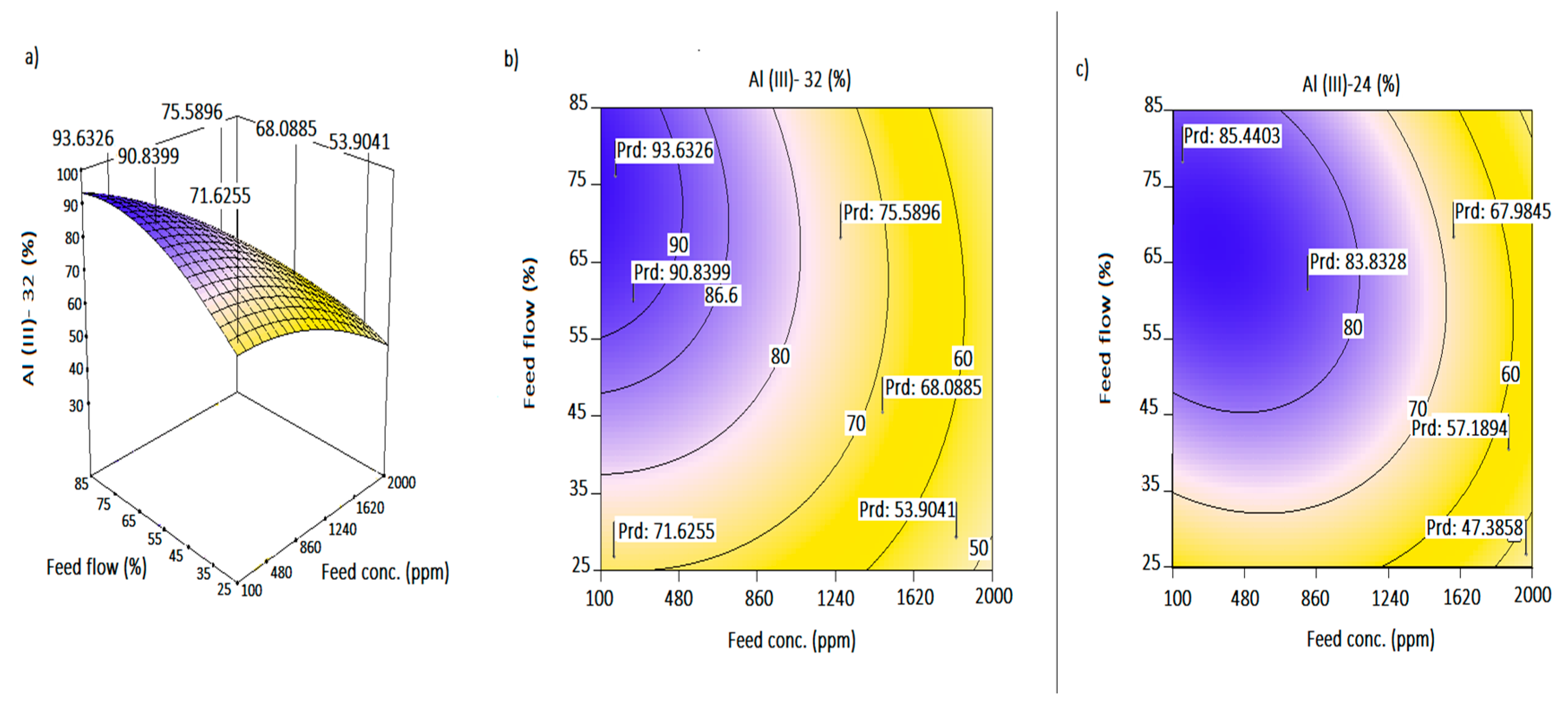
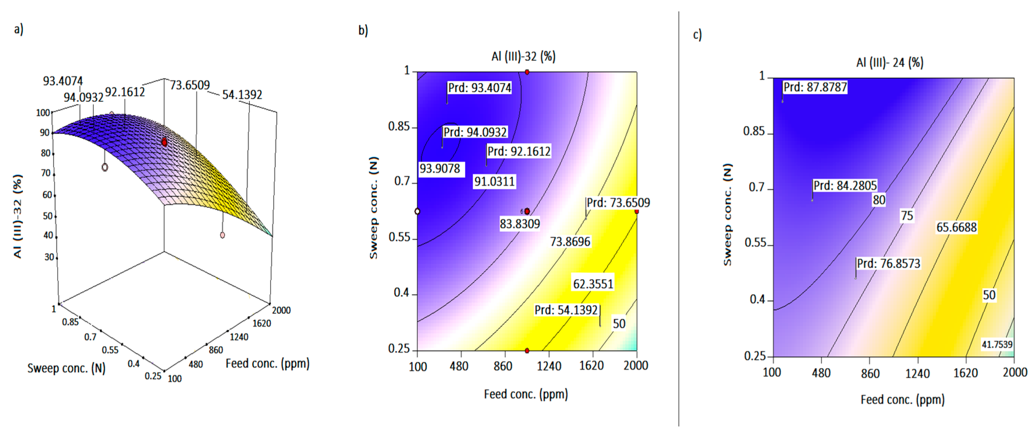
4.2. Combined Effects of Operating Parameters on the Response

Interpretation of the parametric interaction among the process variables was evaluated as the combined effects of feed concentration and feed flowrate (X₁X₂), as well as feed concentration and sweep concentration (X₁X₄). The three-dimensional plots (3D-plots) of the regression model were used for the graphical explanation of the interactions. Corresponding response surface plots (RSM) obtained from Equation (5) are presented in Figure 4a–c and Figure 5a–c. The degree of curvature on the 3D-plots depicts the levels of uncertainties attributed to the parametric interactions. Decision making using the RSM must take into account the variable effects on the response and the economic implications. For any good decision, there must be a balance between the considerations. Comparative Al transport at 24 h (Figure 4c and Figure 5c) and 32 h was undertaken using contour plot studies. Random flagged points (Prd) are shown on figures to illustrate the prediction points.

The concentration polarization effect due to bulk ion distribution at the membrane layer is dominant at a high feed concentration. Such an effect reduces selectivity and transmembrane flux [51]. In Figure 4a, increasing flowrate increased Al³⁺ transport at a decreasing feed concentration. At higher flowrates >55%, the Al-transport ranged between 80% and >90% for a feed range of 100 ≤ X₁ ≤ 1070 ppm at 32 h. An estimated 55–62% transport (Figure 4c) was also observed for decreasing feed concentration from 2000 ppm to about 1740 ppm at 24 h. As such, a higher feed flowrate does not translate into high mass transport at a high feed concentration. Recirculation of feed for a longer time increased the transport as long as the potential difference across the feed and sweep ends existed. A low transport of <60% was therefore reported between 1930 and 2000 ppm for a >75% flowrate at 32 h (Figure 4b). Under low to mid flow schemes (35–55%), one should expect an estimated 65% to >78.5% Al³⁺ transport from the feed phase with an operating feed concentration of 17,450–1340 ppm in 32 h.

The potential gradient to draw Al³⁺ increased with increasing sweep concentration. However, the negative impact of the increasing feed concentration was observed again in Figure 5a as the steepest point towards 2000 ppm. The mid to lowest Al-transport occurred at a lower sweep strength for sweep concentration of 0.25–0.38 N HCl. At that sweep concentration range, a transport of 42%–54% was observed for feed regions of 1800 to >1950 ppm. While attribution of the low Al transport to the drawing potential of the acid is valid, the bulk distribution at the membrane boundary at a high feed concentration could also be a great contributor to the reduced stoichiometric ion exchange. Above 0.48 N HCl, a feed range of 100–1550 ppm resulted in 70% to >90% target ion mobility (Figure 5b). An increasing operating concentration above 1N to maximize transport is not advisable. This can result in osmotic dehydration of membrane structure, loss of solute across sweep phase and osmotic transport [52]. The peak point on the curvature of Figure 5a, which reflected as the oval shape in Figure 4b, expounds on the high transport (93–94.1%) being in the region of 0.7–0.81 N HCl for a feed concentration ≤500 ppm. Observing Figure 5c at 24 h, an Al mobility of 60–68% is obtained for a 0.72–0.84 N and 1750–1980 ppm acid and acidic salt solution concentration, respectively. The high points (83–86%) for transport at 24 h occurred for a sweep concentration of 0.7–0.84 N and a feed concentration of 120–640 ppm. Therefore, any model generated for 24 h would predict within the range of responses observed in Figure 4c and Figure 5c (max = 90%). Interactions with sweep flowrate, which singularly has a linear-horizontal effect, and others such as X₁X₃ was excluded due to p > 0.05.

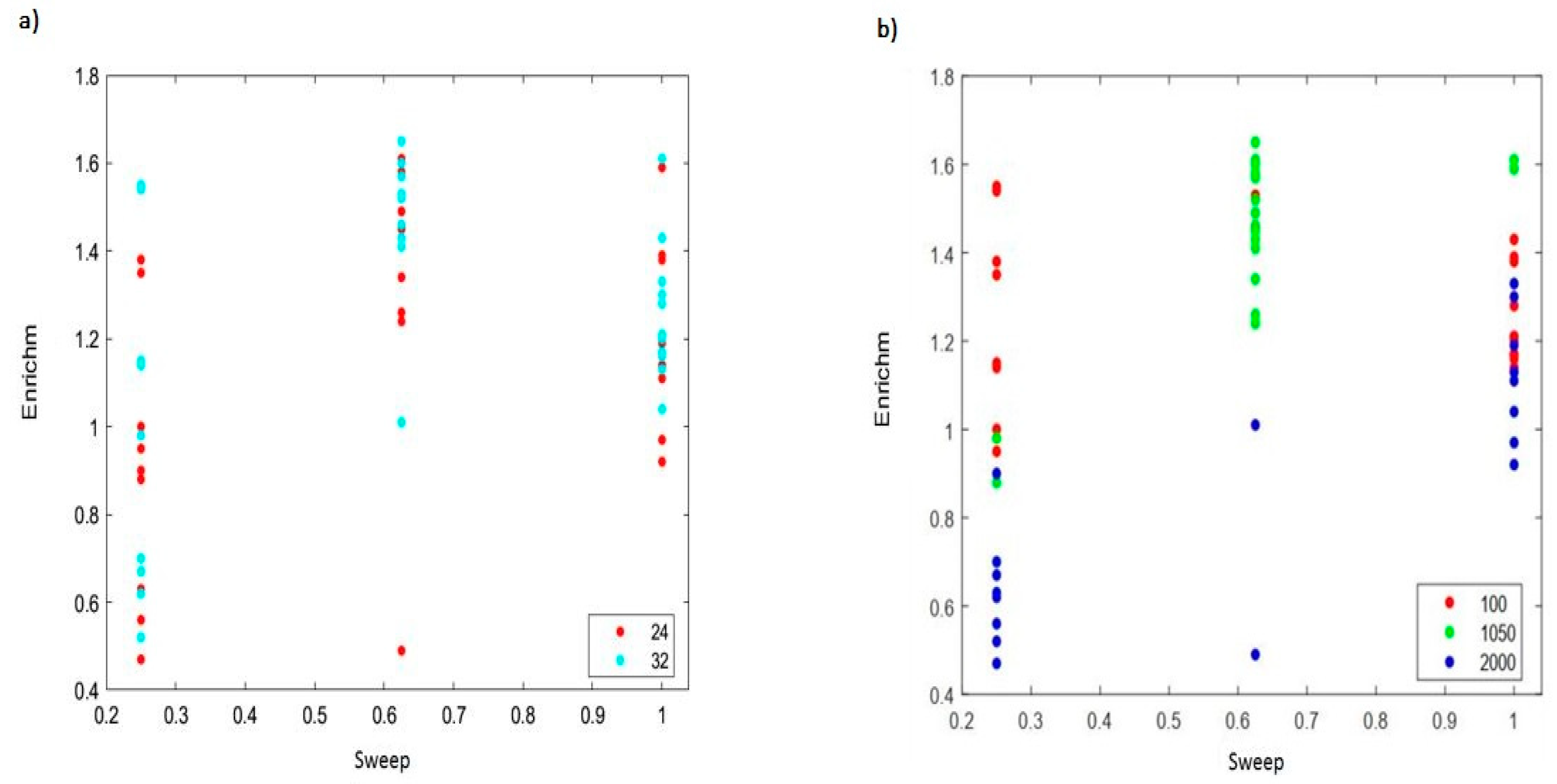
4.3. Enrichment Effect

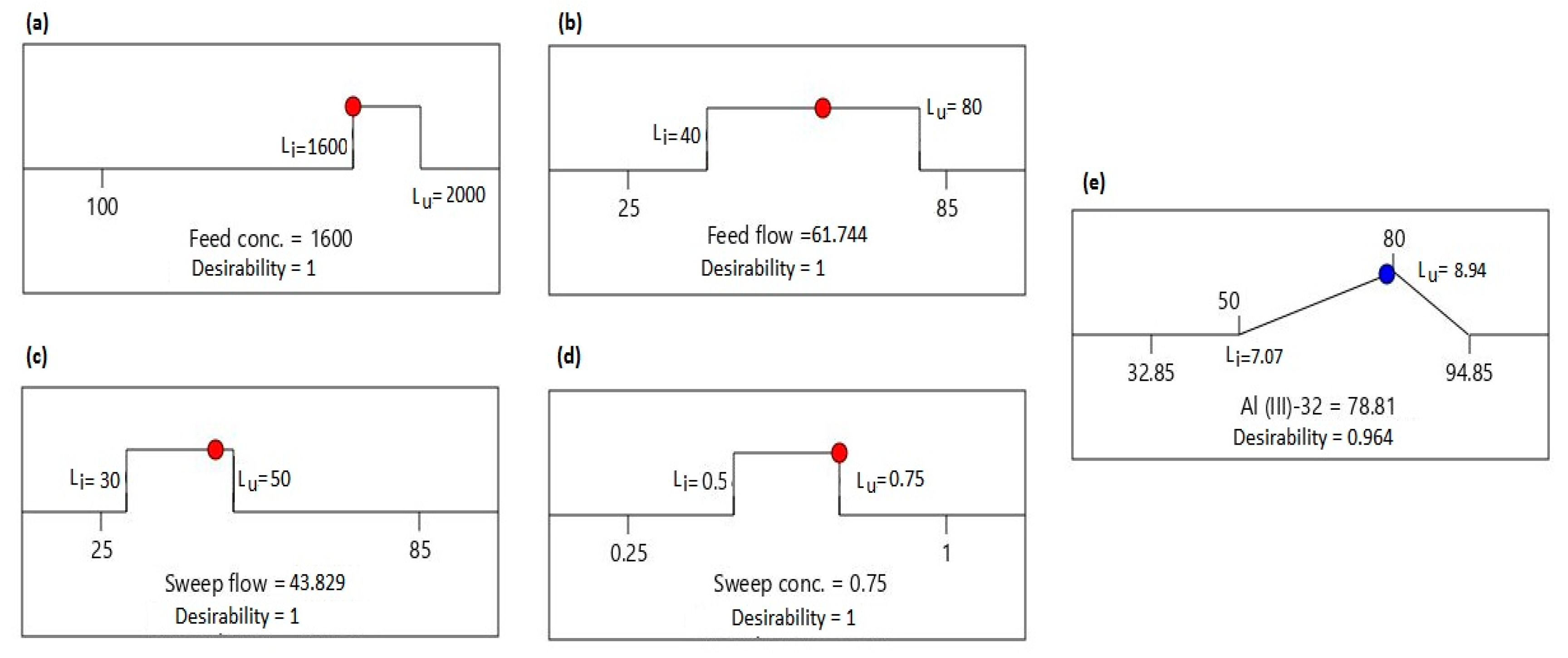
The enrichment effect of IED and its ability of the process concentrate transporting feed in the final sweep solution sets it apart from other processes. The good idea of enrichment at the sweep phase is clearly depicted by dividing Al in the sweep by the initial Al-concentration of the feed. Using 2–4 N sulfuric acid, and a 3:1 feed to sweep volume ratio, 2.4–3 times enrichment has been reported for Al recovery from water treatment residue using Nafion 117 [16,36]. Similarly, the enrichment of Al species at the feed and sweep phase was compared for 24 h and 32 h, respectively, for a 2:1 feed to sweep phase volume in Figure 6a,b. Depending on the other interactions (feed flow and sweep flow), a low feed concentration and low sweep concentration recorded an enrichment factor between 0.95 and 1.38 and 1.14 and 1.55 at 24 h and 32 h, respectively. Enrichment for a medium feed and sweep concentration was between 1.24 and 1.61 for 24 h and 1.41 and 1.65 at 32 h. Generally, the lower enrichments, <1.02, was within the operating conditions of medium feed–low sweep, high feed–low sweep and high feed–medium sweep concentrations. Furthermore, an observed lowest enrichment factor (0.47) was observed at a high feed and a low sweep concentration. Expectedly, a high sweep concentration should translate into high Al enrichment. However, comparing the enrichment ranges at 24 h and 32 h for low feed–low sweep concentrations and low feed–high sweep concentrations, dilution of the final sweep was evident at the high sweep concentration with enrichments of 1.13–1.39 at 24 h and 1.16–1.43 at 32 h. A seemingly progressive Al enrichment with respect to increasing acid (0.25–1 N) ensued at 2000 ppm. Without an overlapping enrichment at each time zone, Al³⁺ highs at 0.25, 0.625 and 1 N were 0.63, 0.90 and 1.19 for 24 h and 0.70, 1.01 and 1.33 for 32 h, respectively.

4.4. Desirability

The Desirability method is one of the most widely used non-linear programming techniques used to realize multi-objective optimization due to its simplicity and flexibility approach for each response. Responses (y_i) are transmuted into individual scale-free desirability values with a range of 0 ≤ d_i ≤ 1. A dimensionless desirability value of 0 indicates the response is outside of an acceptable region and the quality of the response is therefore undesirable. Having the response at its goal or target signifies that d_i = 1. In the Design Expert 11.0 worksheet, the goals of the desirability functions of the response are structured into minimum or maximum, within range or target and none. The goals of the factors only are set to exact values. The design variables are then chosen to maximize the overall desirability [53]:

$$D={(d_1\times d_2\times \dots d_n)}^{\frac{1}{n}}={({\displaystyle {{\displaystyle \prod }}_{i=1}^n}{d}_i)}^{\frac{1}{n}},$$

(6)

where n is the number of responses in the measure.

The feed concentration, feed flowrate, sweep flowrate and sweep concentration vary in the design range. In this numerical optimization of the counter flow IED system, the input variables were assessed to obtain a desired target Al transport >75%. Equal importance (3) and weight (1) are assigned for all the process variables and intent. Figure 7a–e shows the goals (in range for process variables), lower and upper limits (L_l and L_u), optimal value (red dotted for process variables and blue dotted for response) and desirability of the process variables and response. Out of a total of 51 solutions, the optimal parameters to achieve Al transport for feed concentration, feed flowrate, sweep flowrate and sweep concentration was 1600 ppm, 61.74%, 43.83% and 0.75 N, respectively, for the 32 h Al-transport model. The optimum results for maximum Al-transport is desirable with a combined desirability of 0.964, which is close to 1. To validate the results and performance of the counter flow IED system, five experimental runs at three-day intervals were conducted with optimal values of the process variables. An Al transport of 77.13% ± 4.19% was observed as compared to the set target of 80% and 78.81% predicted by the model. Setting an Al-permeation target at 70% for a 24 h experimental period, a difference of 1.23 was observed between the target and validation value at a desirability of 1 [41]. Although different targets were set for the two study zones, the closeness of the desirability to 1, the mechanism of the ion transport and the difference between the predicted and actual coefficient of variation plays an important role in the validation of optimum conditions.

5. Conclusions

The individual and combined effects of four process variables (feed concentration, feed flowrate, sweep flowrate and sweep concentration) on Al transport in a Nafion 117 membrane was studied using the FC-CCD model of RSM. The desirability approach was developed to carry out Al transport and optimization. The significant influences of the counter-flow IED system variables on Al transport were tested statistically by ANOVA. High adequacy precision ratio (22.839), act-R² (0.955) and adj-R² (0.936) values indicates the model at 32 h has a better goodness-of-fit and can navigate through the design space. The regression model for Al transport was obtained. A strong relation between the experimental and predicted results is shown by the 0.874 pred-R² and a standard deviation of 0.29. The interactive influence of the IED variables are illustrated and assessed in 3D surface and contour plots. An increase in feed concentration has a negative effect on Al transport. Positive impacts are observed with feed flowrate and sweep concentration. The impact of the sweep flowrate is not significant. Enrichment by Nafion 117 on the 2:1 by volume of the counter-flow IED system is between 0.47 and 1.65. The optimized parameters of the IED system are obtained to achieve the target transport using the desirability approach. Comparing the validated results to the predicted values by RSM, the optimized IED produces ±4.19 and shows that the RSM and desirability approach are reliable. The outcome of this research serves as a baseline to the Al-transport study for independent and interacting variables to determine operational periods for optimum recovery at the different time zones of 24 h and 32 h. Acidification of the residue for optimum recovery is reported at different pH values and it should be of future interest to investigate the effect of varied pH and other process variables on Al permeation.

References

1. Bobadilla, M.C.; Lorza, R.L.; García, R.E.; Gómez, F.S.; González, E.P.V. Coagulation: Determination of key operating parameters by multi-response surface methodology using desirability functions. Water 2019, 11, 398. [Google Scholar] [CrossRef] [Green Version]
2. Barrera-Díaz, C.E.; Balderas-Hernández, P.; Bilyeu, B. Electrocoagulation: Fundamentals and Prospectives. Electrochem. Water Wastewater Treat. 2018, 61–76. [Google Scholar] [CrossRef]
3. Kweinor Tetteh, E.; Rathilal, S. Application of Organic Coagulants in Water and Wastewater Treatment. Org. Polym. 2019, 13. [Google Scholar] [CrossRef] [Green Version]
4. Keeley, J.; Jarvis, P.; Judd, S.J. An economic assessment of coagulant recovery from water treatment residuals. Desalination 2012, 287, 132–137. [Google Scholar] [CrossRef]
5. Nesterenko, P.N. Ion Exchange-Overview, 3rd ed; Elsevier Inc.: Amsterdam, The Netherlands, 2018. [Google Scholar]
6. Keeley, J.; Jarvis, P.; Judd, S.J. Coagulant Recovery from Water Treatment Residuals: A Review of Applicable Technologies. Crit. Rev. Environ. Sci. Technol. 2014, 44, 2675–2719. [Google Scholar] [CrossRef] [PubMed] [Green Version]
7. Pawlowski, S.; Crespo, J.G.; Velizarov, S. Profiled Ion Exchange Membranes: A Comprehensible Review. Int. J. Mol. Sci. 2019, 20, 165. [Google Scholar] [CrossRef] [PubMed] [Green Version]
8. Hassanvand, A.; Wei, K.; Talebi, S.; Chen, G.; Kentish, S. The Role of Ion Exchange Membranes in Membrane Capacitive Deionisation. Membranes 2017, 7, 54. [Google Scholar] [CrossRef] [Green Version]
9. Hagesteijn, K.F.L.; Jiang, S.; Ladewig, B.P. A review of the synthesis and characterization of anion exchange membranes. J. Mater. Sci. 2018, 53, 11131–11150. [Google Scholar] [CrossRef] [Green Version]
10. Bdiri, M.; Dammak, L.; Larchet, C.; Hellal, F.; Porozhnyy, M.; Nevakshenova, E.; Pismenskaya, N.; Nikonenko, V. Characterization and cleaning of anion-exchange membranes used in electrodialysis of polyphenol-containing food industry solutions; comparison with cation-exchange membranes. Sep. Purif. Technol. 2019, 210, 636–650. [Google Scholar] [CrossRef]
11. Xu, T. Ion exchange membranes: State of their development and perspective. J. Membr. Sci. 2005, 263, 1–29. [Google Scholar] [CrossRef]
12. Ran, J.; Wu, L.; He, Y.; Yang, Z.; Wang, Y.; Jiang, C.; Ge, L.; Bakangura, E.; Xu, T. Ion exchange membranes: New developments and applications. J. Membr. Sci. 2017, 522, 267–291. [Google Scholar] [CrossRef]
13. Luo, T.; Abdu, S.; Wessling, M. Selectivity of ion exchange membranes: A review. J. Membr. Sci. 2018, 555, 429–454. [Google Scholar] [CrossRef]
14. Sarkar, S.; SenGupta, A.K.; Prakash, P. The Donnan Membrane Principle: Opportunities for Sustainable Engineered Processes and Materials. Environ. Sci. Technol. 2010, 44, 1161–1166. [Google Scholar] [CrossRef] [PubMed]
15. Vanoppen, M.; Stoffels, G.; Demuytere, C.; Bleyaert, W.; Verliefde, A.R.D. Increasing RO efficiency by chemical-free ion-exchange and Donnan dialysis: Principles and practical implications. Water Res. 2015, 80, 59–70. [Google Scholar] [CrossRef] [PubMed]
16. Prakash, P.; SenGupta, A.K. Selective Coagulant Recovery from Water Treatment Plant Residuals Using Donnan Membrane Process. Environ. Sci. Technol. 2003, 37, 4468–4474. [Google Scholar] [CrossRef]
17. Kim, D.; Judy, J.W. Analysis of Donnan-dialyzer irreproducibility and experimental study of a microfluidic parallel-plate membrane-separation module for total analysis systems. J. Membr. Sci. 2014, 460, 148–159. [Google Scholar] [CrossRef]
18. Çengeloǧlu, Y.; Kir, E.; Ersöz, M. Recovery and concentration of Al(III), Fe(III), Ti(IV), and Na(I) from red mud. J. Colloid Interface Sci. 2001, 244, 342–346. [Google Scholar] [CrossRef]
19. Çengeloǧlu, Y.; Kir, E.; Ersoz, M.; Buyukerkek, T.; Gezgin, S. Recovery and concentration of metals from red mud by Donnan dialysis. Colloids Surf. A Physicochem. Eng. Asp. 2003, 223, 95–101. [Google Scholar] [CrossRef]
20. Sonoc, A.C.; Jeswiet, J.; Murayama, N.; Shibata, J. A study of the application of Donnan dialysis to the recycling of lithium ion batteries. Hydrometallurgy 2018, 175, 133–143. [Google Scholar] [CrossRef]
21. Ping, Q.; Abu-Reesh, I.M.; He, Z. Boron removal from saline water by a microbial desalination cell integrated with donnan dialysis. Desalination 2015, 376, 55–61. [Google Scholar] [CrossRef]
22. Okada, T.; Xie, G.; Gorseth, O.; Kjelstrup, S.; Nakamura, N.; Arimura, T. Ion and water transport characteristics of Nafion membranes as electrolytes. Electrochim. Acta 1998, 43, 3741–3747. [Google Scholar] [CrossRef]
23. Miyoshi, H. Diffusion coefficients of ions through ion excange membrane in Donnan dialysis using ions of different valence. J. Membr. Sci. 1998, 141, 101–110. [Google Scholar] [CrossRef]
24. Pessoa-Lopes, M.; Crespo, J.G.; Velizarov, S. Arsenate removal from sulphate-containing water streams by an ion-exchange membrane process. Sep. Purif. Technol. 2016, 166, 125–134. [Google Scholar] [CrossRef]
25. Zhao, B.; Zhao, H.; Ni, J. Arsenate removal by Donnan dialysis: Effects of the accompanying components. Sep. Purif. Technol. 2010, 72, 250–255. [Google Scholar] [CrossRef]
26. Velizarov, S. Transport of arsenate through anion-exchange membranes in Donnan dialysis. J. Membr. Sci. 2013, 425–426, 243–250. [Google Scholar] [CrossRef]
27. Wiśniewski, J.A.; Kabsch-Korbutowicz, M.; Łakomska, S. Ion-exchange membrane processes for Br- and BrO3-Ion removal from water and for recovery of salt from waste solution. Desalination 2014, 342, 175–182. [Google Scholar] [CrossRef]
28. Marzouk, I.; Dammak, L.; Chaabane, L.; Hamrouni, B. Optimization of Chromium (Vi) Removal by Donnan Dialysis. Am. J. Anal. Chem. 2013, 4, 306–313. [Google Scholar] [CrossRef] [Green Version]
29. Turki, T.; Amor, M.B. Nitrate removal from natural water by coupling adsorption and Donnan dialysis. Water Sci. Technol. Water Supply 2017, 17, 771–779. [Google Scholar] [CrossRef]
30. Oehmen, A.; Valerio, R.; Llanos, J.; Fradinho, J.; Serra, S.; Reis, M.A.M.; Crespo, J.G.; Velizarov, S. Arsenic removal from drinking water through a hybrid ion exchange membrane—Coagulation process. Sep. Purif. Technol. 2011, 83, 137–143. [Google Scholar] [CrossRef]
31. Ayyildiz, H.F.F.; Kara, H. Boron removal by ion exchange membranes. Desalination 2005, 180, 99–108. [Google Scholar] [CrossRef]
32. Szczepański, P.; Szczepańska, G. Donnan dialysis—A new predictive model for non−steady state transport. J. Membr. Sci. 2017, 525, 277–289. [Google Scholar] [CrossRef]
33. Agarwal, C.; Chaudhury, S.; Pandey, A.K.; Goswami, A. Kinetic aspects of Donnan dialysis through Nafion-117 membrane. J. Membr. Sci. 2012, 415–416, 681–685. [Google Scholar] [CrossRef]
34. Agarwal, C.; Goswami, A. Nernst Planck approach based on non-steady state flux for transport in a Donnan dialysis process. J. Membr. Sci. 2016, 507, 119–125. [Google Scholar] [CrossRef]
35. Wang, Q.; Lenhart, J.J.; Walker, H.W. Recovery of metal cations from lime softening sludge using Donnan dialysis. J. Membr. Sci. 2010, 360, 469–475. [Google Scholar] [CrossRef]
36. Prakash, P.; Hoskins, D.; SenGupta, A.K. Application of homogeneous and heterogeneous cation-exchange membranes in coagulant recovery from water treatment plant residuals using Donnan membrane process. J. Membr. Sci. 2004, 237, 131–144. [Google Scholar] [CrossRef]
37. Adesina, O.A.; Abdulkareem, F.; Yusuff, A.S.; Lala, M.; Okewale, A. Response surface methodology approach to optimization of process parameter for coagulation process of surface water using Moringa oleifera seed. S. Afr. J. Chem. Eng. 2019, 28, 46–51. [Google Scholar] [CrossRef]
38. Tetteh, E.; Amano, K.O.A.; Asante-Sackey, D.; Armah, E. Response Surface Optimisation of Biogas Potential in Co-Digestion of Miscanthus Fuscus and Cow Dung. Int. J. Technol. 2018, 9, 944. [Google Scholar] [CrossRef] [Green Version]
39. John, B.D.; King, P.; Prasanna, K.Y. Optimization of Cu (II) biosorption onto sea urchin test using response surface methodology and artificial neural networks. Int. J. Environ. Sci. Technol. 2019, 16, 1885–1896. [Google Scholar] [CrossRef]
40. Taran, M.; Aghaie, E. Designing and optimization of separation process of iron impurities from kaolin by oxalic acid in bench-scale stirred-tank reactor. Appl. Clay Sci. 2015, 107, 109–116. [Google Scholar] [CrossRef]
41. Asante-Sackey, D.; Rathilal, S.; Pillay, L.; Tetteh, E.K. Effect of ion exchange dialysis process variables on aluminium permeation using response surface methodology. Environ. Eng. Res. 2019. [Google Scholar] [CrossRef]
42. Kleijnen, J.P.C. Response surface methodology. Int. Ser. Oper. Res. Manag. Sci. 2015, 216, 81–104. [Google Scholar]
43. Sahoo, P.; Barman, T.K. ANN modelling of fractal dimension in machining. Mechatron. Manuf. Eng. 2012, 159–226. [Google Scholar] [CrossRef]
44. Iqbal, M.; Iqbal, N.; Bhatti, I.A.; Ahmad, N.; Zahid, M. Response surface methodology application in optimization of cadmium adsorption by shoe waste: A good option of waste mitigation by waste. Ecol. Eng. 2016, 88, 265–275. [Google Scholar] [CrossRef]
45. Tetteh, E.K.; Rathilal, S. Effects of a polymeric organic coagulant for industrial mineral oil wastewater treatment using response surface methodology (Rsm). Water SA 2018, 44, 155–161. [Google Scholar] [CrossRef] [Green Version]
46. Owolabi, R.U.; Usman, M.A.; Kehinde, A.J. Modelling and optimization of process variables for the solution polymerization of styrene using response surface methodology. J. King Saud Univ. Eng. Sci. 2018, 30, 22–30. [Google Scholar] [CrossRef] [Green Version]
47. Siegel, A.F. Chapter 12-Multiple Regression: Predicting One variable from several others. Pract. Bus. Stat. 2012, 347–416. [Google Scholar] [CrossRef]
48. Nair, A.T.; Ahammed, M.M. The reuse of water treatment sludge as a coagulant for post-treatment of UASB reactor treating urban wastewater. J. Clean. Prod. 2015, 96, 272–281. [Google Scholar] [CrossRef]
49. Aerts, S.; Haesbroeck, G.; Ruwet, C. Multivariate coefficients of variation: Comparison and influence functions. J. Multivar. Anal. 2015, 142, 183–198. [Google Scholar] [CrossRef]
50. Meloun, M.; Militký, J. Statistical analysis of multivariate data. Stat. Data Anal. 2011, 151–403. [Google Scholar] [CrossRef]
51. Luis, P. Introduction. Fundam. Model. Memb. Syst. 2018, 1–23. [Google Scholar] [CrossRef]
52. Davis, T.A. Donnan Dialysis. In Membrane Processes; Academic Press: Cambridge, MA, USA, 2000; Volume 2, pp. 1701–1707. [Google Scholar]
53. Mohapatra, T.; Sahoo, S.S.; Padhi, B.N. Analysis, prediction and multi-response optimization of heat transfer characteristics of a three fluid heat exchanger using response surface methodology and desirability function approach. Appl. Therm. Eng. 2019, 151, 536–555. [Google Scholar] [CrossRef]
Figure 1. Conceptual design of an ion exchange dialysis (IED) rig.
Processes 08 00160 g001
Figure 2. Schematic flow for Al-transport study.
Processes 08 00160 g002
Figure 3. (a) Predicted versus actual values plot; (b) normal probability plot; (c) residual versus total run plot.
Processes 08 00160 g003
Figure 4. (a) Response surface plot for the interactive effect of feed flow and feed concentration at 32 h; (b,c) contour plots of Al transport as a function of feed flow and feed concentration at 32 h and 24 h, respectively.
Processes 08 00160 g004
Figure 5. (a) Response surface plot for the interactive effect of sweep concentration and feed concentration at 32 h; (b,c) contour plots of Al-transport as a function of feed flow and feed concentration at 32 h and 24 h, respectively.
Processes 08 00160 g005
Figure 6. (a) Enrichment factor plot for 24 and 32 h. (b) Enrichment plot based on feed concentration.
Processes 08 00160 g006
Figure 7. (a) Optimal value for the feed concentration for 32 h; (b) Optimal value for the feed flowrate for 32 h; (c) Optimal value for the sweep flowrate for 32 h; (d) Optimal value for the sweep concentration for 32 h; (e) Optimum results for Al transport for 32 h.
Processes 08 00160 g007