
Conceptual Design of a Negative Emissions Polygeneration Plant for Multiperiod Operations Using P-Graph


1
Department of Chemical and Environmental Process Engineering, Budapest University of Technology and Economics, 1111 Budapest, Hungary
2
Department of Computer Science and Systems Technology, University of Pannonia, 8200 Veszprém, Hungary
3
Chemical Engineering Department, De La Salle University, Manila 0922, Philippines
4
Artificial Intelligence National Laboratory, Széchenyi István University, 9026 Győr, Hungary
*
Author to whom correspondence should be addressed.
Processes 2021, 9(2), 233; https://doi.org/10.3390/pr9020233
Submission received: 28 December 2020
/
Revised: 16 January 2021
/
Accepted: 21 January 2021
/
Published: 27 January 2021
(This article belongs to the Special Issue Multi-Period Optimization of Sustainable Energy Systems)
Abstract
:Reduction of CO2 emissions from industrial facilities is of utmost importance for sustainable development. Novel process systems with the capability to remove CO2 will be useful for carbon management in the future. It is well-known that major determinants of performance in process systems are established during the design stage. Thus, it is important to employ a systematic tool for process synthesis. This work approaches the design of polygeneration plants with negative emission technologies (NETs) by means of the graph-theoretic approach known as the P-graph framework. As a case study, a polygeneration plant is synthesized for multiperiod operations. Optimal and alternative near-optimal designs in terms of profit are identified, and the influence of network structure on CO2 emissions is assessed for five scenarios. The integration of NETs is considered during synthesis to further reduce carbon footprint. For the scenario without constraint on CO2 emissions, 200 structures with profit differences up to 1.5% compared to the optimal design were generated. The best structures and some alternative designs are evaluated and compared for each case. Alternative solutions prove to have additional practical features that can make them more desirable than the nominal optimum, thus demonstrating the benefits of the analysis of near-optimal solutions in process design.
1. Introduction
Technological development and economic growth have led to a rise in the emissions of CO2 derived from the combustion of fuels. Global carbon emissions increased from 19.7 Gt CO2 eq./y in 1970 to 37.3 Gt CO2 eq./y in 2010. In the same period, CO2 emissions from fuels and industrial processes increased by 17.05 Gt CO2 eq./y, representing 97% of the total growth [1]. However, there have been recent efforts to mitigate the environmental problems resulting from the emissions of greenhouse gases (GHGs), such as the reduction of pollutants during product generation, the enhancement of process efficiencies to reduce the consumption of resources, or the integration of processes to save energy. An example of a technology for reducing GHG emissions is polygeneration, which is defined as the generation of multiple utilities and products from a single facility; it allows reductions in fuel consumption and GHG emissions by capitalizing on opportunities for process integration when producing multiple outputs [2].
Furthermore, the deployment of negative emission technologies (NET) has been proposed to indirectly decrease the net amount of CO2 released to the environment. NETs are defined as methods that result in a reduction of the level of GHGs through their permanent removal from the atmosphere [3]. Large-scale use of NETs will be needed in the coming decades to minimize temperature rise throughout the remainder of the 21st Century [4]. Several initiatives have been developed in this field and can be classified in six general categories [5]: Afforestation and reforestation, land management to increase and fix carbon in soils, bioenergy production with carbon capture and storage (BECCS), enhanced weathering, direct capture of CO2 from ambient air with CO2 storage (DACCS), and ocean fertilization to increase its CO2 absorption capability. In addition to well-known NETs, new concepts have also been proposed recently. For instance, Davies et al. [6], proposed a NET concept based on the integration of reverse osmosis (RO) process with electrolysis; in this scheme, the waste brine produced during the RO step is processed in an electrolytic cell with a gas diffusion anode (EGDA) to transform the MgCl2 in the waste brine into Mg(OH)2,. The resulting waste brine is thus slightly alkaline and is capable of absorbing CO2 when released in the ocean. The term Davies process will be used to refer to this concept from hereon.
The Davies process was originally envisioned as a standalone NET [6]. Tan et al. [7] proposed its integration in a flexible polygeneration plant that employs RO to produce water, and presented a mathematical programming model for the optimal synthesis of the network. The Davies process is used as part of a power-to-X scheme to take advantage of cyclic variations in electricity price and product demand. Such integration requires additional capital investment during early design stages, and an assessment of various profitability scenarios should be considered. This evaluation for the design of processes can be performed employing a multiperiod optimization approach.
Multiperiod optimization is beneficial over separate single-period optimizations. The improvement in the optimal results has been demonstrated in multiple areas, e.g., public transport optimization [8], gas transmission network design [9], or waste recycling [10]. The decision of existence and partial operation of units in the different periods within multiperiod consideration constitutes a combinatorial problem by nature, and generally results in a mixed integer linear programming (MILP) or mixed integer nonlinear programming (MINLP) model. Conventional solution methods are only capable of generating a single solution for this kind of model. Solutions can be obtained with available deterministic solvers for limited-size problems [11], or by heuristic or nondeterministic approaches [12] for larger problems.
The unique solution obtained may not be enough for the design engineers to make a decision, because of the inherent simplifications of the model and the design aspects not considered in it [13]. The importance of generating multiple near-optimal solutions to enable further analysis of the synthesis problem was demonstrated by a P-graph based approach of Orosz and Friedler [14] for heat exchanger network synthesis.
Generation of alternative designs can also be performed by introducing integer cut constraints in the MILP or MINLP problem [13]. Conversely, P-graph is a powerful and versatile framework for rigorous process network synthesis (PNS) that is especially useful for handling combinatorial aspects of design problems [15]. This approach permits the systematic generation of the best solution and a set of near-optimal alternatives by efficiently reducing the size of the optimization problem.
This work develops an alternative graph-theoretic approach for the synthesis of a polygeneration plant with an integrated Davies process for multiperiod operation. The proposed method relies on the tools of the P-graph approach, which permits the effective identification of the n-best alternatives for the plant design. In this work, storage tanks can be used between periods to store byproducts to achieve a certain stabilization of the network when fluctuating resources are employed by means of a power-to-X system. The combinatorial tools of the P-graph framework [16] permit the identification of the most cost-effective network in consideration of various operating conditions. Moreover, near-optimal design networks are also generated which may potentially be more practical to implement.
2. Problem Statement
The synthesis problem addressed in this paper starts with the definition of the sets P, R and O. The set P includes all the industrial services or products to be generated. Conversely, the set R comprises candidate raw materials that can be transformed into products or intermediate materials. The definition of sets P and R requires the association of the elements of these sets with their individual prices, availabilities and demands. On the other hand, the set O contains the candidate operating units that are considered for performing the transformation of materials within the process. The technical coefficients, emission factors and cost estimator functions of the operating units in O are assumed to be known. Additionally, the time horizon is defined and divided into K periods. Altogether with the number of periods K, the length of each period is also specified.
The objective is to identify the set of potential alternative designs that satisfy the demand of products P, and to determine the operating state for the units in the different periods for each network. The identification of the alternative designs is performed by maximizing the profit of the operation, considering as decision variables the topology of the networks, the capacity of units involved in them, and the working capacity for each period. Therefore, this set of alternatives comprises the optimal design in terms of profit, as well as a set of near-optimal designs that provide additional information for decision making. Furthermore, removal of CO2 by inclusion of NETs in the network is considered as one of the outputs of the system.
3. Methodology
3.1. P-Graph Framework
The P-graph framework is a graph-theoretic approach that can deal with problems of combinatorial nature in a systematic way. P-graph relies on a bipartite graph with O-type and M-type nodes that represent process units and process streams, respectively. The methodology has its basis on three main cornerstones: The P-graph representation, a set of five axioms, and a set of combinatorial algorithms. The P-graph representation is capable of unambiguously depicting a process, thus allowing the realization of the combinatorial transformations required for synthesizing multiperiod operations. Figure 1 shows the representation of an operating unit (boiler) that employs purified water and biomass for the generation of vapor. The streams are represented by M-type vertices (i.e., circles), whereas the operation is depicted by an O-type vertex (i.e., horizontal bar). Figure 1 also describes the different subtypes of M-type vertices, or circular nodes, commonly employed in P-graph representation.
The set of algorithms used in P-graph allows for effective solution of PNS problems. Maximal structure generation (MSG) enables the algorithmic generation of a rigorous superstructure (referred to as the maximal structure) from individually specified process units. MSG connects process units based on common streams, and the resulting maximal structure is both complete and nonredundant. This algorithm eliminates the risk of human error that may occur in heuristically specified superstructures [17]. Next, solution structure generation (SSG) allows the enumeration of all combinatorially or structurally feasible networks in a PNS problem [18]. Local search can be done within each of these structures to allow a range of different solutions to be evaluated by the designer. Finally, accelerated branch-and-bound (ABB) utilizes PNS logic to allow rapid optimization via drastic reduction in search space [19].
P-graph was originally developed to solve steady-state PNS problems. The development of a multiperiod model in P-graph was initially proposed by Heckl et al. [20] by representing the problem as a superstructure that separates the capital costs from the operating costs. This structure can consider constraints for multiple periods, such as the maximum capacities of operating units, or availabilities and demands of materials. This representation of the problem is generated by replicating the vertices that are involved in multiperiodic operation. The subsequent interconnection of these nodes generates a superstructure that depicts all the operations for all periods.
Aviso et al. [21] developed a formulation for optimizing multiperiod energy systems considering part-load operating limits. An example of the implementation of this method in the software P-Graph Studio [22] involving storage between periods and waste treatment is presented by Bertok and Bartos [23] for the design of a vinyl chloride production plant. Recently, Bertok and Bartos [24] introduced the use of multiperiod process optimization by means of P-graph for designing distribution grids for renewable energy.
3.2. Illustrative Example
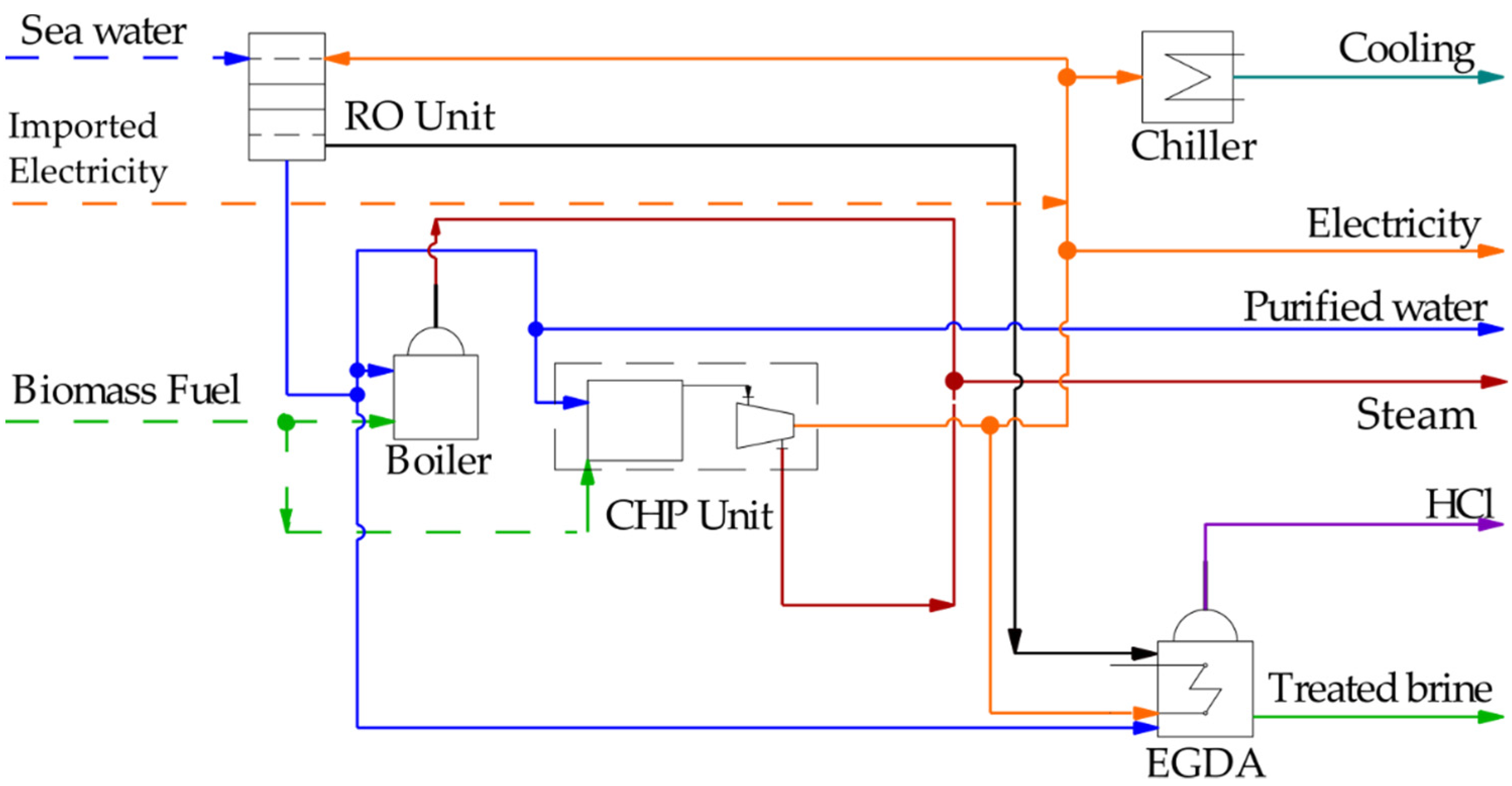
A small illustrative example with four periods per day (six hours per period) is solved here. The graphical representation of the initial problem is presented in Figure 2. A plant that generates industrial utilities for heating, cooling, electric power, and fresh water needs to be synthesized. This plant has the objective of producing the set of industrial services according to the requirements of the main process; thus, the demands of heating, cooling, as well as the requirements of electricity change for each period. Additionally, the price of electrical power also exhibits variations during the day due to spot market fluctuations.
There are two candidate operations for producing heating in the form of steam, the first being a boiler that employs biomass and purified water to generate steam. The second is a combined heat and power module with heat recovery (CHP Unit), which can also be used as a source of electricity. The demand for electricity can also be fulfilled by importing it from the external grid. Because of the geographical location, the only water source is the sea. This water can be treated by means of a RO unit, to obtain a stream of purified water and a stream of concentrated brine. The inclusion of EGDA to produce treated brine is also considered here; this slightly alkaline treated brine will absorb CO2 and thus generate negative emissions when discharged into the sea. The HCl derived from this process is sold as a byproduct. Finally, cooling capacity can be generated by a refrigeration cycle (termed here as Chiller), whose only feed is assumed to be electricity. The payout period for the amortization of operating units is assumed to be 10 years, while the prices of utilities and demands for each period are considered as shown in Table 1.
Table 2 presents the mass and energy balances and the cost parameters for the plausible operation units depicted in Figure 2. These values are based on the case study presented by Tan et al. [7]. Environmental impact and release of GHG (represented uniquely by CO2) were assessed by assuming that they are directly proportional to the capacity of the boiler, the CHP unit, and the imported electricity. Emission factors for these units were employed to estimate the amount of CO2 generated per unit of energy [25]. Capital cost of the operating units is estimated here as a function of the size of the units by means of a piecewise linear function with fixed and variable cost components.
The possibility of storing materials to be employed through the operation is also evaluated in the synthesis problem. The illustrative example only considers the storage of water; however, Table 3 shows the cost parameters and constraints considered for all storage units used in this work.
The solution of this illustrative example begins by representing the conventional problem structure (Figure 2) as a P-graph. Figure 3 compares the conventional representation of the structure to its P-graph representation. In order to facilitate the comparison, the conventional form previously shown in Figure 2 is presented again in Figure 3a. In Figure 3b, the streams of the conventional representation are transformed into circles (M-type vertices) and its blocks are transformed into horizontal bars (O-type vertices). The streams introduced in the process from an external source that are represented by discontinuous lines in Figure 3a, are regarded as raw materials in Figure 3b. On the other hand, the industrial services required are depicted as product nodes. The remaining materials are represented as intermediate materials. Figure 3b is the P-graph representation of a single period.
Using the implementation of the P-graph framework for multiperiod design proposed by Heckl et al. [20], the synthesis problem is depicted as the maximal structure shown in Figure 4. In this figure, the structure for a single period in Figure 3b is replicated four times to represent the operational conditions for each period. These structures can be seen in Figure 4 drawn with black lines and enclosed with a broken line.
These four structures represent different operating states of the plant. Then, they are connected to fictitious operating units that represent the maximum available installed capacity for each unit. These units are shown in blue in the left-hand side of the figure and are termed as capacity nodes. These blue nodes are used to estimate capital cost.
The capacity node is constrained by the highest capacity required for the corresponding unit in consideration of the requirements in the individual periods. Moreover, the orange lines in the right-hand side of the diagram represent the relation between periods given by the storage of water. Since the storage units are also regarded as plausible units during synthesis, a horizontal bar is required to depict their maximum capacity and the fixed cost of the actual storage tanks. This fictitious unit is termed as storage capacity node.
Implementation in previous works [20,21] indicate that the values of the arcs that connect the fixed units with the blue material nodes are calculated as the length of the period divided by the total time of analysis. This step ensures that the maximal capacity delivered by the capacity node is at least as big as the maximum capacity required for operation. However, since the maximum capacity of the storage units is not a flow but a stock that represents the maximum stored material, the value of the arcs that connect the storage capacity nodes with their corresponding operation nodes is defined as one.
For cyclic operations, it is necessary that the initial load of the storage units (i.e., material stored from the previous day), be available again in the tank when the day ends. For this, the operating unit “initial storage recovery” is introduced. This operation assures the availability of initial load by relating the purified water generated in the last period to the “Initial load” vertex. This scheme ends in a loop when connected with the storage operation in the first period. Additionally, the maximum amount of the material node “Initial load” is constrained to zero, thus ensuring that material accumulated in the last period matches the initial load demanded for the next day. As previously mentioned, the illustrative example only considers storage of water; therefore, Figure 4 only exhibits one scheme of storage units. The same principle can be readily extended to other forms of storage. A similar set of vertices is needed to depict the units involved in the evaluation of every plausible storage option.
Implementation of the algorithm ABB effectively generates the optimal solution along with a wide range of near-optimal solutions. For the illustrative example, only the best structure in terms of profit is presented. The solutions generated in this work describe the maximal capacity of the equipment to be installed in the plant, as well as the capacity at which they work in each period. Thus, they represent flexible designs capable of operating in different ways to meet the demand. The operating constraints considered here are mainly the time-varying demands and costs. Additional constraints such as those based on minimum part-load operating states [26] will be addressed in future work. Figure 5 depicts the best structure obtained for the synthesis of a multiperiod polygeneration plant in the illustrative example. For this particular solution, all operating units are installed, and therefore the blue part on the left-hand side of the picture remains the same. Nonetheless, the operation suggested by the answer recommends the part-load operation of some of the operating units during the day. In Figure 5, operating units that are not active are presented in grey for the period in which they are not employed. On the other hand, the horizontal bars of the active operating units are presented in green. Moreover, the degree of use of the active operating units for each period is indicated by the partially filled horizontal bars. For instance, the boiler is deployed at its maximum capacity during the first period, this is represented as a full green bar; then, it is operated at half capacity during period 2, consequently its horizontal bar is filled at 50%.
The process and operation policy depicted on the structure illustrated in Figure 5 yield a profit of EUR 1408.19/day. It can be seen that the operating units RO and EGDA are operated at full capacity all day. The operation of the chiller answers directly to the demand for cooling necessary to complete the process. This operation is inactive during period 1, and then it gradually increases its production according to the rise in the demand until it reaches 100% in period 4. The boiler is inactive during period 3 since steam demand is low and the CHP Unit can fulfill it. Furthermore, the boiler only needs to be active at 50% of its capacity during period 2. In period 4, however, it is fully active since the CHP is not employed. The latter is not necessary because the demand of electricity becomes lower and it is cheaper to import it from the grid instead of producing it. The tank of water starts the day at almost full capacity (close to 96%) and it is emptied during period 1. It remains empty up to the beginning of period 2, is filled again to its maximum capacity during period 3, and thus starts period 4 completely full. During period 4, only a small fraction is depleted, recovering the value of the initial load for the next day.
4. Case Study
The first scenario of the case study presented by Tan et al. [7] is revisited here to illustrate the additional insights that the P-graph approach can provide when used as a tool for the design of multiperiod systems. The maximum acceptable level of CO2 emissions in the system is adjusted as a parameter to evaluate how structure and operation policy change when reducing GHG emissions. The limit of emissions is established in the problem by merging the CO2 material nodes of all the periods in a single vertex and including a constraint on its maximum value. This case study requires that the synthesis problem is analyzed considering a time horizon of one day divided into 24 periods of 1 h each. As in the illustrative example, amortization time is assumed to be 10 years. Mass and energy balances as well as cost functions for candidate operations are the same as for the illustrative example (Table 2 and Table 3).
The hourly demand for products of interest and the variation of prices during the day are presented in Table 4. Additionally, the maximum amount of HCl that can be generated as a product of the process is 8 t/h. Price of treated brine is assumed to be EUR 0.73/t (equivalent to a carbon tax of EUR 100/t), and price of biomass is set to EUR 0.2/t.
Because of the large number of nodes needed for this problem, a new prototype program was developed in Visual Basic for Applications (VBA) to solve it. This demonstration software is available for downloading at http://p-graph.org/multiperiodic-processes/ [27]. This software is capable of supervising the P-graph algorithms based on the data inputs of a MS Excel spreadsheet. The input to the software should comprise all parameters of the problem (i.e., plausible units, mass and energy balances, cost estimators, materials, and information for the different periods). These data are automatically transformed into a suitable form for the P-graph solver. Subsequently, a VBA subroutine is employed for communicating with the P-graph solver, which yields the data either of the rigorous superstructure of the problem, the set of combinatorially feasible solutions, or the optimal and near-optimal flowsheets to be analyzed. Due to space limitations, graphical depiction of the structures for this problem is not provided. Nevertheless, it is worth noting that a rigorous superstructure can be systematically generated by algorithm MSG for this problem in less than 1 s.
The analysis of emissions of GHG was carried out by first solving the synthesis problem without constraining the maximum value of the CO2 vertex. The CO2 released in this condition constitutes the maximum value for GHG emissions in this problem. Subsequently, various cases are defined by decreasing the maximum acceptable flow of CO2 below this value and evaluating the different operating states and capacities for the set of solutions. Different values for limiting CO2 were assessed, and those solutions that presented significant changes in the structure, in the operating state, or the economy of the process were noted. A total of 5 selected cases are presented here. Case 1 corresponds to that where no constraint is contemplated for the CO2 node, and the other 4 cases have a reduced maximum acceptable flow of CO2.
A discussion of the particular cases is presented below. Additionally, a summary of the best solutions in terms of profit for each case is shown in Table 5. The supplementary material presents more detailed information about the designs described in the following sections.
4.1. Case 1. No Limitation of CO2 Emissions
The software was used to identify the first 200 solutions when no constraint is placed on CO2 emission. Moreover, the optimal solution was generated in 4.4 s using an 8 GB RAM Intel Core i5 PC. The best solution for this first case, results in a profit of EUR 853.64/day with a total emission of 40.3 t CO2 eq./day
For this design, all electricity required by the plant is imported, so the purchase of CHP unit is not suggested. This is a result of the parameters of the case study, for which, internal production of electricity is less profitable than its importation. The total value of imported electricity was 183.86 MWh during the day, with a maximum value of 10.68 MWh in periods 11, 12 and 13. The solution that exhibited the best economic performance does not suggest purchasing a tank for HCl storage, as such a tank would require expensive material. The operating state of the units in this solution is illustrated in Figure 6 where the state of each process unit is represented as a percentage of its maximum capacity for each period. In this figure period 25 stands for the end of 24th period. This figure also presents in the second axis the amount of material stored at the beginning of each period. The material stored at period 25 (end of the last period) must match the amount stored at the beginning of the initial period to achieve cyclic operation.
All solutions found for the case with no limit on CO2 emission include a mild steel storage tank for purified water. Figure 6 illustrates that for the most cost-effective solution, the tank should be partially full at the beginning of the day and is depleted up to the 6th period. Then, it is loaded from period 7 to period 18, reaching its maximum capacity at the beginning of the 19th period. Storage is filled during these periods because the working capacity of the boiler is reduced, and the unused water can be saved in the tank. Since the steam demand is higher from periods 1 to 6, and from periods 19 to 24, the boiler works at full capacity; stored water is employed in these periods to supply water together with the RO unit. As a consequence, the RO unit can have a smaller size compared to the solution where no storage is employed. This strategy reduces the overall cost.
The set of near-optimal solutions provided by the P-graph framework was also analyzed for the scenario without constraints on CO2 emissions. These alternative designs may exhibit favorable features that are not explicitly represented in the mathematical optimization model, such as controllability or reliability. Therefore, final design can be selected considering alternatives that are close to the optima and with consideration of the design aspects missing from the mathematical model. Further screening of this set can be performed by using suitable techniques, such as multiple attribute decision-making methods [28].
For most of the cases these solutions suggest alternative operation policies for the same design. However, in other cases, some interesting changes in the purchased equipment are also observed. Many of these alternatives are noteworthy despite the fact that their profit is slightly lower than that of the best design. This is because they exhibit advantages in terms of flexibility, reliability, operability or resilience.
For instance, the third solution generated for this scenario proposes an operation schedule similar to the best solution and has a profit of EUR 853.4/day. However, for this design the capacity of the water tank storage is 55.7 t, which is 12% smaller than the tank in the best option. This design is a good alternative for saving space in the physical installation since there is no significant change in the size of the remaining units. A similar feature is exhibited by solution 51. This design has the smallest storage tank for purified water among the solutions found. This solution has a profit of EUR 842.9/day, and its water tank has a capacity of 13.84 t (79% lower than the one of the first solution). This represents a larger reduction in space as a trade-off for a reduction in profit of 1.2% compared to the optimal. This difference could be covered by the savings in land expenses. The operating state of solution 51 is shown in Figure 7.
On the other hand, the operating state illustrated in Figure 8a corresponds to solution number 6 and the best solution found in [7]. In this alternative, the profit is only EUR 0.5/day less than the profit of the first solution. The main differences with the best design are that the size of the RO unit is slightly higher (1%) and the water storage tank is 22% smaller. The mode of operation suggested in this solution allows the RO unit to function at a lower capacity during periods 10 and 11. This feature decreases the cost derived from energy import, since these are the periods with highest electricity price. During period 10, the water stored in the tank is employed to partially supply the water consumed by the other operating units in the plant. The employment of this reserve reduces the amount of sea water that needs to be treated, thus decreasing the load on the RO unit. Additionally, in this design, the capacities of units are similar to those suggested for the second solution. This gives the designer an idea about flexibility in the operation.
The first alternative that suggests the purchase of a HCl storage tank is solution number 66. In this case the profit is EUR 841.9/day. The HCl tank has a capacity of 6.5 t, although the upper bound for HCl storage in this problem is 25 t. Considering the carbon tax, and no price on the produced HCl, the EGDA unit is a profitable operation. In this study, its use is limited only by the low demand of HCl. Inclusion of the HCl tank permits the EGDA to have a slightly higher capacity (2.8 t/h more of treated brine), and the extra HCl is stored and treated as product during the sixth period of the day. The state of the operating units for the different periods is shown in Figure 8b.
The inclusion of HCl tank results in a more resilient operation that increases reliability of the process. This is because the storage tanks could supply water and HCl in case the RO or EGDA units suffer any failure. Since there are more sources available for required materials, reliability of the network is enhanced.
Similar behavior can be seen in solution 104. In this design the HCl tank has a capacity of 8 t. This permits the EGDA to be turned off for an entire period while the HCl is supplied by the tank. This enhances the resilience of the network since this time could be used to perform rapid maintenance of this unit.
Another advantage of this design concerns the flexibility of the process. HCl limitation is implemented here to simulate a market constraint for this product; this upper bound reduces the profit obtained by the treated brine. Nevertheless, if this limitation changed for some external economic reason, a larger quantity of HCl (and treated brine) could be produced. Increasing the generation of treated brine enhances the capacity of CO2 removal. Due to the carbon tax, it would also increase the profit of the plant. The inclusion of this tank allows the EGDA unit to have a larger capacity and increases its productivity in case of favorable marketing scenarios. Another instance of this feature is observed in solution 198, which has a profit of EUR 841.6/day, i.e., just 1.4% lower than that of the optimal network. Nonetheless, in this design the maximum capacity of EGDA unit is 6.7% higher than the one in the optimal solution. Thus, this solution has an increased flexibility of operation and a higher capacity for the sequestration of CO2.
An interesting alternative is to evaluate the behavior of the process without storage of materials between the periods. This solution was generated by removing the storage tanks from the maximal structure. Because of its lower profit, this design is not included among the best 200 solutions. The operation state of the units in this design is depicted in Figure 9. The profit of this alternative is EUR 841.4/day (1.43% lower than optimum) and has a capacity of 132 t/h in the RO unit. This operation is partially operated from the 6th period to the 22nd period. This solution offers more flexibility in terms of water production because the RO unit has a larger production capacity. Furthermore, this design is also a simpler process since it requires fewer number of process units, which can be regarded as an advantage if there are space constraints in the plant. However, all operations are critical, and the network is more susceptible to failures.
4.2. Cases 2 to 4. Variation of Footprint Limit
This section describes the results of changing the upper limit of CO2 emissions. The introduction of the constraint on CO2 resulted in a decrease of the profit as a trade-off. Additionally, for all cases with a constraint on the emission of CO2, no solution found in the ranking list includes a tank for HCl storage.
For case 2, the constraint for CO2 material node is set to 39,000 kg CO2 eq./day. In this case, the first solution has a profit of EUR 712.8/day. The imported electricity is 176.98 MWh/day with a maximum value of 10.2 MWh in periods 11 to 13. Water storage is included in the design with the storage tank having 66.2 t of total capacity. The operating state for this design in each period is shown in Figure 10. The main difference between the best solution in this case and case 1 is the inclusion of the CHP unit. This unit is included in case 2 for reducing the carbon emissions released by the process. The CHP capacity is 529.2 kW and works at its maximum capacity between periods 7 and 13, and also works between periods 17 to 22. These periods are the times during the day with a higher demand of electricity. In other periods CHP is not used. Moreover, since CHP can also recover energy in the form of vapor, the boiler working capacity can be reduced in periods where the CHP is active.
The methodology was employed to identify the first 200 alternative designs for case 2. The difference in profit between the first and the second solution is 0.03%, whereas in case 1 this difference was 0.02%. This means that for the constrained scenario, the relative differences in profit among the alternative designs and the first solution are larger compared to those of case 1. It is also true for case 3 of CO2 limitation, where relative difference between first and second solution is 0.07%. The reason is primarily that many solutions presented before are not capable of fulfilling the acceptable level of CO2 emissions. Consequently, a significant number of alternatives are automatically discarded. Nonetheless, as in case 1, some designs in the set of alternatives have interesting features.
For instance, solution 26 has essentially units of the same capacity as in the first solution, however the operation mode of the network suggests to tun off the CHP unit during period 18. This is an example of solutions that suggest different operation modes for the same plant, and that can be used as a source of information in case of unexpected events. On the other hand, solution 172 has a profit of EUR 706.12/day (i.e., 0.9% less than the optimum) and its CHP unit has a capacity of 625 kW. Because the capacity of the CHP unit is 18% larger compared to the first solution of case 2, the peak of imported energy is lower. This peak occurs when both the demand and the price of the energy are at their highest values. Thus, with a higher CHP unit capacity, the cost of imported energy during this time is decreased. This results in a process that is less dependent on external providers, and hence will be more robust to the variations of energy prices.
In cases 3 to 5 the limit of CO2 emissions is further reduced. The lower the limit, the bigger the reduction of imported energy, and the bigger the CHP unit capacity. Increment of capacity for CHP is necessary to supply the electricity demand of the system. In parallel, the boiler capacity can also be decreased thanks to the steam generated by the CHP unit.
As shown in Table 5, for case 3 the limit is settled in 30,000 kg CO2 eq./day. For this case, the methodology is also used to generate the first 200 solutions. In this case, the maximum capacity of the CHP unit is large enough to completely cover steam production for the periods with lower demand, therefore, below this CO2 limit, the boiler can be turned off in some solutions. The best solution found has a profit of EUR 341/day. The difference in profit between solution 1 and solution 200 is 2.5%. All solutions in case 3 suggest the purchase of the tank for water storage. The operating state of the best solution for this scenario is shown in Figure 11. This design is also the one whose tank of water has the largest capacity among the 200 solutions for the case. Alternative solutions that exhibit attractive features can also be found, similarly to those described for the previous cases. For example, solution 199 has a tank that is 69% smaller, and solution 150 presents improved robustness and autonomy due to a CHP unit that is 13.7% larger.
Case 4 has a limit value of 25,340 kg CO2 eq./day. This is the lowest upper limit for emissions at which the system registers a profit. In this case 200 solutions were also identified. The highest profit obtained at this level is EUR 0.25/day. The 7th solution identified is the first design with negative profit, with losses amounting to EUR 0.0018/day. As in the previous cases, all solutions include the tank for storage of purified water and no solution recommends the inclusion of the HCl storage tank.
Naturally, case 5 does not have a profitable solution either since its upper value of GHG is below the one in case 4. For this case, the CO2 limit is set to 20,000 kg CO2 eq./day and 200 different solutions are identified. The main differences between the best solution and the alternatives are the periods at which units are active. No major change in process structure is observed, and the difference between the cost of the first structure and the structure 200 is 1.2%. The lowest feasible limit for CO2 emission in this problem is 7482.04 kg CO2 eq./day. In all 200 solutions found for this value, the electrical energy required by the system is provided by the CHP unit, which becomes the core of the process. The CHP unit has a capacity of 10,300 kWe and is aided by the boiler only during the periods of high steam demand. In addition, the EGDA unit is turned off most of the time with the objective of saving energy in periods when it is required to supply the demand of the other products, such as chilling.
5. Conclusions
This work has developed a method for synthesizing a low-carbon polygeneration plant for multiperiod operations using the P-graph framework. The polygeneration plant incorporates the Davies Process to reduce system CO2 emissions. The work demonstrates that the inclusion of EGDA coupled to the RO unit can constitute an economically feasible decision for the addition of NETs in polygeneration systems. Income associated to carbon taxes or selling of HCl can be employed to enhance economic viability of carbon sequestration in the proposed system.
Implementation as a P-graph problem was performed according to the available literature and is demonstrated to have significant advantages during process synthesis. The algorithms of the methodology generate a broad range of solutions, including the optimal and some near-optimal alternatives that are close in profit in relatively short time. These structures are capable of providing additional insights about the problem to be solved, and can exhibit useful features such as reliability, robustness, or resilience. Furthermore, formulation of the synthesis problem is performed algorithmically, and the superstructure model is systematically identified. This eliminates the possibility of human errors that can occur during the mathematical formulation.
Although the best solution can be generated in a short time, the method proposed can involve high computational effort when many solutions are generated for complex problems. Nonetheless, this is not a major concern, taking the computational resources that are currently available into account. Future work can focus on addressing the synthesis of polygeneration plants, which account for the structural resilience and allow for retrofit later within the plant economic life, aside from implementing minimum part-load constraints. The methodology can also be applied to a broader range of multiperiod synthesis problems, including power-to-X schemes that incorporate energy storage units.
Supplementary Materials
The following are available online at https://www.mdpi.com/2227-9717/9/2/233/s1, Table S1: Solution 1. Solution with best profit found for case 1. Profit = €853.644/day, Table S2: Solution 3. Solution with a water storage tank 12% smaller compared to solution 1. Profit = €853.381/day, Table S3: Solution 6. Solution with higher RO capacity and tank of storage 22% smaller. Profit = €853.179/day, Table S4: Solution 51. Solution with the smallest tank for storage of water found in case 1. Profit = €842.86/day, Table S5: Solution 66. First solution found that includes a tank for storage of HCl found in case 1. Profit = €841.864/day, Table S6: Solution 104. Solution with a tank of for storage of HCl with larger capacity. Profit = €841.74/day, Table S7: Solution 198. Solution with the EGDA unit of highest capacity found in case 1. Profit = €841.644/day, Table S8: Solution 200. Last solution generated for case 1. Profit = €841.644/day, Table S9: Solution 1. Solution with best profit found for case 2. Profit = €712.882/day, Table S10: Solution 26. Solution in which CHP unit is turned off in period 18. Profit = €709.784/day, Table S11: Solution 30. Solution with the largest tank for water storage found in case 2. Profit = €709.779/day, Table S12: Solution 136. Solution with the smallest tank for water storage found in case 2. Profit = €707.722/day, Table S13: Solution 172. Solution with improved autonomy thanks to the highest CHP unit capacity in case 2. Profit = €706.123/day, Table S14: Solution 200. Last solution generated for case 2. Profit = €705.896/day, Table S15: Solution 1. Solution with best profit found for case 3. Profit = €341.724/day, Table S16: Solution 100. Solution with various periods of partial work in RO unit. This solution has the potential of generating more purified water. Profit = €336.23/day, Table S17: Solution 150. Solution with CHP unit of highest capacity found in case 3. Profit = €334.282/day, Table S18: Solution 199. Solution with the smallest tank for water storage found in case 3. Profit = €333.027/day, Table S19: Solution 200. Last solution generated for case 3. Profit = €333.01/day, Table S20: Solution 1. Solution with highest profit found in case 4. Profit = €0.257/day, Table S21: Solution 7. First solution with negative profit found in this work. Profit = €−0.179/day, Table S22: Solution 105. Solution with RO unit of highest capacity found in case 4. Profit = €−3.517/day, Table S23: Solution 159. Solution with the CHP unit of highest capacity found in case 4. Profit = €−7.781/day, Table S24: Solution 191. Solution with the tank for water storage of highest capacity found in case 4. Profit = €−8.663/day, Table S25: Solution 197. Solution with various periods of partial operation of RO unit. This solution has the potential of generating more purified water. Profit = €−8.765/day, Table S26: Solution 200. Last solution generated for case 4. Profit = €−8.841/day, Table S27: Solution 1. Solution with lowest cost found in case 5. Profit = €−668.189/day, Table S28: Solution 2. Solution with the boiler of lowest capacity and tank of water storage with higher capacity found in case 5. Profit = €−668.218/day, Table S29: Solution 81. Solution with CHP unit and boiler of largest capacities found in case 5. Profit = €−675.434/day, Table S30: Solution 93. Solution with the tank for water storage of highest capacity found in case 5. Profit = €−675.584/day, Table S31: Solution 104. Solution with the smallest tank for water storage found in case 5. Profit = €−675.677/day, Table S32: Solution 200. Last solution generated for the case 5. Profit = €−676.369/day. The Supplementary material presents information regarding the operating state of the units for the solutions in the 5 cases of GHG limitation discussed in the main text, and some additional solutions that exhibit noteworthy features. The information is also available online at http://p-graph.org/multiperiodic-processes/.
Author Contributions
The specific contributions of the authors are listed as follows. Conceptualization, K.B.A. and R.R.T.; software, J.P. and Á.O.; verification, Á.O. and F.F.; formal analysis, J.P., Á.O., K.B.A., R.R.T., and F.F.; writing—original draft preparation, J.P.; writing—review and editing, Á.O., K.B.A., R.R.T., and F.F.; supervision, F.F. All authors have read and agreed to the published version of the manuscript.
Funding
The research presented in this paper was funded by the “National Laboratories 2020 Program—Artificial Intelligence Subprogram—Establishment of the National Artificial Intelligence Laboratory (MILAB) at Széchenyi István University (NKFIH-870-21/2020)” project. Project TKP2020-NKA-10 has been implemented with the support provided from the National Research, Development and Innovation Fund of Hungary, financed under the 2020-4.1.1-TKP2020 Thematic Excellence Programme 2020—National Challanges sub-program funding scheme.
Institutional Review Board Statement
Not applicable.
Informed Consent Statement
Not applicable.
Data Availability Statement
Data is contained within the article.
Conflicts of Interest
The authors declare no conflict of interest. The funders had no role in the design of the study; in the collection, analyses, or interpretation of data; in the writing of the manuscript, or in the decision to publish the results.
References
- Intergovernmental Panel on Climate Change. Climate Change 2014 Mitigation of Climate Change; Cambridge University Press: Cambridge, UK, 2014. [Google Scholar]
- Adams, T.A.; Ghouse, J.H. Polygeneration of fuels and chemicals. Curr. Opin. Chem. Eng. 2015, 10, 87–93. [Google Scholar] [CrossRef]
- McLaren, D. A comparative global assessment of potential negative emissions technologies. Process Saf. Environ. Prot. 2012, 90, 489–500. [Google Scholar] [CrossRef]
- Haszeldine, R.S.; Flude, S.; Johnson, G.; Scott, V. Negative emissions technologies and carbon capture and storage to achieve the Paris Agreement commitments. Philos. Trans. R. Soc. A Math. Phys. Eng. Sci. 2018, 376, 20160447. [Google Scholar] [CrossRef] [PubMed] [Green Version]
- Hilaire, J.; Minx, J.C.; Callaghan, M.W.; Edmonds, J.; Luderer, G.; Nemet, G.F.; Rogelj, J.; del Mar Zamora, M. Negative emissions and international climate goals—learning from and about mitigation scenarios. Clim. Chang. 2019, 157, 189–219. [Google Scholar] [CrossRef] [Green Version]
- Davies, P.A.; Yuan, Q.; De Richter, R. Desalination as a negative emissions technology. Environ. Sci. Water Res. Technol. 2018, 4, 839–850. [Google Scholar] [CrossRef] [Green Version]
- Tan, R.R.; Aviso, K.B.; Foo, D.C.Y.; Lee, J.Y.; Ubando, A.T. Optimal synthesis of negative emissions polygeneration systems with desalination. Energy 2019, 187, 115953. [Google Scholar] [CrossRef]
- Guo, X.; Sun, H.; Wu, J.; Jin, J.; Zhou, J.; Gao, Z. Multiperiod-based timetable optimization for metro transit networks. Transp. Res. Part B Methodol. 2017, 96, 46–67. [Google Scholar] [CrossRef]
- Wang, B.; Yuan, M.; Zhang, H.; Zhao, W.J.; Liang, Y. An MILP model for optimal design of multi-period natural gas transmission network. Chem. Eng. Res. Des. 2018, 129, 122–131. [Google Scholar] [CrossRef]
- Mirdar Harijani, A.; Mansour, S.; Karimi, B.; Lee, C.G. Multi-period sustainable and integrated recycling network for municipal solid waste—A case study in Tehran. J. Clean. Prod. 2017, 151, 96–108. [Google Scholar] [CrossRef]
- Li, T.; Liu, P.; Li, Z. A multi-period and multi-regional modeling and optimization approach to energy infrastructure planning at a transient stage: A case study of China. Comput. Chem. Eng. 2020, 133, 106673. [Google Scholar] [CrossRef]
- Torkaman, S.; Fatemi Ghomi, S.M.T.; Karimi, B. Multi-stage multi-product multi-period production planning with sequence-dependent setups in closed-loop supply chain. Comput. Ind. Eng. 2017, 113, 602–613. [Google Scholar] [CrossRef]
- Voll, P.; Jennings, M.; Hennen, M.; Shah, N.; Bardow, A. The optimum is not enough: A near-optimal solution paradigm for energy systems synthesis. Energy 2015, 82, 446–456. [Google Scholar] [CrossRef]
- Orosz, Á.; Friedler, F. Multiple-solution heat exchanger network synthesis for enabling the best industrial implementation. Energy 2020, 208, 118330. [Google Scholar] [CrossRef]
- Friedler, F.; Aviso, K.B.; Bertok, B.; Foo, D.C.Y.; Tan, R.R. Prospects and challenges for chemical process synthesis with P-graph. Curr. Opin. Chem. Eng. 2019, 26, 58–64. [Google Scholar] [CrossRef]
- Friedler, F.; Tarján, K.; Huang, Y.W.; Fan, L.T. Combinatorial algorithms for process synthesis. Chem. Eng. Sci. 1992, 16, S313–S320. [Google Scholar] [CrossRef]
- Friedler, F.; Tarján, K.; Huang, Y.W.; Fan, L.T. Graph-theoretic approach to process synthesis: Polynomial algorithm for maximal structure generation. Comput. Chem. Eng. 1993, 17, 929–942. [Google Scholar] [CrossRef]
- Friedler, F.; Varga, J.B.; Fan, L.T. Decision-mapping: A tool for consistent and complete decisions in process synthesis. Chem. Eng. Sci. 1995, 50, 1755–1768. [Google Scholar] [CrossRef]
- Friedler, F.; Varga, J.B.; Feher, E.; Fan, L.T. Combinatorially Accelerated Branch-and-Bound Method for Solving the MIP Model of Process Network Synthesis. In State of the Art in Global Optimization; Floudas, C.A., Pardalos, P.M., Eds.; Springer: Boston, MA, USA, 1996; pp. 609–626. ISBN 978-1-4613-3439-2. [Google Scholar]
- Heckl, I.; Halász, L.; Szlama, A.; Cabezas, H.; Friedler, F. Process synthesis involving multi-period operations by the P-graph framework. Comput. Chem. Eng. 2015, 83, 157–164. [Google Scholar] [CrossRef]
- Aviso, K.B.; Lee, J.Y.; Dulatre, J.C.; Madria, V.R.; Okusa, J.; Tan, R.R. A P-graph model for multi-period optimization of sustainable energy systems. J. Clean. Prod. 2017, 161, 1338–1351. [Google Scholar] [CrossRef]
- P-Graph Community P-Graph Web Page. Available online: http://p-graph.org (accessed on 13 June 2020).
- Bertok, B.; Bartos, A. Algorithmic process synthesis and optimisation for multiple time periods including waste treatment: Latest developments in p-graph studio software. Chem. Eng. Trans. 2018, 70, 97–102. [Google Scholar] [CrossRef]
- Bertok, B.; Bartos, A. Renewable energy storage and distribution scheduling for microgrids by exploiting recent developments in process network synthesis. J. Clean. Prod. 2020, 244, 118520. [Google Scholar] [CrossRef]
- del Rosario, A.; Aiken, P.; Ailleret, F. Comparison of Energy Systems Using Life Cycle Assessment; World Energy Council: London, UK, 2004. [Google Scholar]
- Tan, R.R.; Aviso, K.B. An extended P-graph approach to process network synthesis for multi-period operations. Comput. Chem. Eng. 2016, 85, 40–42. [Google Scholar] [CrossRef]
- P-Graph Community Multi-Periodic Processes with P-Graph. Available online: http://p-graph.org/multiperiodic-processes/ (accessed on 16 January 2021).
- Tzeng, G.-H.; Huang, J.-J. Multiple Attribute Decision Making: Methods and Applications; CRC Press: Boca Raton, FL, USA, 2011. [Google Scholar]
Figure 1.
Depiction of a boiler in conventional representation (a) and P-graph representation (b).

Figure 2.
Structural representation of the synthesis problem.

Figure 3.
Problem structure for synthesis of polygeneration system in conventional representation (a) and P-graph representation (b).
Figure 3.
Problem structure for synthesis of polygeneration system in conventional representation (a) and P-graph representation (b).

Figure 4.
P-graph representation of case study for 4 periods.
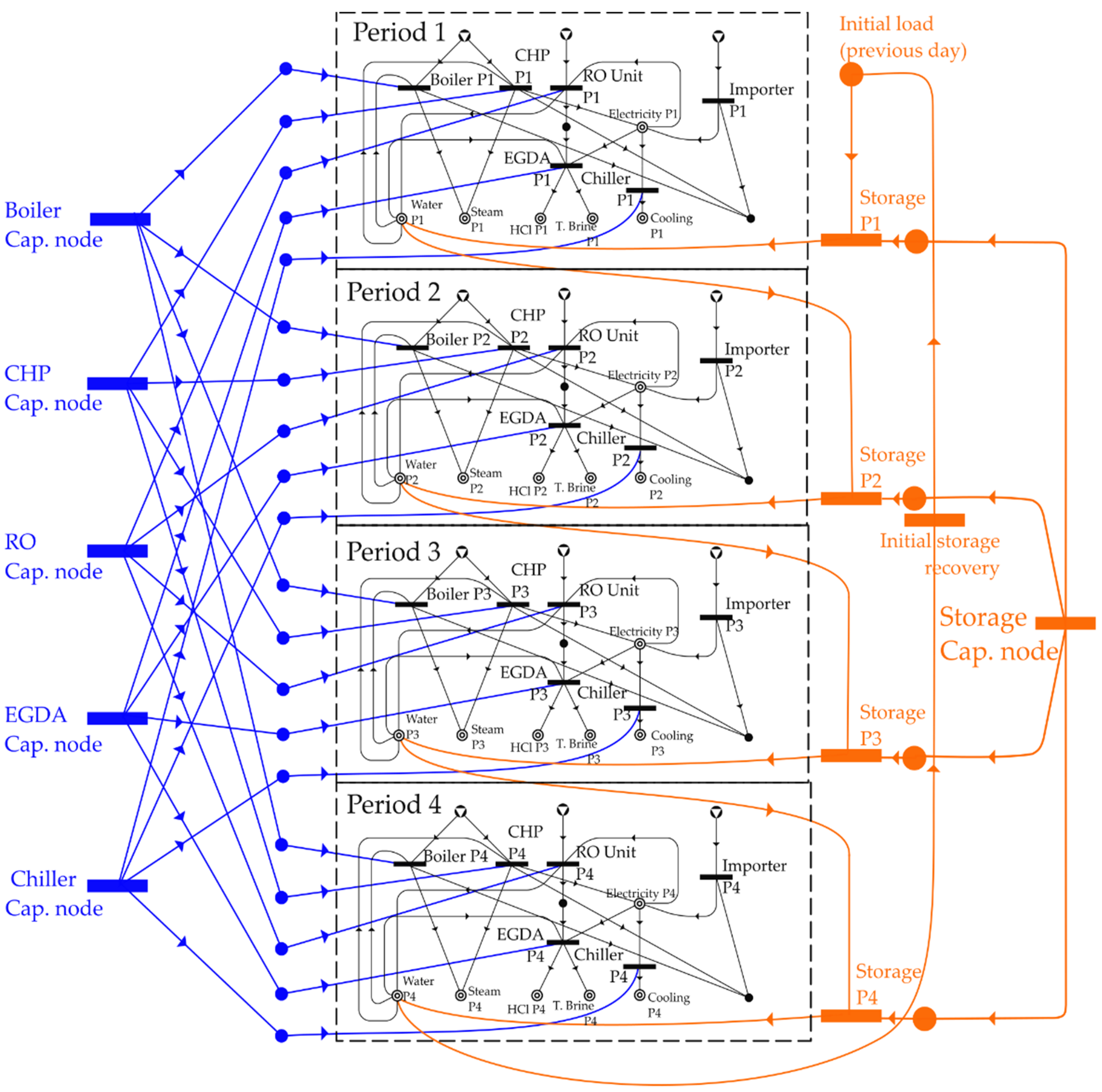
Figure 5.
Best solution in terms of profit for illustrative example of 4 periods.

Figure 6.
Operating state of the units for the different periods in most profitable solution with no CO2 limitation.
Figure 6.
Operating state of the units for the different periods in most profitable solution with no CO2 limitation.

Figure 7.
Operating state of solution 51 for the case with no limitation of CO2 emissions.
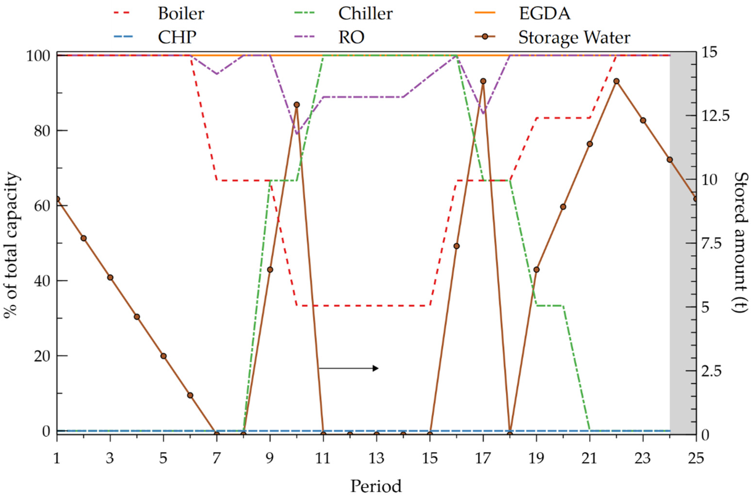
Figure 8.
The operating state of the units for the different periods in two alternative solutions with no CO2 limitation: (a) solution 6, (b) solution 66.
Figure 8.
The operating state of the units for the different periods in two alternative solutions with no CO2 limitation: (a) solution 6, (b) solution 66.

Figure 9.
Operating state of the units for the different periods in alternative with no storage units and no CO2 limitation.
Figure 9.
Operating state of the units for the different periods in alternative with no storage units and no CO2 limitation.

Figure 10.
Operating state of the units for best solution in case 2 with limit of 39,000 kg CO2 eq./day.
Figure 10.
Operating state of the units for best solution in case 2 with limit of 39,000 kg CO2 eq./day.

Figure 11.
Operating state of the units for best solution in case 3 with limit of 30,000 kg CO2 eq./day.
Figure 11.
Operating state of the units for best solution in case 3 with limit of 30,000 kg CO2 eq./day.


Table 1.
Parameters of price and demand for materials involved in the illustrative example with four periods.
Table 1.
Parameters of price and demand for materials involved in the illustrative example with four periods.
| Period Name | Electricity | Steam | Cooling | Purified Water | ||||
|---|---|---|---|---|---|---|---|---|
| Price (EUR/kwh) | Demand (kwh) | Price (EUR/kwh) | Demand (kwh) | Price (EUR/kwh) | Demand (kwh) | Price (EUR/t) | Demand (t) | |
| 1 | 0.08 | 36,000 | 0.04 | 72,000 | 0.06 | 0 | 1.2 | 600 |
| 2 | 0.12 | 60,000 | 0.04 | 48,000 | 0.06 | 3000 | 1.2 | 600 |
| 3 | 0.09 | 48,000 | 0.04 | 24,000 | 0.06 | 6000 | 1.2 | 600 |
| 4 | 0.04 | 24,000 | 0.04 | 48,000 | 0.06 | 9000 | 1.2 | 600 |
Maximum amount of HCl that can be produced is 8 t/h; price of treated brine is assumed to be 0.73 EUR/t equivalent as a carbon tax; price of biomass is 0.2 EUR/t.
Table 2.
Mass and energy balance and parameters of cost for the operating units considered for synthesis of polygeneration plant.
Table 2.
Mass and energy balance and parameters of cost for the operating units considered for synthesis of polygeneration plant.
| Materials/Operations | Boiler | CHP Unit | Chiller | RO Unit | EGDA | Importer |
|---|---|---|---|---|---|---|
| Biomass fuel (t/h) | −0.25 | −0.8 | ||||
| Imported electricity (kWe) * | −1 | |||||
| Electricity (kWe) * | 1 | −0.2 | −3 | −0.013 | 1 | |
| Steam (kWh) * | 1 | 1.6 | ||||
| Cooling (kWc) * | 1 | |||||
| Purified water (t/h) | −0.002 | −0.003 | 1 | −0.1 | ||
| HCl (t/h) | 0.1 | |||||
| Seawater (t/h) | −2 | |||||
| Brine (t/h) | 1 | −1 | ||||
| Treated brine (t/h) | 1 | |||||
| CO2 emissions (kg eq./kWh) | 0.0168 | 0.038 | 0.2 | |||
| Fixed investment cost | 45,000 | 380,000 | 44,000 | 0 | 0 | 0 |
| Proportional investment cost | 175 | 950 | 268 | 15,000 | 350 | 0 |
* The subscripts of kW are employed to differentiate between the energy in the form of electricity (e), heat (h) and cooling (c).
Table 3.
Parameters of cost and maximum capacities for storage units.
| Stored Material | Fixed Investment Cost (EUR) | Proportional Investment Cost (EUR/t) | Maximum Storage |
|---|---|---|---|
| Purified Water | 16,000 | 150 | - |
| HCl | 40,000 | 375 | 25 t |
Table 4.
Parameters of price and demand for materials involved in case study of 24 periods.
| Period | Electricity | Steam | Cooling | Purified Water | ||||
|---|---|---|---|---|---|---|---|---|
| Price (EUR/kWh) | Demand (kWh) | Price (EUR/kWh) | Demand (kWh) | Price (EUR/kWh) | Demand (kWh) | Price (EUR/t) | Demand (t) | |
| 1 | 0.05 | 4000 | 0.04 | 12,000 | 0.06 | 0 | 1.2 | 100 |
| 2 | 0.03 | 4000 | 0.04 | 12,000 | 0.06 | 0 | 1.2 | 100 |
| 3 | 0.02 | 4000 | 0.04 | 12,000 | 0.06 | 0 | 1.2 | 100 |
| 4 | 0.04 | 4000 | 0.04 | 12,000 | 0.06 | 0 | 1.2 | 100 |
| 5 | 0.05 | 6000 | 0.04 | 12,000 | 0.06 | 0 | 1.2 | 100 |
| 6 | 0.05 | 6000 | 0.04 | 12,000 | 0.06 | 0 | 1.2 | 100 |
| 7 | 0.08 | 6000 | 0.04 | 8000 | 0.06 | 0 | 1.2 | 100 |
| 8 | 0.08 | 8000 | 0.04 | 8000 | 0.06 | 0 | 1.2 | 100 |
| 9 | 0.10 | 8000 | 0.04 | 8000 | 0.06 | 1000 | 1.2 | 100 |
| 10 | 0.12 | 10,000 | 0.04 | 4000 | 0.06 | 1000 | 1.2 | 100 |
| 11 | 0.12 | 10,000 | 0.04 | 4000 | 0.06 | 1500 | 1.2 | 100 |
| 12 | 0.10 | 10,000 | 0.04 | 4000 | 0.06 | 1500 | 1.2 | 100 |
| 13 | 0.09 | 10,000 | 0.04 | 4000 | 0.06 | 1500 | 1.2 | 100 |
| 14 | 0.07 | 8000 | 0.04 | 4000 | 0.06 | 1500 | 1.2 | 100 |
| 15 | 0.07 | 8000 | 0.04 | 4000 | 0.06 | 1500 | 1.2 | 100 |
| 16 | 0.06 | 8000 | 0.04 | 8000 | 0.06 | 1500 | 1.2 | 100 |
| 17 | 0.08 | 8000 | 0.04 | 8000 | 0.06 | 1000 | 1.2 | 100 |
| 18 | 0.08 | 8000 | 0.04 | 8000 | 0.06 | 1000 | 1.2 | 100 |
| 19 | 0.09 | 10,000 | 0.04 | 10,000 | 0.06 | 500 | 1.2 | 100 |
| 20 | 0.10 | 10,000 | 0.04 | 10,000 | 0.06 | 500 | 1.2 | 100 |
| 21 | 0.11 | 10,000 | 0.04 | 10,000 | 0.06 | 0 | 1.2 | 100 |
| 22 | 0.08 | 4000 | 0.04 | 12,000 | 0.06 | 0 | 1.2 | 100 |
| 23 | 0.07 | 4000 | 0.04 | 12,000 | 0.06 | 0 | 1.2 | 100 |
| 24 | 0.06 | 4000 | 0.04 | 12,000 | 0.06 | 0 | 1.2 | 100 |
Table 5.
Best solutions in terms of profit for 5 selected cases of maximum CO2 emission.
| Characteristic | Units | Reference Stream | Case 1 | Case 2 | Case 3 | Case 4 | Case 5 |
|---|---|---|---|---|---|---|---|
| CO2 emission | kg/day | CO2 eq. | 40,300 | 39,000 | 30,000 | 25,340 | 20,000 |
| Profit | EUR/day | 853.64 | 712.88 | 341.72 | 0.26 | −668.00 | |
| Boiler capacity | kWh | Steam | 12,000 | 12,000 | 12,000 | 12,000 | 9031.3 |
| CHP capacity | kWe | Electricity | 0 | 529.2 | 3582.7 | 5000 | 6383.9 |
| Chiller | kWc | Cooling | 1500 | 1500 | 1500 | 1500 | 1500 |
| RO unit capacity | t/h | Purified water | 125.5 | 125.45 | 125.6 | 126.16 | 127.62 |
| EGDA | t/h | Treated brine | 80 | 80 | 80 | 80 | 82 |
| Imported electricity | MWh/day | Electricity | 183.6 | 176.97 | 128.71 | 103.23 | 73.12 |
| Water storage tank | t | 66 | 66.2 | 61 | 52.4 | 34.5 |
Publisher’s Note: MDPI stays neutral with regard to jurisdictional claims in published maps and institutional affiliations. |
© 2021 by the authors. Licensee MDPI, Basel, Switzerland. This article is an open access article distributed under the terms and conditions of the Creative Commons Attribution (CC BY) license (http://creativecommons.org/licenses/by/4.0/).
Share and Cite
MDPI and ACS Style
Pimentel, J.; Orosz, Á.; Aviso, K.B.; Tan, R.R.; Friedler, F. Conceptual Design of a Negative Emissions Polygeneration Plant for Multiperiod Operations Using P-Graph. Processes 2021, 9, 233. https://doi.org/10.3390/pr9020233
AMA Style
Pimentel J, Orosz Á, Aviso KB, Tan RR, Friedler F. Conceptual Design of a Negative Emissions Polygeneration Plant for Multiperiod Operations Using P-Graph. Processes. 2021; 9(2):233. https://doi.org/10.3390/pr9020233
Chicago/Turabian StylePimentel, Jean, Ákos Orosz, Kathleen B. Aviso, Raymond R. Tan, and Ferenc Friedler. 2021. "Conceptual Design of a Negative Emissions Polygeneration Plant for Multiperiod Operations Using P-Graph" Processes 9, no. 2: 233. https://doi.org/10.3390/pr9020233
Note that from the first issue of 2016, this journal uses article numbers instead of page numbers. See further details here.