
Group Acceptance Sampling Plan Using Marshall–Olkin Kumaraswamy Exponential (MOKw-E) Distribution


1
Department of Statistics, Faculty of Science, King Abdulaziz University, Jeddah 21589, Saudi Arabia
2
Department of Mathematics, Université de Caen, LMNO, Campus II, Science 3, 14032 Caen, France
3
Department of Statistics, The Islamia University of Bahawalpur, Punjab 63100, Pakistan
*
Author to whom correspondence should be addressed.
Processes 2021, 9(6), 1066; https://doi.org/10.3390/pr9061066
Submission received: 18 May 2021
/
Revised: 10 June 2021
/
Accepted: 15 June 2021
/
Published: 18 June 2021
(This article belongs to the Special Issue Neural Networks, Fuzzy Systems and Other Computational Intelligence Techniques for Advanced Process Control)
Abstract
:The current research concerns the group acceptance sampling plan in the case where (i) the lifetime of the items follows the Marshall–Olkin Kumaraswamy exponential distribution (MOKw-E) and (ii) a large number of items, considered as a group, can be tested at the same time. When the consumer’s risk and the test terminsation period are defined, the key design parameters are extracted. The values of the operating characteristic function are determined for different quality levels. At the specified producer’s risk, the minimum ratios of the true average life to the specified average life are also calculated. The results of the present study will set the platform for future research on various nano quality level topics when the items follow different probability distributions under the Marshall–Olkin Kumaraswamy scheme. Real-world data are used to explain the technique.
1. Introduction
It is now an established fact that nanotechnology affects our daily lives like never before. Advancement in nanotechnology might never have been possible without the use of appropriate statistical methods. Ref. [1] presented a detailed review of the use of statistical methods in nanoscale applications. Wherever we rely on destructive tests for testing the quality of products, sampling is the only way out. For selecting a representative sample, traditional sampling techniques (simple random sampling, systematic sampling, etc.), and their hybrids are used. For the nano process, however, new sampling techniques have been created [1]. With a smaller sample size and good use of the sampling plan, we can obtain a more precise inference and save money on sampling. In the manufacturing area, sampling plans are employed to decide on the acceptance or rejection of the incoming or outgoing batches based on some pre-specified quality, which is commonly known as lot sentencing. The size of the sample and the duration of the experiment are the two most critical factors for design engineers to consider, and both must be optimized. Acceptance sampling plans can help to achieve this optimization. Simple acceptance plans give us the minimum sample size to be used for testing. In this case, it is presumed that a single item is evaluated in a tester at a time, in order to maximize both cost and time. Ref. [2] posited the use of group to cut back on the amount of time and money invested on research. When more than one item is checked in a tester, the set of items is considered a group, justifying the name Group Acceptance Sampling Plan (GASP). As GASP is combined with truncated life testing, the result is known as a GASP based on truncated life test, which assumes that a product’s lifespan matches a certain probability distribution. The attributes group acceptance sampling plan was originally established by [3] for the truncated life test, assuming that the lifetime of each item followed the Weibull distribution. For the given values of producer and consumer risks, the number of groups and acceptance numbers are obtained simultaneously in such a sampling plan.
When the product followed various forms of probability distributions, some authors worked on a GASP based on a truncated life test. For instance, ref. [3] considered the inverse Rayleigh and log-logistic distributions, ref. [4] the extended Lomax distribution, ref. [5] the Marshall–Olkin (MO) extended Weibull distribution, ref. [6] the generalized exponential distribution and finally, and [7] the odd generalized exponential log-logistic distribution.
Since 1997, there has been a surge of interest in designing new distributions based on baseline distributions and composite approaches, with the prospect of incorporating new parameters. Indeed, the inclusion of parameters has proven to be helpful in terms of exploring skewness and tail properties, as well as enhancing the goodness-of-fit of the created family. For an exhaustive list of references on extended family of probability distributions, see [7]. Additionally, ref. [8] offered a detailed explanation of how new families of univariate continuous distributions are formed by using additional parameters. The most relevant source for the present study’s theoretical foundation is [9], where the authors developed the Kumaraswamy MO (KwMO) family of distributions, by using the MO [10] and the cumulative distribution function (cdf) as a baseline distribution in the Kumaraswamy-G family by [11], and studied its many properties. The second most relevant study is [12], which developed the MO Kumaraswamy-G (MOKw-G) family of distributions. It was based on the Kumaraswamy-G family cdf as the baseline distribution in the MO extended family, and studied its various properties at length. The primary goal of this paper is to further improve the GASPs for the MO Kumaraswamy exponential distribution (MOKw-E). As sketched in [12], the basic interests of considering the MOKw-E in this context are as follows: (i) the MOKw-E extends the modeling capabilities of the exponential distribution, and some of its powerful exponentiated versions, via a simple ratio scheme with several strategically well placed tuning parameters, (ii) the MOKw-E has a strong physical interpretation in terms of order statistics; it corresponds to the distribution of the time to the first failure of a component in a series system with N independent components, where N can be modeled by a random variable following a geometric distribution and the lifetime of a component that can be modeled by a random variable with the Kumaraswamy exponential distribution (Kw-E), (iii) thanks to the MO scheme, the MOKw-E directly benefits from strong stochastic ordering properties, and (iv) diverse sub-distributions of the MOKw-E have been proved to be particularly efficient to analyze lifetime data of various kinds (see [13,14]). As a result, we suggest that the MOKwE is an ideal candidate distribution for GASP.
For the current study, the median is taken as the quality parameter. We can refer to [15], which states that the median is a better-quality parameter for a skewed distribution than the mean. Since the MOKw-E is a skewed distribution, percentile point shall be employed as the quality parameter. Hence, the main purpose of the present study is to offer a GASP based on truncated life test assuming that the lifetimes of a product follow the MOKw-E developed by [12] with known shape parameters. Scrolling through the literature, the authors were not able to find GASP in the context of the MOKw-E. The GASP for the MOKw-E is constructed, satisfying specific consumer’s and producer’s risks at some specific quality level. Furthermore, the minimum number of groups and approval number needed for a given customer risk and test termination time are calculated for a given group size. The results of the present study will set a platform for future research based on the proposed sampling plan for studying nano quality level (NQL) when products follow different probability distributions under the MO Kumaraswamy family scheme.
Format of the Paper
The remainder of this paper is structured as follows. In Section 2, we establish the theoretical background of MOKw-G and how the probability distribution function (pdf), cdf, and quantile function of MOKw-E are worked out. Section 3 addresses the design of GASP for the lifetime percentiles under a truncated life test. Section 4 provides a summary of the proposed approach as well as real-world data examples. Finally, Section 5 summarizes the observations and addresses several possible future consequences.
2. Marshall–Olkin Kumaraswamy Exponential (MOkw-E) Distribution
First, let us recall the pdf, cdf, and quantile function of MOKw-G from which the pdf, cdf, and quantile function of MOKw-E are derived. For in-depth mathematical derivations, see [12]. The pdf MOKw-G is listed by:
where a and b constitute shape parameters with a, b > 0, α is the tilt parameter for the extended family of distributions with “”, , and is the cdf of a baseline distribution with pdf Then, the cdf of MOKw-G is given by:
and the pth quantile function tp of MOKw-G is taken form [12] as:
Using the exponential distribution as a baseline, the pdf, cdf, and the quantile function for MOKw-E can be worked out by substituting the pdf, cdf, and the quantile function of the exponential distribution in Equations (1)–(3). That is, we consider , and , . Thus, the pdf of MOKw-E is given by:
and the cdf of MOKw-E is given by:
Since the pth quantile of the exponential distribution is obtained as , the pth quantile function tp of MOKw-E using Equation (3) is:
3. Description of the Gasp
The design parameters of a GASP are now obtained in the context of MOKw-E. The steps for implementing the group acceptance plan and obtaining the design parameters were followed from [3,16], and consist of:
- Selecting ‘g’ number of groups, and allocating predefining r items to each group. Thus, the sample size for a lot is obtained as ‘n’ = g × r.
- Selecting ‘c’ with reference to the acceptance number for a group with experiment time t0.
- Simultaneously performing the experiment for ‘g’ groups and recording the number of failures for each group.
- Accepting the lot if no more than ‘c’ failures occur in all groups.
- Truncating the experiment and refusing the lot if more than ‘c’ failures occur in any group.
Thus, the proposed GASP is defined by two design parameters (g, c) for a given r. From Equation (5), it can be seen that the cdf of MOKw-E depends on and the median life of MOKw−E is given by Equation (6). It would be appropriate to calculate the termination time t0 as t0 = , where denotes a certain constant and refers to the specified life. For instance, if = 0.5, the experiment time is half that of the specified life, or, if = 3, the experiment time is three times that of the specified life. In this setting, the probability of accepting a lot is:
where ‘p’ refers to the probability that an item in a group fails before t0, and this probability of failure is derived by inserting Equation (6) in Equation (5).
Based on Equation (6), we set
Now, substituting and in Equation (5), the probability of failure is given by:
which can be expressed as:
For chosen a and b, p can be determined when and r2 are specified. The ratio of a product’s mean lifetime to the specified lifetime can be used to express the product’s quality level.
All that is required now is to minimize ASN = n = g × r, subject to the following constraints:
and
where and denote the means ratio at the consumer’s risk and at the producer’s risk, respectively. Here, and α should not be confused; as stated earlier, α is the tilt parameter for the extended family of distributions. The probabilities of failure to be used in Equations (8) and (9) are as follows:
and
Both Equations (10) and (11) above are extracted from Equation (9).
4. Discussion and Example
4.1. Discussion
The design parameters under GASP for different values of the α (1.25 and 1.50) are presented in Table 1 and Table 2. The code in R is provided in Appendix A. The values of r = 5 and 10 are considered. Then, it is noticed that a reduction in consumer’s risk, β, leads to a rise in the number of groups. Furthermore, as r2 increases, the number of groups rapidly decreases. However, after a certain point, even though the number of groups and acceptance numbers remain constant, the probability of accepting a lot begins to rise. The table also shows the impact of a1. As an example, observe that, with β = 0.25, a1 = 0.5, r2 = 6, α = 1.25, and, for r = 5, a total of eight groups, i.e., 8 × 5 = 40 number of units, are necessary on the life test. Additionally, when r = 10, then only two groups, i.e., 2 × 5 = 10 number of units, are necessary for the life test. As a result, in this case, 10 groups would be preferable. Table 2 reports α = 1.50. According to the reported values, increasing the shape parameter value results in a smaller group size for the associated plan. For the considered GASP, under the MOKw-E and using median lifetime as the quality parameter, the number of groups decreases and the OC values (P(a)) increase when the true median life increases. This is presented in Table 1 for various values of the parameters (α = 1.25, β = 0.01, r = 10, and a1 = 1.0)
| m/m0 = r2 | 4 | 6 | 8 |
| G | 11 | 6 | 3 |
| C | 5 | 4 | 3 |
| P(a) | 0.9653 | 0.9758 | 0.9793 |
To cross check the results shown in Table 1 and Table 2, an example from [17] is considered. Suppose that the lifetime of ball bearings placed on a test follow MOKw-E, with the shape parameter α = 1.25, and the mean specified life of the ball bearings is 2000 cycles. When the true mean life is 2000 cycles, the consumer faces a 25% risk, while the producer faces a 5% risk when the true mean life is 4000 cycles. Now, an experimenter wants to run a 1000-cycle experiment with 10 units in each group to see if the ball bearings’ mean life is longer than the specified life. In this context, we have α = 1.50, = 2000 cycles, a1 = 0.5, r = 10, β = 0.25, r1 = 1, producer’s risk = 0.05, and r2 = 4. In addition, from Table 2, we have g = 39 and c = 3. This implies that 195 units (n = g × r) must be drawn, with five units assigned to each of the 39 groups. If no more than three units fail in each of these groups before 1000 cycles, the mean life of the ball bearings will be statistically assured to be greater than the specified life. If a quality control engineer wants to test the hypothesis that ball bearings have a life span of 4000 cycles but a true average life of four times that, he or she can test 39 groups of five units each; if fewer than three units fail in 1000 cycles; as a1 = 0.5 and the mean life length is in thousands of cycles, the engineer will infer that the life is more than 4000 cycles with 95 percent confidence. Therefore, the lot under investigation should be accepted.
4.2. Example
We consider now a data set which consists of a sample of 50 observed values of breaking stress of carbon fibers given by [18]. The unit is Gba. The data set can be expanded as follows: {1.12,0.17,0.64,4.32,1.22,0.37,1.16,1.42,0.09,1.67,0.13,0.25,0.08,0.04,2.35,0.20,0.78,0.34,1.02,0.17,1.76,2.39,0.50,1.35,3.36,0.45,0.90,2.92,6.53,1.62,7.46,3.19,2.49,1.40,7.49,0.57,0.14,0.63,5.23,0.71,0.68,0.12,0.09,3.47,5.93,1.82,4.20,7.29,3.13,3.41}.
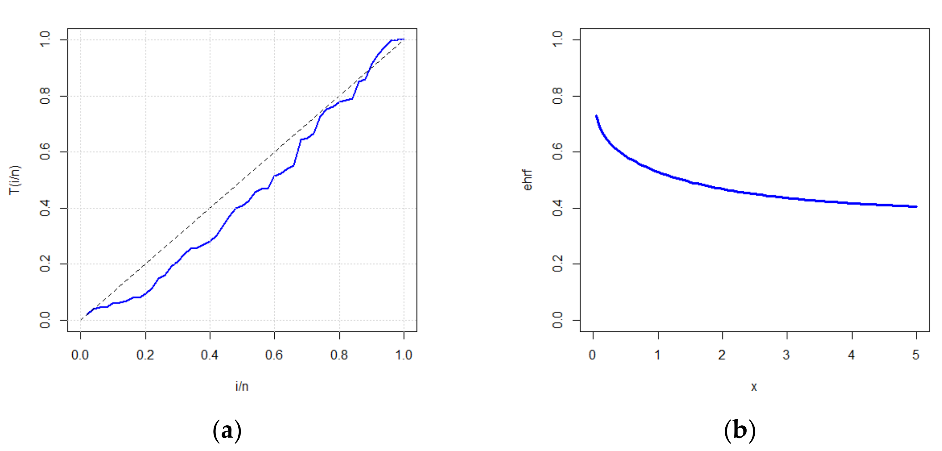
The maximum likelihood estimates with standard errors (in parentheses) of the four parameters of MOKw−E for the data are 0.2978 (0.5117), 0.9356 (0.2371), 1.2805 (0.6596), and 0.6361 (0.5377). The ‘maximum distance’ between the data and the fitted MOKw−E is 0.0681 with a p-value of 0.9743, according to the Kolmogorov–Smirnov (K–S) test. Figure 1 depicts the histogram of the data with the estimated pdf, the empirical cdf with the estimated cdf, the probability–probability (P–P) plot, and the quantile–quantile (Q–Q) plot. Figure 2 completes Figure 1 by considering the total time on test (TTT) plot to have some information regarding the underlying hazard rate function (hrf) and the estimated hazard rate function.
Figure 1 shows that MOKw-E has a good fit for the carbon fibers data set, whereas Figure 2 displays the total time on test (TTT) plot and the estimated hrf that the given data set has a decreasing hazard rate. Thus, MOKw-E provides a reasonable fit of the data. The plan parameters for the 50th percentile are also calculated using fitted parametric values and are shown in Table 3. The behavior of the plan parameters in Table 3 matches the values of the plan parameters in Table 1 and Table 2.
5. Conclusions
This study emphasizes a GASP assuming that the lifetime of the product follows MOKw-E. All the attention is focused on certain key plan parametric quantities. The number of categories, ‘g’, and the acceptance number, ‘c’, are calculated by balancing the risks of the manufacturer and the customer. For all the parametric combinations considered in this paper, it is observed in the proposed plan that as the percentile ratio increases, g decreases, and as the number of items in each group increases, the number of groups decreases, which is consistent with the results given in [7].
Author Contributions
Conceptualization, A.M.A., K.K., C.C. and F.J.; methodology, A.M.A., K.K., C.C. and F.J.; validation, A.M.A., K.K., C.C. and F.J.; formal analysis, A.M.A., K.K., C.C. and F.J.; investigation, A.M.A., K.K., C.C. and F.J.; writing—original draft preparation, A.M.A., K.K., C.C and F.J.; writing—review and editing, A.M.A., K.K., C.C. and F.J. All authors have read and agreed to the published version of the manuscript.
Funding
This research received no external funding.
Informed Consent Statement
Not applicable.
Data Availability Statement
The data are fully available in the article or the mentioned references.
Acknowledgments
The authors wish to express their gratitude to the Department of Statistics, King Abdulaziz University for providing the wherewithal coupled with the conducive research environment for carrying out the present study. Moreover, the authors would also like to extend thanks to all the authors whose work has been cited herein for providing the requisite stimulus for research on the current topic.
Conflicts of Interest
There exists no conflict of interest amongst the authors regarding the contents and publication of this research article.
Appendix A
R code for the considered sampling plan.
g=sEquation(1,1000,1);c=c(0,1,2,3,4,5);lp2=double(length(g));
lp1=double(length(g));lp21=double(length(c)); lp22=double(length(c));
lp23=double(length(c));lp24=double(length(c));G1=double(length(c));
G2=double(length(c));G3=double(length(c));G4=double(length(c));
p=function(alp,p,ratio,a,b ){
  nu=log(1-(((1-(1-((alp*p)/(1-(1-alp)*p)))^(1/b)))^(1/a)))
  d=(1-((1-exp(nu*((ratio)^-1)*a1))^a))
  y=(((1-d)^b)/(1-((1-alp)*(1-d)^b)));return(y)
}
p2=round(p(2,0.5,c(2,4,6,8,10),1,1,0.5),4);
p2; p1=round(p(2,0.5,1,1,1,0.5),4);p1
for(i in 1:length(c)){
  for(j in 1:length(g)){
    lp2[j]=(pbinom(c[i],10,p2[2]))^j
    lp1[j]=(pbinom(c[i],10,p1))^j
}
  G1[i]=min(which(lp2>=0.95 & lp1<0.25));lp21[i]=round(lp2[G1[i]],4);
  G2[i]=min(which(lp2>=0.95 & lp1<0.10));lp22[i]=round(lp2[G2[i]],4);
  G3[i]=min(which(lp2>=0.95 & lp1<0.05));lp23[i]=round(lp2[G3[i]],4);
  G4[i]=min(which(lp2>=0.95 & lp1<0.01));lp24[i]=round(lp2[G4[i]],4);
}
cbind(c,G1,lp21,G2,lp22,G3,lp23,G4,lp24).
|
References
- Lu, J.C.; Jeng, S.L.; Wang, K. A review of statistical methods for quality improvement and control in nanotechnology. J. Qual. Technol. 2009, 41, 148–164. [Google Scholar] [CrossRef]
- Jun, C.H.; Balamurali, S.; Lee, S.H. Variables sampling plans for Weibull distributed lifetimes under sudden death testing. IEEE Trans. Reliab. 2006, 55, 53–58. [Google Scholar] [CrossRef]
- Aslam, M.; Jun, C.H. A Group Acceptance Sampling Plans for Truncated Life Tests based on The Inverse Rayleigh And Log-Logistic Distributions. Pak. J. Stat. 2009, 25, 107–119. [Google Scholar]
- Rao, G.S. A group acceptance sampling plans based on truncated life tests for Marshall-Olkin extended Lomax distribution. Electron. J. Appl. Stat. Anal. 2009, 3, 18–27. [Google Scholar]
- Rao, G.S. A group acceptance sampling plans for lifetimes following a Marshall–Olkin extended Weibull distribution. Stat. Appl. 2010, 8, 135–144. [Google Scholar]
- Aslam, M.; Kundu, D.; Jun, C.H.; Ahmad, M. Time truncated group acceptance sampling plans for generalized exponential distribution. J. Test. Eval. 2011, 39, 671–677. [Google Scholar]
- Sivakumar, D.C.U.; Kanaparthi, R.; Rao, G.S.; Kalyani, K. The Odd generalized exponential log-logistic distribution group acceptance sampling plan. Stat. Transit. New Ser. 2019, 20, 103–116. [Google Scholar] [CrossRef] [Green Version]
- Tahir, M.H.; Nadarajah, S. Parameter induction in continuous univariate distributions: Well-established G families. An. Acad. Bras. Ciências 2015, 87, 539–568. [Google Scholar] [CrossRef] [PubMed]
- Alizadeh, M.; Tahir, M.H.; Cordeiro, G.M.; Zubair, M.; Hamedani, G.G. The Kumaraswamy Marshal-Olkin family of distributions. J. Egypt. Math. Soc. 2015, 23, 546–557. [Google Scholar] [CrossRef] [Green Version]
- Marshall, A.W.; Olkin, I. A new method for adding a parameter to a family of distributions with application to the exponential and Weibull families. Biometrika 1997, 84, 641–652. [Google Scholar] [CrossRef]
- Cordeiro, G.M.; de Castro, M. A new family of generalized distributions. J. Stat. Comput. Simul. 2011, 81, 883–898. [Google Scholar] [CrossRef]
- Handique, L.; Chakraborty, S. The Marshall-Olkin-Kumaraswamy-G family of distributions. arXiv 2015, arXiv:1509.08108. [Google Scholar] [CrossRef] [Green Version]
- Ghitany, M.E.; Al-Hussaini, E.K.; Al-Jarallah, R.A. Marshall–Olkin extended Weibull distribution and its application to censored data. J. Appl. Stat. 2005, 32, 1025–1034. [Google Scholar] [CrossRef]
- Ristić, M.M.; Kundu, D. Marshall-Olkin generalized exponential distribution. Metron 2015, 73, 317–333. [Google Scholar] [CrossRef]
- Gupta, S.S. Life test sampling plans for normal and lognormal distributions. Technometrics 1962, 4, 151–175. [Google Scholar] [CrossRef]
- Khan, K.; Alqarni, A. A group acceptance sampling plan using mean lifetime as a quality parameter for inverse Weibull distribution. Adv. Appl. Stat. 2020, 649, 237–249. [Google Scholar] [CrossRef]
- Singh, S.; Tripathi, Y.M. Acceptance sampling plans for inverse Weibull distribution based on truncated life test. Life Cycle Reliab. Saf. Eng. 2017, 6, 169–178. [Google Scholar] [CrossRef] [Green Version]
- Nichols, M.D.; Padgett, W.J. A bootstrap control chart for Weibull percentiles. Qual. Reliab. Eng. Int. 2006, 22, 141–151. [Google Scholar] [CrossRef]
Figure 1.
Examples of fits of MOKw-E for the carbon fibers dataset: (a) histogram fitted by the estimated pdf, (b) empirical cdf fitted by the estimated cdf, (c) P–P plot, and (d) Q–Q plot.
Figure 1.
Examples of fits of MOKw-E for the carbon fibers dataset: (a) histogram fitted by the estimated pdf, (b) empirical cdf fitted by the estimated cdf, (c) P–P plot, and (d) Q–Q plot.
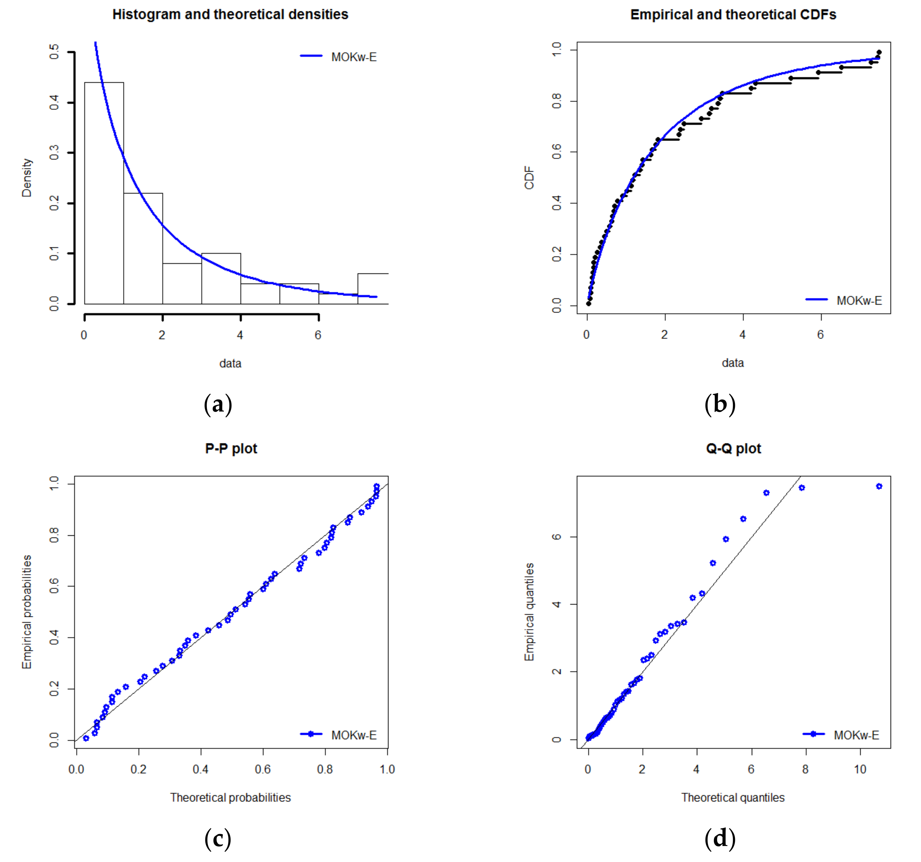
Figure 2.
Plot of (a) TTT, and (b) the estimated hrf (ehrf) for the carbon fibers data set.

Table 1.
GASP for a = 1, b = 1, and α = 1.25, showing minimum g and c.
| β | r2 | r = 5 | r = 10 | ||||||||||
|---|---|---|---|---|---|---|---|---|---|---|---|---|---|
| a1 = 0.5 | a1 = 1 | a1 = 0.5 | a1 = 1 | ||||||||||
| g | c | P(a) | g | c | P(a) | g | c | P(a) | g | c | P(a) | ||
| 0.25 | 2 | - | - | - | - | - | - | - | - | - | - | - | - |
| 4 | 41 | 3 | 0.9852 | 8 | 3 | 0.9678 | 3 | 3 | 0.9693 | 2 | 4 | 0.9620 | |
| 6 | 8 | 2 | 0.9809 | 3 | 2 | 0.9552 | 2 | 2 | 0.9552 | 1 | 3 | 0.9743 | |
| 8 | 8 | 2 | 0.9914 | 3 | 2 | 0.9786 | 2 | 2 | 0.9972 | 1 | 3 | 0.9897 | |
| 0.10 | 2 | - | - | - | - | - | - | - | - | - | - | - | - |
| 4 | 67 | 3 | 0.9760 | 83 | 4 | 0.9863 | 13 | 4 | 0.9840 | 6 | 5 | 0.9809 | |
| 6 | 13 | 2 | 0.9691 | 13 | 3 | 0.9869 | 5 | 3 | 0.9870 | 3 | 4 | 0.9878 | |
| 8 | 13 | 2 | 0.9861 | 4 | 2 | 0.9715 | 3 | 2 | 0.9681 | 2 | 3 | 0.9794 | |
| 0.05 | 2 | - | - | - | - | - | - | - | - | - | - | - | - |
| 4 | 88 | 3 | 0.9686 | 107 | 4 | 0.9823 | 17 | 4 | 0.9792 | 8 | 5 | 0.9746 | |
| 6 | 16 | 2 | 0.9621 | 16 | 3 | 0.9839 | 7 | 3 | 0.9818 | 4 | 4 | 0.9838 | |
| 8 | 16 | 2 | 0.9829 | 5 | 2 | 0.9645 | 3 | 2 | 0.9681 | 2 | 3 | 0.9794 | |
| 0.01 | 2 | - | - | - | - | - | - | - | - | - | - | - | - |
| 4 | 134 | 3 | 0.9526 | 165 | 4 | 0.9729 | 26 | 4 | 0.9683 | 11 | 5 | 0.9653 | |
| 6 | 134 | 3 | 0.9892 | 25 | 3 | 0.9749 | 10 | 3 | 0.9741 | 6 | 4 | 0.9758 | |
| 8 | 25 | 2 | 0.9734 | 25 | 3 | 0.9910 | 10 | 3 | 0.9907 | 3 | 3 | 0.9793 | |
Remark: The cells with hyphens (-) indicate that a very large sample size is needed.
Table 2.
GASP for a = 1, b = 1, and α = 1.50, showing minimum g and c.
| β | r2 | r = 5 | r = 10 | ||||||||||
|---|---|---|---|---|---|---|---|---|---|---|---|---|---|
| a1 = 0.5 | a1 = 1 | a1 = 0.5 | a1 = 1 | ||||||||||
| g | c | P(a) | g | c | P(a) | g | c | P(a) | g | c | P(a) | ||
| 0.25 | 2 | - | - | - | - | - | - | - | - | - | - | - | - |
| 4 | 39 | 3 | 0.9803 | 9 | 3 | 0.9553 | 3 | 3 | 0.9853 | 5 | 5 | 0.9786 | |
| 6 | 8 | 2 | 0.9747 | 9 | 3 | 0.9877 | 3 | 3 | 0.9888 | 1 | 3 | 0.9668 | |
| 8 | 8 | 2 | 0.9886 | 9 | 3 | 0.9726 | 2 | 2 | 0.9716 | 1 | 3 | 0.9860 | |
| 0.10 | 2 | - | - | - | - | - | - | - | - | - | - | - | - |
| 4 | 65 | 3 | 0.9674 | 109 | 4 | 0.9762 | 13 | 4 | 0.9763 | 7 | 5 | 0.9701 | |
| 6 | 12 | 2 | 0.9623 | 15 | 3 | 0.9797 | 5 | 3 | 0.9814 | 4 | 4 | 0.9773 | |
| 8 | 12 | 2 | 0.9826 | 5 | 3 | 0.9547 | 3 | 2 | 0.9576 | 2 | 3 | 0.9721 | |
| 0.05 | 2 | - | - | - | - | - | - | - | - | - | - | - | - |
| 4 | 85 | 3 | 0.9575 | 142 | 4 | 0.9691 | 17 | 4 | 0.9691 | 9 | 5 | 0.9617 | |
| 6 | 16 | 2 | 0.9501 | 20 | 3 | 0.9730 | 7 | 3 | 0.9741 | 5 | 4 | 0.9717 | |
| 8 | 16 | 2 | 0.9768 | 20 | 3 | 0.9898 | 3 | 2 | 0.9576 | 3 | 3 | 0.9585 | |
| 0.01 | 2 | - | - | - | - | - | - | - | - | - | - | - | - |
| 4 | 132 | 3 | 0.9876 | 218 | 4 | 0.9530 | 25 | 4 | 0.9549 | 10 | 5 | 0.9607 | |
| 6 | 125 | 3 | 0.9846 | 30 | 3 | 0.9597 | 10 | 3 | 0.9632 | 7 | 4 | 0.9606 | |
| 8 | 24 | 2 | 0.9654 | 30 | 3 | 0.9848 | 10 | 3 | 0.9862 | 5 | 3 | 0.9872 | |
Table 3.
GASP for MLE , , and , showing minimum g and c.
| β | r2 | r = 5 | r = 10 | ||||||||||
|---|---|---|---|---|---|---|---|---|---|---|---|---|---|
| a1 = 0.5 | a1 = 1 | a1 = 0.5 | a1 = 1 | ||||||||||
| g | c | P(a) | g | c | P(a) | g | c | P(a) | g | c | P(a) | ||
| 0.25 | 2 | - | - | - | - | - | - | - | - | - | 17 | 5 | 9575 |
| 4 | 33 | 2 | 0.9785 | 6 | 2 | 0.9715 | 6 | 2 | 0.9650 | 3 | 3 | 0.9813 | |
| 6 | 7 | 1 | 0.9576 | 6 | 2 | 0.9917 | 6 | 2 | 0.9896 | 2 | 2 | 0.9728 | |
| 8 | 7 | 1 | 0.9764 | 2 | 1 | 0.9717 | 2 | 1 | 0.9714 | 2 | 2 | 0.9882 | |
| 0.10 | 2 | - | - | - | - | - | - | - | - | - | - | - | - |
| 4 | 63 | 2 | 0.9646 | 10 | 2 | 0.9530 | 31 | 3 | 0.9873 | 4 | 3 | 0.9752 | |
| 6 | 63 | 2 | 0.9900 | 10 | 2 | 0.9861 | 9 | 2 | 0.9845 | 2 | 2 | 0.9728 | |
| 8 | 11 | 1 | 0.9632 | 3 | 1 | 0.9578 | 9 | 2 | 0.9935 | 2 | 2 | 0.9882 | |
| 0.05 | 2 | - | - | - | - | - | - | - | - | - | - | - | - |
| 4 | 81 | 2 | 0.9547 | 62 | 3 | 0.9872 | 41 | 5 | 0.9832 | 5 | 3 | 0.9691 | |
| 6 | 81 | 2 | 0.9872 | 13 | 2 | 0.9820 | 12 | 2 | 0.9793 | 3 | 2 | 0.9595 | |
| 8 | 14 | 1 | 0.9534 | 13 | 2 | 0.9926 | 12 | 2 | 0.9914 | 3 | 2 | 0.9824 | |
| 0.01 | 2 | - | - | - | - | - | - | - | - | - | - | - | - |
| 4 | 138 | 2 | 0.9635 | 94 | 3 | 0.9806 | 62 | 5 | 0.9747 | 8 | 3 | 0.9510 | |
| 6 | 125 | 2 | 0.9803 | 19 | 2 | 0.9738 | 18 | 2 | 0.9692 | 8 | 3 | 0.9896 | |
| 8 | 125 | 2 | 0.9920 | 19 | 2 | 0.9892 | 18 | 2 | 0.9871 | 4 | 2 | 0.9765 | |
Publisher’s Note: MDPI stays neutral with regard to jurisdictional claims in published maps and institutional affiliations. |
© 2021 by the authors. Licensee MDPI, Basel, Switzerland. This article is an open access article distributed under the terms and conditions of the Creative Commons Attribution (CC BY) license (https://creativecommons.org/licenses/by/4.0/).
Share and Cite
MDPI and ACS Style
Almarashi, A.M.; Khan, K.; Chesneau, C.; Jamal, F. Group Acceptance Sampling Plan Using Marshall–Olkin Kumaraswamy Exponential (MOKw-E) Distribution. Processes 2021, 9, 1066. https://doi.org/10.3390/pr9061066
AMA Style
Almarashi AM, Khan K, Chesneau C, Jamal F. Group Acceptance Sampling Plan Using Marshall–Olkin Kumaraswamy Exponential (MOKw-E) Distribution. Processes. 2021; 9(6):1066. https://doi.org/10.3390/pr9061066
Chicago/Turabian StyleAlmarashi, Abdullah M., Khushnoor Khan, Christophe Chesneau, and Farrukh Jamal. 2021. "Group Acceptance Sampling Plan Using Marshall–Olkin Kumaraswamy Exponential (MOKw-E) Distribution" Processes 9, no. 6: 1066. https://doi.org/10.3390/pr9061066
Note that from the first issue of 2016, this journal uses article numbers instead of page numbers. See further details here.