Abstract
The problem of quantifying the vulnerability of graphs has received much attention nowadays, especially in the field of computer or communication networks. In a communication network, the vulnerability measures the resistance of the network to disruption of operation after the failure of certain stations or communication links. If we think of a graph as modeling a network, the average lower 2-domination number of a graph is a measure of the graph vulnerability and it is defined by , where the lower 2-domination number, denoted by , of the graph G relative to v is the minimum cardinality of 2-domination set in G that contains the vertex v. In this paper, the average lower 2-domination number of wheels and some related networks namely gear graph, friendship graph, helm graph and sun flower graph are calculated. Then, we offer an algorithm for computing the 2-domination number and the average lower 2-domination number of any graph G.
Keywords:
graph vulnerability; connectivity; network design and communication; domination number; average lower 2-domination number MSC:
05C40; 05C69; 68M10; 68R10
1. Introduction
Graph theory has seen an explosive growth due to interaction with areas like computer science, operation research, etc. In particular, it has become one of the most powerful mathematical tools in the analysis and study of the architecture of a network. The most common networks are telecommunication networks, computer networks, road and rail networks and other logistic networks [1]. In a communication network, the measures of vulnerability are essential to guide the designers in choosing a suitable network topology. They have an impact on solving difficult optimization problems for networks [2,3].
The graph vulnerability relates to the study of a graph when some of its elements (vertices or edges) are removed. The measures of graph vulnerability are usually invariants that measure how a deletion of one or more network elements changes properties of the network [4]. In the literature, various measures have been defined to measure the robustness of a network and a variety of graph theoretic parameters have been used to derive formulas to calculate network vulnerability. The best known measure of reliability of a graph is its connectivity. The connectivity is defined to be the minimum number of vertices whose deletion results in a disconnected or trivial graph [5].
The connectivity of a graph G is denoted by and it is defined as follows:
where is the number of components of the graph .
The toughness [6], the integrity [7], the domination number [8], the bondage number [9,10], the edge eccentric connectivity number [11], etc., have been proposed for measuring the vulnerability of networks. Recently, some average vulnerability parameters like the average lower independence number [12,13], the average lower domination number [13,14,15,16,17], the average connectivity number [18], the average lower connectivity number [19] and the average lower bondage number [4] have been defined.
Let be a simple undirected graph of order n. We begin by recalling some standard definitions that we need throughout this paper. For any vertex , the open neighborhood of v is and closed neighborhood of v is . The degree of vertex v in G denoted by , that is, the size of its open neighborhood [8]. The minimum degree of graph G is denoted by . A set is a dominating set if every vertex in is adjacent to at least one vertex in S. The minimum cardinality taken over all dominating sets of G is called the domination number of G and denoted by [8]. Another domination concept is 2-domination number. A 2-dominating set of a graph G is a set of vertices of graph G such that every vertex of has at least two neighbors in D. The 2-domination number of a graph G, denoted by , is the minimum cardinality of a 2-dominating set of the graph G [8,20,21,22].
In 2004, Henning introduced the concept of average domination and average independence in [13]. Moreover, the average lower domination and average lower independence number are the theoretical vulnerability parameters for a network that modeled a graph [12,15]. The average lower domination number of a graph G, denoted by , is defined as follows:
where the lower domination number, denoted by , is the minimum cardinality of a dominating set of the graph G that contains the vertex v [13,16]. In [15], an algorithm is given for computing the average lower domination number of any graph G.
In 2015, a new graph theoretical parameter namely the average lower 2-domination number was defined in [23,24]. The average lower 2-domination number of a graph G, denoted by , is defined as follows:
where the lower 2-domination number, denoted by , is the minimum cardinality of a dominating set of the graph G that contains the vertex v [23,24].
If we think of a graph as modeling a network, then the average lower 2-domination number can be more sensitive for the vulnerability of graphs than the other known vulnerability measures of a graph [23]. We consider two connected simple graphs G and H in Figure 1, where and . Graphs G and H have not only equal the connectivity but also equal the domination number, the average lower domination number and the 2-domination number such as , , and . The results can be checked by readers. So, how can we distinguish between the graphs G and H?
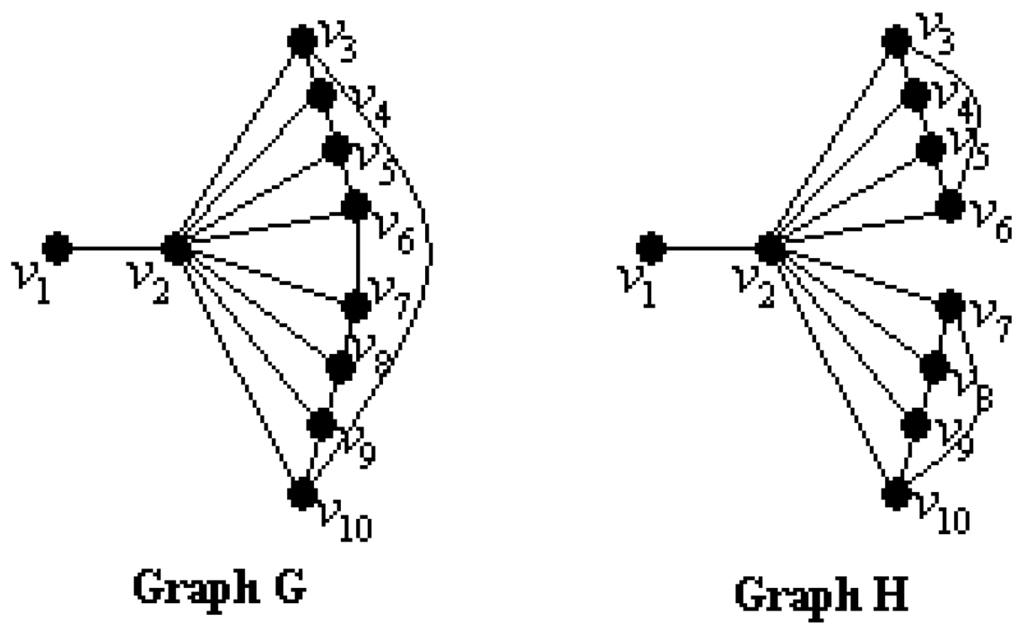
Figure 1.
Graphs G and H.
When we compute and , we get and . So, the average lower 2-domination number may be used for distinguish between these two graphs G and H. Since , we can say that the graph H is more vulnerable than the graph G. In other words, the graph G is tougher than the graph H [23,24].
The wheel graph has been used in different areas such as the wireless sensor networks, the vulnerability of networks, and so on. The wheel graph has many good properties. From the standpoint of the hub vertex, all elements, including vertices and edges, are in its one-hop neighborhood, which indicates that the wheel structure is fully included in the neighborhood graph of the hub vertex. Furthermore, wheel graphs are important for localizability because they are globally rigid in 2D space, which indicates an approach to identifying localizable vertices [25]. Moreover, the wheels and various related graphs have been studied for many reasons. The gear graphs, the friendship graph, the helm graphs and the sun flower graphs are among such graphs. The definitions of these graphs will be given in Section 3. In [26], Aytac and Odabas compute the residual closeness for wheels and related graphs. In [27], Javaid and Shokat give upper bounds for the cardinality of vertices in some wheel related graphs with a given partition dimension k.
Our aim in this paper is to study a new vulnerability parameter, called the average lower 2-domination number. In Section 2, well-known basic results are given for the average lower domination number, the average lower 2-domination number and the 2-domination number. In Section 3, we compute the average lower 2-domination numbers of wheels and some related graphs. Finally, an algorithm is proposed for computing the 2-domination number and the average lower 2-domination numbers of any given graph in Section 4.
2. Basic Results
In this section, well known basic results are given with regard to the average lower domination number, the average lower 2-domination number and the 2-domination number.
Theorem 1.
[13] Let G be any graph of order n with the domination number , then
with equality if and only if G has a unique -set.
Theorem 2.
[13] If is a star graph of order n, where , then .
Theorem 3.
[13] If is a path graph of order n, then
Theorem 4.
[13] If is a cycle graph of order n, then .
Theorem 5.
[13] If is a complete graph of order n, then .
Observation 1.
If is a wheel graph of order , then .
Theorem 6.
[28] If is a complete graph of order n, then .
Theorem 7.
[28] If is a path graph of order n, then .
Theorem 8.
[28] If is a cycle graph of order n, where , then .
Theorem 9.
[28] If is a wheel graph of order , where , then
Theorem 10.
[23] Let G be any connected graph of order n. If -set is unique, then
Theorem 11.
[23] Let G be any connected graph of order n. If , then
Theorem 12.
[23] Let G be any connected graph of order . Then, .
Theorem 13.
[23] If is a path graph of order n, then
Theorem 14.
[23] If is a cycle graph of order n, then .
Theorem 15.
[23] If is a complete graph of order n, then .
Theorem 16.
[23] If is a star graph of order n, where , then .
3. The Average Lower 2-Domination Number of Wheels Related Graphs
In this section, we have calculated the average lower 2-domination number of wheels and related graphs such as the wheel graph , the gear graph , the friendship graph , the helm graph and the sun flower graph . Now, we recall the definitions of these graphs.
Definition 1.
[26] The wheel graph with n spokes is a graph that contains an n-cycle and one additional central vertex that is adjacent to all vertices of the cycle. Wheel graph has -vertices and -edges.
Definition 2.
[12] The gear graph is a wheel graph with a vertex added between each pair adjacent graph vertices of the outer cycle. The gear graph has -vertices and -edges.
Definition 3.
[26] The friendship graph is collection of n triangles with a common vertex. The friendship graph has -vertices and -edges.
Definition 4.
[27] The helm graph is the graph obtained from an n-wheel graph by adjoining a pendant edge at each vertex of the cycle. The helm graph has -vertices and -edges.
Definition 5.
[27] The sun flower graph the graph obtained from an n-wheel graph with central vertex and n-cycle and additional n vertices where is joined by edges to for where is taken modulo n. The sun flower graph has -vertices and -edges.
We display the graphs and in Figure 2.
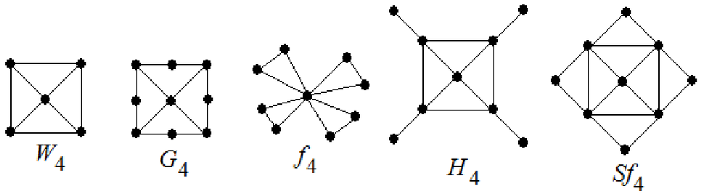
Figure 2.
Graphs and .
Theorem 17.
If is a wheel graph of order , where , then .
Proof.
The - set of a graph , , is a set with the vertex and vertices from the set . So, . Thus, is obtained for every vertex . As a result, we get .
Remark 1.
Let and be wheels graph with order 3 and 4, respectively. Then, and .
Remark 2.
If is a wheel graph of order , then .
Theorem 18.
If is a gear graph of order , then .
Proof.
We partition the vertices of graph into three subsets , and as follows:
When the is calculated for all vertices v in the graph , each vertex satisfies one of the three cases below.
Case 1.
Let be the vertex of . The center vertex is adjacent to n vertices in . Thus, all vertices of are 1-dominated. By the definition of gear graphs, the whole vertex set (or ) is taken to -set, then is obtained.
Case 2.
Let be the vertex of . Clearly every vertex of the graph is 2-dominated by the vertices of . As a result, we have , where .
Case 3.
Let be the vertex of . The -set including vertex is similar to -set in the Case 1. So, we have , where .
By Cases 1, 2 and 3, we have:
Theorem 19.
If is a friendship graph of order , then .
Proof.
By the definition of the friendship graph and 2-domination number, a -set must include the vertex whose degree is 2n. Thus, 2n-vertices are 1-dominated by the vertex . Furthermore, n-disjoint graphs are formed by these 2n-vertices in the graph . When any vertex of each graph is taken to a -set, is obtained. It is easy to see that for every vertex . Thus, we get .
Theorem 20.
If is a helm graph of order , then .
Proof.
Since the -set is unique in the graph , we have by the Theorem 10. As a result, is obtained.
Theorem 21.
If is a sun flower graph of order , then .
Proof.
The proof follows directly from the Theorem 18.
It is point out that the gear graph is tougher than the friendship graph and the helm graph , where and . Similarly, the wheel graph is tougher than the sun flower graph , where and . Readers can see that these results are shown in Figure 3 and Figure 4.
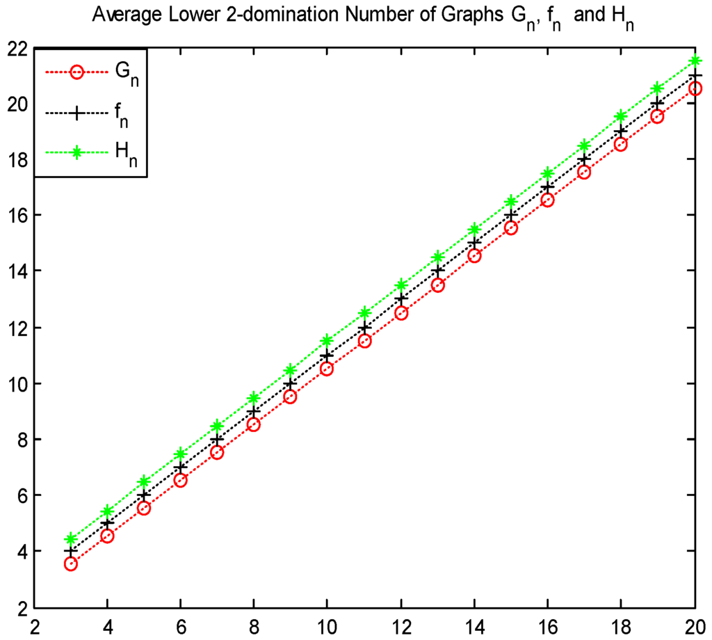
Figure 3.
Values of , and .
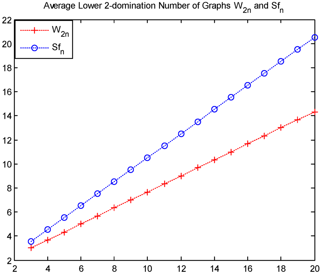
Figure 4.
Values of and .
4. An Algorithm for Computing the Average Lower 2-Domination Number
In this section, the algorithm in [29] which finds the domination number and all the minimal dominating sets of a graph is improved. The improved algorithm also computes the 2-domination number and the average lower 2-domination number of a graph. The definitions used in the algorithm below are found in [29].
positive integer
element of
array of
: real number
BEGIN
for to do
begin
;
if then end if;
if then
ELSE
for to do
begin
for to do
begin
if and and and
then end if;
end; {for k}
end; {for i}
end if;
end; {for j}
for to do
begin
;
end;
;
;
for do
;
;
for to do
begin
;
for to do
begin
if then end if;
if then end if;
if then end if;
end; {for j}
;
end; {for i}
;
END.
Example 1.
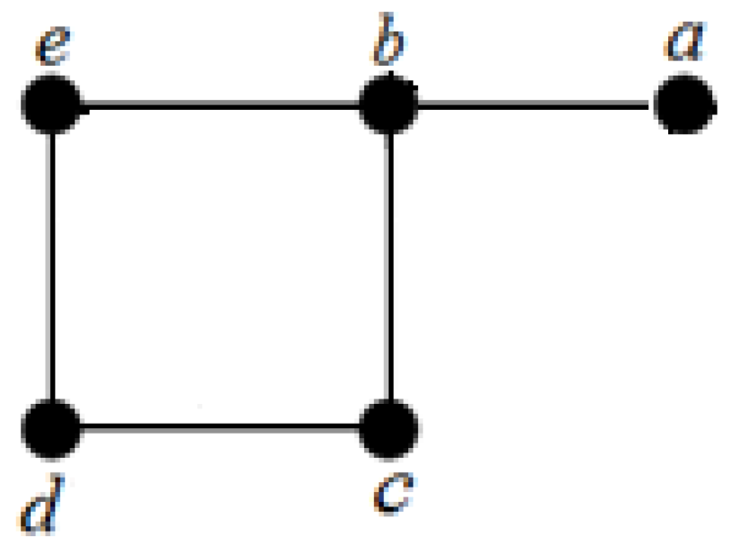
Compute the 2-domination number and the average lower 2-domination number of graph G in Figure 5.
Figure 5.
Graph G with 5-vertices and 5-edges.
Firstly, we must find function f as follows:
Then, two mathematical logic functions are used as follows:
Thus, we have
Furthermore, we have .
Clearly, the 2-domination sets and have been found by the algorithm. Thus, we get .
5. Conclusions
Communication systems are often subjected to failures and attacks. A variety of measures have been proposed in the literature to quantify the robustness of networks and a number of graph theoretic parameters have been used to derive formulas for calculating network reliability. In this paper we have studied the average lower 2-domination number for graph vulnerability. The average lower 2-domination number can be more sensitive than the other measures of vulnerability like connectivity, domination number, average lower domination number and 2-domination number. We have also studied wheel graphs and wheels related graphs. Finally, an algorithm is proposed for computing the 2-domination number and the average lower 2-domination numbers of any given graph G.
Acknowledgments
The author is grateful to the editors and the anonymous referees for their constructive comments and valuable suggestions which have helped me very much to improve the paper.
Conflicts of Interest
The author declares no conflicts of interest.
References
- Mishkovski, I.; Biey, M.; Kocarev, L. Vulnerability of complex Networks. Commun. Nonlinear Sci. Numer Simulat. 2011, 16, 341–349. [Google Scholar] [CrossRef]
- Newport, K.T.; Varshney, P.K. Design of survivable communication networks under performance constraints. IEEE Trans. Reliab. 1991, 40, 433–440. [Google Scholar] [CrossRef]
- Turaci, T.; Okten, M. Vulnerability of Mycielski Graphs via Residual Closeness. Ars Comb. 2015, 118, 419–427. [Google Scholar]
- Turaci, T. On the Average Lower Bondage Number a Graph. RAIRO-Oper. Res. 2015, in press. [Google Scholar] [CrossRef]
- Frank, H.; Frisch, I.T. Analysis and design of survivable Networks. IEEE Trans. Commun. Technol. 1970, 18, 501–519. [Google Scholar] [CrossRef]
- Chvatal, V. Tough graphs and Hamiltonian circuits. Discrete Math. 1973, 5, 215–228. [Google Scholar] [CrossRef]
- Barefoot, C.A.; Entringer, R.; Swart, H. Vulnerability in graphs-a comparative survey. J. Combin. Math. Combin. Comput. 1987, 1, 13–22. [Google Scholar]
- Haynes, T.W.; Hedeniemi, S.T.; Slater, P.J. Fundamentals of Domination in Graphs; Marcel Dekker: New York, NY, USA, 1998. [Google Scholar]
- Aytaç, A.; Turacı, T.; Odabaş, Z.N. On the Bondage Number of Middle Graphs. Math. Notes 2013, 93, 803–811. [Google Scholar] [CrossRef]
- Aytaç, A.; Odabas, Z.N.; Turacı, T. The Bondage Number for Some Graphs. C. R. Lacad. Bulg. Sci. 2011, 64, 925–930. [Google Scholar]
- Turaci, T.; Okten, M. The edge eccentric connectivity index of hexagonal cactus chains. J. Comput. Theor. Nanosci. 2015, 12, 3977–3980. [Google Scholar] [CrossRef]
- Aytaç, A.; Turacı, T. Vertex Vulnerability Parameter of Gear Graphs. Int. J. Found. Comput. Sci. 2011, 22, 1187–1195. [Google Scholar] [CrossRef]
- Henning, M.A. Trees with Equal Average Domination and Independent Domination Numbers. Ars Comb. 2004, 71, 305–318. [Google Scholar]
- Aslan, E.; Kırlangıç, A. The Average Lower Domination Number of Graphs. Bull. Int. Math. Virtual Inst. 2013, 3, 155–160. [Google Scholar]
- Aytaç, V. Average Lower Domination Number in Graphs. C. R. Lacad. Bulg. Sci. 2012, 65, 1665–1674. [Google Scholar]
- Blidia, M.; Chellali, M.; Maffray, F. On Average Lower Independence and Domination Number in Graphs. Discrete Math. 2005, 295, 1–11. [Google Scholar] [CrossRef]
- Tuncel, G.H.; Turaci, T.; Coskun, B. The Average Lower Domination Number and Some Results of Complementary Prisms and Graph Join. J. Adv. Res. Appl. Math. 2015, 7, 52–61. [Google Scholar]
- Beineke, L.W.; Oellermann, O.R.; Pippert, R.E. The Average Connectivity of a Graph. Discrete Math. 2002, 252, 31–45. [Google Scholar] [CrossRef]
- Aslan, E. The Average Lower Connectivity of Graphs. J. Appl. Math. 2014, 2014. [Google Scholar] [CrossRef]
- Bauer, D.; Harary, F.; Nieminen, J.; Suffel, C.L. Domination alteration sets in graph. Discrete Math. 1983, 47, 153–161. [Google Scholar] [CrossRef]
- Chellali, M. Bounds on the 2-Domination Number in Cactus Graps. Opusc. Math. 2006, 26, 5–12. [Google Scholar]
- Fink, J.F.; Jacobson, M.S. n-Domination in Graphs. In Graph Theory with Applications to Algorithms and Computer Science; Alavi, Y., Schwenk, A.J., Eds.; Wiley: New York, NY, USA, 1984; pp. 283–300. [Google Scholar]
- Turaci, T. On the Average Lower 2-domination Number a Graph. 2015; submitted. [Google Scholar]
- Turaci, T. The Concept of Vulnerability in graphs and Average Lower 2-domination Number. In Proceedings of the 28th National Mathematics Conference, Antalya, Turkey, 7–9 September 2015.
- Yang, Z.; Liu, Y.; Li, X.Y. Beyond trilateration: On the localizability of wireless ad-hoc networks. In Proceedings of the IEEE INFOCOM 2009, Rio de Janeiro, Brazil, 19–25 April 2009.
- Aytaç, A.; Odabaş, Z.N. Residual Closeness of Wheels and Related Networks. Int. J. Found. Comput. Sci. 2011, 22, 1229–1240. [Google Scholar] [CrossRef]
- Javaid, I.; Shokat, S. On the Partition Dimension of Some Wheel Related Graphs. J. Prime Res. Math. 2008, 4, 154–164. [Google Scholar]
- Krzywkowski, M. 2-Bondage in graphs. Int. J. Comput. Math. 2013, 90, 1358–1365. [Google Scholar] [CrossRef]
- Prather, R.E. Discrete Mathematical Structures for Computer Science; Houghton Mifflin: Boston, MA, USA, 1976. [Google Scholar]
© 2016 by the author; licensee MDPI, Basel, Switzerland. This article is an open access article distributed under the terms and conditions of the Creative Commons Attribution (CC-BY) license (http://creativecommons.org/licenses/by/4.0/).