Article

Mathematical Modeling of Drag Coefficient Reduction in Circular Cylinder Using Two Passive Controls at Re = 1000

1
Department of Mathematics, Institut Teknologi Sepuluh Nopember Surabaya, Surabaya 60111, Indonesia
2
Department of Mechanical Engineering, Institut Teknologi Sepuluh Nopember Surabaya, Surabaya 60111, Indonesia
*
Author to whom correspondence should be addressed.
Math. Comput. Appl. 2018, 23(1), 2; https://doi.org/10.3390/mca23010002
Submission received: 2 December 2017 / Revised: 20 December 2017 / Accepted: 11 January 2018 / Published: 16 January 2018

Abstract

:
One of the many ways to reduce drag force is by adding a small object called passive control. Two passive controls will be placed in front and at the rear of the main object. The main object used is a circular cylinder, and the passive controls used are the Type-I cylinder in the front and an elliptical cylinder at the rear of the main object. The distances between the main object and the passive controls are varied. The Reynolds number used is 1000. The effective distance between the main object and the passive controls is analyzed by using the mathematical model so that the drag coefficient on the main object is compared with the simulated one.

1. Introduction

New technology is always developed by conducting further research on previous research done, which is expected to change the behavior of the users. One of the aims of research on the fluid flows passing through an object is reducing drag force on the object. Some researchers used one passive control, which is placed in front of the object, two passive controls or more with various places and shapes such as a cylindrical cylinder, a Type-I cylinder, a Type-D cylinder, etc.
Industrial chimneys, offshore structures, flyover structures and others are such designed examples in the group. A circular cylinder, elliptical cylinder or others are objects commonly used as passive controls. The different shapes will produce different drag coefficients. The fluid flowing through one object or more also produces different drag coefficients because of the interaction between the fluid flow and the object.
If the fluid flows through an object, the fluid flow around the object will flow slowly, or even stop flowing because of the friction between the fluid and the object. On the other side, the fluid flows faster while interacting with other streams. This indicates that an increase in shear stress will influence the flow velocity in the layer called the boundary layer.
Research has been conducted on the flow of fluids through a single object [1], or a modified cylinder such as a Type-D cylinder or Type-I cylinder [2,3]. While research has been conducted on the fluid flow through a single object, i.e., fluid flow through more than one object with various shapes, sizes and configurations, other research has been done on fluid flow through a circular cylinder with a tandem configuration [4,5,6,7], a circular cylinder enclosed by a screen [8] and an elliptical cylinder with a side-by-side configuration [9]. The use of more than one object means that one object acts as the main object and the others act as passive controls. A single passive control can be formed by a circular cylinder [4], a bluff body cut from a circular cylinder [6] or a rod [5,7]. Another form of passive control is an enclosing screen [8]. The above studies used the boundary layer concept. The concept can find the answer to the effect of shear stress having a very important role in the characteristics of the current around the object [10].
The drag coefficient is one of many parameters affecting drag force when fluid flows through an object. One of many ways to reduce drag on an object passing by the fluid is by adding a small object called passive control. The addition of passive control is carried out to reduce the drag coefficient to 48% [4] and is also done with different Reynolds numbers, resulting in a lower drag coefficient [5]. The Type-I cylinder is a circular cylinder cut on the left and the right side by a certain angle, so that it looks like an I. The best cutting angle is 53 [12]. At this angle, the wake is wider than the other angles and also forms wider and troublesome stronger flow on the wall of the main object.
The previous research on the reduction of the drag coefficient uses two passive controls with R e = 100 [11]. The passive control in front of the main object is fixed, while that at the rear has a varying distance. In this research, two passive controls are proposed, i.e., the passive control in front of the main object is the Type-I cylinder with a 53 cutting angle and at the rear of the object is an elliptical cylinder. The position of the passive control in front is perpendicular to the flow, whereas the position of the passive control at the rear is parallel. The distances between the passive control in the front and circular cylinder vary, as well as the distance between the passive control of the rear and circular cylinder. The Reynolds number used is 1000.

2. Numerical Methods

The problem mentioned above can be solved by using the unsteady incompressible fluid of the Navier–Stokes equation as follows.
· v = 0
v t + · v v = P + 1 Re 2 v
The SIMPLE algorithm and numerical methods will be used to solve the Navier–Stokes equation. The first thing to do is to give the initial value for each variable. By ignoring the pressure component, we will find the velocity component of the momentum equation, so that Equation (2) becomes:
v t = · v v + 1 Re 2 v
By using the finite difference method like:
( f x ) i = 2 f i + 1 + 3 f i 6 f i 1 + f i 2 6 dx and ( f y ) j = 2 f j + 1 + 3 f j 6 f j 1 + f j 2 6 dx ( f x x ) i = f i + 1 2 f i + f i 1 dx 2 and ( f y y ) j = f j + 1 2 f j + f j 1 dx 2
afterwards:
v t = v v Δ t = P
because due to Equation (1), then Equation (4):
· v Δ t = Δ P
By using SOR:
( P n ) i , j = ( 1 ϵ ) ( P n 1 ) i , j + ϵ ( P n ) i , j
The result in value P and the last step is
v t = P

3. Results and Discussion

When the fluid flow passes an object, it will produce drag force. One of the parameters to calculate the drag force is the drag coefficient. The drag coefficient of a circular cylinder obtained by simulation is compared with experimental results and other simulations. The calculated drag coefficient of a circular cylinder without a passive control, as in Figure 1, in our research with R e = 100 is 1356, while the other calculations with the same R e , such as Zulhidayat and Lima are 1.4 and 1.39, respectively [13].
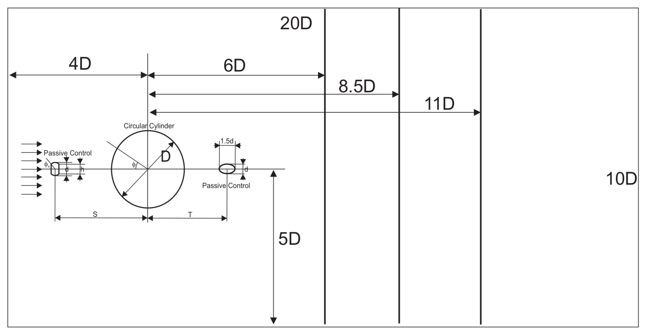
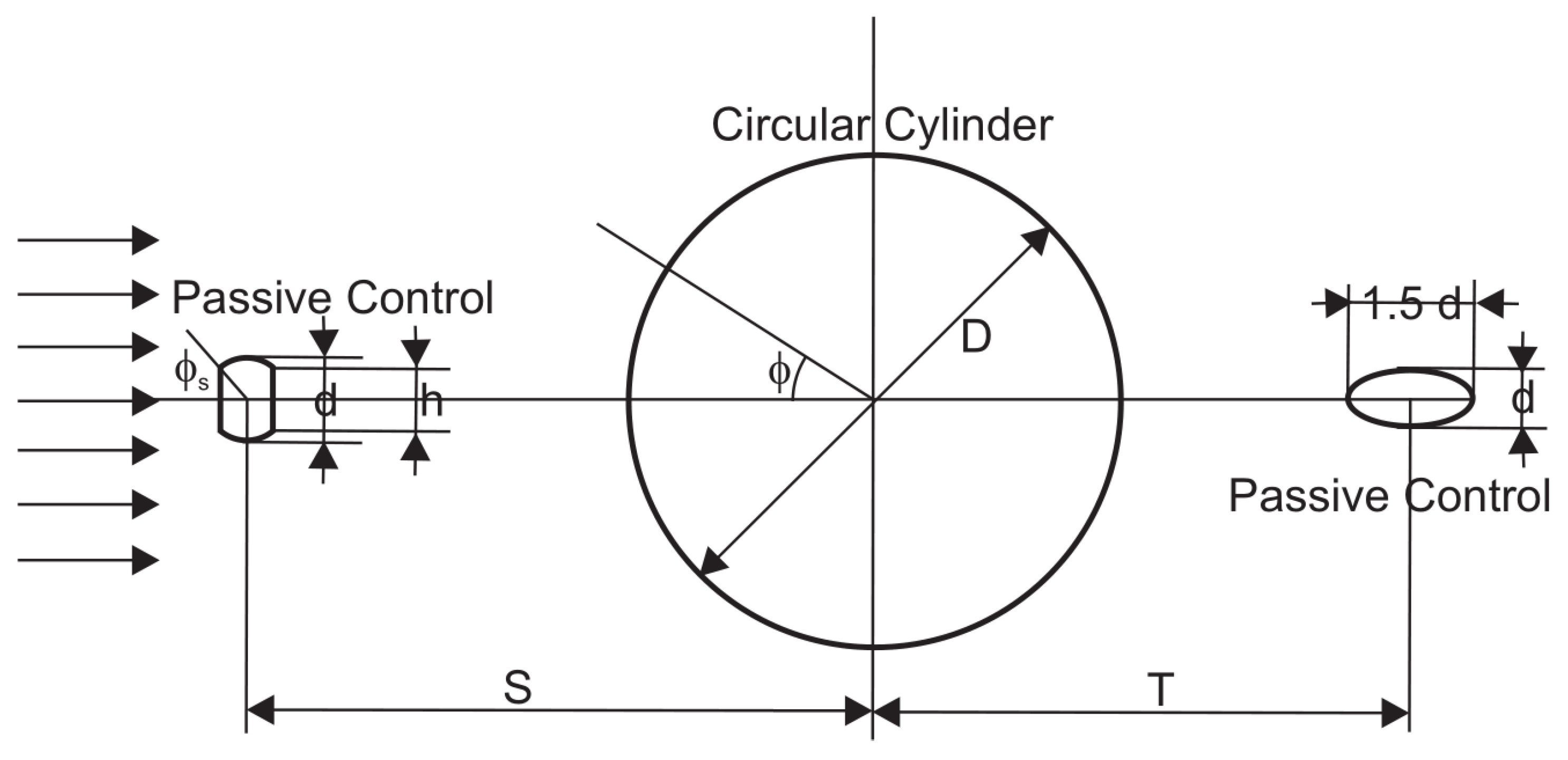
Our research system is 10 D × 20 D . The circular cylinder is placed at a distance 4 D from the front of the system and in the center of the system as in Figure 2. Beside that, we use two passive controls. The first passive control is the Type-I cylinder placed in front of the circular cylinder at various distances, i.e., S / D = 0.6 , 1.2, 1.8, 2.4 and 3.0. The second passive control is an elliptical cylinder placed at the rear of the circular cylinder at various distances, i.e., T / D = 0.6 , 0.9, 1.2, 1.5, 1.8 and 2.1, as in Figure 3. We simulated the experiment by using C++, while plotted the model by using MATLAB R2013a.

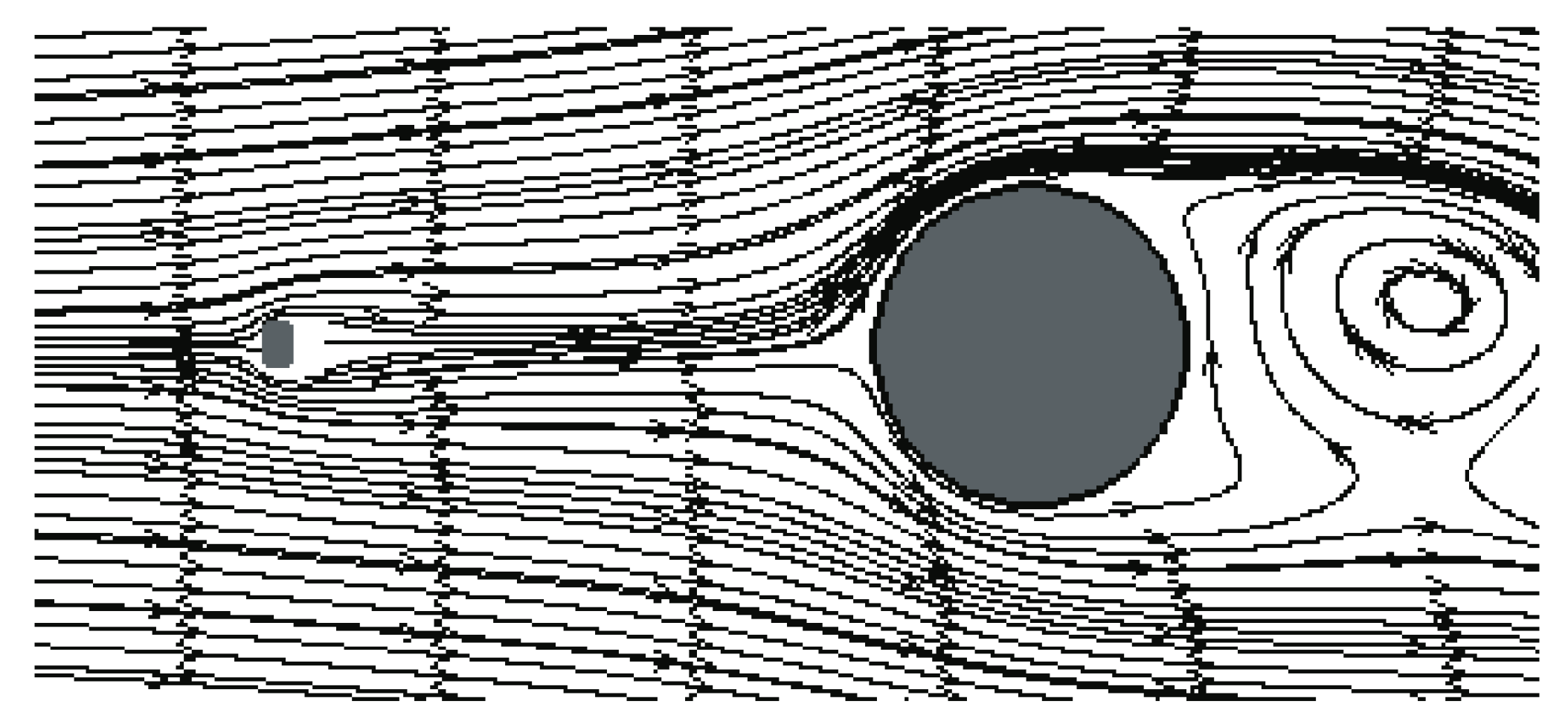
3.1. Single Passive Control

A passive control is a steady device used to reduce drag in the fluid flow. In our research, a passive control placed in front of the main object is a circular cylinder cut on the left and right side with a cutting angle of 53 so that it looks like an I, i.e., the type-I cylinder, as in Figure 4. It is placed perpendicular to the incoming flow at various distances S / D and in a line with a front stagnation point.
When the fluid flows, it will hit the passive control first. The passive control also acts as a turbulence generator. The drag coefficient is high at S / D = 0.6 . This is caused by the turbulence produced by the passive control directly hitting the circular cylinder as the main object. When the distance between the passive control and circular cylinder ( S / D ) is larger, the direct hit turbulence is decreased such that the drag coefficient is reduced and maximum at S / D = 2.4 . When the value of S / D is larger than 2.4, the turbulence disappears and changes to laminar flow with the increasing velocity such that the drag coefficient is increased. Table 1 shows the drag coefficient of a circular cylinder with various distances using a passive control Type-I cylinder placed in front. The best distance obtaining the minimum drag coefficient is S / D = 2.4 with the value of 0.894. The small value of drag coefficient shows that the received drag by the fluid flow is small. By using a passive control in front of the main object, the drag coefficient is reduced from 1.21 down to 0.894 with S / D = 2.4 at R e = 1000 . Hence, adding a passive control in front of circular cylinder is better than without passive control.

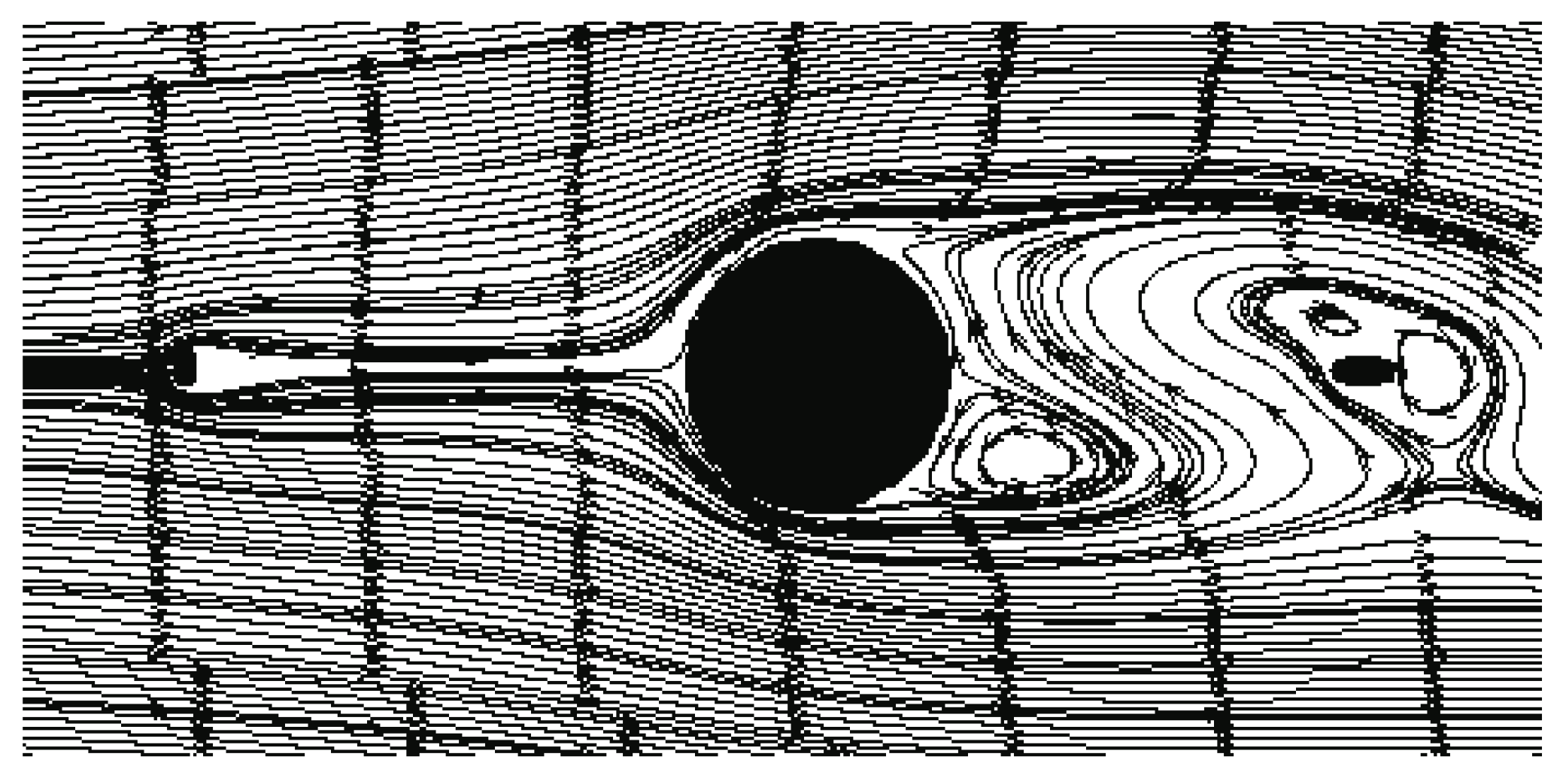
3.2. Two Passive Controls

Besides a passive control placed in front of the main object, we used another passive control placed at the rear of the main object. Another passive control is the elliptical cylinder. It is horizontal and in a line with the rear stagnation point as in Figure 5. The size of the elliptical cylinder can be seen in Figure 3.
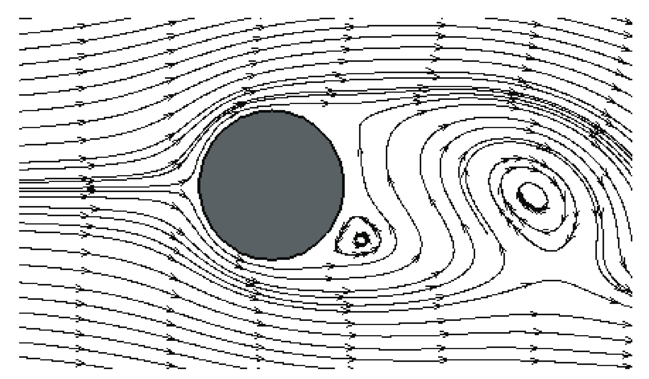
When the fluid flow passes the circular cylinder, it causes downstream disturbance, called wake. The wake is produced at some distance at the rear of the circular cylinder. In order to reduce the drag coefficient, an elliptical cylinder is placed as the passive control at the rear of the circular cylinder. The small T / D makes no significant change to the drag coefficient with various S / D . When the value of T / D is increasing, it has the maximum reducing drag coefficient with configuration S / D = 2.4 and T / D = 2.1 , as shown in Table 2. This means that at T / D = 2.1 , the wake is produced. The position of an elliptical cylinder at T / D = 2.1 breaks the wake forming. Hence, the drag coefficient is reduced from 0.894 down to 0.824. It can be concluded that using two passive controls is better than using one passive control.

3.3. Mathematical Modeling

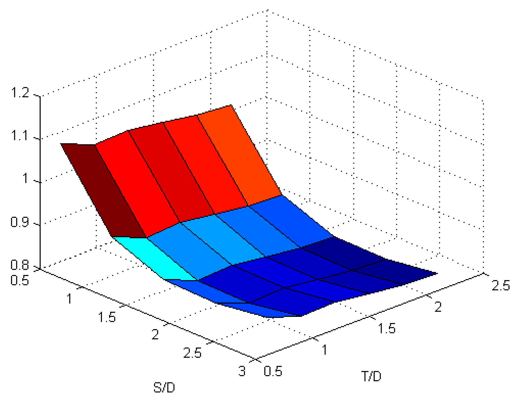
Mathematical modeling is a way to allow a phenomenon to be written in mathematical language, usually called a mathematical model. The obtained model may help to make a prediction about the behavior of a phenomenon. Therefore, the phenomenon of the drag coefficient reduction as shown in Table 2 can be predicted at other points by using its model without creating its program.
Table 2 can be plotted as Figure 6. Let us consider S / D as x, T / D as y and C d as z. Because there are two variables, bilinear interpolation can be used. Assume z i , j = ( x i , y j ) where i = 1 , , 5 and j = 1 , , 6 . First, we do linear interpolation in the x-direction.
f ^ ( x , y 1 ) = l 5 , 1 ( x ) z 1 , 1 + l 5 , 2 ( x ) z 2 , 1 + + l 5 , 5 ( x ) z 5 , 1 = i , k = 1 5 l 5 , k ( x ) z i , 1 f ^ ( x , y 6 ) = l 5 , 1 ( x ) z 1 , 6 + l 5 , 2 ( x ) z 2 , 6 + + l 5 , 5 ( x ) z 5 , 6 = i , k = 1 5 l 5 , k ( x ) z i , 6
or it can be written as:
f ^ ( x , y j ) = i , k = 1 5 L 5 , k z i , j
where for k = 1 , , 5 ,
l 5 , k ( x ) = x x 1 x k x 1 x x k 1 x k x k 1 x x k + 1 x k x k + 1 x x 5 x k x 5
Then, we proceed with the linear interpolation in the y-direction:
f ^ ( x , y ) = h 6 , 1 ( y ) f ( x , y 1 ) + h ( 6 , 2 ) ( y ) f ( x , y 2 ) + + h 6 , 5 ( y ) f ( x , y 6 ) = j , k = 1 5 h 6 , k ( y ) f ( x , y j )
where for k = 1 , , 6 ,
h 6 , k ( y ) = y y 1 y k y 1 y y k 1 y k y k 1 y y k + 1 y k y k + 1 y y 6 y k y 6
Assume Z 6 × 5 = z j , i , H 1 × 6 = h 1 , j and L 5 × 1 = l i , 1 , then Equation (9) can be written as:
f ^ ( x , y ) = H 1 × 6 Z 6 × 5 L 5 × 1
By substituting every point in Table 2 into Equation (10), we obtain:
f ^ ( x , y ) = 12500 729 y 5 10000 81 y 4 + 27875 781 y 3 4150 9 y 2 + 2645 9 y 70 95 7776 x 4 1 8 x 3 + 2159 4320 x 2 359 400 x + 36 25 + 12500 729 y 5 + 250 27 y 4 14375 81 y 3 + 425 3 y 2 350 3 y
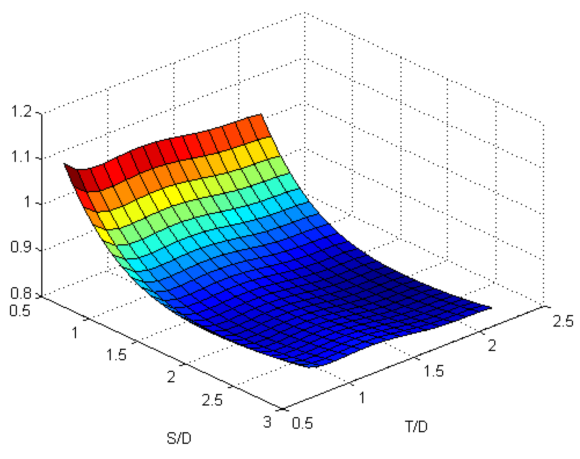
The plot of the equation above can be seen in Figure 7. The range value of S / D is between 0.6 and 3.0, while the range value of T / D is between 0.6 and 2.1. The meshing size used is 25 × 16 . The best drag coefficient reduction by using Equation (11) is 0.822 with the configuration S / D = 2.0 or S / D = 2.2 and T / D = 2.1 . Equation (11) is only used with the configuration S / D between 0.6 and 3.0 and T / D between 0.6 and 2.1. If the value of S / D and T / D is far from the points of those approximated, the value of C d is not true.
Let f ( x , y ) be the function approximated with bilinear interpolation, then:
f ( x , y ) = f ^ ( x , y ) + R ( x , y )
where R ( x , y ) is the remainder, which can be written as:
R ( x , y ) = f ξ ( x , y ) ( m + n ) m ! n ! ( x x 1 ) ( x x 2 ) ( x x m ) ( y y 1 ) ( y y 2 ) ( y y n )
with m the number of points on the x-axes and n the number of points on the y-axes. As a consequence,
R ( x , y ) = 1 5 ! 6 ! f 11 ξ ( x , y ) x 5 y 6 ( x 0.6 ) ( x 1.2 ) ( x 1.8 ) ( x 2.4 ) ( x 3 ) ( y 0.6 ) ( y 0.9 ) ( y 1.2 ) ( y 1.5 ) ( y 1.8 ) ( y 2.1 )
where x [ 0.6 , 3 ] and y [ 0.6 , 2.1 ] .

4. Conclusions

The drag coefficient is significantly decreased when two passive controls are given. This is better for reducing the drag coefficient than one passive control or without passive control. The best reduction of the drag coefficient depends on its position. The best position is at S / D = 2.4 and at T / D = 2.1 with the drag coefficient value of 0.824. By using the mathematical model, the best drag coefficient is 0.822 with the configuration at S / D = 2.0 and T / D = 2.1 or S / D = 2.2 and T / D = 2.1 . If the value of chosen S / D and T / D is far from their range when plotted by using bilinear interpolation, the value of the drag coefficient may not be true.

Acknowledgments

We appreciate the head of the Research and Community Service Institut Teknologi Sepuluh Nopember (LPPM ITS), Surabaya, Indonesia, on behalf of the Ministry of Technology and Higher Education (Kemenristekdikti), who has given us a research grant under Contract No. 010/SP2H/LT/DRPM/IV/2017, 20 April 2017, giving us the opportunity to disseminate our research in this paper.

Author Contributions

Chairul Imron created, designed and performed the simulation of the experiment; Lutfi Mardianto created the mathematical model and wrote the paper; Basuki Widodo and Tri Yogi Yuwono analyzed the data of simulation and mathematical model.

Conflicts of Interest

The authors declare no conflict of interest.

Abbreviations

The following abbreviations are used in this manuscript:
ReReynolds number
vVector velocity
PPressure
SORSuccessive over relaxation
DDiameter of circular cylinder
PCPassive control

References

  1. Ladjedel, A.O.; Yahiaoui, B.T.; Adjlout, C.L.; Imine, D.O. Experimental and numerical studies of drag reduction on circular cylinder. World Acad. Sci. Eng. Technol. 2011, 77, 357–361. [Google Scholar]
  2. Igarashi, T.; Shiba, Y. Drag reduction for D-shape and I-shape cylinder (aerodynamics mechanism of reduction drag). JSME Int. J. Ser. B 2006, 49, 1036–1042. [Google Scholar] [CrossRef]
  3. Yuwono, T.; Widodo, W.A. Flow characteristics around a D-type cylinder near a plane wall. In Proceedings of the Regional Conferences on Mechanical and Aerospace Technology, Bali, Indonesia, 9–10 February 2010. [Google Scholar]
  4. Bouak, F.; Lemnay, J. Passive control of the aerodynamics forces acting on circular cylinder. Exp. Therm. Fluid Sci. 1998, 16, 112–121. [Google Scholar] [CrossRef]
  5. Tsutsui, T.; Igarashi, T. Drag reduction of a circular cylinder in an air stream. J. Wind Eng. Ind. Aerodyn. 2002, 90, 527–541. [Google Scholar] [CrossRef]
  6. Yuwono, T.; Nuh, M. Using of bluff body cut from a circular cylinder as a passive control to reduce aerodynamics forces on a circular cylinder. In Proceedings of the International Conference on Fluid and Thermal Energy Conversion, Bali, Indonesia, 7–11 December 2003. [Google Scholar]
  7. Lee, S.-J.; Lee, S.-I.; Park, C.-W. Reducing the drag on a circular cylinder by upstream installation of small control rod. Fluid Dyn. Res. 2004, 34, 233–250. [Google Scholar] [CrossRef]
  8. Oruc, V. Passive control of flow structures around a circular cylinder by using screen. J. Fluids Struct. 2012, 33, 229–242. [Google Scholar] [CrossRef]
  9. Imron, C.; Yunus, M. Mathematical modelling of pressure on cylindrical ellipse using side-by-side configuration. Int. J. Comput. Sci. Appl. Math. 2015, 1, 10–11. [Google Scholar] [CrossRef]
  10. Widodo, B. The influenced of hydrodynamics on pollutant dispersion in the river. Int. J. Contemp. Math. Sci. 2012, 7, 2229–2234. [Google Scholar]
  11. Imron, C.; Widodo, B.; Yuwono, T. Effectiveness of passive control to reduce the drag coefficient. J. Phys. Conf. Ser. 2017, 890, 012044. [Google Scholar] [CrossRef]
  12. Aiba, S.; Watanabe, H. Flow characteristics of a bluff body cut from a circular cylinder. J. Fluids Eng. 1997, 119, 453–457. [Google Scholar] [CrossRef]
  13. Imron, C.; Widodo, B.; Yuwono, T. Numerical simulation of fluid flow around circular cylinder and I-shape cylinder in a tandem configuration. Appl. Math. Sci. 2013, 7, 5657–5666. [Google Scholar] [CrossRef]
Figure 1. Fluid flow passing a circular cylinder without passive control.
Mca 23 00002 g001
Figure 2. Designed research system.
Mca 23 00002 g002
Figure 3. Schematic of two passive controls and a circular cylinder.
Mca 23 00002 g003
Figure 4. Type-I circular cylinder as a passive control at the front of the main object.
Mca 23 00002 g004
Figure 5. Type-I circular cylinder as a passive control in front, while an elliptical cylinder as a passive control at the rear of the circular cylinder.
Mca 23 00002 g005
Figure 6. Real data plot of the drag coefficient.
Mca 23 00002 g006
Figure 7. Mathematical model plot of the reduction of the drag coefficient.
Mca 23 00002 g007
Table 1. C d of a circular cylinder with a passive control.
S/D0.61.21.82.43.0
C d 1.1140.9460.8960.8940.911
Table 2. C d of the circular cylinder with two passive controls.
C d S/D
T/D0.61.21.82.43.0
0.61.0900.9230.8740.8720.889
0.91.0560.8920.8430.8420.860
1.21.0610.8960.8470.8460.863
1.51.0490.8850.8370.8260.853
1.81.0360.8740.8280.8270.844
2.11.0290.8700.8250.8240.841

