An Algorithmic Comparison of the Hyper-Reduction and the Discrete Empirical Interpolation Method for a Nonlinear Thermal Problem

Abstract

A novel algorithmic discussion of the methodological and numerical differences of competing parametric model reduction techniques for nonlinear problems is presented. First, the Galerkin reduced basis (RB) formulation is presented, which fails at providing significant gains with respect to the computational efficiency for nonlinear problems. Renowned methods for the reduction of the computing time of nonlinear reduced order models are the Hyper-Reduction and the (Discrete) Empirical Interpolation Method (EIM, DEIM). An algorithmic description and a methodological comparison of both methods are provided. The accuracy of the predictions of the hyper-reduced model and the (D)EIM in comparison to the Galerkin RB is investigated. All three approaches are applied to a simple uncertainty quantification of a planar nonlinear thermal conduction problem. The results are compared to computationally intense finite element simulations.

1. Introduction

Numerical models in engineering or natural sciences are getting more and more complex, may be nonlinear and depending on unknown or controllable design-parameters. Simultaneously, simulation settings increasingly move from single-forward simulations to higher-level simulation scenarios. For example, optimization and statistical investigations require multiple solves, interactive applications require real-time simulation response, or slim-computing environments, e.g., simple controllers, require rapid and memory-saving models. For such applications, the field of model reduction has gained increasing attention during the last decade. Their goal is an acceleration of a given numerical model based on the construction of a low-dimensional approximate surrogate model, the so-called reduced order model. Due to the reduced dimension, the computation should ideally be rapid, hence be applicable for the mentioned multi-query, real-time or slim-computing simulation scenarios. Well-known techniques for linear problems comprise Proper Orthogonal Decomposition (POD) [1,2], control-theoretic approaches such as Balanced Truncation, Moment Matching or Hankel-norm approximation [3]. For parametric problems, certified Reduced Basis (RB) methods have been developed [4,5]. Nonlinear problems pose additional challenges. In particular, there exists a well-known drawback with POD, which is that a high-dimensional reconstruction of the reduced solution is required for each evaluation of the nonlinearity. Several approximation techniques exist, which provide a remedy of this problem. Mainly, these approaches are sampling-based techniques such as Empirical Interpolation [6] and discrete variants [7,8,9,10] or Hyper-Reduction [11,12]. Note that also further approaches exist, such as Gappy-POD [13], Missing Point Estimation (MPE) [14] or Gauss–Newton with approximated Tensors (GNAT) [15] and Energy Conserving Mesh Sampling and Weighting (ECSW) [16]. Most of those methods identify a subset of the arguments of the nonlinear function. Then, based solely on an evaluation of these few components, they construct an approximation of the full solution.

Nonlinear problems emerge in many applications. For instance, the effective behavior of dissipative microstructured materials needs to be predicted by nonlinear homogenization techniques. These imply a multi-query context in the sense of different loadings (and load paths) applied to the reference volume element in order to obtain the related effective mechanical response. Reduced basis methods combining the purely algorithmic gains of the reduced basis with a reformulation of the problem incorporating micromechanics have shown to be efficient for the prediction of the effective material response, for multi-level FE simulations and for nonlinear multiscale topology optimization (e.g., [17,18]).

In this paper, we analyze and compare two of those efficient methods, namely Discrete Empirical Interpolation (DEIM) and Hyper-Reduction (HR), for the reduction of a non-trivial nonlinear parametric thermal model. The comparison is carried out on the numerical, algorithmical and mathematical level. A new condition for which DEIM and HR are equivalent is given and numerical examples illustrate the application. Similar studies, often with stronger emphasis on the performance, have also been recently conducted by other authors, e.g., [19].

The paper is structured as follows. We introduce the nonlinear parametrized thermal model problem in Section 2. Subsequently, in Section 3, the methods under investigation are introduced and formally compared: as a benchmark, the POD–Galerkin procedure is formulated, then the DEIM and the hyper-reduction technique. The numerical comparison is provided in Section 4. A classical scenario from uncertainty quantification is demonstrated since model order reduction is particularly interesting for such many-query scenarios. Finally, we conclude in Section 5.

1.1. Nomenclature

In the manuscript, the following notation is used: bold face symbols denote vectors (lowercase letters) or matrices (uppercase letters). The spatial gradient operator is denoted by $\nabla •$ and the divergence is expressed by $\nabla ·•$. The dependence on spatial coordinates is omitted for simplicity of notation.

2. Nonlinear Reference Problem

2.1. Strong Formulation

In the following, we consider a stationary planar nonlinear heat conduction problem on a plate with a hole (see Figure 1). The problem is parametrized by a vector p. The nonlinearity of the problem is introduced by an isotropic Fourier-type heat conductivity $\mu (u;\mathit{p})$ that depends on the current temperature u and the parameter vector. The Dirichlet and Neumann boundary data are denoted by $u_{*}$ and $q_{*}$, respectively. Note that, in the example, $q_{*}=0$ is considered. However, the formulation of the weak form is considered with $q_{*}$ being arbitrary for the sake of generality. The corresponding Dirichlet and Neumann boundaries are denoted by ${\Gamma }_1$ and ${\Gamma }_2$, respectively. The strong formulation of the boundary value problem is

$$\begin{array}{cccccc}\hfill -\nabla ·\left(\mu (u;\mathit{p})\nabla u\right)& =0\mathrm{in}\Omega ,\hfill & \hfill u& =u_{*}\left(\mathit{p}\right)\mathrm{on}{\Gamma }_1,\hfill & \hfill -\mu (u;\mathit{p})\nabla u·\mathit{n}& =q_{*}\mathrm{on}{\Gamma }_2,\hfill \end{array}$$

(1)

where $\mu$ is the temperature dependent conductivity.

2.2. Weak Formulation

The weak form of the heat conduction problem (1) is given by

$$\begin{array}{cc}\hfill a(u,\delta u;\mathit{p})-l(\delta u;\mathit{p})& =0(\forall \delta u\in {\mathcal{V}}_0),\hfill \end{array}$$

(2)

where

$$\begin{array}{c}\hfill a(u,\delta u;\mathit{p})=\underset{\Omega }{\int }\mu (u;\mathit{p})\nabla u·\nabla \delta u\mathrm{d}\Omega ,\mathrm{and}l(\delta u;\mathit{p})=-\underset{{\Gamma }_2}{\int }\delta u{q}_{*}\mathrm{d}\Gamma ,\end{array}$$

(3)

with the unknown temperature field $u\in \mathcal{V}={\mathcal{V}}_0+\left\{{\overline{u}}_{*}\left(\mathit{p}\right)\right\}$ being sought-after. The function space ${\mathcal{V}}_0:=\{u\in {\mathcal{H}}^1\left(\Omega \right):u=0\mathrm{on}{\Gamma }_1\}$ is referred to as space of test functions vanishing on the Dirichlet boundary ${\Gamma }_1$ and ${\overline{u}}_{*}\left(\mathit{p}\right)\in {\mathcal{H}}^1\left(\Omega \right)$ is a field defined on the full domain that satisfies the Dirichlet conditions. The Dirichlet conditions on ${\Gamma }_1$ are assumed to depend on two parameters $g_{\mathrm{x}}$ and $g_{\mathrm{y}}$ via

$$\begin{array}{cc}\hfill u_{*}\left(\mathit{p}\right)& :=g_{\mathrm{x}}x+g_{\mathrm{y}}y,g_{\mathrm{x}},g_{\mathrm{y}}\in [0,1],x,y\in {\Gamma }_1.\hfill \end{array}$$

(4)

A trivial choice is to set ${\overline{u}}_{*}\left(\mathit{p}\right)=g_{\mathrm{x}}x+g_{\mathrm{y}}y$ in the full domain. This particular choice is considered in the remainder of this study. While the solution space $\mathcal{V}$ depends on the parameters p via ${\overline{u}}_{*}$, the space of test functions ${\mathcal{V}}_0$ is independent of the parameters p. For the heat conductivity $\mu$, an explicit dependence on the temperature via the nonlinear constitutive model

$$\begin{array}{cc}\hfill \mu (u;\mathit{p})& :=\max \left\{{\mu }_1,{\mu }_0+cu\right\}\hfill \end{array}$$

(5)

is assumed (see also Figure 1, right). The parameter vector p in the present context is

$$\begin{array}{cc}\hfill \mathit{p}& :=[g_{\mathrm{x}},g_{\mathrm{y}},c,{\mu }_0,{\mu }_1],\hfill \end{array}$$

(6)

and attention will be confined to the compact parameter domain

$$\begin{array}{cc}\hfill \mathit{p}& \in \mathcal{P}:=[0,1]\times [0,1]\times [1,2]\times \left\{1\right\}\times \left\{0.5\right\}\subset {\mathbb{R}}^5.\hfill \end{array}$$

(7)

2.3. Discrete Formulation

In order to solve the nonlinear problem (1), nodal Finite Elements (FE) are used in a classical Galerkin formulation (e.g., [20,21]). The space of finite element test functions ${\mathcal{V}}_0^{\mathrm{h}}\subset {\mathcal{V}}_0$ is assumed to be spanned by n linearly independent and continuous ansatz functions ${\phi }_i$ associated with nodes $(x_i,y_i)$ and ${\phi }_i(x_j,y_j)={\delta }_{ij}$ where $i,j=1,\dots ,n$. We assume a solution expansion into a linear field ${\overline{u}}_{*}$ defined over the full domain $\Omega$ via (4) and comply to the parameterized boundary data and a fluctuation term according to

$$\begin{array}{cccc}\hfill u_h\left(\mathit{p}\right)& :={\overline{u}}_{*}\left(\mathit{p}\right)+\sum _{j=1}^n{w}_{h,j}\left(\mathit{p}\right){\phi }_j,\hfill & \hfill {\overline{u}}_{*}\left(\mathit{p}\right)& :=g_{\mathrm{x}}x+g_{\mathrm{y}}y\forall x,y\in \Omega .\hfill \end{array}$$

(8)

Here, the coefficient vector $\mathit{w}\left(\mathit{p}\right)={\left(w_{h,j}\left(\mathit{p}\right)\right)}_{j=1}^n\in {\mathbb{R}}^n$ contains the nodal temperature fluctuations, which represent the unknowns of the system. They define the coefficient vector containing the nodal temperatures via

$$\begin{array}{cc}\hfill \mathit{u}(\mathit{w};\mathit{p})& =\mathit{w}\left(\mathit{p}\right)+{\overline{\mathit{u}}}_{*}\left(\mathit{p}\right),\hfill \end{array}$$

(9)

where ${\overline{\mathit{u}}}_{*}\left(\mathit{p}\right)$ is the vector composed of the nodal values of the superimposed linear field ${\overline{u}}_{*}\left(\mathit{p}\right)$. The discrete nonlinear equations that have to be solved for any given parameter vector p are given by

$$\begin{array}{cc}\hfill r_i(\mathit{w};\mathit{p})& :=a\left({\overline{u}}_{*}\left(\mathit{p}\right)+\sum _{j=1}^n{w}_{h,j}{\phi }_j,{\phi }_i;\mathit{p}\right)-l({\phi }_i;\mathit{p})=0\left(\forall i\in \{1,\cdots ,n\}\right).\hfill \end{array}$$

(10)

In our specific numerical example, the linear functional $l({\phi }_i;\mathit{p})$ is zero due to the chosen homogeneous Neumann conditions. However, problem (10) still has a nontrivial solution due to the inhomogeneous Dirichlet data provided through ${\overline{u}}_{*}\left(\mathit{p}\right)$. Condition (10) can be expressed in a compact representation using the vector notation

$$\begin{array}{cc}\hfill r(w;\mathit{p})& :={\left(r_i(w;\mathit{p})\right)}_{i=1}^n=0.\hfill \end{array}$$

(11)

In order to solve the nonlinear problem (11), expressed component-wise in (10), the finite element method is used to provide the functions for the expansion (8). In the following, N denotes a row vector of finite element ansatz functions for the temperature, and G and ${\mathit{G}}^T$ are the discrete gradient and divergence matrices, respectively. The FE approximation of the temperature u and its gradient $\nabla u$ are given by

$$\begin{array}{cc}\hfill u_h(\mathit{w};\mathit{p})& =\mathit{N}\mathit{u}(\mathit{w};\mathit{p})=\mathit{N}\mathit{w}\left(\mathit{p}\right)+\mathit{N}{\overline{\mathit{u}}}_{*}\left(\mathit{p}\right),\hfill \end{array}$$

(12)

$$\begin{array}{cccc}\hfill \nabla u_h(\mathit{w};\mathit{p})& =\mathit{G}\mathit{u}(\mathit{w};\mathit{p})=\mathit{G}\mathit{w}\left(\mathit{p}\right)+\overline{\mathit{g}}\left(\mathit{p}\right),\hfill & \hfill \overline{\mathit{g}}\left(\mathit{p}\right)& =\left[\begin{array}{c}{g}_{\mathrm{x}}\\ g_{\mathrm{y}}\end{array}\right].\hfill \end{array}$$

(13)

Then, the exact Jacobian of the finite element system is

$$\begin{array}{cc}\hfill {\mathit{J}}_{*}(\mathit{w};\mathit{p})& {\displaystyle =\underset{\Omega }{\int }\mu (u_h(\mathit{w};\mathit{p});\mathit{p}){\mathit{G}}^T\mathit{G}+\frac{{\displaystyle \partial \mu (u_h(\mathit{w};\mathit{p});\mathit{p})}}{{\displaystyle \partial u_h}}\left({\mathit{G}}^T\mathit{G}\mathit{u}(\mathit{w};\mathit{p})\right)\mathit{N}\mathrm{d}\Omega ,}\hfill \end{array}$$

(14)

where the first part is the classical finite element stiffness matrix and the second part accounts for the thermal sensitivity of the conductivity $\mu$. In the following, a symmetric approximation of ${\mathit{J}}_{*}$ given by

$$\begin{array}{cc}\hfill \mathit{J}(\mathit{w};\mathit{p})& =\underset{\Omega }{\int }\mu (u_h(\mathit{w};\mathit{p});\mathit{p}){\mathit{G}}^T\mathit{G}\mathrm{d}\Omega \hfill \end{array}$$

(15)

is used, i.e., the thermal sensitivity is neglected. The numerical solution of the nonlinear problem (11) is then obtained by a fixed-point scheme using J as an approximation of the differential stiffness matrix ${\mathit{J}}_{*}$. The resulting iteration scheme is commonly referred to as successive substitution (Ref. [22], p. 66). Note also that J is well defined for arbitrary thermal fields, while the exact Jacobian is not defined, or more precisely the Jacobian is semi-smooth, for the critical temperature $u_{\mathrm{c}}=({\mu }_1-{\mu }_0)/c,$ which implies a non-differentiability of the conductivity $\mu$.

Algorithm 1 illustrates the nonlinear finite element solution procedure for the considered problem. The comment lines in the algorithm comprise references to computational costs $c_{\mathrm{reloc}}$ (computation of u and $\nabla u$), $c_{\mathrm{const}}$ (for the constitutive model), $c_{\mathrm{rhs}}$ (linked to the residual computation), $c_{\mathrm{Jac}}$ (related to the Jacobian) and $c_{\mathrm{sol}}$ (for the linear solver). This will become relevant in the comparison section.

Algorithm 1: Finite Element Solution

2.4. Reduced Basis Ansatz

In the following, an m-dimensional basis of global ansatz functions ${\psi }_k$ is considered in the reduced framework, where $m\ll n$ is implicitly asserted in order to obtain an actual model order reduction. The functions ${\psi }_k$ define a linear subspace of ${\mathcal{V}}_0^{\mathrm{h}}$, which can be characterized by a matrix $\mathit{V}=\left(V_{ij}\right)\in {\mathbb{R}}^{n\times m}$ via

$$\begin{array}{ccc}\hfill {\psi }_k& :=\sum _{i=1}^n{V}_{ik}{\phi }_i\hfill & (k=1,\cdots ,m).\hfill \end{array}$$

(16)

The reduced coefficient vector $\mathbf{\gamma }\left(\mathit{p}\right)={\left({\gamma }_k\left(\mathit{p}\right)\right)}_{k=1}^m\in {\mathbb{R}}^m$ defines the temperature fluctations in the reduced setting by the affine relation

$$\begin{array}{cccc}\hfill \tilde{u}\left(\mathit{p}\right)=\tilde{u}(\mathbf{\gamma }\left(\mathit{p}\right);\mathit{p})& :=u_{*}\left(\mathit{p}\right)+\tilde{w}\left(\mathit{p}\right),\hfill & \hfill \tilde{w}\left(\mathit{p}\right)& :=\sum _{k=1}^m{\gamma }_k\left(\mathit{p}\right){\psi }_k.\hfill \end{array}$$

(17)

The corresponding vector of discrete values $\tilde{\mathit{u}}\left(\mathit{p}\right):={\left({\tilde{u}}_j\left(\mathit{p}\right)\right)}_{j=1}^n\in {\mathbb{R}}^n$ of the temperature with respect to the basis of ${\mathcal{V}}_0^{\mathrm{h}}$ is given by the linear relation $\tilde{\mathit{u}}={\overline{u}}_{*}\left(\mathit{p}\right)+\tilde{\mathit{w}}\left(\mathit{p}\right)$ with the coefficient vector $\tilde{w}\left(\mathit{p}\right)=V\mathbf{\gamma }\left(\mathit{p}\right)={\left(\tilde{w}\left(\mathit{p}\right)\right)}_{j=1}^n$ of the reduced fluctuation field. Hence, the reduced fluctuation $\tilde{w}$ can equivalently be expressed as

$$\begin{array}{c}\hfill \tilde{w}\left(\mathit{p}\right)=\sum _{j=1}^n{\tilde{w}}_j\left(\mathit{p}\right){\phi }_j=\sum _{j=1}^n{\phi }_j\sum _{k=1}^m{V}_{jk}{\gamma }_k\left(\mathit{p}\right).\end{array}$$

(18)

In the following, the matrix V defining the space of the reduced ansatz functions is assumed to be given by a snapshot POD [23] obtained from full resolution finite element simulations evaluated at s different parameter vectors ${\mathit{p}}^{\left(i\right)}$ ($i=1,\cdots ,s$). The POD subspace ${\tilde{\mathcal{V}}}_0^{\mathrm{h}}\subset {\mathcal{V}}_0^{\mathrm{h}}$ is then obtained as best-approximating m-dimensional subspace with respect to the $L^2\left(\Omega \right)$-error, i.e.,

$$\begin{array}{cc}\hfill {\tilde{\mathcal{V}}}_0^{\mathrm{h}}& =\underset{\stackrel{\tilde{\mathcal{V}}\subset {\mathcal{V}}_0^{\mathrm{h}}}{\dim (\tilde{\mathcal{V}})=m}}{\arg \min }\sum _{i=1}^s{∥w_h({\mathit{p}}^{\left(i\right)})-P_{\tilde{\mathcal{V}}}(w_h({\mathit{p}}^{\left(i\right)})∥}_{L^2\left(\Omega \right)}^2,\hfill \end{array}$$

(19)

where $P_{\tilde{\mathcal{V}}}$ is the orthogonal projection of the thermal fluctuations onto the subspace $\tilde{\mathcal{V}}$. Numerically, a POD-basis of this space can be obtained by a corresponding matrix eigenvalue problem, e.g., cf. [1,5,24]. Here, we use the $L^2\left(\Omega \right)$ inner product for the computation of the symmetric snapshot inner product matrix

$$\begin{array}{cccc}\hfill \mathit{C}& ={\left(C_{ij}\right)}_{i,j=1}^s\in {\mathbb{R}}^{s\times s},\hfill & \hfill C_{ij}& :=\underset{\Omega }{\int }{w}_h({\mathit{p}}^{\left(i\right)})w_h({\mathit{p}}^{\left(j\right)})\mathrm{d}\Omega .\hfill \end{array}$$

(20)

Note that the correlation matrix is computed from the temperature fluctuations $w_h$ only in order to obtain a reduced basis that will comply with the prescribed Dirichlet conditions that are accounted for in ${\overline{u}}_{*}\left(\mathit{p}\right)$. The entries of C are defined by the discrete snapshot solutions $w^{\left(i\right)}$ via the unit mass matrix M as follows:

$$\begin{array}{cccc}\hfill \mathit{M}& :=\underset{\Omega }{\int }{\mathit{N}}^T\mathit{N}\mathrm{d}\Omega ,\hfill & \hfill C_{ij}& ={\left({\mathit{w}}^{\left(i\right)}\right)}^T\mathit{M}\left({\mathit{w}}^{\left(j\right)}\right).\hfill \end{array}$$

(21)

A pseudo-code implementation of the snapshot POD is given by Algorithm 2. Alternatively, a weighted SVD of the snapshot matrix can be used to obtain the same basis. The classical SVD w.r.t. the $l^2$-norm may be less prone to truncation errors [25], but it will yield a result differing from the optimum in (19), which is based on optimality with respect to ${\parallel ·\parallel }_{L^2\left(\Omega \right)}$. This is due to the missing consideration of the inner product matrix M.

Algorithm 2: Snapshot Proper Orthogonal Decomposition (Snapshot POD)

There are many other techniques to determine reduced projection spaces, e.g., greedy techniques, balanced truncation, Hankel-norm approximation, moment matching and others (e.g., [3]). However, we do not aim at a comparison of projection space techniques, but rather focus on the treatment of the nonlinearities. Therefore, we decide for the POD space as common reduced projection space for all subsequent methods.

Note that, for the given problem, the Dirichlet data can be considered via the linear field ${\overline{u}}_{*}\left(\mathit{p}\right)$ defined in (4). More precisely, ${\overline{u}}_{*}$ is parametrized by two independent parameters $g_{\mathrm{x}}$, $g_{\mathrm{y}}$. Its discrete representation is

$$\begin{array}{c}\hfill {\overline{\mathit{u}}}_{*}\left(\mathit{p}\right)=g_{\mathrm{x}}{\overline{\mathit{u}}}_{*,1}+g_{\mathrm{y}}{\overline{\mathit{u}}}_{*,2},\end{array}$$

(22)

with the components of the vectors ${\mathit{u}}_{*,1}$, ${\mathit{u}}_{*,2}$ defined as

$$\begin{array}{cccc}\hfill {\left(u_{*,1}\right)}_{i=1}^n& :=x_i,\hfill & \hfill {\left(u_{*,2}\right)}_{i=1}^n& :=y_i,\hfill \end{array}$$

(23)

where $x_i$ and $y_i$ denote the coordinates of node number i. By accounting for ${\overline{\mathit{u}}}_{*}\left(\mathit{p}\right)$ via (22), the Dirichlet data is exactly represented without further algebraic constraints. Additionally, this approach captures exactly constant temperature gradients.

3. Sampling-Based Reductions

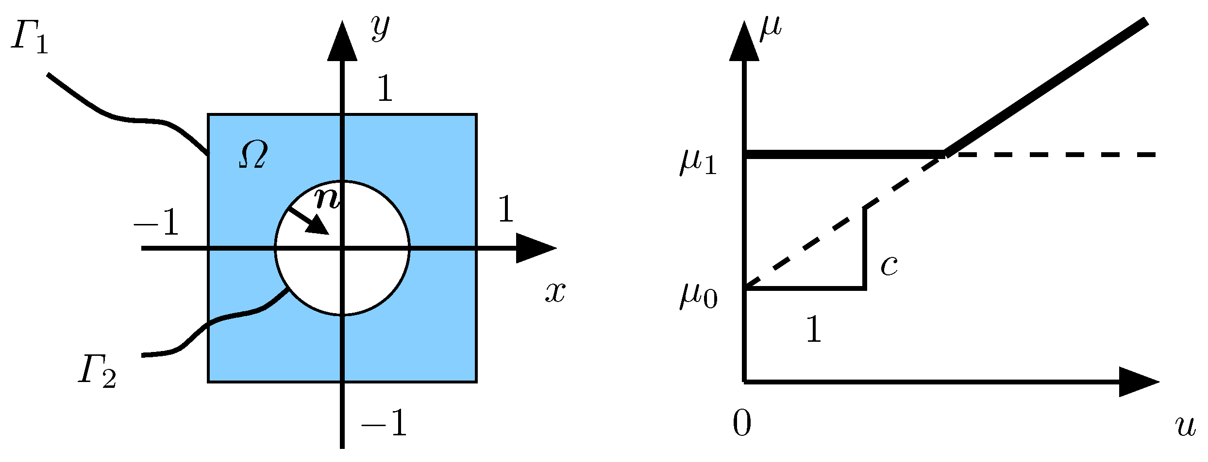
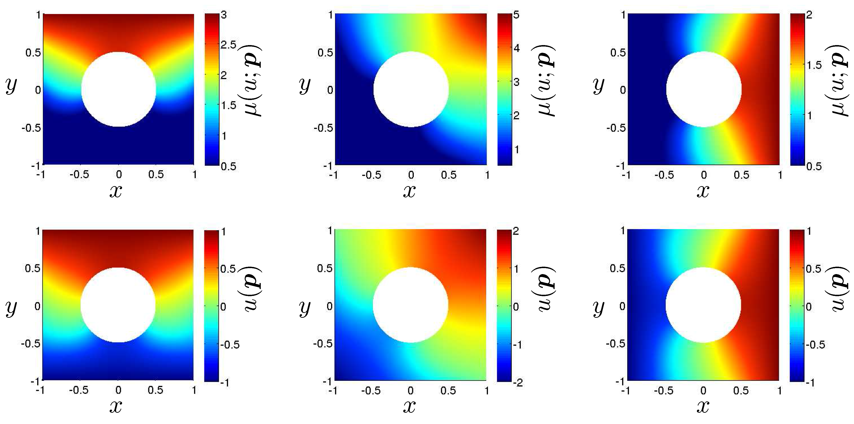
3.1. Galerkin Reduced Basis Approximation

A classical Galerkin projection on a POD space is used to provide reference solutions for the HR and the DEIM. In order to solve the weak form of the nonlinear problem for given parameters $g_{\mathrm{x}}$, $g_{\mathrm{y}}$, a successive substitution is performed in which the local conductivity $\mu$ is computed using the previous iteration of the temperature ${\tilde{u}}^{\left(\alpha \right)}:=u_{*}\left(\mathit{p}\right)+{\tilde{w}}^{\left(\alpha \right)}$ with ${\tilde{w}}^{\left(\alpha \right)}=\mathit{N}\mathit{V}{\mathbf{\gamma }}^{\left(\alpha \right)}$ in the reduced setting, where $\alpha \in \mathbb{N}$ is the iteration number and ${\mathbf{\gamma }}^{\left(\alpha \right)}$ is the iterate of the reduced degrees of freedom in iteration $\alpha$. As in a classical Galerkin approach, we assume the (reduced) test function

$$\begin{array}{cc}\hfill \tilde{v}& :=\sum _{i=1}^n\sum _{j=1}^m{\phi }_i{V}_{ij}{\lambda }_j\hfill \end{array}$$

(24)

with arbitrary coefficients ${\lambda }_j$ ($j=1,\cdots ,m$) represented by the vector $\mathbf{\lambda }$. For convenience, we define the conductivity corresponding to the $\alpha$-th iterate ${\mathbf{\gamma }}^{\left(\alpha \right)}$ of the reduced coefficient vector $\mathbf{\gamma }\left(\mathit{p}\right)$

$$\begin{array}{cc}\hfill {\mu }^{\left(\alpha \right)}& :=\mu \left(\tilde{u}({\mathbf{\gamma }}^{\left(\alpha \right)};\mathit{p});\mathit{p}\right).\hfill \end{array}$$

(25)

Here, ${\mathbf{\gamma }}^{\left(\alpha \right)}$ can be interpreted as a constant parameter similar to p during the subsequent iteration, which provides the new iterate ${\mathbf{\gamma }}^{(\alpha +1)}$ as the solution of

$$\begin{array}{cc}\hfill a(\tilde{u},\tilde{v};\mathit{p})& =\sum _{j=1}^m{\lambda }_j\underset{\Omega }{\int }{\mu }^{\left(\alpha \right)}\nabla \tilde{u}({\mathbf{\gamma }}^{(\alpha +1)};\mathit{p})·\nabla {\psi }_j\mathrm{d}\Omega =0\forall \mathbf{\lambda }\in {\mathbb{R}}^m.\hfill \end{array}$$

(26)

Rewriting (26) using the approximated Jacobian J and the residual r leads to the linear system

$$\begin{array}{cc}\hfill {\mathit{V}}^T\mathit{J}(\mathit{V}{\mathbf{\gamma }}^{\left(\alpha \right)};\mathit{p})\mathit{V}({\mathbf{\gamma }}^{(\alpha +1)}-{\mathbf{\gamma }}^{\left(\alpha \right)})+{\mathit{V}}^T\mathit{r}(\mathit{V}{\mathbf{\gamma }}^{\left(\alpha \right)};\mathit{p})& =0.\hfill \end{array}$$

(27)

The projection of the residual onto the reduced basis defines the reduced residual

$$\begin{array}{cc}\hfill {\tilde{\mathit{r}}}^{\left(\alpha \right)}& :={\mathit{V}}^T\mathit{r}(\mathit{V}{\mathbf{\gamma }}^{\left(\alpha \right)};\mathit{p}).\hfill \end{array}$$

(28)

In view of the definition of the reduced basis by $L^2\left(\Omega \right)$-orthogonal POD modes and with $\delta {\mathbf{\gamma }}^{\left(\alpha \right)}:={\mathbf{\gamma }}^{(\alpha +1)}-{\mathbf{\gamma }}^{\left(\alpha \right)},$ one obtains

$$\begin{array}{cc}\hfill \parallel \delta {\mathbf{\gamma }}^{\left(\alpha \right)}{\parallel }_{l^2}& =\parallel {\tilde{u}}^{(\alpha +1)}-{\tilde{u}}^{\left(\alpha \right)}{\parallel }_{L^2\left(\Omega \right)}=\parallel {\tilde{w}}^{(\alpha +1)}-{\tilde{w}}^{\left(\alpha \right)}{\parallel }_{L^2\left(\Omega \right)}.\hfill \end{array}$$

(29)

This gives rise to the simple convergence criterion $\parallel \delta {\mathbf{\gamma }}^{\left(\alpha \right)}{\parallel }_{l^2}<{ϵ}_{\max }$, i.e., the iteration should stop upon sufficiently small changes of the temperature field. Algorithm 3 summarizes the online phase of the Galerkin RB method.

Algorithm 3: Galerkin Reduced Basis Solution (Online Phase)

The projected system can be interpreted as a finite element method with global, problem specific ansatz functions ${\psi }_k$, whereas the classical finite element method uses local and rather general ansatz functions ${\phi }_j$ (e.g., piecewise defined polynomials).

Note that, the solution of (26), (27) is also a minimizer of the potential

$$\begin{array}{cc}\hfill \mathsf{\Pi }(\mathbf{\gamma };{\mathbf{\gamma }}^{\left(\alpha \right)},\mathit{p})& :={\frac{1}{2}}_{\Omega }{\mu }^{\left(\alpha \right)}\nabla \tilde{u}(\mathbf{\gamma };\mathit{p})·\nabla \tilde{u}(\mathbf{\gamma };\mathit{p})\mathrm{d}\Omega .\hfill \end{array}$$

(30)

Therefore, variational methods can directly be applied to solve the minimization problem and alternative numerical strategies are available. Such variational schemes are also used, e.g., in the context of solid mechanical problems involving internal variables (e.g., [26]).

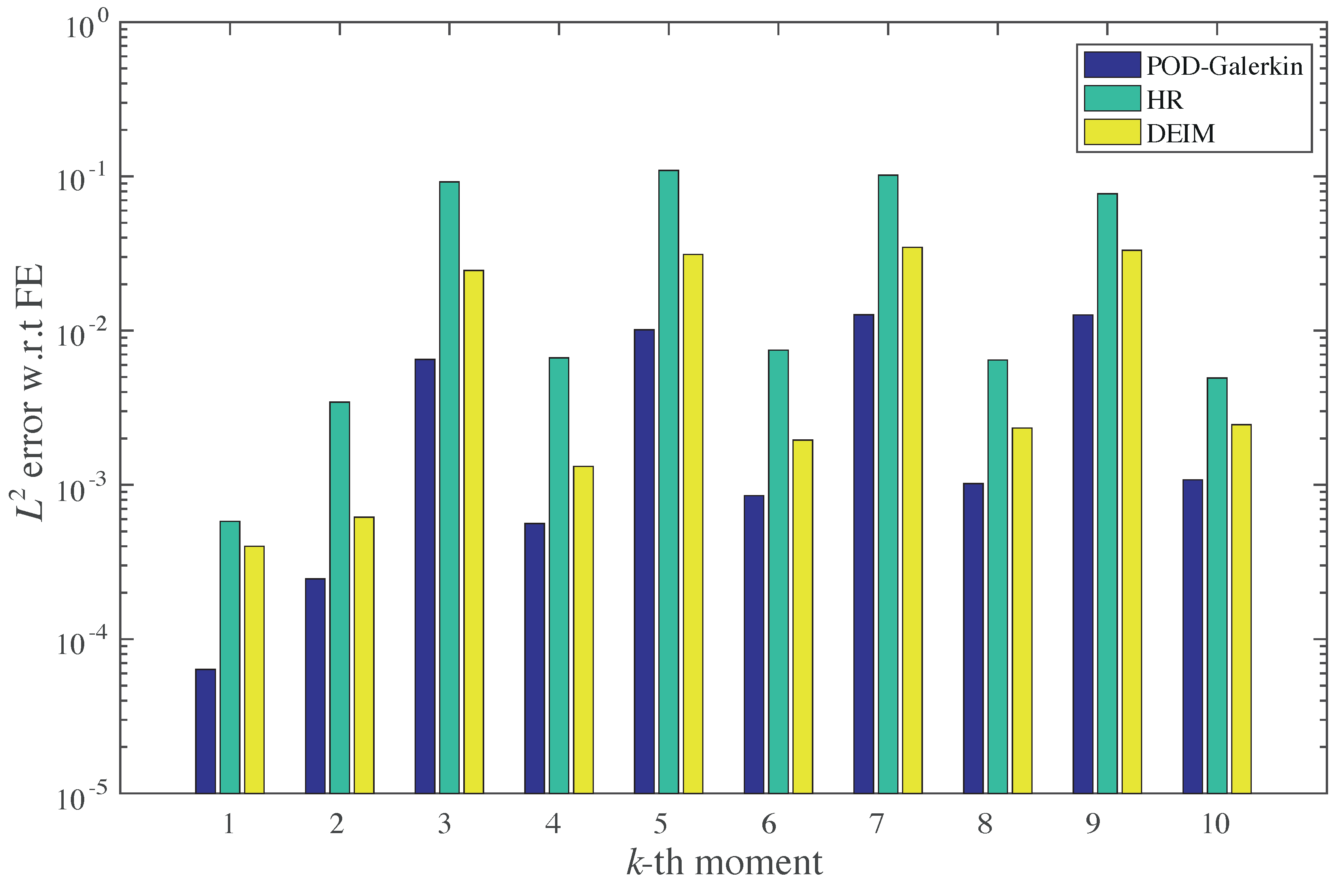
The Galerkin RB method with a well-chosen reduced basis functions ${\psi }_k$ (represented via the matrix V) can replicate the FEM solution to a high accuracy (see Section 4). It also provides a significant reduction of the memory requirements: instead of $\mathit{u}\in {\mathbb{R}}^n$, only $\mathbf{\gamma }\in {\mathbb{R}}^m$ needs to be stored. Despite the significant reduction of the number of unknowns from n to m, the Galerkin RB cannot attain substantial accelerations of the nonlinear simulation due to a computationally expensive assembly procedure with complexity $\mathcal{O}\left(n_{\mathrm{gp}}\right)$ for the residual vector r and for the fixed point operator J (compare $c_{\mathrm{rhs}}$ and $c_{\mathrm{Jac}}$ in Algorithm 1 and Algorithm 3). Here, $n_{\mathrm{gp}}$ is the number of quadrature points in the mesh. However, if the linear systems are not solved with optimal complexity, e.g., using sparse $LU$ or Cholesky decompositions with at least $\mathcal{O}\left(n^2\right)$, then a reduction of complexity can still be achieved. It shall be pointed out that, for very large n (i.e., for millions of unknowns), the linear solver usually dominates the overall computational expense. Then, the Galerkin RB may provide good accelerations without further modifications.

In order to significantly improve on the computational efficiency while maintaining the reduced number of degrees of freedom (and thus the reduced storage requirements), the Hyper-Reduction [11,12] and the Discrete Empricial Interpolation Method (DEIM, [7,8,9]) are used. Both methods are specifically designed for the computationally efficient approximation of the nonlinearity of PDEs.

3.2. Discrete Empirical Interpolation Method (DEIM)

The empirical interpolation method (EIM) was introduced by [6] to approximate parametric or nonlinear functions by separable interpolants. This technique is meanwhile standard in the reduced basis methodology for parametric PDEs. Discrete versions of the EIM for instationary problems have been introduced as empirical operator interpolation [7,8,27] or alternatively (and in some cases equivalently) as discrete empirical interpolation (DEIM) [9,10]. In particular, a posteriori [8,27,28] and a priori [10] error control is possible under certain assumptions (see also [5]).

We present a formulation for the present stationary problem. Instead of approximating a continuous field variable, the goal of the discrete versions is to provide an approximation $\tilde{r}$ for the vectorial nonlinearity of the nodal residual vector r of the form

$$\begin{array}{c}\hfill \tilde{\mathit{r}}(\mathit{u};\mathit{p}):=\mathit{U}{\left({\mathit{P}}^T\mathit{U}\right)}^{-1}{\mathit{P}}^T\mathit{r}(\mathit{u};\mathit{p}),\end{array}$$

(31)

where the columns of $\mathit{U}\in {\mathbb{R}}^{n\times M}$ are called collateral reduced basis and $\mathit{P}=[{\mathit{e}}_{i_1},\dots ,{\mathit{e}}_{i_M}]\in {\mathbb{R}}^{n\times M}$ is a sampling matrix with interpolation indices (also known as magic points) $i_1,\dots ,i_M\in \{1,\dots ,n\}$, with $e_i$ being the i-th unit vector. By multiplication of (31) with $P^T$, we verify that

$$\begin{array}{c}\hfill {\left(\tilde{\mathit{r}}(\mathit{u};\mathit{p})\right)}_{i_j}{=\mathit{r}(\mathit{u};\mathit{p}))}_{i_j},j=1,\dots ,M.\end{array}$$

(32)

In this sense, the approximation acts as an interpolation within the set of magic points.

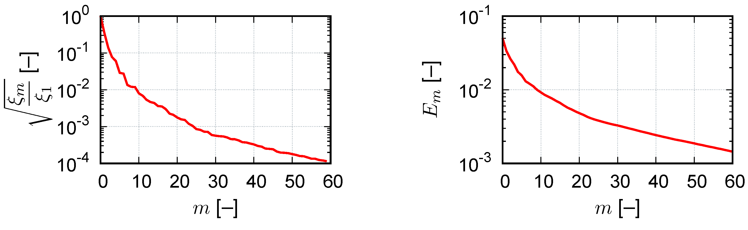
The identification of the interpolation points is an incremental procedure, which is performed during the offline phase. We assume the existence of a set of training snapshots $\mathcal{Y}:=\{y_1,\dots ,y_{n_{\mathrm{train}}}\}\subset {\mathbb{R}}^n$ with $\dim \left(\mathrm{span}\right(\mathcal{Y}\left)\right)\ge M$.

Then, a POD of these snapshots results, see e.g., [10], in the collateral basis vectors ${\mathit{u}}_1,\dots ,{\mathit{u}}_M$ and we define ${\mathit{U}}_l:=[{\mathit{u}}_1,\dots ,{\mathit{u}}_l]$ for $l=1,\dots ,M$. The algorithm for the point selection is initialized with ${\mathit{P}}_0=\left[\right]$, $I_0:=\varnothing$, ${\mathit{U}}_0=\left[\right]$ and then computes for $l=1\dots ,M$

$$\begin{array}{cc}\hfill {\mathit{q}}_l& :={\mathit{u}}_l-{\mathit{U}}_{l-1}{\left({\mathit{P}}_{l-1}^T{\mathit{U}}_{l-1}\right)}^{-1}{\mathit{P}}_{l-1}^T{\mathit{u}}_l,\hfill \end{array}$$

(33)

$$\begin{array}{cc}\hfill i_l& :=\arg \underset{i\in \{1,\dots ,n\}}{max}\left|{\left({\mathit{q}}_l\right)}_i\right|,\hfill \end{array}$$

(34)

$$\begin{array}{cc}\hfill {\mathit{P}}_l& :=[{\mathit{P}}_{l-1},{\mathit{e}}_{i_l}],I_l:=I_{l-1}\cup \left\{i_l\right\}.\hfill \end{array}$$

(35)

Finally, we set $\mathit{P}:={\mathit{P}}_M$, $\mathit{U}:={\mathit{U}}_M$ and $I:=I_M$, which concludes the construction of $\tilde{\mathit{r}}$. Intuitively, in each iteration, the interpolation error ${\mathit{q}}_l$ for the current POD basis vector ${\mathit{u}}_l$ is determined and the vector entry $i_l$ with maximum absolute value is identified, which gives the next index. Regularity of the matrix ${\mathit{P}}^T\mathit{U}$ is required for a well-defined interpolation. This condition is automatically satisfied under the aforementioned assumption of a sufficiently rich set of snapshots $\mathcal{Y}$. As training set $\mathcal{Y}$, one can either use samples of the nonlinearity [8], or use snapshots of the state vector or combinations thereof. In contrast to the instationary case, we may not use only training snapshots of r: As the residual r is zero for all snapshots, we would try to find a basis for a zero-dimensional space $\mathrm{span}\left(\mathcal{Y}\right)=0$, which is not possible for $M>0$. However, the residual at the intermediate (non-equilibrium) iterates is non-zero and this is also a good target quantity for the (D)EIM, as these terms appear on the right-hand side of the linear system during the fixed point iteration. Hence, a reasonable set $\mathcal{Y}$ is obtained via

$$\begin{array}{cc}\mathcal{Y}=[{\mathit{y}}_1,\cdots ,{\mathit{y}}_{n_{\mathrm{train}}}]\hfill & =[\mathit{r}({\mathit{u}}^{\left(0\right)}\left({\mathit{p}}^{\left(1\right)}\right);{\mathit{p}}^{\left(1\right)}),\cdots ,\mathit{r}({\mathit{u}}^{\left({\alpha }_1\right)}\left({\mathit{p}}^{\left(1\right)}\right);{\mathit{p}}^{\left(1\right)}),\hfill \\ & \cdots ,\mathit{r}({\mathit{u}}^{\left({\alpha }_s\right)}\left({\mathit{p}}^{\left(s\right)}\right);{\mathit{p}}^{\left(s\right)})],\hfill \end{array}$$

(36)

where ${\alpha }_1$, ..., ${\alpha }_s$ are the number of fixed point iterations of the full simulation scheme for parameters ${\mathit{p}}^{\left(1\right)},\dots ,{\mathit{p}}^{\left(s\right)}$.

Inserting $\tilde{\mathit{r}}$ from (31) for the nonlinearity into the full problem and projection by left-multiplication with a weight matrix $\mathit{W}\in {\mathbb{R}}^{n\times m}$ yields the POD-DEIM reduced m-dimensional nonlinear system for the unknown $\mathbf{\gamma }$

$$\begin{array}{c}\hfill {\mathit{W}}^T\mathit{U}{\left({\mathit{P}}^T\mathit{U}\right)}^{-1}{\mathit{P}}^T\mathit{r}({\overline{\mathit{u}}}_{*}\left(\mathit{p}\right)+\mathit{V}\mathbf{\gamma };\mathit{p})=0.\end{array}$$

(37)

This low-dimensional nonlinear problem is iteratively solved by a fixed point procedure, i.e., at the current approximation ${\mathbf{\gamma }}^{\left(\alpha \right),}$ we solve the linearized problem for $\delta {\mathbf{\gamma }}^{\left(\alpha \right)}$

$$\begin{array}{c}\hfill {\mathit{W}}^T\mathit{U}{\left({\mathit{P}}^T\mathit{U}\right)}^{-1}{\mathit{P}}^T\mathit{J}({\overline{\mathit{u}}}_{*}\left(\mathit{p}\right)+\mathit{V}{\mathbf{\gamma }}^{\left(\alpha \right)};\mathit{p})\mathit{V}\delta {\mathbf{\gamma }}^{\left(\alpha \right)}=-{\mathit{W}}^T\mathit{U}{\left({\mathit{P}}^T\mathit{U}\right)}^{-1}{\mathit{P}}^T\mathit{r}({\overline{\mathit{u}}}_{*}\left(\mathit{p}\right)+\mathit{V}{\mathbf{\gamma }}^{\left(\alpha \right)};\mathit{p})\end{array}$$

(38)

and set ${\mathbf{\gamma }}^{(\alpha +1)}:={\mathbf{\gamma }}^{\left(\alpha \right)}+\delta {\mathbf{\gamma }}^{\left(\alpha \right)}$. As in the previous sections, if $M<m$, this linear system cannot be solved uniquely. In that case, an alternative would be to solve a residual least-squares problem, similar to the GNAT-procedure, cf. [15]. Note that the assembly of this system does not involve any high-dimensional operations, as the product of the first four matrices on the left- and right-hand side can be precomputed as a small matrix $\mathit{X}:={\mathit{W}}^T\mathit{U}{\left({\mathit{P}}^T\mathit{U}\right)}^{-1}$. Then, the terms ${\mathit{P}}^T\mathit{J},{\mathit{P}}^T\mathit{r}$ also do not require any high-dimensional operations, as the multiplication with ${\mathit{P}}^T(·)={(·)}_I$ corresponds to evaluation of the “magic” rows of the Jacobian and right-hand side, respectively. Typically, in discretized PDEs, these M rows only depend on few $\overline{M}$ entries of the unknown variable (e.g., the DOFs related to neighboring elements). This number $\overline{M}$ is typically bounded by a certain multiple of M due to regularity constraints on the mesh [8].

In (38), what is required for the collateral basis U can be recognized: If $\mathit{J}(\mathit{V}\mathbf{\gamma };\mathit{p})\mathit{V}\delta \mathbf{\gamma }\in \mathrm{colspan}\left(\mathit{U}\right)$ and $\mathit{r}(\mathit{V}\mathbf{\gamma };\mathit{p})\in \mathrm{colspan}\left(\mathit{U}\right),$ then we are exactly solving the Galerkin–POD reduced linearized system

$$\begin{array}{c}\hfill {\mathit{W}}^T\mathit{J}(\mathit{V}\mathbf{\gamma };\mathit{p})\mathit{V}\delta \mathbf{\gamma }=-{\mathit{W}}^T\mathit{r}(\mathit{V}\mathbf{\gamma };\mathit{p}).\end{array}$$

(39)

Hence, this gives a guideline for an alternative reasonable choice of the training set $\mathcal{Y}$, namely consisting of snapshots of both (columns of) J or $\mathit{J}\mathit{V}$ and r.

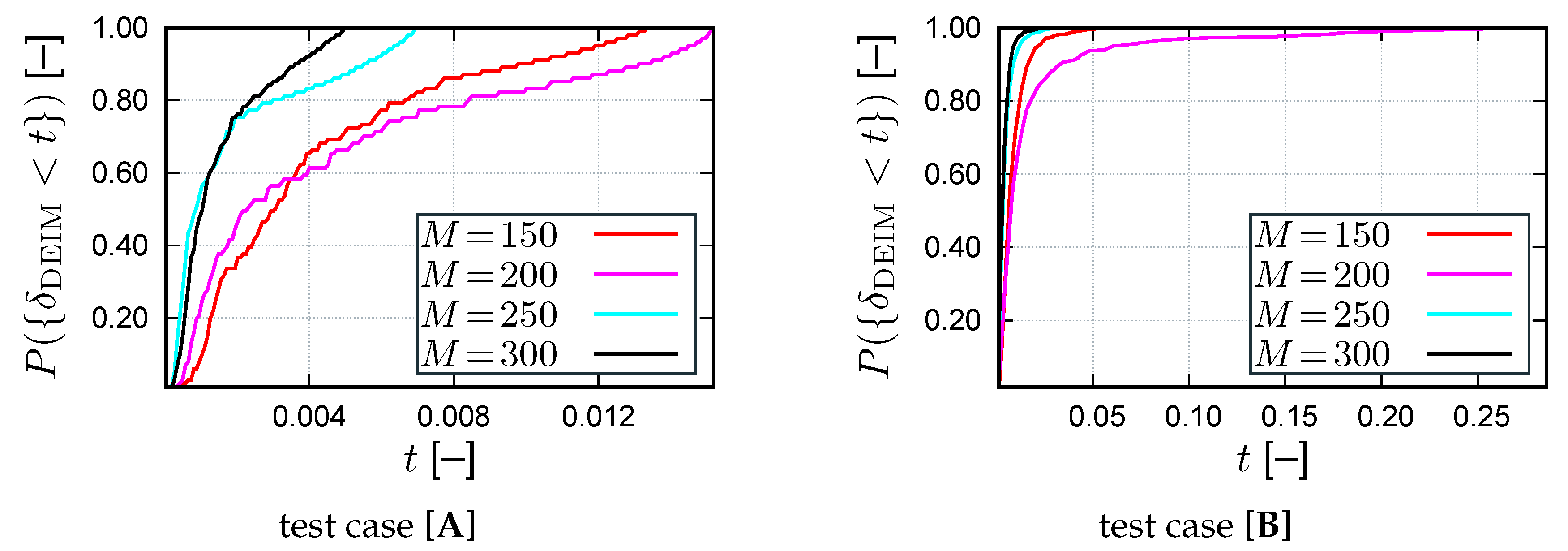
In the Galerkin projection case, one can choose $\mathit{W}=\mathit{V}$. This is the choice that we pursue in the experiments to make the procedure more similar to the other reduction approaches. The offline phase of the DEIM is summarized in Algorithm 4 and an algorithm of the online phase is provided in Algorithm 5.

Algorithm 4: Offline Phase of the Discrete Empirical Interpolation Method (DEIM)

Algorithm 5: Online Phase of the Discrete Empirical Interpolation Method (DEIM)
Input :  parameters $\mathit{p}\in \mathcal{P}$ reduced basis V, POD-DEIM sampling matrix $\mathit{X}:={\mathit{W}}^T\mathit{U}{\left({\mathit{P}}^T\mathit{U}\right)}^{-1}$ and magic point index set I Output:  reduced vector $\mathbf{\gamma }$ and nodal temperatures $\tilde{\mathit{u}}$ (optional)
1 set ${\mathbf{\gamma }}^{\left(0\right)}=0$; ${\tilde{\mathit{u}}}^{\left(0\right)}={\overline{\mathit{u}}}_{*}\left(\mathit{p}\right)$; $\alpha =0$ ;	// initialize
2 $\overline{\mathit{J}}\leftarrow {(\mathit{J}({\tilde{\mathit{u}}}^{\left(\alpha \right)};\mathit{p})\mathit{V})}_I$ ;	// $c_{\mathrm{Jac}}$; evaluate M rows of right-projected Jacobian
3 $\overline{\mathit{r}}\leftarrow {(\mathit{r}({\tilde{\mathit{u}}}^{\left(\alpha \right)};\mathit{p}))}_I$ ;	// $c_{\mathrm{rhs}}$; evaluate M rows of right hand side
4 solve $\mathit{X}\overline{\mathit{J}}\delta {\mathbf{\gamma }}^{\left(\alpha \right)}=-\mathit{X}\overline{\mathit{r}}$ ;	// $c_{\mathrm{sol}}$; fixpoint iter. for $\delta {\mathbf{\gamma }}^{\left(\alpha \right)}$
5 update ${\mathbf{\gamma }}^{(\alpha +1)}\leftarrow {\mathbf{\gamma }}^{\left(\alpha \right)}+\delta {\mathbf{\gamma }}^{\left(\alpha \right)}$;	// update
6 compute ${\mathit{P}}_{\overline{M}}{\tilde{\mathit{u}}}^{(\alpha +1)}\leftarrow {\mathit{P}}_{\overline{M}}{\tilde{\mathit{u}}}^{\left(\alpha \right)}+{\mathit{P}}_{\overline{M}}\mathit{V}\delta {\mathbf{\gamma }}^{\left(\alpha \right)}$ and set $\alpha \leftarrow \alpha +1$ ;	// $c_{\mathrm{reloc}}$
7 converged ($\parallel \delta {\tilde{u}}^{\left(\alpha \right)}{\parallel }_{L^2\left(\Omega \right)}={\parallel \delta {\mathbf{\gamma }}^{\left(\alpha \right)}\parallel }_{l^2}<{ϵ}_{\max }$)? → end;    else: goto 2

3.3. Hyper-Reduction (HR)

In order to improve the numerical efficiency, the Hyper-Reduction method [11] introduces a Reduced Integration Domain (RID) denoted ${\Omega }_Z\subset \Omega$. The RID depends on the reduced basis. It is constructed by offline algebraic operations. The hyper-reduced equations are a Petrov–Galerkin formulation of the equilibrium equations, obtained by using truncated test functions having zero values outside the RID. The vector form of the reduced equations is similar to the one obtained by the Missing Point Estimation method [14] proposed for the Finite Volume Method. The strength of the Hyper-Reduction is its ability to reduce mechanical models in material science while keeping the formulation of the constitutive equations unchanged [12]. The smaller the RID, the lower the computational complexity and the higher the approximation errors. These points have been developed in previous papers dealing with various mechanical problems (e.g., [29,30]).

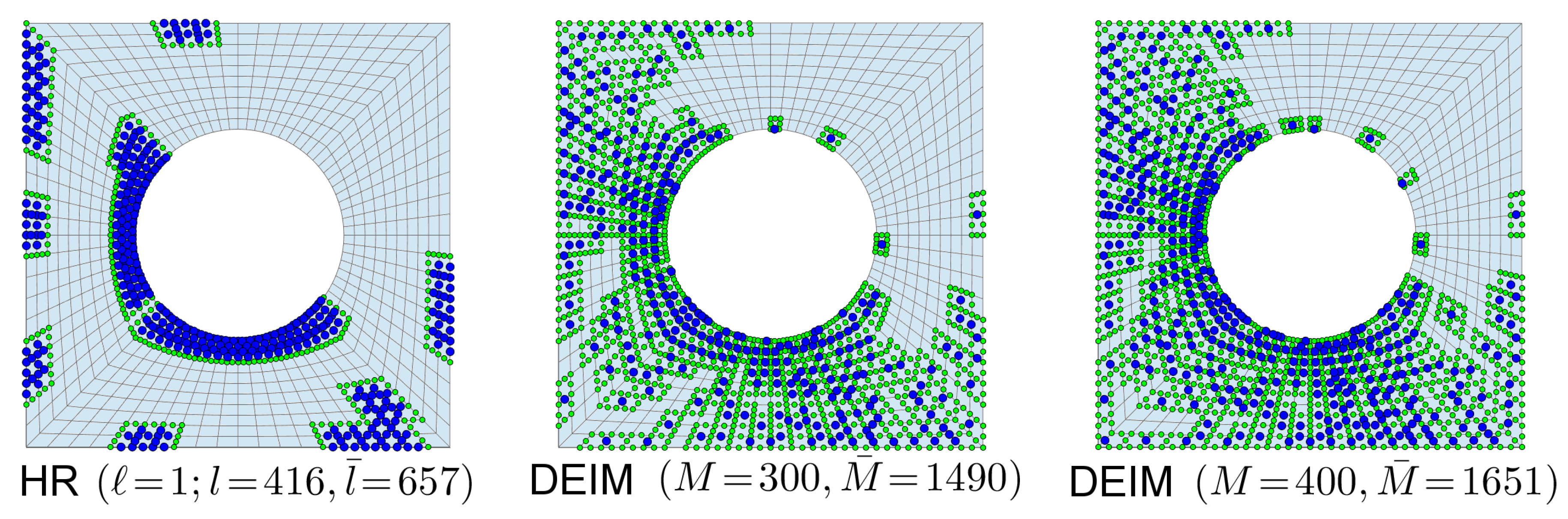
The offline procedure of the Hyper-Reduction method involves two steps. The first step is the construction of the Reduced Integration Domain ${\Omega }_Z$. For the present benchmark test, the RID is the union of a subdomain denoted by ${\Omega }^u$ generated from the reduced vector gradients ${(\nabla {\psi }_k)}_{k=1,\dots ,m}$, and a domain denoted by ${\Omega }^{+}$ corresponding to a set of neighboring elements to the previous subdomain. Usually, in the Hyper-reduction method, the user can select an additional subdomain of $\Omega$ in order to extend the RID over a region of interest. This subdomain is denoted by ${\Omega }_{user}$. In the sequel, to get small RIDs, ${\Omega }_{user}$ is empty. The set ${\Omega }^u$ consists of aggregated contributions ${\Omega }_k^u,k=1,\dots ,m$ from all the reduced vectors:

$$\begin{array}{cccc}\hfill {\Omega }_Z& :={\Omega }^u\cup {\Omega }^{+}\cup {\Omega }_{user},\hfill & \hfill {\Omega }^u& :={\cup }_{k=1}^m{\Omega }_k^u.\hfill \end{array}$$

(40)

To give the full details of the procedure, we introduce the domain partition in finite elements denoted ${({\Omega }_j^{\mathrm{e}}\subset \Omega )}_{j=1,\dots n_{\mathrm{el}}}$: $\Omega ={\cup }_{j=1}^{n_{\mathrm{el}}}{\Omega }_j^{\mathrm{e}}$, where $n_{\mathrm{el}}$ is the number of elements in the mesh. The domain ${\Omega }_k^u$ is the element where the maximum $L^2\left(\Omega \right)$ norm of the reduced vectors $\nabla {\tilde{\psi }}_k$ is reached. In [11], $\nabla {\tilde{\psi }}_k$ was set equal to $\nabla {\psi }_k$. Here, when applying the DEIM to ${(\nabla {\psi }_k)}_{k=1,\cdots ,m}$, the interpolation residuals provide a new reduced basis ${\left({\mathit{q}}_k\right)}_{k=1,\cdots ,m}$ (cf. Algorithm 6) related to temperature gradients. In this paper, $\nabla {\tilde{\psi }}_k$ is the output reduced basis produced by the DEIM, when it is applied to ${(\nabla {\psi }_k)}_{k=1,\cdots ,m}$. Other procedures, for the RID construction, are available in previous papers on hyper-reduction, e.g., [11,12]. The element selection reads for $k=1,\cdots ,m$:

$$\begin{array}{cc}\hfill {\Omega }_k^u& =\underset{{\Omega }_j^{\mathrm{e}},j=1,\cdots ,n_{\mathrm{el}}}{\arg \max }{∥\nabla {\tilde{\psi }}_k∥}_{L^2\left({\Omega }_j^{\mathrm{e}}\right)},\hfill \end{array}$$

(41)

where ${\parallel .\parallel }_{L^2\left({\Omega }_j^{\mathrm{e}}\right)}$ is the $L^2$ norm restricted to the element ${\Omega }_j^{\mathrm{e}}$. Several layers of surrounding elements denoted ${\Omega }^{+}$ can be added to ${\Omega }^u$.

The second step of the offline Hyper-Reduction procedure is the generation of truncated test functions that are zero outside of the RID. The truncation operator $P_Z$ is defined for all $u_h\in {\mathcal{V}}_0^{\mathrm{h}}$ by

$$\begin{array}{cc}\hfill P_Z\left(u_h\right)& :=\sum _{i\in \mathcal{F}}{\phi }_i{u}_{h,i},\mathcal{F}=\left\{i\in \{1,\cdots ,n\}|\underset{\Omega \setminus {\Omega }_Z}{\int }{\phi }_i{\phi }_i\mathrm{d}\Omega =0\right\}.\hfill \end{array}$$

(42)

Here, $\mathcal{F}$ is the set of indices of internal points, i.e., inner FE nodes, in ${\Omega }_Z$, which are related to the available FE equilibrium for predictions, which are forecasted only over ${\Omega }_Z$, i.e., for all $w\in {\mathcal{V}}_0^h$ holds with ${\Gamma }_2^Z:={\Gamma }_2\cap \partial {\Omega }_Z$

$$a(u_h,P_Z\left(w\right);\mathit{p})-l\left(P_Z\left(w\right)\right)=\underset{{\Omega }_Z}{\int }\mu (u_h;\mathit{p})\nabla u_h·\nabla \left(P_Z\left(w\right)\right)\mathrm{d}\Omega -\underset{{\Gamma }_2^Z}{\int }{P}_Z\left(w\right)q_{*}\mathrm{d}\Gamma .$$

(43)

The operator $P_Z$ can be represented by a truncated projector denoted Z. More precisely, if $\mathcal{F}=\{i_1,i_2,\dots ,i_l\}$ with $l:=\mathrm{card}\left(\mathcal{F}\right)$, then

$$\begin{array}{cccc}\hfill \mathit{Z}& :=[{\mathit{e}}_{i_1},{\mathit{e}}_{i_2},\dots ,{\mathit{e}}_{i_l}]\in {\mathbb{R}}^{n\times l},\hfill & \hfill P_Z\left(u_h\right)& :=\sum _{i=1}^n{\phi }_i{\left(\mathit{Z}{\mathit{Z}}^T\mathit{u}\right)}_i\hfill \end{array}$$

(44)

with ${\mathit{e}}_i\in {\mathbb{R}}^n$ the i-th unit vector. Therefore, the hyper-reduced form of the linearized prediction step is: for a given ${\mathbf{\gamma }}^{\left(\alpha \right)}$, find $\delta {\mathbf{\gamma }}^{\left(\alpha \right)}$ such that,

$$\begin{array}{cc}\hfill {\mathit{V}}^T\mathit{Z}{\mathit{Z}}^T\mathit{J}(\mathit{V}{\mathbf{\gamma }}^{\left(\alpha \right)};\mathit{p})\mathit{V}\delta {\mathbf{\gamma }}^{\left(\alpha \right)}& =-{\mathit{V}}^T\mathit{Z}{\mathit{Z}}^T\mathit{r}(\mathit{V}{\mathbf{\gamma }}^{\left(\alpha \right)};\mathit{p}),\hfill \end{array}$$

(45)

where J is given by (15) and ${\mathbf{\gamma }}^{(\alpha +1)}:={\mathbf{\gamma }}^{\left(\alpha \right)}+\delta {\mathbf{\gamma }}^{\left(\alpha \right)}$.

In addition to Z, we introduce also the operator $\overline{\mathit{Z}}\in {\mathbb{R}}^{n\times \overline{l}}$ that is a truncated projection operator onto the $\overline{l}$ points contained in the RID. In practice, the discrete unknowns are computed at these $\overline{l}\ge l$ points in order to compute the residual at the inner points l. Note that often $\overline{l}$ is significantly larger than l, especially if the RID consists of disconnected (scattered) regions.

The complexity of the products related to the fixed point operator J on the left-hand side term scale with $2\zeta lm+2l{m}^2$, where $\zeta$ is the maximum number of non-zero entries per row of J. For the right-hand side, the computational complexity is $2lm$. For both products, the complexity reduction factors are $n/l$. To obtain a well-posed hyper-reduced problem, one requires to fulfill the following condition $l\ge m$. If this condition is not fulfilled, the linear system of Equation (45) is rank deficient. In case of rank deficiency, one has to add more surrounding elements to the RID. The closer l to m, and the lower m, the less complex is the solution of the hyper-reduced formulation. The RID construction must generate a sufficiently large RID. If not, the convergence can be hampered, the number of correction steps can be increased and, moreover, the accuracy of the prediction can suffer. When ${\Omega }_Z=\Omega$, then Z is the identity matrix and the hyper-reduced formulation coincides with the usual system obtained by the Galerkin projection. An a posteriori error estimator for hyper-reduced approximations has recently been proposed in [31] for generalized standard materials.

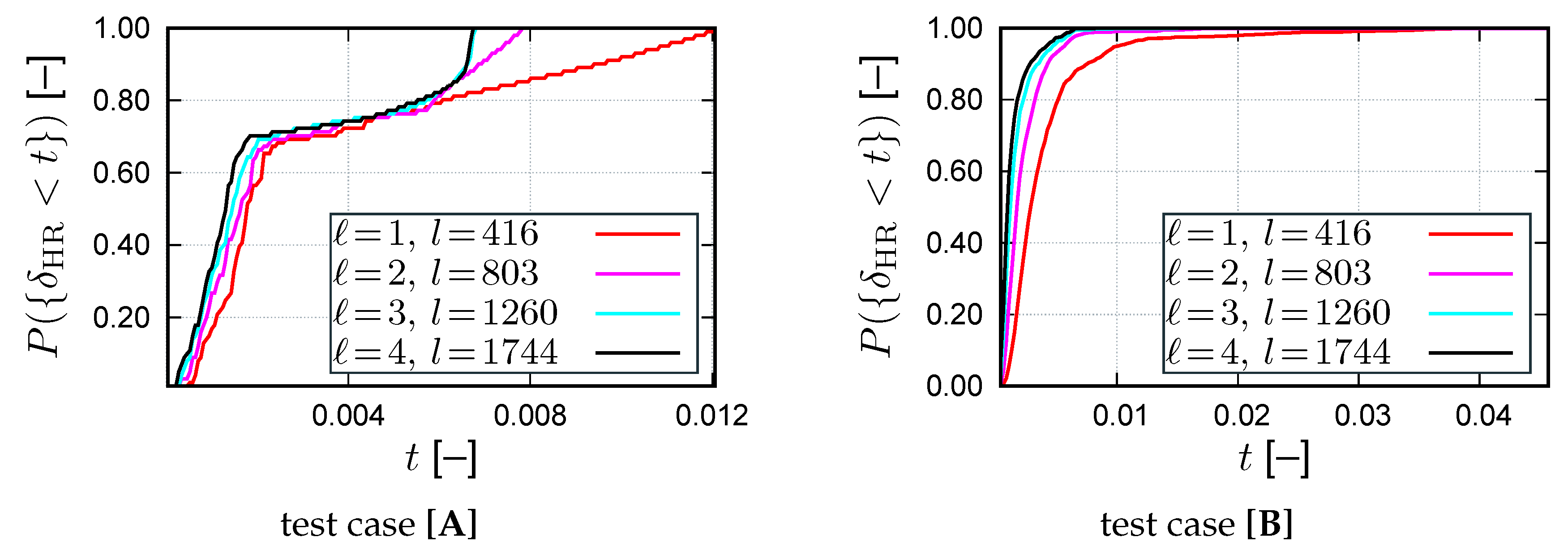
The offline phase of the hyper-reduction is summarized in Algorithm 6 and an algorithm of the online phase is provided in Algorithm 7.

3.4. Methodological Comparison

We comment on some formal commonalities and differences between the HR and the (D)EIM.

We first note that both methods reproduce the Galerkin–POD case, if $l=M=n$. For the HR, this means that the RID is the full domain, which implies that Z is a square permutation matrix, hence being invertible and yielding $\mathit{Z}{\mathit{Z}}^T=\mathit{I}$, thus (45) reduces to the POD–Galerkin reduced system (27). For the (D)EIM, this implies that the magic points consist of all grid points. We similarly obtain that P and U are invertible and thus $\mathit{U}{\left({\mathit{P}}^T\mathit{U}\right)}^{-1}{\mathit{P}}^T=\mathit{I}$ and (38) also reproduces the POD–Galerkin reduced system (27).

Algorithm 6: Offline Phase of the Hyper-Reduction (HR)

Algorithm 7: Online Phase of the Hyper-Reduction (HR)

Furthermore, we can state an equivalence of the DEIM and the HR under certain conditions, more precisely, the reduced system of the HR is a special case of the DEIM reduced system. Let us assume that the sampling matrices coincide and the collateral basis is also chosen as this sampling matrix, i.e., $\mathit{U}=\mathit{P}=\mathit{Z}$. Let us further assume that we have a Galerkin projection by choosing $\mathit{W}=\mathit{V}$ for the DEIM. Then, ${\mathit{P}}^T\mathit{U}={\mathit{Z}}^T\mathit{Z}={\mathit{I}}_M$ is the M-dimensional identity matrix, hence we obtain

$$\begin{array}{cc}\hfill \mathit{U}{\left({\mathit{P}}^T\mathit{U}\right)}^{-1}{\mathit{P}}^T& =\mathit{Z}{\left({\mathit{Z}}^T\mathit{Z}\right)}^{-1}{\mathit{Z}}^T=\mathit{Z}{\mathit{Z}}^T.\hfill \end{array}$$

(46)

Then, (38) yields

$$\begin{array}{cc}\hfill {\mathit{V}}^T\mathit{Z}{\mathit{Z}}^T\mathit{J}\mathit{V}\delta \mathbf{\gamma }& =-{\mathit{V}}^T\mathit{Z}{\mathit{Z}}^T\mathit{r},\hfill \end{array}$$

(47)

which is exactly the HR reduced system (45).

A common aspect of HR, and (D)EIM obviously is the point selection by a sampling matrix. The difference, however, is the selection criterion of the internal points. In case of the DEIM, these points are used as interpolation points, while, for the HR, they are used to specify the reduced integration domain.

A main difference of (D)EIM to HR is the way an additional collateral reduced-space is introduced in the reduced setting of the equations. The HR is more simple by not using an additional basis related to the residuals, but the implicit assumption, that $\mathrm{colspan}\left(\mathit{V}\right)$ (which approximates u) also approximates r and J well. This is a very reasonable assumption in symmetric elliptic problems and—in a certain way—it mimics the idea of having the same ansatz and test space as in any Galerkin formulation. However, from a mathematical point of view, it may not be valid in some more general cases, as in principle U and V are completely independent. For example, we can multiply the vectorial residual Equation (11) by an arbitrary regular matrix, hence arbitrarily change r (and thus U for the DEIM), but not changing u at all (i.e., not changing the POD-basis U). Hence, the collateral basis in the (D)EIM is first an additional technical ingredient and difficulty, which in turn allows for adopting the approximation space to the quantities that needs to be approximated well.

Theoretically, the EIM is well founded by analytical convergence results [32]. However, in addition, as a downside, the Lebesgue-constant, which essentially bounds the interpolation error to the best-approximation error, can grow exponentially. The DEIM is substantiated with a priori error estimates [10]. In particular, the error bounds depend on the conditioning of the small matrix ${\mathit{P}}^T\mathit{U}$. We are not aware of such a priori results for the HR, but also a posteriori error control has been presented in [31].

3.5. Computational Complexity

While the aim of model reduction is ultimately a reduction of the computing time, this quantity may heavily depend on the chosen implementation (see Section 4.6). Generally, the computational effort can be decomposed into the following contributions:

• the computation of the local unknowns and of their gradients $c_{\mathrm{reloc}}$ (gradient/temperature computation),
• the evaluations of the (nonlinear) constitutive model $c_{\mathrm{const}}$,
• the assembly of the residual $c_{\mathrm{rhs}}$ and of the Jacobian $c_{\mathrm{Jac}}$,
• the solution of the (dense) reduced linear system $c_{\mathrm{sol}}$.

From a theoretical point of view, the presented methods differ with respect to $c_{\mathrm{reloc}}$, $c_{\mathrm{const}}$, $c_{\mathrm{rhs}}$ and $c_{\mathrm{Jac}}$:

• Finite Element Simulation ($n_{\mathrm{gp}}$: number of integration points; $n_{\mathrm{el}}$: number of elements; $n_{\mathrm{el}}^{\mathrm{DOF}}$: degrees of freedom per element)

  $$\begin{array}{ccc}\hfill c_{\mathrm{reloc}}& =2n_{\mathrm{gp}}{n}_{\mathrm{el}}^{\mathrm{DOF}}\hfill & (\mathrm{gradient}/\mathrm{temperature}\mathrm{computation})\hfill \\ \hfill c_{\mathrm{const}}& \sim n_{\mathrm{gp}}\hfill & \left(\mathrm{constitutive}\mathrm{model}\right)\hfill \\ \hfill c_{\mathrm{rhs}}& =2n_{\mathrm{gp}}{n}_{\mathrm{el}}^{\mathrm{DOF}}\hfill & \left(\mathrm{residual}\mathrm{assembly}\right)\hfill \\ \hfill c_{\mathrm{Jac}}& =n_{\mathrm{gp}}\left[{\left(n_{\mathrm{el}}^{\mathrm{DOF}}\right)}^2+4n_{\mathrm{el}}^{\mathrm{DOF}}\right]\hfill & \left(\mathrm{Jacobian}\mathrm{assembly}\right)\hfill \\ \hfill c_{\mathrm{sol}}& \sim n^2.\hfill \end{array}$$
• Galerkin–POD

  $$\begin{array}{ccc}\hfill c_{\mathrm{reloc}}& =3n_{\mathrm{gp}}m\hfill & (\mathrm{gradient}/\mathrm{temperature}\mathrm{computation})\hfill \\ \hfill c_{\mathrm{const}}& \sim n_{\mathrm{gp}}\hfill & \left(\mathrm{constitutive}\mathrm{model}\right)\hfill \\ \hfill c_{\mathrm{rhs}}& =2m{n}_{\mathrm{gp}}\hfill & \left(\mathrm{direct}\mathrm{residual}\mathrm{assembly}\right)\hfill \\ \hfill c_{\mathrm{Jac}}& =(4m+m^2)n_{\mathrm{gp}}\hfill & \left(\mathrm{direct}\mathrm{Jacobian}\mathrm{assembly}\right)\hfill \\ \hfill c_{\mathrm{sol}}& \sim m^3.\hfill \end{array}$$
• Hyper-Reduction
  In the following, $n_{\mathrm{gp}}^{\mathrm{RID}}$ is the number of integration points in the RID. Furthermore, $c_{\mathrm{FE}}^{N,B}$ denotes the cost for the evaluation of u and $\nabla u$ using the FE matrices N and G and $c_{\mathrm{FE}}^r$ is the related to the cost for the residual computation on element level (both at least linear in the number of nodes per element + scattered assembly + overhead) and $c_{\mathrm{FE}}^K$ is the cost related to the contribution to the element stiffness at one element (∼number of nodes per element squared + scattered assembly + overhead). Lastly, $c_{\mathrm{A}}$ is the cost for the Jacobian assembly (i.e., matrix scatter operations).

  $$\begin{array}{ccc}\hfill c_{\mathrm{reloc}}& =\overline{l}m+n_{\mathrm{gp}}^{\mathrm{RID}}{c}_{\mathrm{FE}}^{N,B}\hfill & (\mathrm{get}u,{\partial }_{x}u,{\partial }_{y}u\mathrm{in}{\Omega }_Z)\hfill \\ \hfill c_{\mathrm{const}}& \sim n_{\mathrm{gp}}^{\mathrm{RID}}\hfill & \left(\mathrm{constitutive}\mathrm{model}\right)\hfill \\ \hfill c_{\mathrm{rhs}}& =n_{\mathrm{gp}}^{\mathrm{RID}}{c}_{\mathrm{FE}}^r+ml\hfill & \left(\mathrm{residual}\mathrm{assembly}\mathrm{and}\mathrm{projection}\right)\hfill \\ \hfill c_{\mathrm{Jac}}& =(m\omega +m^2)l+n_{\mathrm{gp}}^{\mathrm{RID}}{c}_{\mathrm{FE}}^K+c_{\mathrm{A}}\hfill & \left(\mathrm{Jacobian}\mathrm{assembly}\mathrm{and}\mathrm{projection}\right)\hfill \\ \hfill c_{\mathrm{sol}}& \sim m^3.\hfill \end{array}$$
• Discrete Empirical Interpolation Method
  The computational cost for the DEIM is closely related to the one of the HR by substituting M for l and $\overline{M}$ for $\overline{l}$ (denoting the number of nodes which are needed to evaluate the residual at the M magic points). Similar to the other methods, we denote $n_{\mathrm{gp}}^{\mathrm{DEIM}}$ as the number of quadrature points to evaluate the entries of the residual and Jacobian. In the cost notation of the Algorithm 5, we obtain

  $$\begin{array}{cc}\hfill c_{\mathrm{reloc}}& \sim m+nm\hfill \\ \hfill c_{\mathrm{const}}& =n_{\mathrm{gp}}^{\mathrm{DEIM}}\hfill & \left(\mathrm{constitutive}\mathrm{model}\right)\hfill \\ \hfill c_{\mathrm{rhs}}& \sim M\overline{M}\hfill & \left(\mathrm{residual}\mathrm{assembly}\mathrm{and}\mathrm{projection}\right)\hfill \\ \hfill c_{\mathrm{Jac}}& \sim M\overline{M}m\hfill & \left(\mathrm{Jacobian}\mathrm{assembly}\mathrm{and}\mathrm{projection}\right)\hfill \\ \hfill c_{\mathrm{sol}}& \sim m^3.\hfill \end{array}$$

From these considerations, the following conclusions can be drawn: First, the number of integration points ($n_{\mathrm{gp}}$, $n_{\mathrm{gp}}^{\mathrm{RID}}$, $n_{\mathrm{gp}}^{\mathrm{DEIM}}$) required for the residual and Jacobian evaluation enter linearly into the effort. Second, the reduced basis dimension m enters linearly into the residual assembly and both linearly and quadratically into the Jacobian assembly. Third, for the HR and the (D)EIM, the ratio $\overline{l}/l$ and $\overline{M}/M$ have a significant impact on the efficiency: for the considered 2D problem with quadratic ansatz functions, these ratios can range from 1 up to 21, i.e., for the same number of magic points pronounced variations in the runtime are in fact possible. The ratio $\overline{l}/l$ is determined by the topology of the RID, i.e., for connected RIDs it is smaller than for a scatter RID (i.e., for many disconnected regions forming the RID). Similarly, the (D)EIM has much smaller computational complexity in the case of magic points belonging to connected elements. Fourth, the Galerkin-POD can be based on simplified algebraic operations as no nodal variables need to be computed. This is due to the fact that the reduced residual and Jacobian are directly assembled without recurse to nodal coordinates and to any standard FE routine.

4. Numerical Results

4.1. ONLINE/OFFLINE Decomposition and RB Identification

In the following, we investigate the behavior of the heat conduction problem (1) for parameters, which we recall from Equation (7)

$$\begin{array}{cc}\hfill \mathit{p}& =[g_{\mathrm{x}},g_{\mathrm{y}},c,{\mu }_0,{\mu }_1]\in [0,1]\times [0,1]\times [1,2]\times \left\{1\right\}\times \left\{0.5\right\}.\hfill \end{array}$$

(48)

First, a regular parameter grid containing 125 equidistant snapshot points is generated and the high-fidelity FE model is solved for all those points yielding solutions $u_{h,i},i=1,\dots ,125$. Here, the FEM discretization is based on a discretization into 800 biquadratic quadrilateral elements comprising a total of 2560 nodes (including 160 boundary nodes). The problem hence has $n=2400$ unknowns. In order to exemplify the nonlinearity of the problem due to the temperature dependent conductivity, the conductivity (top row) and the temperature field (bottom row) are shown for three different parameters in Figure 2.

Then, a snapshot POD is performed in order to obtain an RB from the snapshots, and the normalized spectrum of the snapshot correlation matrix is shown in Figure 3. Different dimensions of the RB are considered with the projection error

$$\begin{array}{cc}\hfill E_m& =\sqrt{\frac{{\sum }_{i=1}^{125}{\parallel u_h\left({\mathit{p}}_i\right)-{\tilde{P}}_m{u}_h\left({\mathit{p}}_i\right)\parallel }_{L^2\left(\Omega \right)}^2}{{\sum }_{i=1}^{125}{\parallel u_h\left({\mathit{p}}_i\right)\parallel }_{L^2\left(\Omega \right)}^2}}\hfill \end{array}$$

(49)

given in

Table 1. Dimension of the RB vs. projection error for the snapshots.

Dimension of RB	16	24	32	48	60
$E_m$	6.629 × 10−3	4.120 × 10−3	3.180 × 10−3	2.017 × 10−3	1.486 × 10−3

and the decay is visualized in Figure 3 (right). Here, ${\tilde{P}}_m$ denotes the orthogonal projection operator onto the m-dimensional RB with respect to the standard inner product ${\langle ·,·\rangle }_{L^2\left(\Omega \right)}$ in the $L^2\left(\Omega \right)$ function space

$$\begin{array}{cccc}\hfill {\tilde{P}}_m{u}_h\left(\mathit{p}\right)& =\sum _{i=1}^m\sum _{k=1}^m{\psi }_i{\left({\tilde{\mathit{M}}}^{-1}\right)}_{ik}{〈u_h\left(\mathit{p}\right),{\psi }_k〉}_{L^2\left(\Omega \right)},\hfill & \hfill {\tilde{M}}_{ik}& ={〈{\psi }_i,{\psi }_k〉}_{L^2\left(\Omega \right)}i,j=1,\cdots ,m.\hfill \end{array}$$

(50)

The low approximation errors $E_m$ given in Table 1 and in Figure 3 (right) indicate that the training data can essentially be represented rather accurately by the RB using a projection. Additionally, the projection error naturally decreases with increasing dimension. However, the solution of the reduced problem does not necessarily follow the same monotonicity. Since $\mu$ is bounded away from 0 due to ${\mu }_0>0$, the problem under consideration is coercive. Similar to the linear case, we expect that the approximation error $e\left(\mathit{p}\right)=\tilde{w}(\mathbf{\gamma }\left(\mathit{p}\right);\mathit{p})-w_h\left(\mathit{p}\right)$ and the projection error are comparable in the sense that

$$\begin{array}{c}\hfill \eta \left(\mathit{p}\right):=\frac{{\parallel e\left(\mathit{p}\right)\parallel }_{L^2\left(\Omega \right)}}{\parallel u_h-{\tilde{P}}_m{u}_h{\parallel }_{L^2\left(\Omega \right)}}\end{array}$$

(51)

is small. Due to the best-approximation by the orthogonal projection, we certainly have $\eta \left(\mathit{p}\right)\ge 1$. Numerical Values are provided in the following. The constant $\eta \left(\mathit{p}\right)$ is generally not available in closed form for the considered nonlinear problem. Assuming a constant conductivity $\mu$ evaluated at the solution $u\left(\mathit{p}\right)$, an upper bound ${\eta }_{\mathrm{UB}}\left(\mathit{p}\right)$ for the numerically determined $\eta \left(\mathit{p}\right)$ is provided via Cea’s Lemma (for symmetric problems):

$$\begin{array}{cccccc}\hfill {\eta }_{\mathrm{UB}}^{\mathrm{h}}& :=\sqrt{\frac{{\widehat{c}}_{\mathrm{h}}\left(\mathit{p}\right)}{{\check{c}}_{\mathrm{h}}\left(\mathit{p}\right)}},\hfill & \hfill {\widehat{c}}_{\mathrm{h}}& :=\underset{v_{\mathrm{h}},w_{\mathrm{h}}\in {\mathcal{V}}_0^{\mathrm{h}}\setminus \left\{0\right\}}{\sup }\frac{a_{\mathrm{c}}(v_{\mathrm{h}},w_{\mathrm{h}};\mathit{p})}{\parallel v_{\mathrm{h}}{\parallel }_{L^2\left(\Omega \right)}{\parallel w_{\mathrm{h}}\parallel }_{L^2\left(\Omega \right)}},\hfill & \hfill {\check{c}}_{\mathrm{h}}& :=\underset{v_{\mathrm{h}}\in {\mathcal{V}}_0^{\mathrm{h}}\setminus \left\{0\right\}}{\inf }\frac{a_{\mathrm{c}}(v_{\mathrm{h}},v_{\mathrm{h}};\mathit{p})}{\parallel v_{\mathrm{h}}{\parallel }_{L^2\left(\Omega \right)}^2}.\hfill \end{array}$$

(52)

Here, ${\widehat{c}}_{\mathrm{h}}$ and ${\check{c}}_{\mathrm{h}}$ are the continuity constant and the coercivity constant of the condensed bilinear form

$$\begin{array}{c}\hfill a_{\mathrm{c}}(w_{\mathrm{h}},v_{\mathrm{h}};\mathit{p}):=\underset{\Omega }{\int }\nabla w_{\mathrm{h}}·\mu (u_{\mathrm{h}}\left(\mathit{p}\right);\mathit{p})\nabla v_h\mathrm{d}\Omega (\forall v_{\mathrm{h}},w_{\mathrm{h}}\in {\mathcal{V}}_0^{\mathrm{h}}),\end{array}$$

(53)

with $u_{\mathrm{h}}\left(\mathit{p}\right)$ denoting the Finite Element solution of the nonlinear problem. The estimate ${\eta }_{\mathrm{UB}}^{\mathrm{h}}$ is not a tight bound and, at the same time, its numerical evaluation is computationally expensive, so it is typically considered to be of limited practical use.

4.2. Test Cases

In order to investigate the accuracy of the reduced models, additional parameter vectors need to be considered that are not matching the training data. Two test cases are considered in the sequel:

[A] 

A diagonal in the parameter space is considered with

$$\begin{array}{cccccc}\hfill {\mathit{p}}^{\left(j\right)}& :={\mathit{p}}_0+{\beta }^{\left(j\right)}(\widehat{\mathit{p}}-{\mathit{p}}_0),\hfill & \hfill {\mathit{p}}_0& :=[0,0,1,1,1/2],\hfill & \hfill \widehat{\mathit{p}}& :=[1,1,2,1,1/2].\hfill \end{array}$$

(54)

A total of 101 equally spaced values of ${\beta }^{\left(j\right)}$ was chosen, i.e., ${\beta }^{\left(j\right)}=\frac{j}{100}$ for $j=0,1,\cdots ,100$.

[B] 

A set of 1000 random parameters ${\mathit{p}}^{\left(j\right)}$ was generated using a uniform distribution in parameter space, i.e., a uniform distribution $\mathcal{U}\left(\right[0,1\left]\right)$ was chosen for $g_{\mathrm{x}}$, $g_{\mathrm{y}}$ and the parameter c was assumed to be distributed via $\mathcal{U}\left(\right[1,2\left]\right)$.

4.3. Certification of the Galerkin RB Method

First, the ability of the Galerkin RB solution to approximate the optimal orthogonal projection and, thereby, the high-fidelity solution, was verified. Therefore, the constant $\eta \left(\mathit{p}\right)$ was evaluated for all snapshots of case [A] and [B]. The minimum, the mean and the maximum of $\eta \left(\mathit{p}\right)$ were determined for the 101 and 1000 test of case [A] and [B], respectively. The results shown in

Table 2. Computed values of $\eta \left(\mathit{p}\right)$ for different modes sets and for test cases [A], [B]; the last row represents the upper bound ${\eta }_{\mathrm{UB}}^{\mathrm{h}}\ge \eta \left(\mathit{p}\right)$.

Test Case	[A]			[B]
	min.	mean	max.	min.	mean	max.
$m=16$	1.000	1.4708	1.8248	1.000	1.3185	2.0239
$m=24$	1.000	1.9088	2.8926	1.000	1.3187	2.6559
$m=32$	1.000	1.7273	2.7441	1.000	1.3679	2.4393
$m=48$	1.000	1.5386	2.0232	1.000	1.3051	1.9371
$m=60$	1.000	1.5096	1.9333	1.000	1.3447	1.8922
${\eta }_{\mathrm{UB}}^{\mathrm{h}}$ cf. (52)	62.12	64.693	70.581	62.51	74.728	82.504

state the POD approximation error is found close to the projection error. This confirms the quality of the chosen RB.

Note that in test case [B] only a finite number of random parameter vectors was chosen which does not necessarily contain the extreme values of $\eta \left(\mathit{p}\right)$. The numerical data in Table 2 for test case [A] shows that indeed, [A] contains parameters leading to larger values of $\eta \left(\mathit{p}\right)$. When increasing the size of the random parameter set for [B], the maximum values of $\eta \left(\mathit{p}\right)$ in case [B] should be equal or larger than the maximum values of case [A].

In addition to the error magnification parameter $\eta \left(\mathit{p}\right)$, the minimum, average and maximum of the relative error

$$\begin{array}{cc}\hfill \delta (\tilde{u}\left(\mathit{p}\right),\mathit{p})& =\frac{\parallel \tilde{u}\left(\mathit{p}\right)-u_h{\left(\mathit{p}\right)\parallel }_{L^2\left(\Omega \right)}}{\parallel u_h{\left(\mathit{p}\right)\parallel }_{L^2\left(\Omega \right)}}\hfill \end{array}$$

(55)

are also computed for all samples. The results are provided in

Table 3. Relative error of the Galerkin RB approximation.

Test Case	[A]			[B]
	min.	mean	max.	min.	mean	max.
$m=16$	0.00   10−3	2.54   10−3	7.28   10−3	0.67   10−3	1.75   10−3	7.49  10−3
$m=24$	0.00   10−3	1.07   10−3	3.80   10−3	0.16   10−3	0.88   10−3	5.29  10−3
$m=32$	0.00   10−3	0.82   10−3	3.23  10−3	0.18   10−3	0.63   10−3	3.13  10−3
$m=48$	0.00   10−3	0.31   10−3	1.14  10−3	0.06   10−3	0.33   10−3	2.07  10−3
$m=60$	0.00  10−3	0.20   10−3	0.70  10−3	0.05   10−3	0.26   10−3	1.55  10−3

. Note that for test case [A] the minimum error is truly zero for $g_{\mathrm{x}}=g_{\mathrm{y}}=0$, which implies a homogeneous zero temperature. For an RB of dimension 32, the mean error is well below 10⁻³ for all tests and the maximum error over all tests is 3.23 × 10⁻³. This basis provides a compromise between accuracy and computational cost and is therefore used for the comparison of the methods in the sequel.

Note that the slow decay of the accuracy of the Galerkin approximation indicated by the data provided in Table 3 indicates that the information content captured in the training snapshots is not sufficient to provide better accuracies. Therefore, we decided on a dimension $m=32$ for the reduced basis in the subsequent experiments.

In order to further reduce the computational cost, the use of additional reduction techniques such as the Hyper-Reduction (HR) and Discrete Empirical Interpolation Method (DEIM) is required. Note also that the reduction techniques using a POD basis are only approximations of the Galerkin RB. Hence, the HR and DEIM cannot be better than the Galerkin RB solution except in few cases where ${\eta }_{\mathrm{HR}}\left(\mathit{p}\right)<\eta \left(\mathit{p}\right)$ or ${\eta }_{\mathrm{DEIM}}\left(\mathit{p}\right)<\eta \left(\mathit{p}\right)$, where ${\eta }_{\mathrm{HR}}\left(\mathit{p}\right)$ and ${\eta }_{\mathrm{DEIM}}\left(\mathit{p}\right)$ denote the constant $\eta$ from (51) for the HR and DEIM method. In our numerical tests, this occurred only exceptionally, which can be explained by the slightly different considered residual in comparison to the Galerkin RB. Let us now turn to a more realistic multi-query situation where RB is crucial for non-prohibitive runtimes.

4.4. Application to Uncertainty Quantification

In real world simulation scenarios, material coefficients and boundary conditions are often not exactly known and one is interested in the impact of this uncertainty on the quantities of interest. To this end, uncertainty quantification (UQ) has been proposed and has become an active research field on its own. In classical forward UQ, the critical parameters are modeled as random variables; the distributions and correlation are derived from measurements as for example shown for nonlinear material curves in [33]. Finally, the forward model is evaluated at collocation points ${\mathit{p}}_i$ in the parameter space according to a quadrature method as e.g., Monte Carlo, [34]. Typically, many collocations (or ‘sampling’) points are needed and therefore model order reduction has been shown to significantly reduce the computational costs, e.g., [35].

In the case of our thermal benchmark problem, the parameter vector $\mathit{p}=\mathit{P}\left(\omega \right)$ is considered as a realization of the random vector, where $\omega \in {\Omega }_{\mathrm{p}}$ and $({\Omega }_{\mathrm{p}},\mathcal{F},\mathcal{P})$ is the usual probability space. We refer to this as test case [C] and assume that the random variables are independent and uniformly distributed as already introduced in test case [B]

$$\begin{array}{cc}\hfill \mathit{P}\left(\omega \right)& =[G_{\mathrm{x}}\left(\omega \right),G_{\mathrm{y}}\left(\omega \right),C\left(\omega \right)]\mathrm{with}{G}_{\mathrm{x}},G_{\mathrm{y}}\sim \mathcal{U}\left([0,1]\right)\mathrm{and}C\sim \mathcal{U}\left([1,2]\right).\hfill \end{array}$$

Finally, the statistical moments of the solution $u_{\star }(x;P\left(\omega \right))$ are approximated by the Monte Carlo method, e.g., [34]

$$\begin{array}{cc}\hfill \mathbb{E}\left(u_{\star }(\mathit{x};\mathit{P})\right)& \approx \frac{1}{n_{\mathrm{p}}}\sum _{j=1}^{n_{\mathrm{p}}}{u}_{\star }(\mathit{x};{\mathit{p}}^{\left(j\right)})=:{\overline{u}}_{\star }\left(\mathit{x}\right),\hfill \end{array}$$

(56)

$$\begin{array}{cc}\hfill {\mathbb{M}}^k\left(u_{\star }(\mathit{x};\mathit{P})\right)& \approx \frac{1}{n_{\mathrm{p}}}\sum _{j=1}^{n_{\mathrm{p}}}{\left(u_{\star }(\mathit{x};{\mathit{p}}^{\left(j\right)})-{\overline{u}}_{\star }\left(\mathit{x}\right)\right)}^k=:m_{\star }^k\left(\mathit{x}\right),\hfill \end{array}$$

(57)

where ${\mathit{p}}^{\left(j\right)}$ are the same $n_{\mathrm{p}}=1000$ random sample points generated for case [B] and $u_{\star }$ and $m_{\star }^k$ are the approximations of the solution and its k-th centered moment ($k>1$) obtained from Finite Elements, Galerkin RB, DEIM and HR, i.e., $\star \in \{\mathrm{h},\mathrm{RB},\mathrm{DEIM},\mathrm{HR}\}$, respectively (e.g., $m_{\mathrm{h}}^3$ is the third statistical moment obtained from Finite Element computations). For the DEIM, we selected a fixed number of $M=400$ magic points, which is a conservative choice (see Figure 4 for a discussion). In practice, one may choose an adaptive selection strategy.

An estimation of the normalized root mean square error of the finite element solution due to Monte Carlo sampling can be obtained by

$$\begin{array}{cc}\hfill E_{\mathrm{MC}}& =\frac{1}{\sqrt{n_{\mathrm{p}}}{\parallel {\overline{u}}_{\mathrm{FE}}\parallel }_{L^2\left(\Omega \right)}}{∥\sqrt{m_h^2}∥}_{L^2\left(\Omega \right)}\approx 1.78·{10}^{-2}\equiv 1.78\%.\hfill \end{array}$$

This implies that the accuracy of the reduced models in the prediction of ${\overline{u}}_{\star }$ should be around 2% or better, in order to render the reduced models capable of providing meaningful quantitative statistical information. Figure 5 shows the error in the moments computed for the various reduction techniques with respect to the finite element reference solution

$$\begin{array}{cc}\hfill E_{\star }^k& =\frac{\parallel m_{\star }^k-m_h^k{\parallel }_{L^2\left(\Omega \right)}}{\parallel m_h^k{\parallel }_{L^2\left(\Omega \right)}}.\hfill \end{array}$$

The figure indicates that the approximations of the expected value ${\overline{u}}_{\star }$ are at least accurate up to ${10}^{-3}$ and thus below (i.e., better than) the sampling accuracy $E_{\mathrm{MC}}$. Generally, the DEIM tends to perform better than the HR; the largest errors occur for $E_{\mathrm{HR}}^7=1.09\times {10}^{-1}$ and $E_{\mathrm{DEIM}}^7=3.46\times {10}^{-2}$, respectively.

4.5. Accuracy of the HR and DEIM vs. Number of Interpolation Points

Both the HR and the DEIM sample the nonlinearity only at entries on the right-hand side: the interpolation points. The HR has one additional parameter ℓ describing how many element layers around a certain degree of freedom (DOF) should be considered in order to generate ${\Omega }^{+}$, which add additional interpolation points to the RID. The location of the DOF around which the interpolation points are located are selected based on the criterion described in Section 3.3. In contrast to that, the DEIM selects the points using only the right-hand side information of the system. For the DEIM, the number of sampling points M is an input parameter describing the dimension of the collateral basis. The effect of the number of points is investigated in the following. Based on the considerations in Section 3.4, both the HR and the DEIM should reproduce the POD solution for a large number of sampling sites, while, for a lower number of points, the accuracy is a trade-in for computational efficiency.

For the DEIM, different interpolation point numbers are considered for both test cases [A] and [B]. The resulting relative errors are compared in Figure 4 in terms of the statistical distribution function $P\left(t\right)$ of the relative error, i.e., the probability of finding a relative error $\delta$ that is smaller than or equal to t. Obviously the number of interpolation points has a pronounced impact on the distribution. Generally, the error function for a low number of points states a significant increase of the computational error due to DEIM in comparison with the POD. With an increasing number of points, the distribution function approaches the one of the POD. In our test, the use of more than 300 sampling points can only improve the accuracy in a minor way. We must note that, in general, the accuracy of the DEIM must not be a monotonic function of interpolation points number.

For the hyper-reduced predictions, different layers of elements are added in ${\Omega }^{+}$ in order to extend the RID. We have considered here $\ell =$ 1, 2, 3 and 4 layers of elements connected to ${\Omega }^u$, for both test cases [A] and [B]. The resulting relative errors are compared in Figure 6 in terms of the statistical distribution function $P\left(t\right)$ of the relative error. With increasing number of layers, the distribution function approaches the one of the POD. The number of internal points, l, increases rapidly when increasing the number of layers. In the case of the DEIM, the growth of interpolation points is much more progressive. More than two layers of elements do not improve the accuracy significantly.

One layer of additional elements gives predictions less accurate than the DEIM for approximately the same number of internal points/interpolation points (here: $l=416$ for the HR and $M=300$ for the DEIM). However, the number of additional points required for the residual evaluation differs considerably: $\overline{l}=657$ vs. $\overline{M}=1490$. This can be explained by direct comparison of the reduced domains in Figure 7. For the Hyper-reduction, the RID is rather compact (leftmost plot) while the magic points of the DEIM are rather scattered, thus requiring the temperature evaluation at many additional points.

The predictions of the Hyper-reduction are particularly less accurate, which can especially be seen by comparing Figure 4 (left, test case [A], black line) and Figure 6 (left, test case [A], red line), where 80% of the samples lead to errors below $\approx 0.002$ for the DEIM and $\approx 0.01$ for the HR. Nevertheless, the accuracy of the hyper-reduced predictions is generally of the same order of magnitude as the accuracy of the DEIM.

4.6. Computing Times

Although the main objective of model reduction is the reduction of computing time, this paper does not aim at benchmarking HR and DEIM. If not optimized properly, runtime benchmarks compare rather the performance of the implementations than that of the algorithms. Nonetheless, the numbers in

Table 4. Elapsed time and number of failures of the nonlinear solver for the solution of all computations of test case [A] (101 solves) and [B] (1000 solves) for Finite Element (FE), Hyper-Reduction (HR) with varying number of additional element layers $\ell \in \{1,2,3,4\}$, DEIM for $M\in \{200,250,300,400\}$ magic points; all computations are carried out using $N=32$ POD modes.

	Test Case [A]		Test Case [B]
	Time	Fail	Time	Fail
FE	59.9 s	-	660.5	-
HR, $\ell =1$	10.6 s	0	118.9 s	5
HR, $\ell =2$	17.4 s	0	180.6 s	2
HR, $\ell =3$	24.5 s	0	247.2 s	1
HR, $\ell =4$	30.9 s	0	303.5 s	0
DEIM, $M=200$	20.6 s	0	292.3 s	108
DEIM, $M=250$	21.4 s	0	240.6 s	7
DEIM, $M=300$	24.4 s	0	249.0 s	3
DEIM, $M=400$	27.6 s	0	272.7 s	2

indicate the effect of varying parameters in the respective techniques using our Matlab implementation. In the case of a few magic points, divergence of the fixed point iteration was observed for a small number of configurations in the parametric space. The number is stated in the table as failure. HR and DEIM have similar performance, although HR seems to be slightly more robust for the problem at hand in the sense that it exhibits slightly less failures of the iterative solver. Finally, as expected, the overall runtime scales linearly with the number of solves, i.e., computing test case [B] is approx. 10 times slower than [A].

5. Conclusions

The presented study revisits an—at first sight—rather simple nonlinear heat conduction problem. In order to accelerate the nonlinear computations, a Galerkin reduced basis ansatz is proposed (see Section 3.1) using preliminary offline computations in the established framework of the snapshot POD.

Both the HR and the (D)EIM can achieve significant accelerations of the computing time. These scale approximately with the number of magic points (here: l or M) and/or with the number of points connected to the magic points ($\overline{l}$ and $\overline{M}$, respectively). In the presented examples, less than 25% of the original mesh were considered in both the (D)EIM and the HR. By virtue of the considerations presented in Section 3.5, the computing times are reduced accordingly.

The selection of the magic points in the HR and the (D)EIM requires the computation of the solution at an increased number of nodes, i.e., $\overline{l}\ge l$ and $\overline{M}\ge M$, respectively. The higher the space dimension (2D, 3D, ...), the more scattered the magic points and the higher the number of degrees of freedom per element, the more are $\overline{l}$ and $\overline{M}$ increased in comparison to l and M.

With respect to the implementation, it shall be noted that the HR is less intrusive than the (D)EIM as it uses standard simulation outputs to generate the modes, while the (D)EIM requires additional outputs for the construction of the collateral basis. Other than that, both techniques can be implemented using mostly the same implementation, which is also confirmed by the similarity of both techniques presented in Section 3.4.

References

1. Gubisch, M.; Volkwein, S. POD for Linear-Quadratic Optimal Control. In Model Reduction and Approximation: Theory and Algorithms; Benner, P., Cohen, A., Ohlberger, M., Willcox, K., Eds.; SIAM: Philadelphia, PA, USA, 2017. [Google Scholar]
2. Volkwein, S. Optimal control of a phase-field model using proper orthogonal decomposition. ZAMM 2001, 81, 83–97. [Google Scholar] [CrossRef]
3. Antoulas, A. Approximation of Large–Scale Dynamical Systems; SIAM Publications: Philadelphia, PA, USA, 2005. [Google Scholar]
4. Patera, A.; Rozza, G. Reduced Basis Approximation and a Posteriori Error Estimation for Parametrized Partial Differential Equations; Version 1.0, Copyright MIT 2006-2007, to Appear in (Tentative Rubric) MIT Pappalardo Graduate Monographs in Mechanical Engineering; Massachusetts Institute of Technology (MIT): Cambridge, MA, USA, 2007. [Google Scholar]
5. Haasdonk, B. Reduced Basis Methods for Parametrized PDEs—A Tutorial Introduction for Stationary and Instationary Problems. In Model Reduction and Approximation: Theory and Algorithms; Benner, P., Cohen, A., Ohlberger, M., Willcox, K., Eds.; SIAM: Philadelphia, PA, USA, 2017. [Google Scholar]
6. Barrault, M.; Maday, Y.; Nguyen, N.; Patera, A. An ’empirical interpolation’ method: Application to efficient reduced-basis discretization of partial differential equations. C. R. Math. Acad. Sci. Paris Ser. I 2004, 339, 667–672. [Google Scholar] [CrossRef]
7. Haasdonk, B.; Ohlberger, M. Reduced basis method for explicit finite volume approximations of nonlinear conservation laws. In Proceedings of the HYP 2008, International Conference on Hyperbolic Problems: Theory, Numerics and Applications, Providence, RI, USA, 9–13 June 2008; American Mathematical Society: Providence, RI, USA, 2009; Volume 67, pp. 605–614. [Google Scholar]
8. Drohmann, M.; Haasdonk, B.; Ohlberger, M. Reduced Basis Approximation for Nonlinear Parametrized Evolution Equations based on Empirical Operator Interpolation. SIAM J. Sci. Comput. 2012, 34, A937–A969. [Google Scholar] [CrossRef]
9. Chaturantabut, S.; Sorensen, D.C. Discrete empirical interpolation for nonlinear model reduction. In Proceedings of the 48th IEEE Conference on Decision and Control and the 28th Chinese Control Conference (CDC/CCC 2009), Shanghai, China, 15–18 December 2009; pp. 4316–4321. [Google Scholar]
10. Chaturantabut, S.; Sorensen, D.C. A State Space Error Estimate for POD-DEIM Nonlinear Model Reduction. SIAM J. Numer. Anal. 2012, 50, 46–63. [Google Scholar] [CrossRef]
11. Ryckelynck, D. A priori hypereduction method: An adaptive approach. J. Comput. Phys. 2005, 202, 346–366. [Google Scholar] [CrossRef]
12. Ryckelynck, D. Hyper reduction of mechanical models involving internal variables. Int. J. Numer. Methods Eng. 2009, 77, 75–89. [Google Scholar] [CrossRef]
13. Everson, R.; Sirovich, L. Karhunen-Loève procedure for gappy data. J. Opt. Soc. Am. A 1995, 12, 1657–1664. [Google Scholar] [CrossRef]
14. Astrid, P.; Weiland, S.; Willcox, K.; Backx, T. Missing point estimation in models described by proper orthogonal decomposition. IEEE Trans. Autom. Control 2008, 53, 2237–2251. [Google Scholar] [CrossRef]
15. Carlberg, K.; Bou-Mosleh, C.; Farhat, C. Efficient non-linear model reduction via a least-squares Petrov–Galerkin projection and compressive tensor approximations. Int. J. Numer. Methods Eng. 2011, 86, 155–181. [Google Scholar] [CrossRef]
16. Farhat, C.; Avery, P.; Chapman, T.; Cortial, J. Dimensional reduction of nonlinear finite element dynamic models with finite rotations and energy-based mesh sampling and weighting for computational efficiency. Int. J. Numer. Methods Eng. 2014, 98, 625–662. [Google Scholar] [CrossRef]
17. Fritzen, F.; Hodapp, M. The Finite Element Square Reduced (FE2R) method with GPU acceleration: Towards three-dimensional two-scale simulations. Int. J. Numer. Methods Eng. 2016, 107, 853–881. [Google Scholar] [CrossRef]
18. Fritzen, F.; Xia, L.; Leuschner, M.; Breitkopf, P. Topology optimization of multiscale elastoviscoplastic structures. Int. J. Numer. Methods Eng. 2016, 106, 430–453. [Google Scholar] [CrossRef]
19. Dimitriu, G.; Ştefănescu, R.; Navon, I.M. Comparative numerical analysis using reduced-order modeling strategies for nonlinear large-scale systems. J. Comput. Appl. Math. 2017, 310, 32–43. [Google Scholar] [CrossRef]
20. Bathe, K.I. Finite-Elemente-Methoden; Springer: Berlin/Heidelberg, Germany, 2002. [Google Scholar]
21. Zienkiewicz, O.; Taylor, R.; Zhu, J. Finite Element Method; Butterworth-Heinemann: Oxford, UK, 2006. [Google Scholar]
22. Kelley, C.T. Iterative Methods for Linear and Nonlinear Equations; SIAM: Philadelphia, PA, USA, 1995. [Google Scholar]
23. Sirovich, L. Turbulence and the dynamics of coherent structures part I: Coherent structures. Q. Appl. Math. 1987, 65, 561–571. [Google Scholar] [CrossRef]
24. Joliffe, I. Principal Component Analysis; John Wiley & Sons: Hoboken, NJ, USA, 2002. [Google Scholar]
25. Ştefănescu, R.; Sandu, A.; Navon, I.M. Comparison of POD reduced order strategies for the nonlinear 2D shallow water equations. Int. J. Numer. Methods Fluids 2014, 76, 497–521. [Google Scholar] [CrossRef]
26. Fritzen, F.; Hodapp, M.; Leuschner, M. GPU accelerated computational homogenization based on a variational approach in a reduced basis framework. Comput. Methods Appl. Mech. Eng. 2014, 278, 186–217. [Google Scholar] [CrossRef]
27. Haasdonk, B.; Ohlberger, M.; Rozza, G. A Reduced Basis Method for Evolution Schemes with Parameter-Dependent Explicit Operators. ETNA Electron. Trans. Numer. Anal. 2008, 32, 145–161. [Google Scholar]
28. Wirtz, D.; Sorensen, D.; Haasdonk, B. A Posteriori Error Estimation for DEIM Reduced Nonlinear Dynamical Systems. SIAM J. Sci. Comput. 2014, 36, A311–A338. [Google Scholar] [CrossRef]
29. Ryckelynck, D.; Missoum Benziane, D. Multi-level a priori hyper reduction of mechanical models involving internal variables. Comput. Methods Appl. Mech. Eng. 2010, 199, 1134–1142. [Google Scholar] [CrossRef] [Green Version]
30. Ryckelynck, D.; Vincent, F.; Cantournet, S. Multidimensional a priori hyper-reduction of mechanical models involving internal variables. Comput. Methods Appl. Mech. Eng. 2012, 225, 28–43. [Google Scholar] [CrossRef]
31. Ryckelynck, D.; Gallimard, L.; Jules, S. Estimation of the validity domain of hyper-reduction approximations in generalized standard elastoviscoplasticity. Adv. Model. Simul. Eng. Sci. 2015, 2, 6. [Google Scholar] [CrossRef]
32. Maday, Y.; Nguyen, N.; Patera, A.; Pau, G. A General, Multi-Purpose Interpolation Procedure: The Magic Points; Technical Report RO7037; Laboratoire Jaques-Louis-Lions, Université Piere et Marie Curie: Paris, France, 2007. [Google Scholar]
33. Römer, U.; Schöps, S.; Weiland, T. Stochastic Modeling and Regularity of the Nonlinear Elliptic curl-curl Equation. SIAM/ASA J. Uncertain. Quantif. 2016, 4, 952–979. [Google Scholar] [CrossRef]
34. Xiu, D. Numerical Methods for Stochastic Computations: A Spectral Method Approach; Princeton University Press: Princeton, NI, USA, 2010. [Google Scholar]
35. Haasdonk, B.; Urban, K.; Wieland, B. Reduced Basis Methods for parameterized partial differential equations with stochastic influences using the Karhunen-Loeve expansion. SIAM/ASA J. Uncertain. Quantif. 2013, 1, 79–105. [Google Scholar] [CrossRef]
Figure 1. Geometry of the planar benchmark problem (left) and nonlinearity of the temperature dependent conductivity μ (right).
Mca 23 00008 g001
Figure 2. Parameter dependent conductivity μ ( u ; p ) (top row) and solution u ( x ; p ) (bottom row) for three different snapshot parameters.
Mca 23 00008 g002
Figure 3. Decay of the spectrum of C (normalized to largest eigenvalue ξ 1 ) and the relative projection error E m of the snapshot data defined by (49).
Mca 23 00008 g003
Figure 4. Statistical distribution function of the relative error of the DEIM for different numbers of magic points M { 150 , 200 , 250 , 300 } (dimension of POD basis: m = 32 ).
Mca 23 00008 g004
Figure 5. L 2 ( Ω ) error of the centered moments w.r.t. the finite element solution. Please note that we have set m 1 : = u ¯ for simplicity of notation.
Mca 23 00008 g005
Figure 6. Statistical distribution function of the relative error of the hyper-reduction for different layers of elements added to the RID { 1 , 2 , 3 , 4 } (dimension of POD basis: m = 32 ).
Mca 23 00008 g006
Figure 7. Position of the magic points (blue points) and the additional points required for the evaluation of the residual (green points); Hyper-reduction (left) vs. DEIM (middle, right) for m = 32 .
Mca 23 00008 g007