Optimal Control Analysis of a Mathematical Model for Breast Cancer

Abstract

In this paper, a mathematical model of breast cancer governed by a system of ordinary differential equations in the presence of chemotherapy treatment and ketogenic diet is discussed. Several comprehensive mathematical analyses were carried out using a variety of analytical methods to study the stability of the breast cancer model. Also, sufficient conditions on parameter values to ensure cancer persistence in the absence of anti-cancer drugs, ketogenic diet, and cancer emission when anti-cancer drugs, immune-booster, and ketogenic diet are included were established. Furthermore, optimal control theory is applied to discover the optimal drug adjustment as an input control of the system therapies in order to minimize the number of cancerous cells by considering different controlled combinations of administering the chemotherapy agent and ketogenic diet using the popular Pontryagin’s maximum principle. Numerical simulations are presented to validate our theoretical results.

1. Introduction

Cancer is a generic name that refers to a group of diseases in which normal cells divide uncontrollably, that is, grow more rapidly than normal cells, and may eventually spread to other parts of the body by a process called metastasis [1]. According to the National Cancer Registry [2], cancer kills more people than tuberculosis (TB), AIDs and malaria combined. Statistics show that cancer related deaths amounted to about 8.2 million in 2010. The mortality rate from cancer is projected to continue to rise, with an estimated 13 million deaths by 2030 [3]. The most common types of cancer include: breast cancer, prostate cancer, brain cancer, lung cancer and skin cancer among others.

According to the [3] report, breast cancer is the most common invasive cancer in females worldwide. The formation of breast cancer can occur in the inner lining of the milk ducts, known as ductal carcinoma, or in the lobules of the breast, known as lobular carcinoma [4]. Breast cancer is one of the most widely recognized obstructive diseases in females around the world. The disease has presently been named as the most dangerous cancer in women [3]. However, little is known on the causes of the ailment. There are three major breast cancer risk factors namely hormonal imbalance (estrogen), genetic (family history), and environmental (poor diet, alcohol consumption, smoking, exposure to toxin, etc.) [5]. Surgery, chemotherapy, radiation therapy, hormonal therapy, hyperthermia, targeted therapy and ketogenic diet [5,6] amongst other therapeutics are used to inhibit tumor growth or kill the tumor cells in the body. However, each treatment has side effects attributed to it, for example, hair loss, vomiting, nausea and fatigue. Adverse effects occur as a result of chemotherapy, which is not able to differentiate between normal cells and tumor cells, consequently killing both of them [3].

Several dietary components and supplements have been examined as possible cancer prevention agents. Until recently, a few studies, such as [6,7,8], investigated diet as a possible adjuvant to cancer treatment, which includes a ketogenic diet. A ketogenic diet consists of high edible fat with moderate or low protein content and very low carbohydrates, which forces the body to burn fat instead of glucose for adenosine triphosphate (ATP) synthesis [6,9].

It is well-known that a mathematical model is a capable device used to investigate the spread of non-infectious diseases and to provide important insights into disease behaviors and control [10,11]. Over the years, it has become an important tool in comprehending the dynamics of diseases and in decision making processes regarding a medical intervention program for controlling breast cancer in many nations [12]. For instance, [13] explored the role of mathematical modeling on the optimal delivery of a combination therapy for tumors and to improve on the delivery of anti-tumor drugs.

Old and recent studies such as [4,12,14,15,16] amongst others have shown that mathematical modeling is a widely used tool for resolving questions on public health. For instance, it was used during the time of Bernoulli (on modeling the dynamics of Smallpox) in 1760 [17]. Kermack and McKendrick [14,15] and some other recent studies by [4,12,13,18,19,20,21] show that mathematical modeling is useful in solving the problem of epidemiology. However, these studies reveal that much has not been done in terms of the mathematical modeling of a nutritional diet (ketogenic diet) as a control or therapy on tumor cells. Hence, we improved the model in [19] for this paper by incorporating time dependent control parameters (use of ketogenic diet, immune booster, and anti-cancer drugs) based on the assumption that there is an interaction between normal cells and tumor cells that is due to a mutation in DNA as a result of excess estrogen in the body system [4,19,22].

Furthermore, we analyzed and applied an optimal control to the improved model to determine the possible impacts of ketogenic-diet use and anti-cancer drugs as a treatment on tumor cells. We carried out a rigorous qualitative optimal control analysis of the resulting model and found the necessary conditions for optimal control of the disease using Pontryagin’s maximum principle [11,23,24,25] in order to determine the optimal strategies for controlling the metastatic of the tumor cells.

This paper is organized as follows: In Section 2, four compartment models of ODEs to study the dynamics of breast cancer are developed. In Section 3, the existence of equilibria, their stabilities and basic reproductive numbers are discussed. In Section 4, an uncertainty and sensitivity analysis to check the most sensitive parameters in the model are discussed. In Section 5, an optimal control problem according to the model is proposed and an optimal solution is proffered. Numerical simulations are illustrated by implementing the forward and backward finite difference scheme in Section 6, while concluding remarks are provided in Section 7.

2. Model Formulation

Based on the existing model in [19], we developed a model by assuming the logistic (Verhulst) growth of a cell population and basic competition between normal cells and tumor cells. We considered the immune cells compartment to comprise Natural Killer cells (NK) and CD8+ T-cells as in [19] and we used a similar equation to model the immune response dynamic by introducing immune booster (ketone bodies) and anti-cancer drug efficacy.

We adapted an estrogen equation as presented in a model by [26]. Pinho and his co-workers in [26] considered that when a chemotherapy agent is continuously infused into the body and engulfed by different cell populations, natural death can occur. Excess estrogen was used in a similar way and assumed to be saturated daily through birth control (constant source rate) (1 − k). This was introduced to serve as anti-cancer drug efficacy (e.g., Tamoxifen) in order to bind estrogen receptors positive and to reduce excess estrogen from promoting cancer growth [27].

In this study, a model that splits the entire population of cells of the human breast tissues at any given period of time $P(t)$ was reflected upon. Hence, normal cells compartment, represented by $N(t)$ in the form of epithelial cells that constitute the breast tissue is described. The cells are assumed to develop and die normally as they have unaltered DNA that control all cell activities. It was suggested that the normal cells and tumor cells compete for nutrients and other resources in a small volume, which is the competition model used by [28]. Normal cells are represented by

$$\frac{dN}{dt}=N{\alpha }_1-{\mu }_1{N}^2-{\varphi }_{1}NT-\left(1-k\right){\lambda }_{1}NE.$$

(1)

The first term represents the logistic growth rate ${\alpha }_1$ of the normal cells, which are breast tissues that are made-up of epithelial cells. The second term represents the natural death rate of normal cells. ${\varphi }_1$ represents the rate at which normal cells inhibit due to an alteration in DNA that is responsible for cancer cells having an uncontrolled cycle that normal cells do not have [19]. The final term describes the gene transactivation that can be a contributing growth factor responsible for the estrogen stimulation of breast cancer, which can result in damage of DNA. Thus, there will be a reduction in the population of normal cells $N(t)=$ being transformed into tumor cells by ${\lambda }_{1}NE$ where ${\lambda }_1$ represents the tumor formation rate resulting from DNA mutation caused by the presence of excess estrogen [4]. However, (1 − k) represents the effectiveness of anti-cancer drugs (Tamoxifen).

The tumor cells compartment can be denoted by $T(t)$ in the form of an abnormal mass of tissue. Tumors are classic signs of inflammation, and can be benign or malignant (cancerous). Their names usually reflect the kind of tissue from where they arise, for example in breast or brain cancer, among others. There are about 51 breast cancer cell lines that mirror the 145 primary breast tumors [29]. These can be classified into two major branches: the Luminal, which has estrogen receptors $(ESR1+ve)$, and the Basal-like, which has no estrogen receptors $(ESR1-ve)$. A homogeneous luminal type of cancer cells in the form of MDAMB361, MCF-7, BT474, T47D and ZR75 of the cell lines [19] are then assumed to be

$$\frac{dT}{dt}=T{\alpha }_{2}d-{\mu }_2{T}^2-{\gamma }_{2}MT-{\mu }_{5}T+\left(1-k\right){\lambda }_{1}NE.$$

(2)

The first term of the equation is a limited growth term for tumor cells that depends on the rate of parameter $d$ (ketogenic diets). Although, if $d=0$, tumor cells are automatically eradicated, but any DNA mutation that is caused by excess estrogen will repopulate the tumor cells again ${\lambda }_{1}NE$. The induced death rate ${\mu }_5$ is as a result of tumor starvation of nutrients, glucose and so on from the body system during the ketogenic diet, which alters nutrition. We assumed that ${\gamma }_2$ is the rate at which tumor cells are being removed due to the effectiveness of immune response.

The immune response compartment is represented by $M(t)$ in the form of natural killer (NK) cells and CD8+ T cells. Their growth may be stimulated by the presence of the tumor and they can destroy tumor cells through the kinetics process. We also assumed that the presence of a detectable tumor in a body system does not necessarily imply that the tumor has completely escaped active immunosurveillance. However, a tumor is immunogenic. It is possible that the immune response may not be sufficient on its own to completely combat the rapid growth of the tumor cells population and their eventual development into a tumor.

$$\frac{dM}{dt}=s\beta +\frac{\rho MT}{\omega +T}-{\gamma }_{3}MT-{\mu }_{3}M-\left(\left(1-k\right)\frac{{\lambda }_{3}ME}{g+E}\right)$$

(3)

The constant source parameter $s$ denotes the source rate of immune response fully infused in the body daily. We introduced immune booster $\beta$ (a supplement such as ketone bodies) to assist immune response whenever tumor cells overpower immune cells in order to activate the immune response and fight the cancer cells. The next term is a nonlinear growth term for immune response where $\rho$ the rate of immune response is and $\omega$ is the immune cell threshold [12]. We denoted ${\gamma }_3$ as the rate at which immune response is inactivated upon interacting with tumor cells while ${\mu }_3$ represents the immune cells natural death rate as a result of necrosis. The final term explains a limited rate at which estrogen suppresses immune cells activation where ${\lambda }_3$ is the rate of immune suppression and $g$ is the estrogen threshold [19].

Finally, we considered estrogen compartment denoted by $E(t)$. Estrogen is a female steroid hormone that is produced by the ovaries in lesser amounts, and by the adrenal cortex, placenta and male testes. Estrogen helps to control and guide sexual development, including the physical changes associated with puberty [11,30]. However, an increase in estrogen levels can lead to the growth of the tumor cells. It also serves as a mitogen by triggering cell division in breast tissue [30]. Estrogen acts as a carcinogen by directly damaging DNA, forcing healthy epithelial cells to have a higher likelihood of malignant conversion [5,30].

$$\frac{dE}{dt}=\left(1-k\right)ϵ-{\mu }_{4}E$$

(4)

The process of constantly replenishing excess estrogen is denoted by $ϵ$. We assumed that the majority of cancer cells are estrogen-receptor positive and only a small proportion of epithelial cells are estrogen-receptor positive, which can only be blocked by the anti-cancer drug $(1-k)$ Tamoxifen. ${\mu }_4$ is the rate at which estrogen is being washed out from the body system. Thus, system (5) is our modified model.

$$\begin{array}{ll}\hfill & \frac{dN}{dt}=N\left({\alpha }_1-{\mu }_{1}N-{\varphi }_{1}T\right)-\left(1-k\right)\left({\lambda }_{1}NE\right)\hfill \\ \hfill & \frac{dT}{dt}=T\left({\alpha }_{2}d-{\mu }_{2}T\right)-{\gamma }_{2}MT-{\mu }_{5}T+\left(1-k\right)\left({\lambda }_{1}NE\right)\hfill \\ \hfill & \frac{dM}{dt}=s\beta +\frac{\rho MT}{\omega +T}-{\gamma }_{3}MT-{\mu }_{3}M-\left(\left(1-k\right)\frac{{\lambda }_{3}ME}{g+E}\right)\hfill \\ \hfill & \frac{dE}{dt}=\left(1-k\right)ϵ-{\mu }_{4}E\hfill \end{array}$$

(5)

3. Model Analysis

3.1. Boundedness and Positivity of Solutions

The system of Equation (5) has an initial condition by

$$N(0)=N_0\ge 0,T(0)=T_0\ge 0,M(0)=M_0\ge 0,\mathrm{and}E(0)=E_0\ge 0$$

since our model is to investigate cellular populations, therefore all the variables and parameters of the model are non-negative. Based on the biological finding, the system of Equation (5) will be studied in the following region such as:

$$\Delta =\{(N,T,M,E)\in {\Re }_{+}^4\}$$

The following theorem assures that the system of Equation (5) is well-posed such that solutions with non-negative initial conditions remain non-negative for all $0<t<\infty$, and therefore makes the variable biologically meaningful. Hence, we have the following result:

Theorem 1.

The region$\Delta \subset {\Re }_{+}^4$is positively invariant with respect to the system of Equation (5) and non-negative solution exists for all time$0<t<\infty$.

Proof: 

Let $\Delta ={\Delta }_c\subset {\Re }_{+}^4$ with $\Delta =\{(N,T,M,E)\in {\Re }_{+}^4:N\le \frac{{\alpha }_1}{{\mu }_1}\}$, then the solutions (N (t), T(t), M(t), E(t)) of system (5) are positive $\forall t\ge 0$. It is obvious from the first compartment of system (5) that

$$\frac{dN}{dt}\le N(t){\alpha }_1-{\mu }_1{N}^2(t).$$

Solving with Bernoulli method and taking $N(0)=N_0$, we have

$$N(t)\le \frac{{\alpha }_1}{{\mu }_1+k{\alpha }_1{e}^{-{\alpha }_{1}t}}$$

with

$$k=\frac{{\alpha }_1-N_0{\mu }_1}{N_0{\alpha }_1}$$

$$N_0=\frac{{\alpha }_1}{{\mu }_1+k{\alpha }_1}.$$

Then,

$$N\left(t\right)\le \frac{{\alpha }_1}{{\mu }_1+\left(\frac{{\alpha }_1-N_0{\mu }_1}{N_0}\right)e^{-{\alpha }_{1}t}}$$

$$N(t)\le \frac{{\alpha }_1}{{\mu }_1}ast\to \infty$$

hence, $N(t)>0,\forall t>0$ and if and only if $(1-k)\ge 0$ [31].

Consequently, it can be shown that $T(t)>0,M(t)>0,andE(t)>0\forall t>0$. This completes the proof. □

3.2. The Equilibrium Points of System (5)

The steady states occur by setting the left hand side (LHS) of system (5) to zero, i.e.,

$$\frac{dN}{dt}=\frac{dT}{dt}=\frac{dM}{dt}=\frac{dE}{dt}=0$$

The model system admits six steady states in which there are four dead equilibria, one tumor-free equilibrium point and one co-existing equilibrium point $P=(N^{*},T^{*},M^{*},E^{*})$ where $N^{*},T^{*},M^{*},E^{*}$ represent the tumor-free equilibrium values for the normal cells, tumor cells, immune cells and estrogen hormone respectively. We have $N^{*}>0$, $M^{*}>0$, $E^{*}>0$ since cell populations are non-negative and real. Therefore, all parameters s,$\beta ,g,{\mu }_1,{\mu }_3,{\mu }_4,ϵ,{\lambda }_3$, $k$, ${\alpha }_1$, and ${\lambda }_1$ are positive.

Tumor-Free equilibrium point

$$P_0=\left(\frac{{\alpha }_1{\mu }_4-{(1-k)}^2{\lambda }_1ϵ}{{\mu }_1{\mu }_4},0,\frac{s\beta (g{\mu }_4+(1-k)ϵ)}{{\mu }_3(g{\mu }_4+(1-k)ϵ)+{(1-k)}^2{\lambda }_3ϵ},\frac{(1-k)ϵ}{{\mu }_4}\right)$$

Type 1 Dead equilibrium point

$$P_{d1}=\left(0,0,\frac{s\beta (g{\mu }_4+(1-k)ϵ)}{{\mu }_3(g{\mu }_4+(1-k)ϵ)+{(1-k)}^2{\lambda }_3ϵ)},\frac{(1-k)ϵ}{{\mu }_4}\right)$$

Type 2 Dead equilibrium point

$$P_{d2}=\left(0,\frac{d{\alpha }_2-{\gamma }_2{m}_1^{*}-{\mu }_5}{{\mu }_2},m_1^{*},\frac{(1-k)ϵ}{{\mu }_4}\right)$$

Type 3 Dead equilibrium point

$$P_{d3}=\left(0,\frac{d{\alpha }_2-{\gamma }_2{m}_2^{*}-{\mu }_5}{{\mu }_2},m_2^{*},\frac{(1-k)ϵ}{{\mu }_4}\right)$$

Type 4 Dead equilibrium point

$$P_{d4}=\left(0,\frac{d{\alpha }_2-{\gamma }_2{m}_3^{*}-{\mu }_5}{{\mu }_2},m_3^{*},\frac{(1-k)ϵ}{{\mu }_4}\right)$$

Co-existing equilibrium point

$$P_e=(N_4^{*},T_4^{*},M_4^{*},E_4^{*})$$

3.3. The Reproductive Number and Tumor-Free Equilibrium Point

In this section, we mainly analyzed the stability behaviors of system (5) by means of eigenvalues. We apply Hartman–Grobman Theorem which states that in the neighborhood of a hyperbolic equilibrium point, a nonlinear dynamical system is topologically equivalent to its linearization [32].

Theorem 2.

The tumor-free equilibrium (TFE) point$P_0$of system (5) is locally asymptotically stable if$R_0<1$, otherwise unstable.

Proof. 

Linearizing system (5) around TFE $P_0$, we obtained the following Jacobian matrix $J(P_0)$

$$J=\left(\begin{array}{cccc}\frac{2{\mu }_1{\lambda }_1{(1-k)}^2ϵ-{\alpha }_1{\mu }_1{\mu }_4-{(1-k)}^2{\lambda }_1{\mu }_1ϵ}{{\mu }_1{\mu }_4}& \frac{{(1-k)}^2{\lambda }_1{\mathsf{\Phi }}_1ϵ-{\mathsf{\Phi }}_1{\alpha }_1{\mu }_4}{{\mu }_1{\mu }_4}& 0& -B_6\\ \frac{{(1-k)}^2{\lambda }_1ϵ}{{\mu }_4}& B_3& 0& B_6\\ 0& B_4& -B_5& -B_7\\ 0& 0& 0& -{\mu }_4\end{array}\right)$$

$$J(P_0)=\left(\begin{array}{cccc}{B}_0& B_2& 0& -B_6\\ B_1& B_3& 0& B_6\\ 0& B_4& -B_5& -B_7\\ 0& 0& 0& -{\mu }_4\end{array}\right)$$

$$|J(P_0)|=\left|\begin{array}{c}\\ \begin{array}{cccc}{B}_0-\delta & B_2& 0& -B_6\\ B_1& B_3-\delta & 0& B_6\\ 0& B_4& -B_5-\delta & -B_7\\ 0& 0& 0& -{\mu }_4-\delta \end{array}\end{array}\right|=0$$

Then the characteristic equation at $P_0$ of the linearized system of the model (5) is given below.

Obviously, there exists two negative characteristic roots

$${\delta }_1=-{\mu }_4,{\delta }_2=-B_5$$

However, we only need to consider

$${\delta }^2-(B_0+B_3)\delta +B_0{B}_3-B_1{B}_2=0$$

$${\delta }^2-(B_0+B_3)\delta +B_0{B}_3\left(1-\frac{B_1{B}_2}{B_0{B}_3}\right)=0$$

(6)

from (6), we have basic reproduction number

$$R_0=\frac{B_1{B}_2}{B_0{B}_3}$$

(7)

$${\delta }^2-(B_0+B_3)\delta +B_0{B}_3(1-R_0)=0,$$

where

$$B_0=\frac{2{\mu }_1{\lambda }_1{(1-k)}^2ϵ-{\alpha }_1{\mu }_1{\mu }_4-{(1-k)}^2{\lambda }_1{\mu }_1ϵ}{{\mu }_1{\mu }_4},B_1=\frac{{(1-k)}^2{\lambda }_1ϵ}{{\mu }_4},B_2=\frac{{(1-k)}^2{\lambda }_1{\mathsf{\Phi }}_1ϵ-{\mathsf{\Phi }}_1\alpha 1{\mu }_4}{{\mu }_1\mu 4}$$

$$B_3=\frac{{\alpha }_2{\mu }_{3}d{\psi }^{*}+{\alpha }_2{\lambda }_{3}dϵ{(1-k)}^2-{\gamma }_{2}s\beta {\psi }^{*}-{\mu }_5{\mu }_3{\psi }^{*}-{\mu }_5{\lambda }_3ϵ{(1-k)}^2}{{\mu }_3{\psi }^{*}+{(1-k)}^2{\lambda }_3ϵ}$$

where

$${\psi }^{*}=(g{\mu }_4+(1-k)ϵ)$$

$$-B_4=\frac{s\beta (g{\mu }_4+(1-k)ϵ(\rho -{\gamma }_3\omega )}{\omega {\mu }_3(g{\mu }_4+(1-k)ϵ)}$$

$$-B_5=\frac{{\mu }_3{\mu }_{4}g+{\mu }_3(1-k)ϵ+{\lambda }_3{(1-k)}^2ϵ}{g{\mu }_4+(1-k)ϵ},-B_6=-\left(\frac{(1-k){\lambda }_1{\alpha }_1{\mu }_4-{(1-k)}^3{\lambda }_1^2ϵ}{{\mu }_1{\mu }_4}\right)$$

$$B_6=\frac{(1-k){\lambda }_1{\alpha }_1{\mu }_4-{(1-k)}^3{\lambda }_1^2ϵ}{{\mu }_1{\mu }_4},-B_7=-\left(\frac{{\mu }_4^2(1-k){\lambda }_{3}gs\beta (g{\mu }_4+(1-k)ϵ)}{{(g{\mu }_4+(1-k)ϵ)}^2\left[{\mu }_3(g{\mu }_4+(1-k)ϵ)+{(1-k)}^2{\lambda }_3ϵ\right]}\right)$$

Here, we can apply the Routh-Hurwitz criterion namely,

$$(\mathrm{i})Tr(A)<0(\mathrm{ii})Det(A)>0$$

provided

$$\begin{gathered} a_0=1>0,a_1=(B_0+B_3)<0,B_0{B}_3(1-R_0)>0\mathrm{if}{R}_0<1, \\ {B}_0{B}_3>B_1{B}_2,B_1>0,B_2>0,B_3<0,B_0<0 \end{gathered}$$

Since the Routh–Hurwitz criterion holds, all the eigenvalues are negative, i.e., ${\delta }_3<0$ and ${\delta }_4<0$. Therefore, the TFE point of system (5) is locally asymptotically stable if (7) $R_0<1$ otherwise unstable. □

The epidemiological implication of the above result is that the tumor cells that are governed by system (5) can be eliminated from the population (normal cells or breast tissues) whenever an influx by tumor cells into the normal cells is small, such that $R_0<1$. Therefore, the existence of a tumor-free equilibrium in this case depends on the estrogen level.

Theorem 3.

The Type 1 Dead equilibrium point$P_{d1}$of system (5) is locally asymptotically stable if

$$\left(\frac{{(1-k)}^2{\lambda }_1ϵ}{{\alpha }_1{\mu }_4}\right)>1,$$

otherwise unstable.

Proof. 

Linearizing system (5) around the Type 1 Dead free equilibrium point $P_{d1}$, we obtained the following Jacobian matrix $J(P_{d1})$

$$J=\left(\begin{array}{cccc}{\alpha }_1-(1-k){\lambda }_1{E}_0^{*}& 0& 0& 0\\ (1-k){\lambda }_1{E}_0^{*}& d{\alpha }_2-{\gamma }_2{M}_0^{*}-{\mu }_5& 0& 0\\ 0& \frac{\rho \omega M_0^{*}-{\gamma }_3{M}_0^{*}{\omega }^2}{{\omega }^2}& -\left(\frac{{\mu }_3(g+E_0^{*})+(1-k){\lambda }_3{E}_0^{*}}{(g+E_0^{*})}\right)& \frac{{\lambda }_{3}g{M}_0^{*}(1-k)}{{(g+E_0^{*})}^2}\\ 0& 0& 0& -{\mu }_4\end{array}\right)$$

$$J(P_{d1})=\left(\begin{array}{cccc}{C}_0& 0& 0& 0\\ C_1& C_2& 0& 0\\ 0& C_3& -C_4& -C_5\\ 0& 0& 0& -{\mu }_4\end{array}\right)$$

$$|J(P_1)|=\left|\begin{array}{c}\\ \begin{array}{cccc}{C}_0-\delta & 0& 0& 0\\ C_1& C_2-\delta & 0& 0\\ 0& C_3& -C_4-\delta & -C_5\\ 0& 0& 0& -{\mu }_4-\delta \end{array}\end{array}\right|=0$$

Clearly, two eigenvalues of the system (5) at $P_{d1}$ are negative and real

$${\delta }_1=-{\mu }_4$$

and

$${\delta }_2=-C_4\Rightarrow -\left(\frac{{\mu }_3(g{\mu }_4+(1-k)ϵ)+{(1-k)}^2{\lambda }_3ϵ}{g{\mu }_4+(1-k)ϵ}\right)$$

while the remaining two eigenvalues are obtained from $2\times 2$ matrix.

$$A=\left(\begin{array}{cc}{C}_0& 0\\ C_1& C_2\\ & \end{array}\right)$$

Applying the Routh-Hurwitz criterion stated above; we have

$$\begin{gathered} (\mathrm{i})Tr(A)=C_0+C_2 \\ \Rightarrow \left(\frac{{\alpha }_1{\mu }_4-{(1-k)}^2{\lambda }_1ϵ}{{\mu }_4}+\frac{({\mu }_3{\alpha }_{2}d-{\gamma }_{2}s\beta -{\mu }_5{\mu }_3)A^{*}+d{\alpha }_2{\lambda }_3{(1-k)}^2ϵ-{(1-k)}^2{\lambda }_3{\mu }_5ϵ}{{\mu }_3{A}^{*}+{(1-k)}^2{\lambda }_3ϵ}\right)<0 \\ if{\alpha }_1\left(1-\frac{{(1-k)}^2{\lambda }_1ϵ}{{\alpha }_1{\mu }_4}\right)>0,\Rightarrow \left(\frac{{(1-k)}^2{\lambda }_1ϵ}{{\alpha }_1{\mu }_4}\right)>1 \end{gathered}$$

Therefore, $Tr(A)<0$

$$\begin{gathered} (\mathrm{ii})Det(A)=C_0{C}_2 \\ \left(\left(\frac{{\alpha }_1{\mu }_4-{(1-k)}^2{\lambda }_1ϵ}{{\mu }_4}\right)\left(\frac{({\mu }_3{\alpha }_{2}d-{\gamma }_{2}s\beta -{\mu }_5{\mu }_3)A^{*}+d{\alpha }_2{\lambda }_3{(1-k)}^2ϵ-{(1-k)}^2{\lambda }_3{\mu }_5ϵ}{{\mu }_3{A}^{*}+{(1-k)}^2{\lambda }_3ϵ}\right)\right)>0 \\ if{\alpha }_1\left(1-\frac{{(1-k)}^2{\lambda }_1ϵ}{{\alpha }_1{\mu }_4}\right)>0provided\left(\frac{{(1-k)}^2{\lambda }_1ϵ}{{\alpha }_1{\mu }_4}\right)>1 \end{gathered}$$

and

$$\left\{\left({\alpha }_1\left(1-\frac{{(1-k)}^2{\lambda }_1ϵ}{{\alpha }_1{\mu }_4}\right)\right)\left(\left(\frac{({\mu }_3{\alpha }_{2}d-{\gamma }_{2}s\beta -{\mu }_5{\mu }_3)A^{*}+d{\alpha }_2{\lambda }_3{(1-k)}^2ϵ-{(1-k)}^2{\lambda }_3{\mu }_5ϵ}{{\mu }_3{A}^{*}+{(1-k)}^2{\lambda }_3ϵ}\right)\right)\right\}>0$$

implies that $Det(A)>0$. Thus, the remaining eigenvalues ${\delta }_{3}and{\delta }_4$ are negative and real since R-H criterion has been satisfied. Hence, the type 1 Dead equilibrium point $P_{d1}$ of the system (5) is locally asymptotically stable if $\left(\frac{{(1-k)}^2{\lambda }_1ϵ}{{\alpha }_1{\mu }_4}\right)>1$. □

Epidemiologically it is implied that the net growth of the tumor cells must be more than the immune cells values in order to have the tumor cells overpower the normal cells as the reactivation of the immune cells is due to the estrogen effects that are greater than the reactivation of the immune cells due to the tumor effect. However, ketogenic diet is inactive at the type 1 Dead equilibrium point.

Theorem 4.

The Type 2 Dead equilibrium point$P_{d2}$of system (5) is locally asymptotically stable if

$$\left(\frac{{(1-k)}^2{\lambda }_1ϵ}{{\alpha }_1{\mu }_4}\right)>1$$

$$\omega >\frac{A^{*}}{{\mu }_2}\left(\frac{{\mu }_2{C}^{*}\rho }{{\gamma }_3{A}^{*}{C}^{*}+{\mu }_2{\mu }_3{C}^{*}+{(1-k)}^2{\lambda }_3ϵ}-1\right)$$

otherwise unstable.

Proof. 

We linearized system (5) around the Type 2 Dead free equilibrium point $P_{d2}$, we obtained the following Jacobian matrix $J(P_{d2})$ at $P_{d2}=\left(0,\frac{d{\alpha }_2-{\gamma }_2{m}_1^{*}-{\mu }_5}{{\mu }_2},m_1^{*},\frac{(1-k)ϵ}{{\mu }_4}\right)$

$$J=\left(\begin{array}{cccc}{\alpha }_1-(1-k){\lambda }_1{E}_1^{*}& 0& 0& 0\\ (1-k){\lambda }_1{E}_1^{*}& Q_2& -{\gamma }_2{T}_1^{*}& 0\\ 0& Q_3& Q_5& \frac{{\lambda }_{3}g{M}_1^{*}(1-k)}{{(g+E_1^{*})}^2}\\ 0& 0& 0& -{\mu }_4\end{array}\right)$$

where

$$Q_2=\left(d{\alpha }_2-2{\mu }_2{T}_1^{*}-{\gamma }_2{M}_1^{*}-{\mu }_5\right),Q_3=\left(\frac{\rho \omega {\mu }_2^2{M}_1^{*}-{\gamma }_3{M}_1^{*}{(\omega {\mu }_2+d{\alpha }_2-{\gamma }_2{M}_1^{*}-{\mu }_5)}^2}{{(\omega {\mu }_2+d{\alpha }_2-{\gamma }_2{M}_1^{*}-{\mu }_5)}^2}\right),Q_5=\left(\frac{\rho T_1^{*}}{\omega +T_1^{*}}-{\gamma }_3{T}_1^{*}-{\mu }_3-\frac{(1-k){\lambda }_3{E}_1^{*}}{g+E_1^{*}}\right)$$

$$|J(P_2)|=\left(\begin{array}{cccc}{Q}_0& 0& 0& 0\\ Q_1& Q_2& -Q_4& 0\\ 0& Q_3& Q_5& Q_6\\ 0& 0& 0& -{\mu }_4\end{array}\right)$$

$$|J(P_2)|=\left|\begin{array}{c}\\ \begin{array}{cccc}{Q}_0-\delta & 0& 0& 0\\ Q_1& Q_2-\delta & -Q_4& 0\\ 0& Q_3& Q_5-\delta & Q_6\\ 0& 0& 0& -{\mu }_4-\delta \end{array}\end{array}\right|=0$$

Clearly, one of the eigenvalues of the system (5) at $|J(P_2)|$ is negative and real, i.e., ${\delta }_1=-{\mu }_4$. However, the remaining can be analyzed by simple calculation.

$$\begin{gathered} (Q_0-\delta )(Q_2-\delta )(Q_5-\delta )=0 \\ \Rightarrow Q_5={\delta }_2,Q_2={\delta }_3,Q_0={\delta }_4 \end{gathered}$$

where

$$Q_0=\frac{{\alpha }_1{\mu }_4-{(1-k)}^2{\lambda }_1ϵ}{{\mu }_4},Q_2={\gamma }_2{M}_1^{*}-{\alpha }_{2}d+{\mu }_5$$

$$Q_5=\frac{(A^{*}\rho {\mu }_2^2-A^{*}{C}^{*}{\gamma }_3)(d{\alpha }_2-{\gamma }_2{M}_1^{*}-{\mu }_5)-C^{*}{\mu }_2({\mu }_3{A}^{*}+{(1-k)}^2{\lambda }_3ϵ)}{{\mu }_2{A}^{*}{C}^{*}}$$

where $A^{*}=(g{\mu }_4-(1-k)ϵ)$ and $C^{*}=(\omega {\mu }_2+d{\alpha }_2-{\gamma }_2{M}_1^{*}-{\mu }_5)$.

It follows the following conditions

(i) $Q_0<0$ if, ${\alpha }_1\le 1$, $0\le k<1$ and $\left(\frac{{(1-k)}^2{\lambda }_1ϵ}{{\alpha }_1{\mu }_4}\right)>1$;

(ii) $Q_5<0$ provided $A^{*}>0$, $0\le k\le 1$ and $\omega >\frac{A^{*}}{{\mu }_2}\left(\frac{{\mu }_2{C}^{*}\rho }{{\gamma }_3{A}^{*}{C}^{*}+{\mu }_2{\mu }_3{C}^{*}+{(1-k)}^2{\lambda }_3ϵ}-1\right)$. □

3.4. Co-Existing Equilibrium Points

Theorem 5.

The co-existing equilibrium point$P_e$of system (5) is stable if the following Routh–Hurwitz criterion is satisfied,

$$\begin{gathered} Trace(A)=\left(V_0+V_3+V_6-{\mu }_4\right)<0 \\ Det(A)=\left(-{\mu }_4\left(V_0{V}_6{V}_3+V_0{V}_4{V}_5+V_1{V}_2{V}_6\right)\right)>0, \end{gathered}$$

otherwise unstable.

Proof. 

We analyzed and linearized system (5) around the co-existing equilibrium point $P_e$, we obtained the following Jacobian matrix $J(P_e)$ at $P_e=(N_4^{*},T_4^{*},M_4^{*},E_4^{*})$ where $N_4^{*},T_4^{*},M_4^{*}\&E_4^{*}$ represent the coexisting equilibrium values for normal cells, tumor cells, immune cells, and estrogen levels respectively.

A co-existing equilibrium state exists when all cells populations would have survived the competition.

$$N_4^{*}=\frac{2(1-k{)}^4{\lambda }_1^4{\mu }_1{\mu }_4{ϵ}^2+{\varphi }_1{\alpha }_1^2{\mu }_4^2{\mu }_1-2(1-k{)}^2{\mu }_1{\mu }_4^2{\alpha }_1{\lambda }_1{\varphi }_1ϵ-2{\alpha }_1{\varphi }_1^2{\mu }_1{\mu }_4^3-2(1-k{)}^2{\alpha }_1{\mu }_1{\mu }_4^2{\lambda }_1ϵ}{2{\varphi }_1{\alpha }_1{\mu }_1^2{\mu }_4^3-2(1-k{)}^2{\mu }_1^2{\mu }_4^2{\lambda }_1{\varphi }_1ϵ}$$

$$T_4^{*}=\frac{{\alpha }_1^2{\mu }_1{\mu }_4^2+2{\alpha }_1{\mu }_1{\mu }_4^2{\varphi }_1}{2{\varphi }_1{\alpha }_1{\mu }_1{\mu }_4^2-2(1-k{)}^2{\mu }_1{\mu }_4{\lambda }_1{\varphi }_1ϵ}$$

$$M_4^{*}=\frac{G^{{*}^2}{Z}^{*}{(1-k)}^2{\lambda }_1ϵ+({\alpha }_1^2{\alpha }_2{\mu }_1{\mu }_4^{3}d+2{\alpha }_1{\alpha }_2{\mu }_1{\mu }_4^3{\varphi }_{1}d-{\mu }_4^3{\mu }_5{\alpha }_1^2-2{\mu }_4^3{\mu }_1{\mu }_5{\alpha }_1{\varphi }_1)G^{*}-{\mu }_3{\alpha }_1^4{\mu }_1^2{\mu }_4^5-4{\alpha }_1^2{\mu }_1^2{\mu }_2{\mu }_4^5{\varphi }_1-4{\varphi }_1^2{\alpha }_1^2{\mu }_1^2{\mu }_4^5{\mu }_2}{G^{{*}^2}{Q}^{*}{\mu }_4}$$

$$E_4^{*}=\frac{(1-k)ϵ}{{\mu }_4}$$

where

$$G^{{*}^2}=2{\varphi }_1{\alpha }_1{\mu }_1{\mu }_4^2-2(1-k{)}^2{\mu }_1{\mu }_4{\lambda }_1{\varphi }_1ϵ$$

$$Z^{*}=\frac{2(1-k{)}^4{\lambda }_1^2{\mu }_1{\mu }_4{ϵ}^2+{\varphi }_1{\alpha }_1^2{\mu }_4^2{\mu }_1-2(1-k{)}^2{\mu }_1{\mu }_4^2{\alpha }_1{\lambda }_1{\varphi }_1ϵ-2{\alpha }_1{\varphi }_1^2{\mu }_1{\mu }_4^3-2(1-k{)}^2{\alpha }_1{\mu }_1{\mu }_4^2{\lambda }_1ϵ}{2{\varphi }_1{\alpha }_1{\mu }_1^2{\mu }_4^3-2(1-k{)}^2{\mu }_1^2{\mu }_4^2{\lambda }_1{\varphi }_1ϵ}$$

$$Q^{*}=\frac{{\alpha }_1^2{\mu }_1{\mu }_4^2{\gamma }_2-2{\alpha }_1{\mu }_1{\mu }_4^2{\varphi }_1{\gamma }_2}{2{\varphi }_1\alpha 1{\mu }_1{\mu }_4^2-2(1-k{)}^2{\mu }_1{\mu }_4{\lambda }_1{\varphi }_1ϵ}$$

$$J=\left(\begin{array}{cccc}\left({\alpha }_1-2{\mu }_1{N}_4^{*}-(1-k){\lambda }_1{E}_4^{*}\right)& -N_4^{*}\varphi & 0& -V_7\\ (1-k){\lambda }_1{E}_4^{*}& \left(d{\alpha }_2-2{\mu }_2{T}_4^{*}-{\gamma }_2{M}_4^{*}-{\mu }_5\right)& -{\gamma }_2{T}_4^{*}& V_7\\ 0& V_4& V_6& \frac{{\lambda }_{3}g{M}_4^{*}(1-k)}{{(g+E_4^{*})}^2}\\ 0& 0& 0& -{\mu }_4\end{array}\right)$$

$$A=\left(\begin{array}{cccc}{V}_0& -V_2& 0& -V_7\\ V_1& V_3& -V_5& V_7\\ 0& V_4& V_6& V_8\\ 0& 0& 0& -{\mu }_4\end{array}\right)$$

$$|A|=\left|\begin{array}{c}\\ \begin{array}{cccc}{V}_0& -V_2& 0& -V_7\\ V_1& V_3& -V_5& V_7\\ 0& V_4& V_6& V_8\\ 0& 0& 0& -{\mu }_4\end{array}\end{array}\right|=0$$

We need to show that $Trace(A)<0$, that is

$$Tr(A)=(V_0+V_3+V_6-{\mu }_4)<0$$

$$={\alpha }_1(1-A_0)-2{\mu }_1{N}_4^{*}+d{\alpha }_2(1-{\mu }_5)-{\mu }_4+\frac{T_4^{*}\left(\rho -{\gamma }_3(\omega -T_4^{*})\right)}{\omega +T_4^{*}}-{\mu }_3-\frac{{(1-k)}^4{\lambda }_3ϵ}{(g{\mu }_4+(1-k)ϵ}$$

Thus,

$$Tr(A)<0, \mathrm{if} A_0>1,{\mu }_5>1,\rho <{\gamma }_3(\omega +T_4^{*})\mathrm{with}{A}_0=\frac{{(1-k)}^2{\lambda }_3ϵ}{{\alpha }_1{\mu }_4}$$

To show that,

$$\left|A\right|=\left(-{\mu }_4\left(V_0{V}_3{V}_6+V_0{V}_4{V}_5+V_1{V}_2{V}_6\right)\right)>0$$

Let ${\zeta }_1=-{\mu }_4{V}_0{V}_3{V}_6$, ${\zeta }_2=-{\mu }_4{V}_0{V}_4{V}_5$, ${\zeta }_3=-{\mu }_4{V}_1{V}_2{V}_6$

$${\zeta }_1=\left({\alpha }_1(1-A_0)-2{\mu }_1{N}_4^{*}\right)\left(d{\alpha }_2(1-{\mu }_5)-2{\mu }_2{T}_4^{*}-{\gamma }_2{\mu }_4^{*})\right)\left(\frac{T_4^{*}\left(\rho -{\gamma }_3(\omega -T_4^{*})\right)}{\omega +T_4^{*}}-{\mu }_3-\frac{{(1-k)}^4{\lambda }_3ϵ}{(g{\mu }_4+(1-k)ϵ}\right).$$

This implies that, ${\zeta }_1>0$ is a positive, if $A_0>1$, ${\mu }_5>1$, $\rho <{\gamma }_3(\omega +T_4^{*})$ with $A_0=\frac{{(1-k)}^2{\lambda }_3ϵ}{{\alpha }_1{\mu }_4}$

$${\zeta }_2=\left({\alpha }_1(1-A_0)-2{\mu }_1{N}_4^{*}\right)\left(\frac{M_4^{*}}{{(\omega +T_4^{*})}^2}(\rho \omega -{\gamma }_3(\omega +T_4^{*}))\right)\left(-{\gamma }_2{T}_4^{*}\right)$$

This implies that, ${\zeta }_2>0$ is a positive, if $A_0>1$, ${\mu }_5>1$, $\rho \omega <{\gamma }_3{(\omega +T_4^{*})}^2$, with $A_0=\frac{{(1-k)}^2{\lambda }_3ϵ}{{\alpha }_1{\mu }_4}$

$${\zeta }_3=-{\mu }_4(A_0)(-{\varphi }_1{N}_4^{*})\left(\frac{T_4^{*}\left(\rho -{\gamma }_3(\omega -T_4^{*})\right)}{\omega +T_4^{*}}-{\mu }_3-\frac{{(1-k)}^4{\lambda }_3ϵ}{(g{\mu }_4+(1-k)ϵ}\right)$$

This implies that ${\zeta }_3<0$ is a negative and by Routh-Hurwitz criterion the system cannot be stable. Thus the co-existing equilibrium point is always unstable if the cells coexist where

$$V_0=\frac{{\alpha }_1{\mu }_4-2{\mu }_1{\mu }_4{N}_4^{*}-{(1-k)}^2{\lambda }_1ϵ}{{\mu }_4},V_1=\frac{{(1-k)}^2{\lambda }_1ϵ}{{\mu }_4},V_2=-{\varphi }_1{N}_4^{*},$$

$$V_3=\left(d{\alpha }_2-2{\mu }_2{T}_4^{*}-{\gamma }_2{M}_4^{*}-{\mu }_5\right),V_4=\frac{\rho M_4^{*}\omega -{\gamma }_3{M}_4^{*}{(\omega +T_4^{*})}^2}{{(\omega +T_4^{*})}^2},V_5=-{\gamma }_2{T}_4^{*}$$

$$V_6=\frac{\rho T_4^{*}(g{\mu }_4+(1-k)ϵ)-{\gamma }_3{T}_4^{*}(\omega +T_4^{*})(g{\mu }_4+(1-k)ϵ)-{\mu }_3(\omega +T_4^{*})(g{\mu }_4+(1-k)ϵ)-{(1-k)}^2(\omega +T_4^{*}){\lambda }_3ϵ}{(\omega +T_4^{*})(g{\mu }_4+(1-k)ϵ)}$$

$$-V_7=-(1-k){\lambda }_1{N}_4^{*},V_7=(1-k){\lambda }_1{N}_4^{*},V_8=\frac{{\lambda }_3{\mu }_4^{2}g{M}_4^{*}(1-k)}{{(g{\mu }_4+(1-k)ϵ)}^2}$$

□

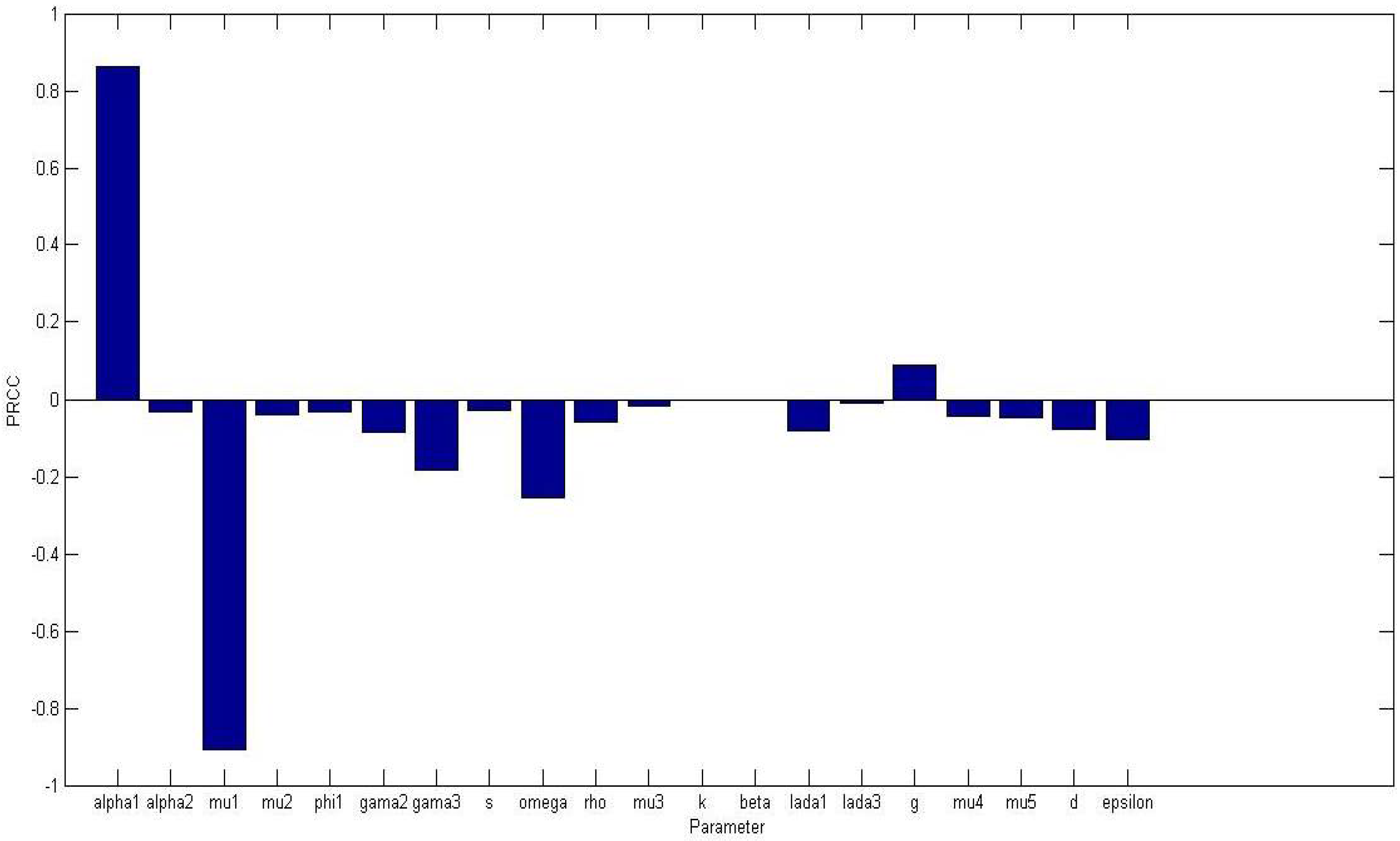
4. Uncertainty and Sensitivity Analysis

In this section, we explore the dependence of the model solutions on the parameter values. We are able to figure-out a feasible range of parameter values and determine the most critical parameters in the model. We employed a similar method, which is discussed in detail by [20,33], using Latin Hypercube Sampling (LHS) for studying the uncertainty analysis and the Partial Rank Correlation Coefficient (PRCC) for analyzing the sensitivity analysis indexes of the parameters. LHS/PRCC was ran and analyzed with a sample size of 100. The choice of this sample size is due to the fact that PRCC produces accurate results for a lower sample size compared to other technique, such as eFAST [33].

Uncertainty and sensitivity analysis were performed on all non-dimensional system parameters in the system (5) with the aim of determining the most sensitive parameters to the model. The parameter baseline values in

Table 1. Description of parameters in the model.

Parameter	Symbol	Value	Unit	Refs
Per capita growth rate of normal cells	${\alpha }_1$	0.70	day−1	[12]
Per capita growth rate of tumor cells	${\alpha }_2$	0.514	day−1	[5]
Natural death rate of normal cells	${\mu }_1$	0.00003	day−1	Assumed
Natural death rate of tumor cells	${\mu }_2$	0.01	day−1	[7]
Rate of inhibition of normal cells	${\varphi }_1$	6 × 10−8	day−1	[1]
Tumor cells death rate due to immune response	${\gamma }_2$	3 × 10−6	day−1	[12]
Interaction coefficient rate with immune response	${\gamma }_3$	1 × 10−7	day−1	[5]
Source rate of immune cells	$s$	1.3 × 104	day−1	[12]
Source rate of estrogen	$ϵ$	1.3 × 104	day−1	est
Immune threshold rate	$\omega$	3 × 105	day−1	[5]
Immune response rate	$\rho$	0.20	day−1	[13]
Natural death rate of immune cells	${\mu }_3$	0.29	day−1	[5]
Efficacy of anti-cancer drug	$k$	0–1	day−1	Assumed
Supplement for immune booster	$\beta$	0.01	day−1	est
Tumor formation rate as a result of DNA damage by excess estrogen	${\lambda }_1$	0.20	(Pg/mL)−1day−1	est
Immune suppression rate due to excess estrogen	${\lambda }_3$	0.002	day−1	est
Assume constant of value of decay factor	$g$	0.1	day−1	est
Natural death rate of estrogen	${\mu }_4$	0.97	day−1	[19]
Death rate due to ketogenic diet	${\mu }_5$	2.0	day−1	est
Constant rate of ketogenic diet	$d$	0.5	day−1	est

were varied in the range of 25%. Figure 1 displays a bar graph of PRCCs plotted against the homogeneous parameter value with tumor compartment as the baseline dependent variable. The parameters that are significantly positively correlated with tumor cells, at $P<0.05$ level of significance, are ${\alpha }_1,g$ while ${\mu }_1,{\gamma }_3$, and $\omega$ are significantly negatively correlated. An increase in the production of normal cells ${\alpha }_1$, leads to higher numbers of normal cells, thus the higher the ${\alpha }_1$, the higher the normal cells. 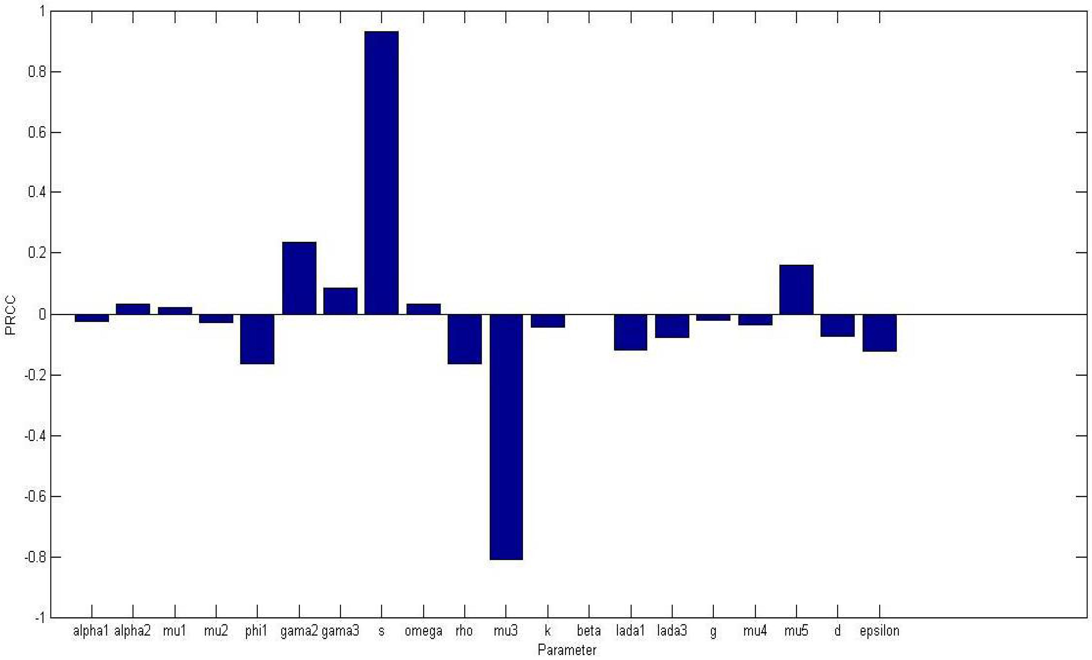While Figure 2 displays a bar graph of PRCCs plotted against the homogeneous parameter value with tumor compartment as the baseline dependent variable. The most sensitive parameters are shown to be $P-values$ of $s,{\gamma }_2,{\mu }_3$ and $\rho$ are less than 0.01.

5. Analysis of Optimal Control

In this section, we formulated a corresponding optimal control problem for the model in the system (5) considering ketogenic-diet and anti-cancer drugs as control interventions to minimize the breast cancer and tumor burden at final time. The units of cells were normalized in order for the carrying capacity of normal cells to be kept above threshold of $0\le t\le t_f$ [34,35,36]. On the other hand, the aim is to reduce the tumor-size which indicates the degree of the disease in the body and it requires the application of as much anti-cancer drugs as much as possible. However, it also minimized the systemic cost, which is based on the quantities of anti-cancer drugs, since large drug concentrations can be harmful and cause toxic side effects. In brief, the drug doses were minimized because the smaller the dose, the better. Then, we formulated the objective functional $J_1$

$$J_1(u_1,u_2)={\displaystyle {\int }_0^{T_f}}\left(A_{1}T(t)+A_{2}E(t)+\frac{1}{2}{A}_3{u}_1^2(t)+\frac{1}{2}{A}_4{u}_2^2(t)\right)dt$$

(8)

System equations (5) is subject to:

$$\begin{array}{ll}\hfill & \frac{dN}{dt}=N{\alpha }_1-{\mu }_1{N}^2-{\varphi }_{1}TN-\left(1-u_1(t)\right)\left({\lambda }_{1}NE\right)\hfill \\ \hfill & \frac{dT}{dt}=\left(1-u_2(t)\right)T{\alpha }_2-{\mu }_2{T}^2-{\gamma }_{2}MT-{\mu }_{5}T+\left(1-u_1(t)\right)\left({\lambda }_{1}NE\right)\hfill \\ \hfill & \frac{dM}{dt}=s\beta +\frac{\rho MT}{\omega +T}-{\gamma }_{3}MT-{\mu }_{3}M-\left(\left(1-u_1(t)\right)\frac{{\lambda }_{3}ME}{g+E}\right)\hfill \\ \hfill & \frac{dE}{dt}=\left(1-u_1(t)\right)ϵ-{\mu }_{4}E\hfill \end{array}$$

(9)

$J_1$ involves a quadratic control. In [37,38,39,40,41], it was established that quadratic control in the treatment terms has the added benefit of keeping the tumor in check both when it is small or large in size. The authors further explained that the quadratic control allows for a weaker treatment to minimize the toxic side-effects while permitting the system to maintain a low tumor size.

Furthermore, for us to address the tumor-to-therapy trade-off, we established the existence of an optimal control; by following the approach in [37,41,42], which required an analysis of the super-solutions (that is, the upper bounds on solutions) of the system (5). As soon as we were able to show that the system is bounded, we established the existence of an optimal control using a result from [43]. In addition, we proved that there exists an optimal control that minimizes the objective functional; using the established approach of [37,38,39,40,44]. We use the fact that super-solutions $\overline{N}$, $\overline{T}$, $\overline{M}$, $\overline{E}$ of

$$\begin{array}{l}\frac{d\overline{N}}{dt}=N{\alpha }_1,\frac{d\overline{T}}{dt}=T{\alpha }_2(1-u_2),\hfill \\ \frac{d\overline{M}}{dt}=s\beta +\frac{\rho MT}{\omega +T},\frac{d\overline{E}}{dt}=1\hfill \end{array}$$

(10)

are bounded on a finite time interval. Since the sub-solutions are zero, the result obtained shows that our system is bounded. Since we have a bounded system, our next task was to establish the existence of the optimal control using a result from [43].

Existence of an Optimal Control

Theorem 6.

Given the objective functional in (8), where$U=\{u_i^{*}(t),Lebesguemeasure:0\le u_i^{*}(t)\le 1,\forall t\in [0,t]\}$subject to system (9) with$N(0)=N_0$, $T(0)=T_0$, $M(0)=M_0$, and$E(0)=E_0$, then there exists an optimal control$\overline{u_i^{*}}$such that${{\displaystyle min}}_{\overline{u_i^{*}}(t)\in [0,1]}{J}_1\overline{(u_i^{*}})=J_1(u_i^{*}(t))$if the following conditions holds:

• $f$ is not empty;
• The admissible control set $U$ is closed and convex;
• Each right hand side of the state system is continuous, is bounded above by the sum of the bounded control and the state, and can be written as a linear function of $\overline{u_i^{*}(t)}$ with coefficients depending on time and the state;
• The integrand of $J_1\overline{(u_i^{*}})$ is convex on $U$ and is bounded below by $-c_2+c_1{\overline{u}}^2$ with $c_1>0$.

Proof. 

Since the system (9) has bounded coefficients and the solutions are bounded on the finite time interval, we can apply the result of [45], to obtain the existence of the solution of the system (9). Furthermore, we note that $U$ is closed and convex by definition. For the third conditions, the right hand side of the system (9) must be continuous. The right hand side is continuous since the denominators of all fractions from the right hand side of the system consists solely of positive entities. We let $\overleftarrow{\varphi }(t,\overleftarrow{X})$ be right hand side of the system (9) except for the terms of $\overline{u_i^{*}}$ and define.

$$|\overleftarrow{f}(t,\overleftarrow{X},u_i^{*})|=\overleftarrow{\varphi }(t,\overleftarrow{X})+\left(\begin{array}{c}0\\ {\lambda }_{1}NE\\ 0\\ u_1\\ \end{array}\right),with\overleftarrow{X}=\left(\begin{array}{c}N\\ T\\ M\\ E\\ \end{array}\right)$$

using the boundedness of the solutions (10), we have

$$|\overleftarrow{f}(t,\overleftarrow{X},u_i^{*})|\le \left|\begin{array}{c}\left(\begin{array}{cccc}{\alpha }_1& 0& 0& 0\\ 0& {\alpha }_2(1-u_2)& 0& 0\\ 0& 0& \rho & 0\\ 0& 0& 0& 0\\ & & & \end{array}\right)\left(\begin{array}{c}N\\ T\\ M\\ E\\ \end{array}\right)\end{array}\right|+\left|\begin{array}{c}\left(\begin{array}{c}0\\ (1-u_1){\lambda }_{1}NE\\ s\beta \\ -u_1ϵ\\ \end{array}\right)\end{array}\right|\le c_1\left(|\overleftarrow{X}|+|\overleftarrow{u_i^{*}}|\right)$$

where $c_1$ depends on the coefficients of the system. For the fourth condition, we need to show

$$J\left(t,T,E,(1-P_i)u_i+P_i{V}_i\right)\le (1-P_i)J\left(t,T,E,u_i\right)+P_i(t,T,E,V_i)$$

we analyze the difference of

$$J\left(t,T,E,(1-P_i)u_i+P_i{V}_i\right)-\left[(1-P_i)J\left(t,T,E,u_i\right)+P_i(t,T,E,V_i)\right]$$

$$\begin{array}{l}=T(t)+E(t)+\frac{ϵ}{2}\left(u_i^2-2P_i{u}_i^2+P_i^2{u}_i^2+P_i^2{V}_i^2-2P_i^2{V}_i^2{u}_i^2+2P_i{V}_i{u}_i\right)\hfill \\ -\left(T(t)+E(t)+\frac{ϵ}{2}{u}_i^2-\frac{ϵ}{2}{P}_i{u}_i^2+\frac{ϵ}{2}{P}_i{V}_i^2\right)\hfill \end{array}$$

$$=\frac{ϵ}{2}(P_i^2-P_i)(u_i-V_i{)}^2$$

since, $P_i\in (0,1)$ implies $(P_i^2-P_i)<0$ and ${(u_i-V_i)}^2>0$ but $(P_i^2-P_i)<0$, which implies $\frac{ϵ}{2}(P_i^2-P_i)(u_i-V_i{)}^2$ is negative. This implies that,

$$J\left(t,T,E,(1-P_i)u_i+P_i{V}_i\right)\le (1-P_i)J\left(t,T,E,u_i\right)+P_i(t,T,E,V_i)$$

Lastly,

$$T(t)+E(t)+\frac{ϵ}{2}{u}_i^2(t)\ge \frac{ϵ}{2}{u}_i^2(t)\ge -c+\frac{ϵ}{2}{u}_i^2(t)$$

which gives $-c+\frac{ϵ}{2}{u}_i^2(t)$ as the lower bound. With the existence of the optimal control established, we now characterized the optimal control using the Pontryagin’s maximum principle [11]. The constants $A_1,A_2,A_3$ and $A_4$ are a measure of the relative cost of the interventions over $\left[0,T\right]$. The optimal control problem is that of finding optimal functions $(u_1^{*}(t),u_2^{*}(t))$ such that

$$J_1(u_1^{*}(t),u_2^{*}(t))=\underset{\mathsf{\Omega }}{{\displaystyle \min }}{J}_1(u_1(t),u_2(t))$$

(11)

where

$$\mathsf{\Omega }=\left\{u_1(t)\&u_2(t):0\le u_1(t)\le u_{1max}\mathrm{,0}\le u_2(t)\le u_{2max},t\in [0,T_f]\right\}$$

□

Three different control strategies are explored. This approach can be used to test various options. However, we only looked at the following three alternatives:

• Strategy 1: Anti-cancer drug treatment control on tumor cells (control $u_1(t)$ only);
• Strategy 2: Ketogenic diet control on excess estrogen and tumor cells (control $u_2(t)$ only);
• Strategy 3: Anti-cancer drug and ketogenic diet treatment combined control on tumor cells growth and excess estrogen (controls $u_1(t)$ and $u_2(t)$).

Thus, strategies (1–3) use the objective functional (8). We assumed that there are practical limitations on the maximum rate at which the anti-cancer treatment may be applied in a given time period. We defined the positive constant $u_{max}$ accordingly. We also define the set $\mathsf{\Omega }$ of admissible controls to be all Lebesgue measurable functions that take on values in the control set [13,46,47] $u=\left[0,u_{max}\right]$ almost everywhere on $\left[0,T\right]$. We sought an optimal control $u^{*}\in \mathsf{\Omega }$ in (11) [13]. In order to find the optimal solutions, we first traced the Lagrangian and Hamiltonian for the optimal control problem (8) and (9). The Lagrangian of the optimal control problem is given by:

$$L(N,T,M,E,u_1,u_2)=A_{1}T(t)+A_{2}E(t)+\frac{1}{2}{A}_3{u}_1^2(t)+\frac{1}{2}{A}_4{u}_2^2(t)$$

(12)

For the purpose of the necessary conditions for optimal control functions with the help of Pontryagin’s maximum principle [11]. We define the Hamiltonian, $H$ for the control problem of the system (8) and (9)

$$H=L(N,T,M,E,u_1,u_2)+{\theta }_1{N}^{\prime }+{\theta }_2{T}^{\prime }+{\theta }_3{M}^{\prime }+{\theta }_4{E}^{\prime }$$

(13)

where L is the Lagrangian function (12),

$$H=(\begin{array}{c}{A}_{1}T(t)+A_{2}E(t)+\frac{1}{2}{A}_3{u}_1^2(t)+\frac{1}{2}{A}_4{u}_2^2(t)\\ +{\theta }_1\left(N{\alpha }_1-{\mu }_1{N}^2-{\varphi }_{1}TN-\left(1-u_1(t)\right)\left({\lambda }_{1}NE\right)\right)\\ +{\theta }_2\left(\left(1-u_2(t)\right)T{\alpha }_2-{\mu }_2{T}^2-{\gamma }_{2}MT-{\mu }_{5}T+\left(1-u_1(t)\right)\left({\lambda }_{1}NE\right)\right)\\ +{\theta }_3\left(s\beta +\frac{\rho MT}{\omega +T}-{\gamma }_{3}MT-{\mu }_{3}M-\left(\left(1-u_1(t)\right)\frac{{\lambda }_{3}ME}{g+E}\right)\right)\\ +{\theta }_4\left(\left(1-u_1(t)\right)ϵ-{\mu }_{4}E\right)\\ \end{array}$$

where ${\theta }_1,{\theta }_2,{\theta }_3,{\theta }_4$ are the adjoints variables for the states N, T, M, E. However, with the help of Pontryagin’s Maximum Principle, we obtained a minimized Hamiltonian that minimizes the objective function or cost functional. We applied Pontryagin’s Maximum Principle [11], to characterize the optimal control pair $u_1^{*}\&u_2^{*}$ in the following result.

Theorem 7.

Given optimal control variables$u_1^{*}\&u_2^{*}$and$N^{*},T^{*},M^{*}\&E^{*}$are corresponding optimal state variables of the control system (8) and (9). Then there exists the adjoint variable${\theta }_i=\left({\theta }_1,{\theta }_2,{\theta }_3,{\theta }_4\right)\in {\Re }_{+}^4$that satisfies the following equations.

$$\begin{array}{ll}\hfill & \frac{d{\theta }_1}{dt}=2{\theta }_1{\mu }_{1}N+{\varphi }_1{\theta }_{1}T+({\theta }_1+{\theta }_2)\left(1-u_2(t)\right){\lambda }_{1}E-{\alpha }_1{\theta }_1\hfill \\ \hfill & \frac{d{\theta }_2}{dt}=-A_1+{\theta }_1{\varphi }_{1}N+{\theta }_2\left(2T{\mu }_2+{\gamma }_{2}M+{\mu }_5-{\alpha }_2(1-u_2)\right)+{\theta }_3\left({\gamma }_{3}M-\frac{\rho \omega M}{{(\omega +T)}^2}\right)\hfill \\ \hfill & \frac{d{\theta }_3}{dt}={\theta }_2{\gamma }_{2}T-\rho {\theta }_{3}T+{\gamma }_3{\theta }_{3}T+{\mu }_3{\theta }_3+{\theta }_3\left((1-u_1)\frac{{\lambda }_{1}E}{g+E}\right)\hfill \\ \hfill & \frac{d{\theta }_4}{dt}=-A_2+({\theta }_1-{\theta }_2)(1-u_1){\lambda }_{1}N-{\theta }_3\left((1-u_1)\frac{{\lambda }_{3}Mg}{{(g+E)}^2}\right)-{\theta }_4{\mu }_4\hfill \end{array}$$

(14)

with transversality conditions

$${\theta }_1(T_f)={\theta }_2(T_f)={\theta }_3(T_f)={\theta }_4(T_f)=0$$

The corresponding optimal controls $u_1^{*}\&u_2^{*}$ are given as,

$$u_1^{*}=min\left\{max\left\{0,\frac{1}{A_3}\left({\theta }_2{\lambda }_1{N}^{*}{E}^{*}+{\theta }_3ϵ-{\theta }_1{\lambda }_1{N}^{*}{E}^{*}-\frac{{\theta }_3{\lambda }_3{M}^{*}{E}^{*}}{g+E^{*}}\right)\right\}\mathrm{,1}\right\}$$

(15)

and

$$u_2^{*}=min\left\{max\left\{0,\frac{1}{A_4}\left({\theta }_2{\alpha }_2{T}^{*}\right)\right\}\mathrm{,1}\right\}$$

(16)

Proof. 

Let $u_1^{*}\&u_2^{*}$ be the given optimal control functions and $N^{*},T^{*},M^{*}\&E^{*}$ be the corresponding optimal state variables of the system (9) that minimize the cost functional or objective (8). Then by Pontryagin’s maximum principle [11], there exists adjoint variables (14) ${\theta }_1,{\theta }_2,{\theta }_3\&{\theta }_4$ which satisfy the following equations

$$\begin{array}{l}\frac{d{\theta }_1}{dt}=-\frac{\partial H}{\partial N},\frac{d{\theta }_2}{dt}=-\frac{\partial H}{\partial T},\frac{d{\theta }_3}{dt}=-\frac{\partial H}{\partial M},\frac{d{\theta }_4}{dt}=-\frac{\partial H}{\partial E}\hfill \end{array}$$

with transversality conditions

$${\theta }_1(T_f)={\theta }_2(T_f)={\theta }_3(T_f)={\theta }_4(T_f)=0$$

where H is the Hamiltonian and defined as

$$H(N,T,M,E,u_1,u_2,\theta )=L(N,T,M,E,u_1,u_2)+{\theta }_1{N}^{\prime }+{\theta }_2{T}^{\prime }+{\theta }_3{M}^{\prime }+{\theta }_4{E}^{\prime }$$

$$H=(\begin{array}{c}{A}_{1}T(t)+A_{2}E(t)+\frac{1}{2}{A}_3{u}_1^2(t)+\frac{1}{2}{A}_4{u}_2^2(t)\\ +{\theta }_1\left(N{\alpha }_1-{\mu }_1{N}^2-{\varphi }_{1}TN-\left(1-u_1(t)\right)\left({\lambda }_{1}NE\right)\right)\\ +{\theta }_2\left(\left(1-u_2(t)\right)T{\alpha }_2-{\mu }_2{T}^2-{\gamma }_{2}MT-{\mu }_{5}T+\left(1-u_1(t)\right)\left({\lambda }_{1}NE\right)\right)\\ +{\theta }_3\left(s\beta +\frac{\rho MT}{\omega +T}-{\gamma }_{3}MT-{\mu }_{3}M-\left(\left(1-u_1(t)\right)\frac{{\lambda }_{3}ME}{g+E}\right)\right)\\ +{\theta }_4\left(\left(1-u_1(t)\right)ϵ-{\mu }_{4}E\right)\\ \end{array}$$

from the optimality condition, we have

$$\begin{array}{l}\frac{\partial H}{\partial u_1}=0,at{u}_1=u_1^{*}and\frac{\partial H}{\partial u_2}=0,at{u}_2=u_2^{*}\hfill \end{array}$$

which implies that

$$0=\frac{\partial H}{\partial u_1}=A_3{u}_1+{\theta }_1{\lambda }_{1}NE-{\theta }_2{\lambda }_{1}NE+{\theta }_3\frac{{\lambda }_{3}ME}{g+E}-{\theta }_4ϵ$$

$$0=\frac{\partial H}{\partial u_1}=A_4{u}_2-{\theta }_2{\alpha }_{2}T$$

Hence, we obtain (see [10])

$$u_1^{*}=\frac{1}{A_3}\left\{{\theta }_1{\lambda }_{1}NE+{\theta }_4ϵ-{\theta }_1{\lambda }_{1}NE-{\theta }_3\frac{{\lambda }_{3}ME}{g+E}\right\}$$

(17)

$$u_2^{*}=\frac{1}{A_4}\left\{{\theta }_2{\alpha }_{2}T\right\}$$

(18)

Thus we have (17) and (18).

By standard control arguments involving the bounds on the controls, we conclude that (15) and (16) can be written in this form

$$u_1^{*}=(\begin{array}{cc}0& if\frac{1}{A_3}\left({\theta }_1{\lambda }_{1}NE+{\theta }_4ϵ-{\theta }_1{\lambda }_{1}NE-{\theta }_3\frac{{\lambda }_{3}ME}{g+E}\right)<0\\ \frac{1}{A_3}\left({\theta }_1{\lambda }_{1}NE+{\theta }_4ϵ-{\theta }_1{\lambda }_{1}NE-{\theta }_3\frac{{\lambda }_{3}ME}{g+E}\right)& if0\le \frac{1}{A_3}\left({\theta }_1{\lambda }_{1}NE+{\theta }_4ϵ-{\theta }_1{\lambda }_{1}NE-{\theta }_3\frac{{\lambda }_{3}ME}{g+E}\right)\le 1\\ 1& if\frac{1}{A_3}\left({\theta }_1{\lambda }_{1}NE+{\theta }_4ϵ-{\theta }_1{\lambda }_{1}NE-{\theta }_3\frac{{\lambda }_{3}ME}{g+E}\right)>1\end{array}$$

and

$$u_2^{*}=(\begin{array}{cc}0& if\frac{1}{A_4}\left({\theta }_2{\alpha }_2{T}^{*}\right)<0\\ \frac{1}{A_4}\left({\theta }_2{\alpha }_2{T}^{*}\right)& if0\le \frac{1}{A_4}\left({\theta }_2{\alpha }_2{T}^{*}\right)\le 1\\ 1& if\frac{1}{A_4}\left({\theta }_2{\alpha }_2{T}^{*}\right)>1\end{array}$$

□

However, we discuss the numerical solution of the optimality system and the corresponding results of varying the optimal controls $u_1\&u_2$ the parameter choices, and the interpretations from various cases.

6. Numerical Simulations and Discussion

A picture of the dynamical behavior of breast cancer cells in the presence of normal cells, tumor cells, immune cells, and estrogen is given by the numerical simulations of the model (5). The optimal control is acquired by solving the optimality system of four ordinary differential equations from the state variables and the adjoint system. An iterative scheme is used to solve the optimality system. All the numerical simulations were executed in MAPLE 18. We employed the forward-backward scheme method, beginning with an initial guess for optimal controls and solved the optimal state system forward in time and after that solved the adjoint state system backward in forward using the finite difference scheme in MAPLE. The two controls were then updated by using a convex combination of the previous controls as well as the characterization (17) and (18). The entire process was repeated until the values of the unknown at the previous iterations were closed to the one at the current iteration [39,41]. Key parameters are also noted in stabilizing the model in system (5), for example: ketogenic diet, anti-cancer, and immune booster. The initial values of variables are N(0) = 2000, T(0) = 800, M(0) = 500, E(0) = 20 and $s=1.3\times {10}^4$ adopted from [12]. All parameter values used for the numerical simulation are stated in Table 1 above.

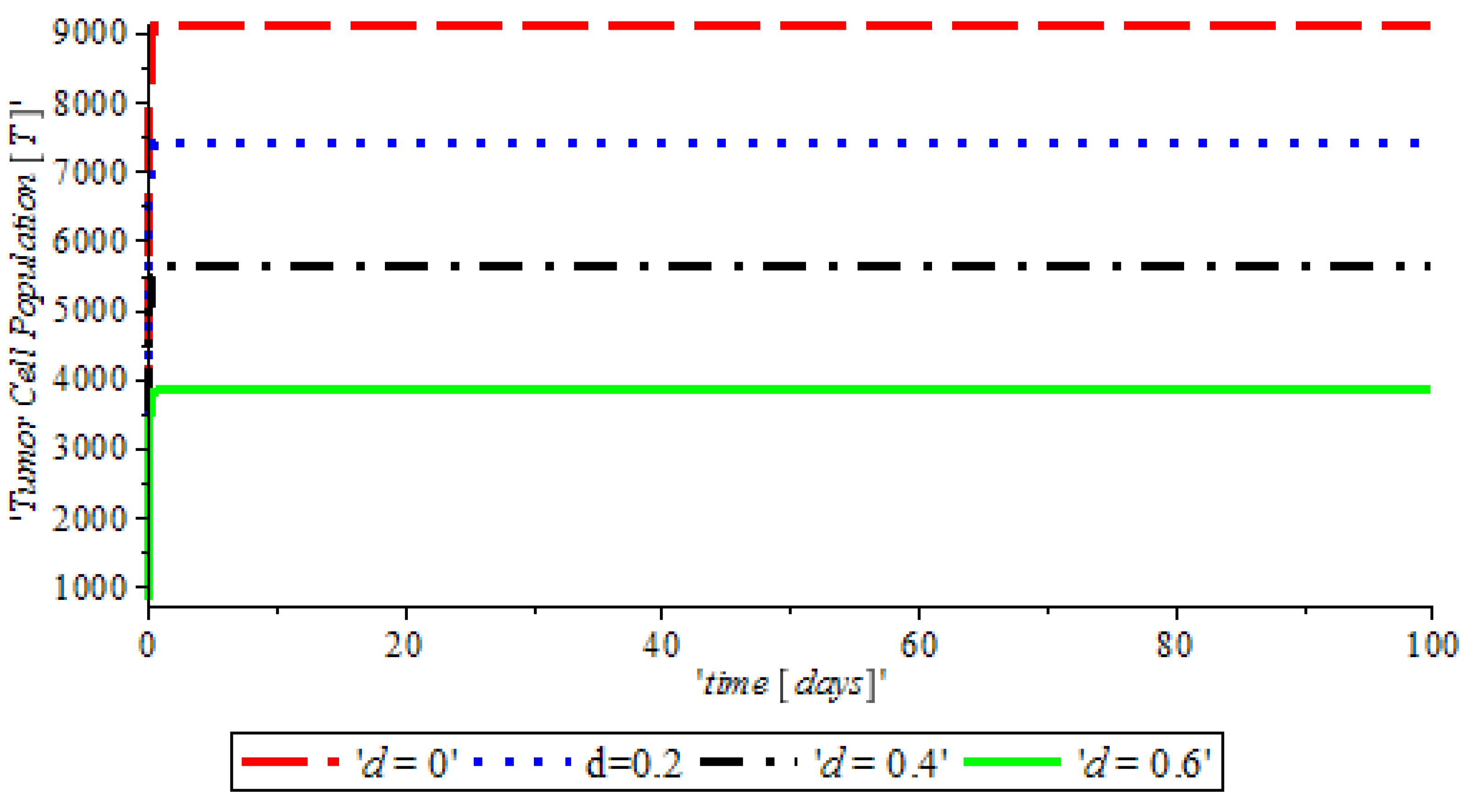
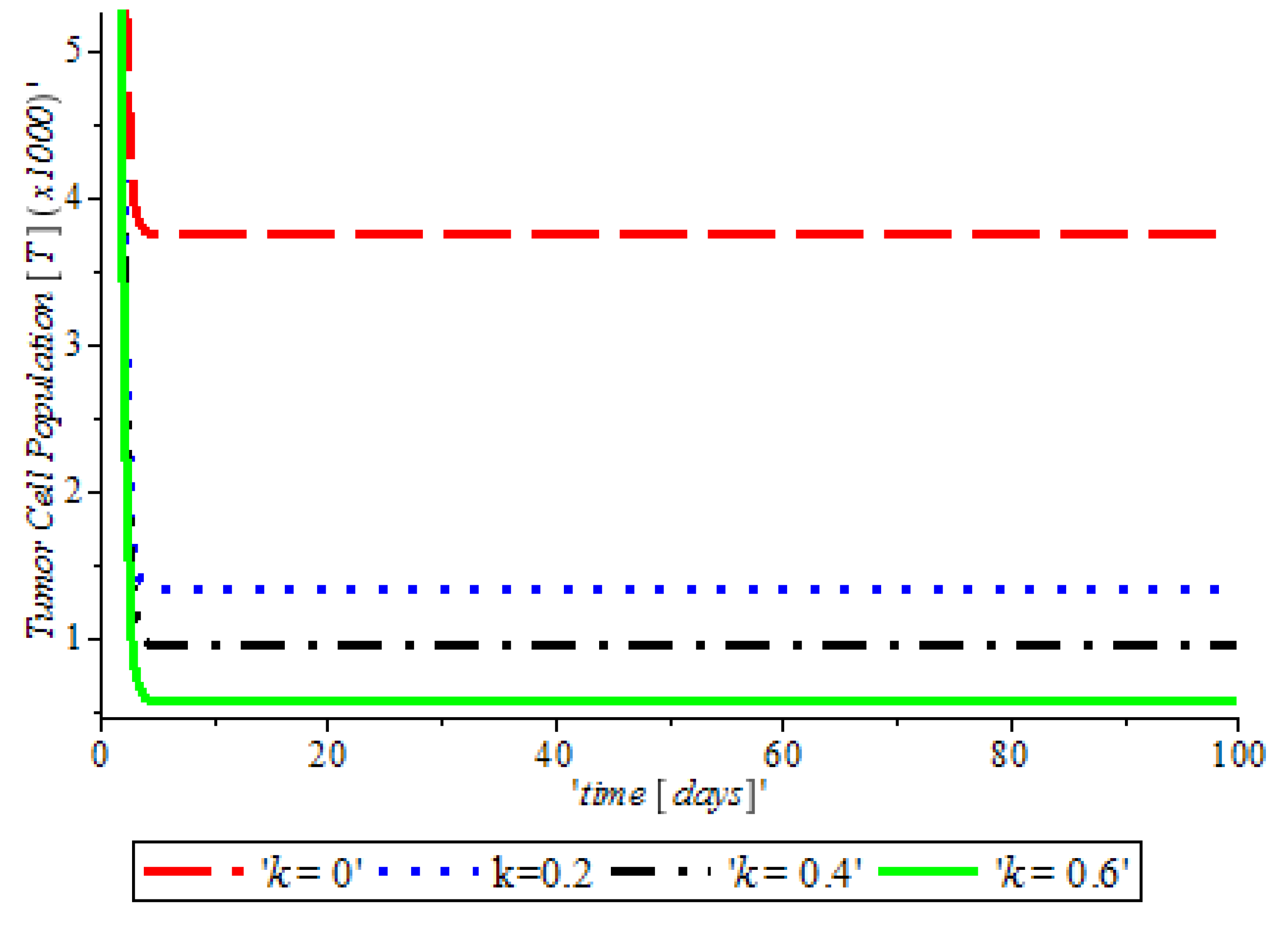
Figure 3, indicates that the introduction of a ketogenic diet results in a reduction of activities of cancer cells and we also note that too much of a ketogenic diet will result in ketoacidosis. Ketoacidosis is the combination of ketosis and acidosis. Ketosis is the accumulation of substances called ketone bodies and acidosis is the increased acidity of the blood which can cause frequent urination (Polyuria), poor appetite, and a loss of consciousness. Therefore, our ketogenic diet’s parameter rate is best at $d=0.6$ and it can complement the activity of the anti-cancer drug (Tamoxifen). 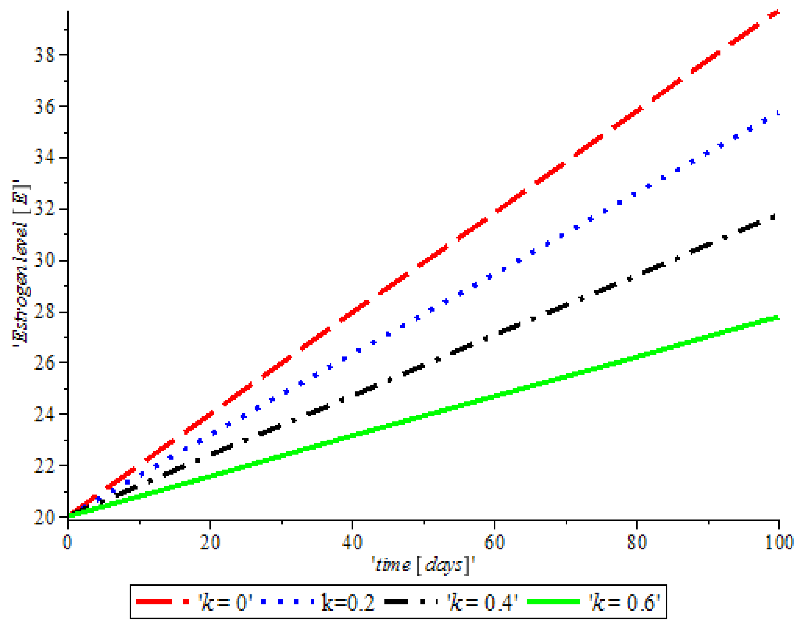Figure 4, shows the impact of anti-cancer drugs in reducing the production of excess estrogen in the system, but when there is less production of estrogen there will not be a rapid activation of the growth factor that expresses breast normal cells. However, the rapid production of estrogen results in abnormal breast cells expression, which will lead to breast cancer. Figure 5 shows the obvious effectiveness of anti-cancer drugs on tumor cells when there is no supply of nutrient or glucose to cancer cells.

Furthermore, Figure 6 illustrates that the red line $\beta =0$ shows that during cancer formation the activities of both innate and adaptive reduces drastically, which is due to the expression of other proteins apart from those proteins that are responsible for the activation of the immune response, such as an immune booster introduced to the system, which reactivates the activities of the immune response towards the cancer cells.

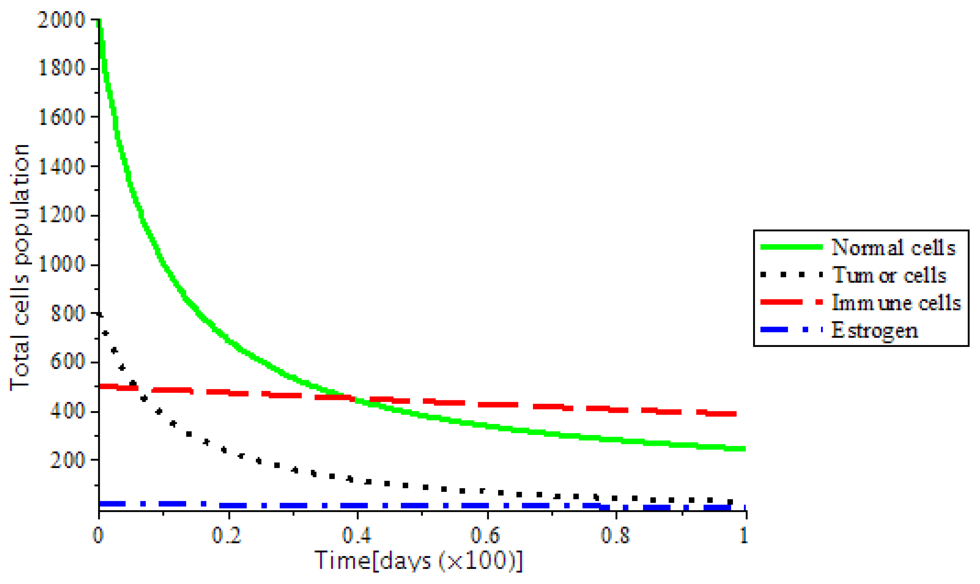
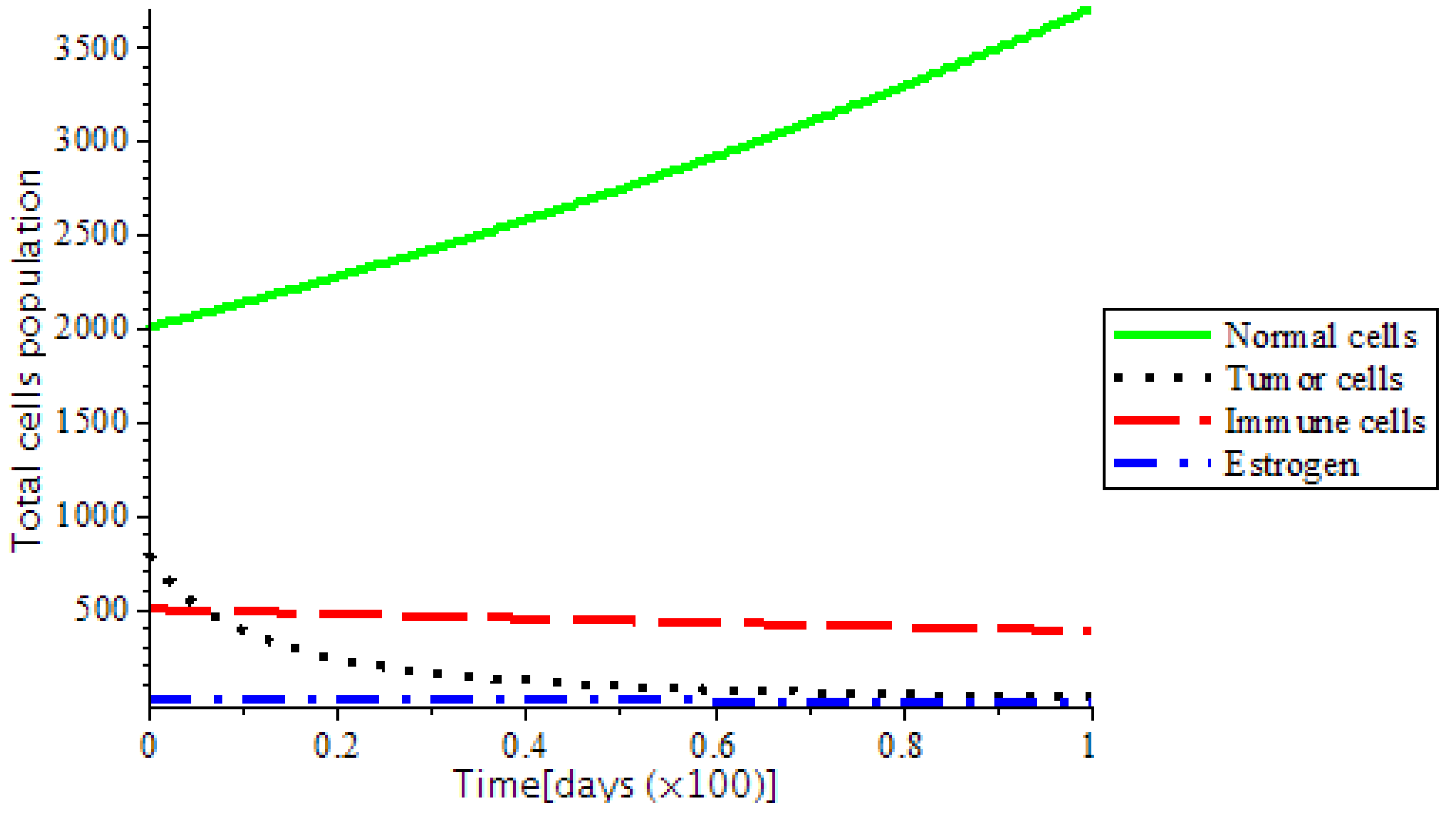
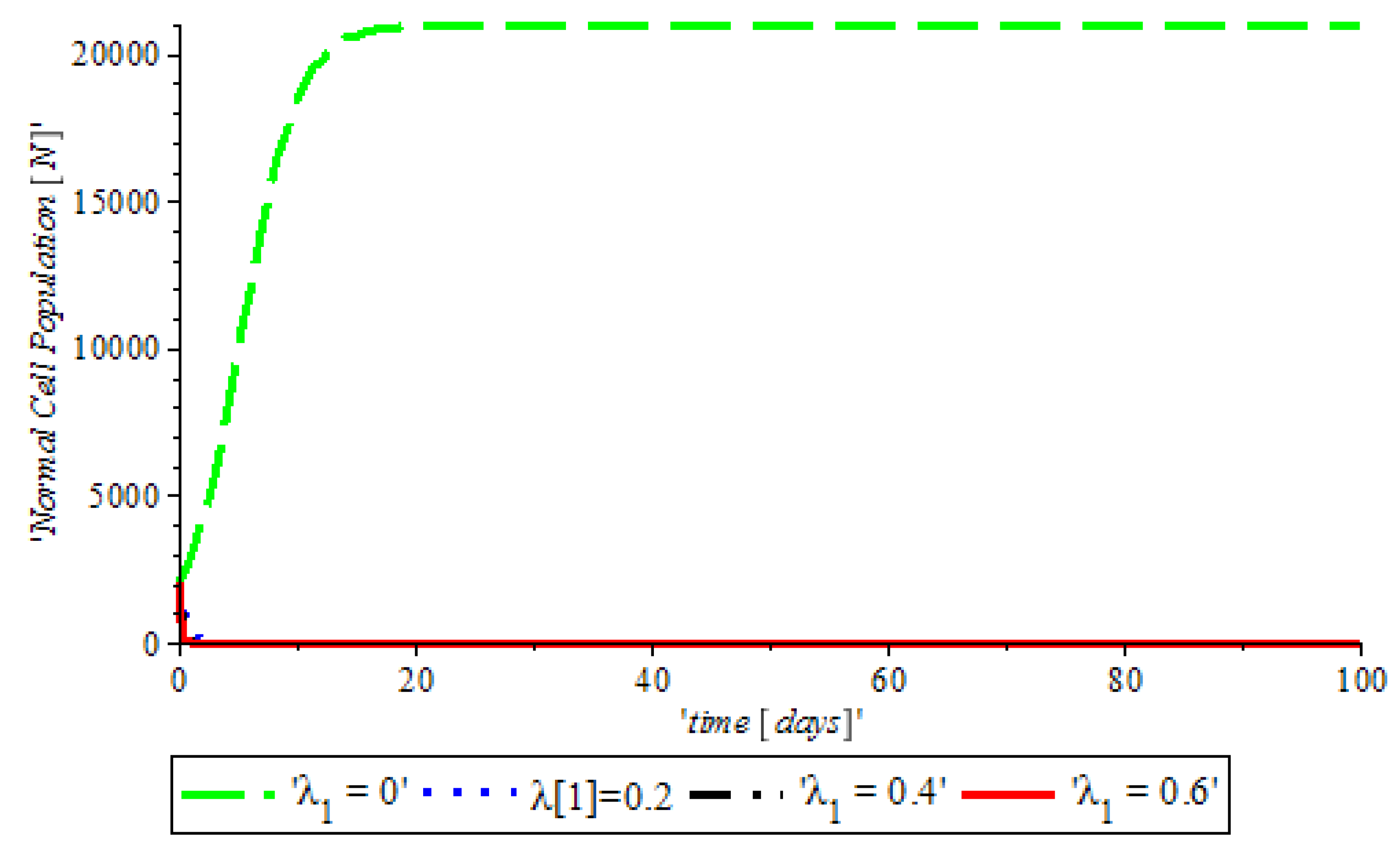
The presence of abnormal estrogen level without anti-cancer drugs or a ketogenic diet will lead the system into critical condition and became unstable as shown in Figure 7. However, the system became stable as we introduced treatments, such as chemotherapy and the ketogenic diet as represented in Figure 8. In addition, Figure 9, indicates that there is DNA damage at ${\lambda }_1=0$, which occurs naturally as a result of metabolic or hydrolytic processes. It is as a result of the Tumor Suppressor Gene (TSG), which is able to control the activity of DNA gene repair successfully. On the other hand, at ${\lambda }_1=0.2,0.4,0.6$ showed that TSG (such as BRCA 1, BRCA 2, P53) compromised the pathway that leads cells to grow uncontrollably and later form a tumor or it leads to accelerated aging.

However, the mathematical analysis of the model produced six equilibrium points. All the points have epidemiological implications in relation to explaining the dynamics of breast cancer growth. $P_0$ represents the situation where there is tumor-free equilibrium, that is when only tumor cell population has died off due to competition with other cells. $P_{d1}$ represents Type 1 dead equilibrium point where both normal cells and tumor cells die-off as a result of breast tissue removal through mastectomy surgery or death. This is because overtime the cancer cells which are depending on estrogen to develop into independent cells that grow regardless of estrogen receptors. $P_{d2}$ could be described by Type 2 dead equilibrium point where normal cells were only forced to extinction leaving the tumor cells surviving. $P_{d3}$ represent Type 3 dead equilibrium point which means immune system is weak and it cannot fight the tumor cells which eventually overpower normal cells and forced it to extinction. $P_{d4}$ show that Type 4 dead equilibrium point where ketogenic diet is not effective, immune booster is not active which lead to tumor cell over-compete normal cells as a result of infusion of excess estrogen to the body system.

We categorised this as ”dead” because biologically there is no recovery of damaged normal cells since they have died off of the cell population. It could be as a result of anti-cancer drug that destroy red blood cells which affected normal cells.

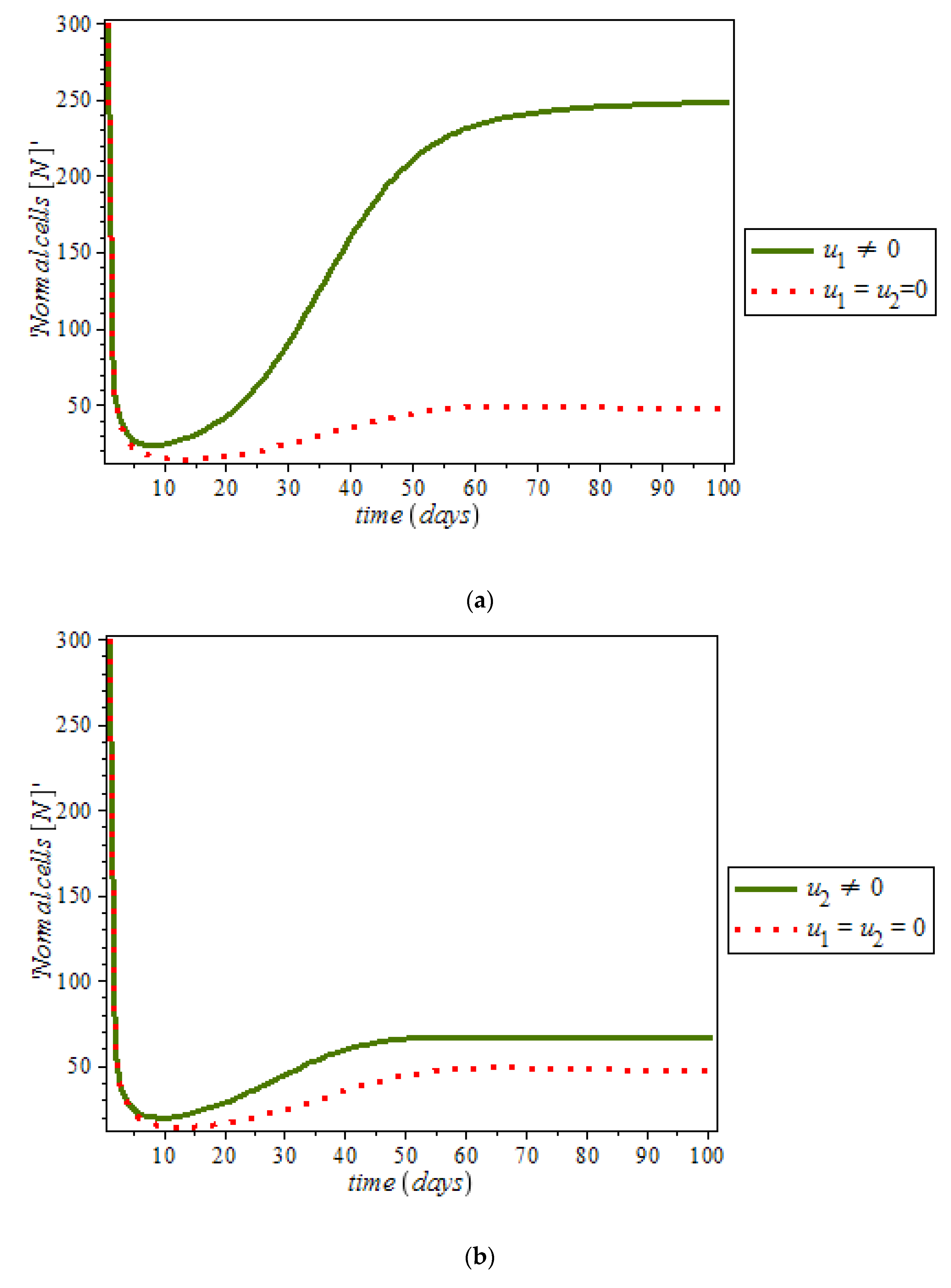
Effects of Control on the System (9)

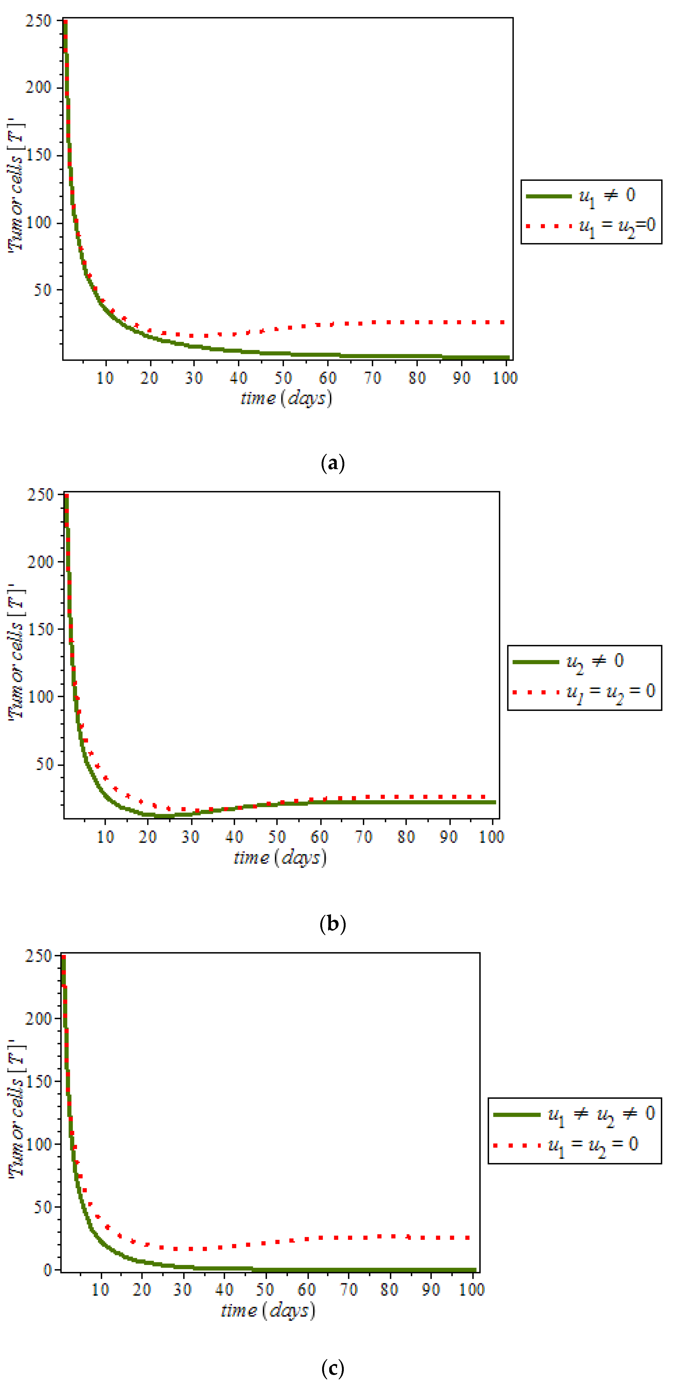
By numerical simulation, optimal single control of anti-cancer drugs measure $u_1$ and ketogenic-diet optimal control measure $u_2$ are shown in Figure 10a,b respectively; where (red dots line) represented tumor cells and (solid green line) represented normal cells. Figure 10c is the use of combination of two control therapies which have significant impact on the increase of normal cells population against time. However, all the strategies are effectively restrain the tumor growth, they cannot totally eliminate a large tumor in 100 days. In Figure 11, optimal control using anti-cancer drugs and ketogenic diet as we optimized the system (54) with the objective function $J$ for breast cancer model. It was observed that the combination of the two controls resulted in appreciable decreases in the number of tumor cells population in the presence of control (solid green line) while (dots red line) in the case of uncontrolled. However, tumor growth is driven to a very low but non-zero level.

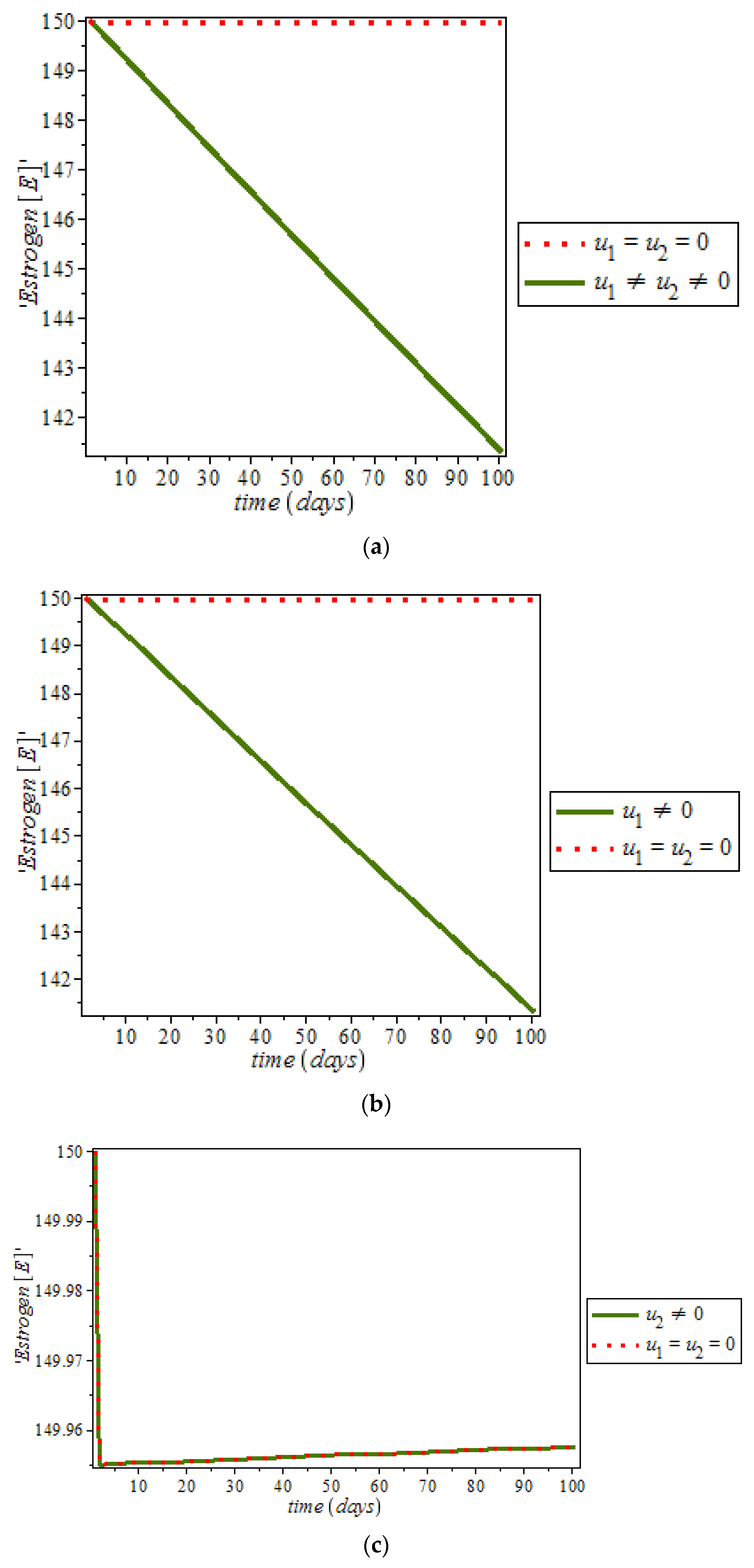
Furthermore, it was noticed from Figure 12, that the level of estrogen was reduced drastically in the presence of controls (solid green line) against the constant increase level of estrogen (dots red line) in uncontrolled cases. However, anti-cancer drugs (for example Tamoxifen) blocks estrogen receptors on breast cells, that is, it stops estrogen from connecting to the cancer cells while tamoxifen also acts like an anti-estrogen in breast cells; it acts like an estrogen in other tissues like the uterus and the bones [48]. 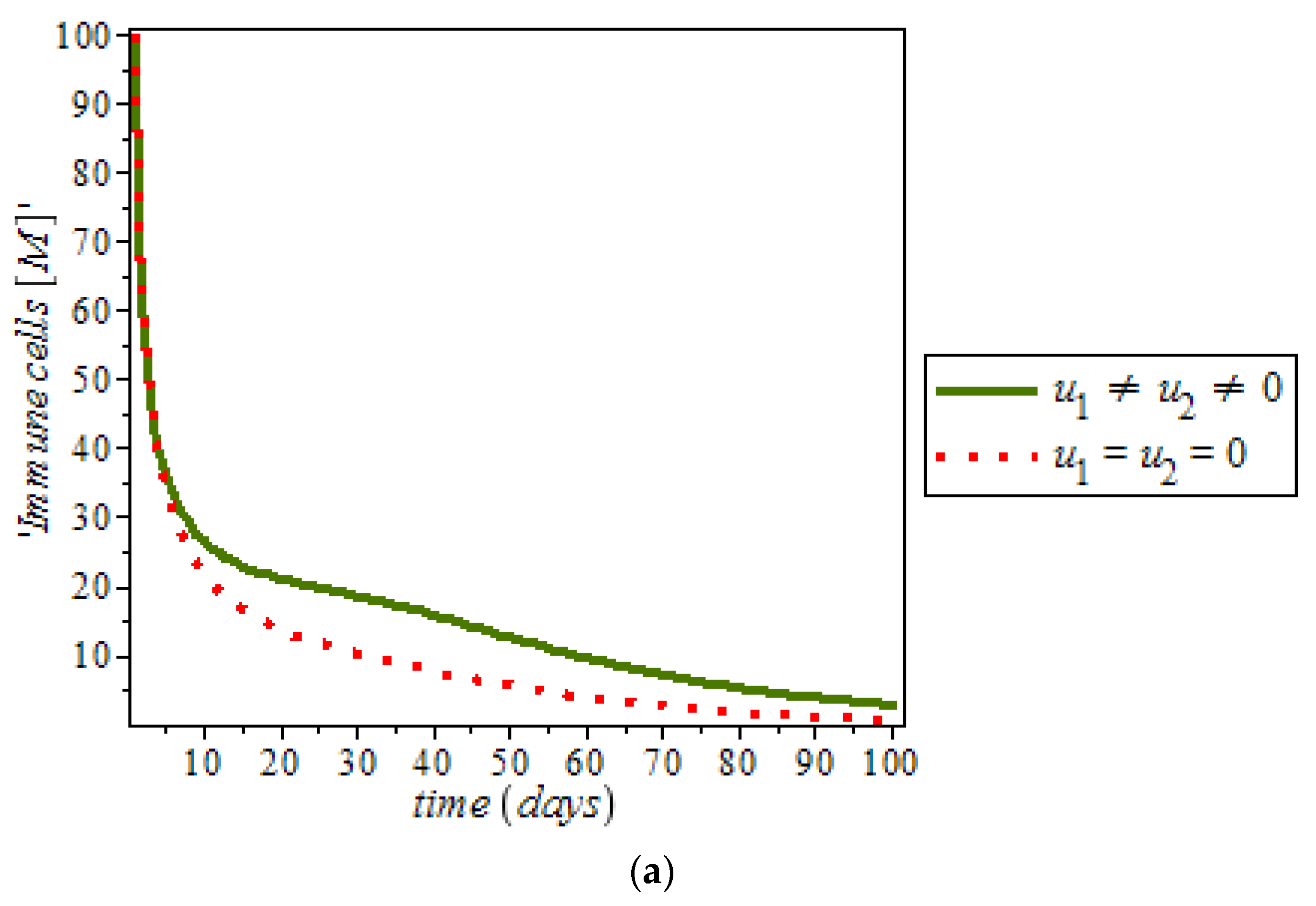In addition, ketosis also regulating hormonal imbalance [8,27]. 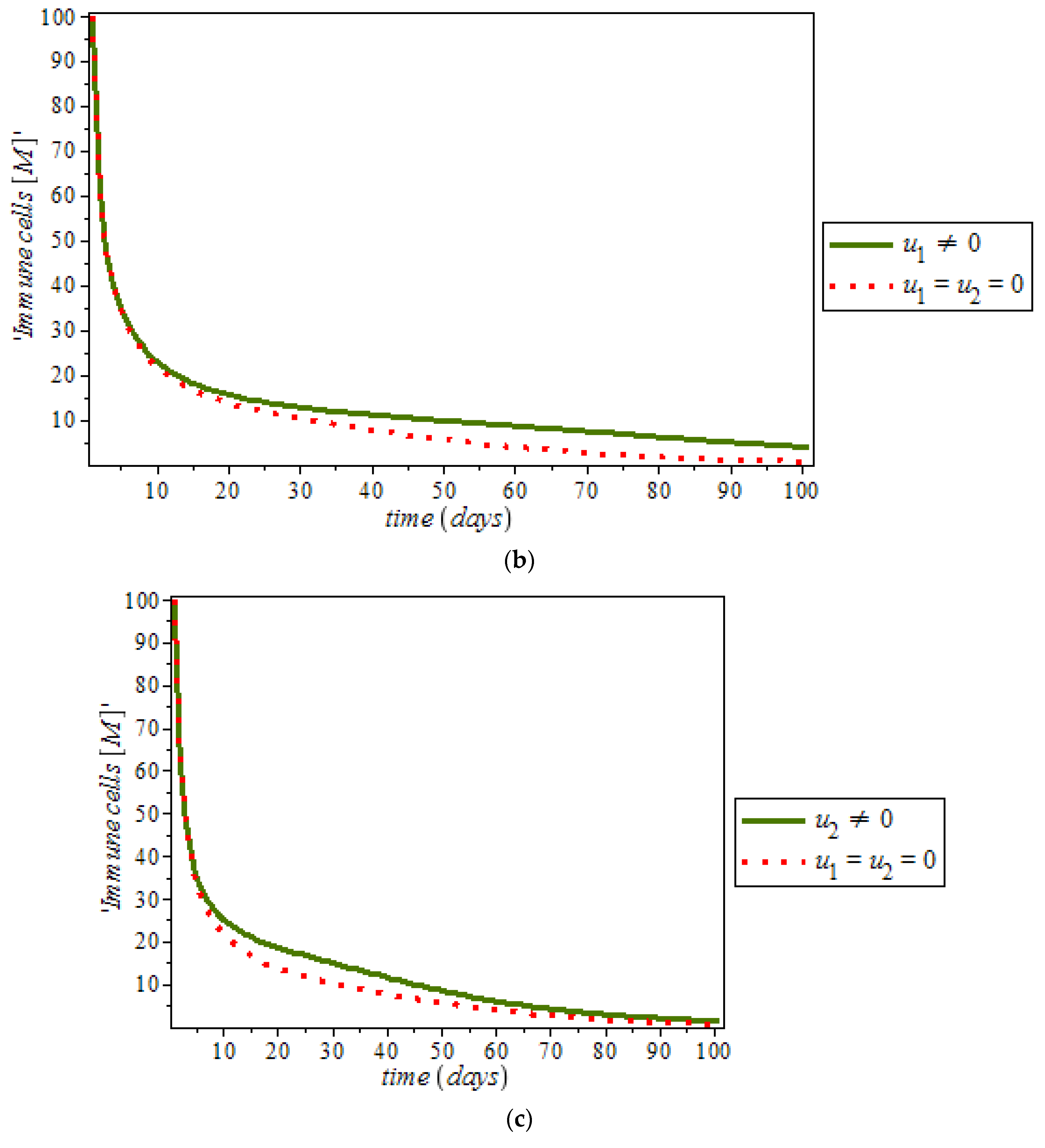On the other hand, Figure 13, shows the effect of immune response with and without controls. Immune response can help to fight cancer cells while immune system recognize cancer cells as abnormal and kill them. However, this may not be enough to eliminate cancer cells from the body.

7. Conclusions

A four-dimensional compartmental deterministic model was designed and used to monitor the dynamics of breast cancer. The existing model in [19] was extended to incorporate treatments, ketogenic diet, and an immune booster. The system (5) was rigorously analyzed to gain insight into their dynamical behaviors. The study shows the following:

• The conditions of stability of the tumor-free equilibrium (TFE) was established and the system is only local asymptotically stable (LAS) if a certain threshold quantity, known as the reproductive number, is less than unity ($R_0<1$). It implies that the number of tumor cells in the body will be brought to zero if proper treatments and a ketogenic diet that can force make the threshold to a value less than unity are monitored.
• An individual has the chance of developing breast cancer depending on the level of the immune system (s), the efficacy of the anti-cancer drug (k) and the rate at which the ketogenic diet (d) is being taken to fight tumor cells. We also found out that the presence of excess estrogen in system makes it unstable, as depicted in Figure 7. This implies that any additional estrogen quantity introduced into the body through the birth control, and hormone replacement therapy (HRT) enhances the rate of tumor formation. Thus, the development of breast cancer is certain.
• The transition from normal cells class to tumor cells class plays a crucial role in breast cancer dynamics $({\lambda }_1)$. More tumor is formed if the DNA is damaged or altered as a result of excess estrogen, which reduces the number of normal cells being produced by red blood cells.

Furthermore, the results show that tumor cell formation depend on the level of excess estrogen introduced into the body system. It must be noted that the ability to resist changes in structure and amount of estrogen released during natural biological processes is dependent on an individual’s DNA. Such biological processes include: premenopausal and menopause stages. Other risk factors may also be incorporated in the model for future work, which might generate different results.

However, the focus of this study has been identifying the advantages that come with the process of breast cancer relief policies that combined anti-cancer drugs and ketogenic diet procedures to knit the circumstances of unlimited and limited resources. The effort to moderate the effect of breast cancer on the body can be fruitful, especially if our basic reproductive number R₀ is properly analyzed. In addition, moderation is conceivable if the planning of intercessions is sufficiently quick and if the arrangement includes the utilization of more than one therapy procedure. No therapy (ketogenic diet and anti-cancer drug) is possible, unless minimal resources are accessible.

8. Further Research

Breast cancer is a health challenge disease, especially among women world-wide. This study explored the use of a quadratic control law to formulate the optimal control problem for the objective function. Hence, the authors hope to conduct further research into the application of a switching function and to investigate the side-effects of anti-cancer drugs by employing a linear control law to formulate the optimal control problem for further study.