Cost-Effective Analysis of Control Strategies to Reduce the Prevalence of Cutaneous Leishmaniasis, Based on a Mathematical Model

Abstract

Leishmaniasis is a neglected tropical vector-borne epidemic disease, and its transmission is a complex process. Zoonotic transmission to humans or animals occurs through the bites of female Phlebotominae sand flies. Here, reservoir is considered as a major source of endemic pathogen pool for disease outbreak, and the role of more than one reservoir animal becomes indispensable. To study the role of the reservoir animals on disease dynamics, a mathematical model was constructed consisting of susceptible and infected populations of humans and two types of reservoir (animal) and vector populations, respectively. Our aim is to prevent the disease by applying a control theoretic approach, when more than one type of reservoir animal exists in the region. We use drugs like sodium stibogluconate and meglumine antimoniate to control the disease for humans and spray insecticide to control the sand fly population. Similarly, drugs are applied for infected reservoir animals of Types A and B. We calculated the cost-effectiveness of all possible combinations of the intervention and control policies. One of our findings is that the most cost-effective case for Leishmania control is the spray of insecticides for infected sand fly vector. Alternate strategic cases were compared to address the critical shortcomings of single strategic cases, and a range of control strategies were estimated for effective control and economical benefit of the overall control strategy. Our findings provide the most innovative techniques available for application to the successful eradication of cutaneous leishmaniasis in the future.

1. Introduction

The disease leishmaniasis is caused by protozoan parasites from the genus Leishmania (Kinetoplastida: Trypanosomatidae) in their vertebrate hosts, including humans. Leishmaniasis is a neglected tropical disease [1] in the WHO list. Leishmania parasites are transmitted to other mammalian species through the vector bites of infected female phlebotomine sand flies [2,3]. Seventy animal species, including humans, have been found as natural reservoir hosts of Leishmania parasites [4]. Currently, the disease is endemic in eighty-eight countries [5,6]. These countries (e.g., Afghanistan, Algeria, Iran, Iraq, Pakistan, Brazil, Peru, etc.) account for more than 90% of the global cases of cutaneous leishmaniasis [7,8]. It is estimated that 12 million cases, comprising 1.5 to 2 million new cases, occur globally each year [9]. In India, Bihar and Rajasthan are the main affected states. The parasite’s life-cycle occurs alternatively between a mammalian host and insect vectors. These vectors are phlebotomine sand flies (Diptera: Psychodidae, subfamily Phlebotominae). The Leishmania parasite thrives and spends a part of its life cycle within the female sand flies. The parasites are found alternatively as flagellated, motile promastigotes in the alimentary tract of phlebotomine sand flies, or as obligate intracellular aflagellate amastigotes in the phagolysosomes of mammalian host macrophages. Outside the vertebrate host, the Leishmania life cycle is confined to the digestive tract of sand flies, which become aggressively active during the warmer months in humid environments. It is established that mammals of several orders can be infected by the Leishmania sp. Natural Leishmania infections are found in a range of non-human mammal hosts (mainly marsupials, rodents, edentates, and carnivores). Reservoir implication is difficult because it is often specific to the nature of the local domain of animal context, and it depends on many variables (e.g., host abundance and distribution, infectiousness to the sand fly vector), which are rarely investigated. Domestic animals such as dogs can serve as reservoirs for the parasite. Transmission can occur from dog to sand fly, and from sand fly to human. Another important reservoir is the rodent population, which can serve as the cryptic reservoir for the persistence of the endemic state of infection, as recently suggested by many new research works. Recent evidence suggests that increasing species richness can lower or enhance the infection rate, which must be accounted for in this endemic state of disease despite the measures taken to control it [10]. Note that the prevalence of hosts in the affected region can influence disease transmission rates. We thus have considered disease transmission by the cryptic reservoirs, which are normally beyond control program coverage. The presence of more than two reservoir animals apart from the human host can exert a significant dilution effect due to selective pressure of host preference. It is widely believed that rodents can serve as the cryptic reservoir host in both urban and rural areas where they can outnumber the domestic animal population swiftly and help in the survival of the Leishmania pathogen. Recent evidence of this has come from Tunisia [11], where rodents are a potential reservoir of Leishmania pathogens. Presently, four clinical forms for leishmaniasis exist. These are cutaneous leishmaniasis (CL), mucocutaneous leishmaniasis (known as espundia), visceral leishmaniasis (known as kala-azar), and post-kala-azar dermal leishmaniasis (PKDL) [2,12]. Transmission modes are of zoonotic and/or anthroponotic type for cutaneous leishmaniasis (CL). In anthroponotic-type transmission, the sand flies are infected by a human during a blood meal, while in zoonotic transmission cycles animals serve as potential reservoir hosts [13].

The clinical symptom of CL is painless skin ulcers. Dermal changes may appear in only one to two weeks after being bitten by the sand fly. However, sometimes symptoms will not appear for months or years. The disease starts as an erythematous papule which gradually increases in size and turns into a nodule. It ultimately ulcerates and crusts over. The edge is frequently raised and distinct [9]. These are primarily ulcers in the mouth and nose, or on the lips. Other symptoms are stuffy or runny nose, nose bleeds, asphyxia. The fundamental prevention therapy for cutaneous leishmaniasis is pentavalent antimonial compounds. Presently, oral and topical prevention management are in practice.

Leishmania amazonensis is an intracellular protozoan parasite responsible for chronic cutaneous leishmaniasis. Cutaneous leishmaniasis is often self-healing, particularly in infection with L. major and L. mexicana. Therefore, prevention is not always recommended. However, if lesions do not spontaneously heal within six months or if the lesions are especially disfiguring and in a cosmetically sensitive area, prevention is indicated. Even though lesions may heal eventually in the absence of prevention, the process is often long and produces significant scarring, thereby justifying the use of chemotherapy. The goal of preventing cutaneous leishmaniasis is twofold: the eradication of amastigotes as well as reducing the size of the lesions so that healing will take place with minimal scarring.

Mathematical models can serve as a new tool to investigate the fate of infection dynamics with a multi-host environment. However, theoretical works on this topic are very rare, motivating us to study such dynamics with two different reservoir animals, as well as human and vector populations. Bacaer et al. [14] proposed a mathematical model taking the seasonal fluctuations into account in order to formulate an age-structured model and find the basic reproduction number based on periodic backgrounds. They suggested that the epidemic could be prevented if the vector population was reduced. Chaves et al. [3] studied a mathematical model for cutaneous leishmaniasis in the Americas and found conditions for the commencement of the infection. They presented a simple model to represent the dynamics of transmission densities of infected incidental hosts, infected reservoir hosts, and infected vectors. Miller and Huppert [10] studied multiple hosts of vector-borne infectious diseases from a significant fraction of the global infectious disease burden. They explored the relationship between host diversity, vector behavior, and disease risk. They developed a new dynamic model which included two distinct host species and one vector species with variable host preferences. They discussed the role of more than one reservoir population and how it could affect the disease transmission depending on host preferences and biting intensity. Biswas et al. [15] developed different models of cutaneous leishmaniasis consisting of different aspects of the disease transmission. We have previously considered susceptible and infected human and vector populations with the target of reducing the vector population so that the disease can be controlled. Then, considering the role of the macrophage for developing the disease intracellularly, we considered another stage of infection, as there is a transformation from the promastigote stage to a mastigote stage. Finally, we modelled the application of optimal drug dose to the infected macrophage cell and parasite populations in order to control the parasite population in the macrophage cells [16]. We have also studied a model through an impulsive strategy in a fixed time interval to observe perfect drug adherence behavior. The model has been analyzed to determine the threshold time interval and minimum effectiveness of drugs and also to observe the effect of an impulsive strategy in a non-fixed time interval on the system [17]. Recently, Biswas et al. [18] developed a model for evaluating the utility of awareness in controlling cutaneous leishmaniasis in affected regions where social mass media is present.

A recent mathematical model has focused on the transmission dynamics for anthroponotic cutaneous leishmaniasis in human populations and its control [19]. However, cutaneous leishmaniasis studies involving two reservoir animals has not yet been explored in the epidemiological literature. In this article, our study was motivated by the work of Huppert [10] and Chaves [3] using a set of ordinary differential equations as the foundation of the mathematical study of cutaneous leishmaniasis with two reservoir populations. We modelled the use of drugs for the human host, therapeutics for the animal reservoir, and insecticide application for the vector population, and studied the system using an optimal control technique. The aim of the optimal control problem was to minimize infection with cumulative control strategies to exert maximum benefit to the affected hosts. We also considered different control strategies and examined the impact of different combinations of these measures in controlling the disease. We used Pontryagin’s minimum principle to derive the necessary conditions for the optimal control of the disease. By calculating the cost of drugs in each of the different strategies along with investigating the cost-effectiveness of the four control strategies under consideration, we determined the most effective strategy for eliminating leishmaniasis with minimum costs. The next section describes the formulation of the general model.

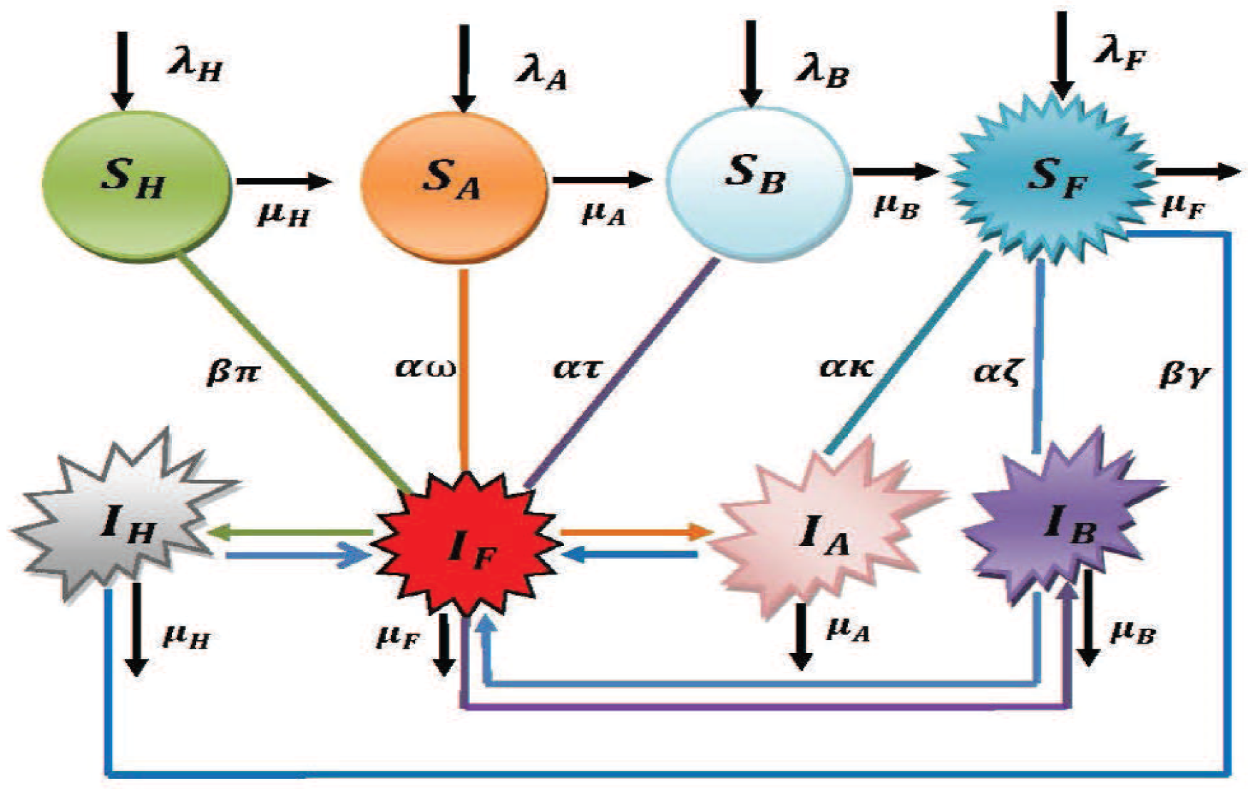
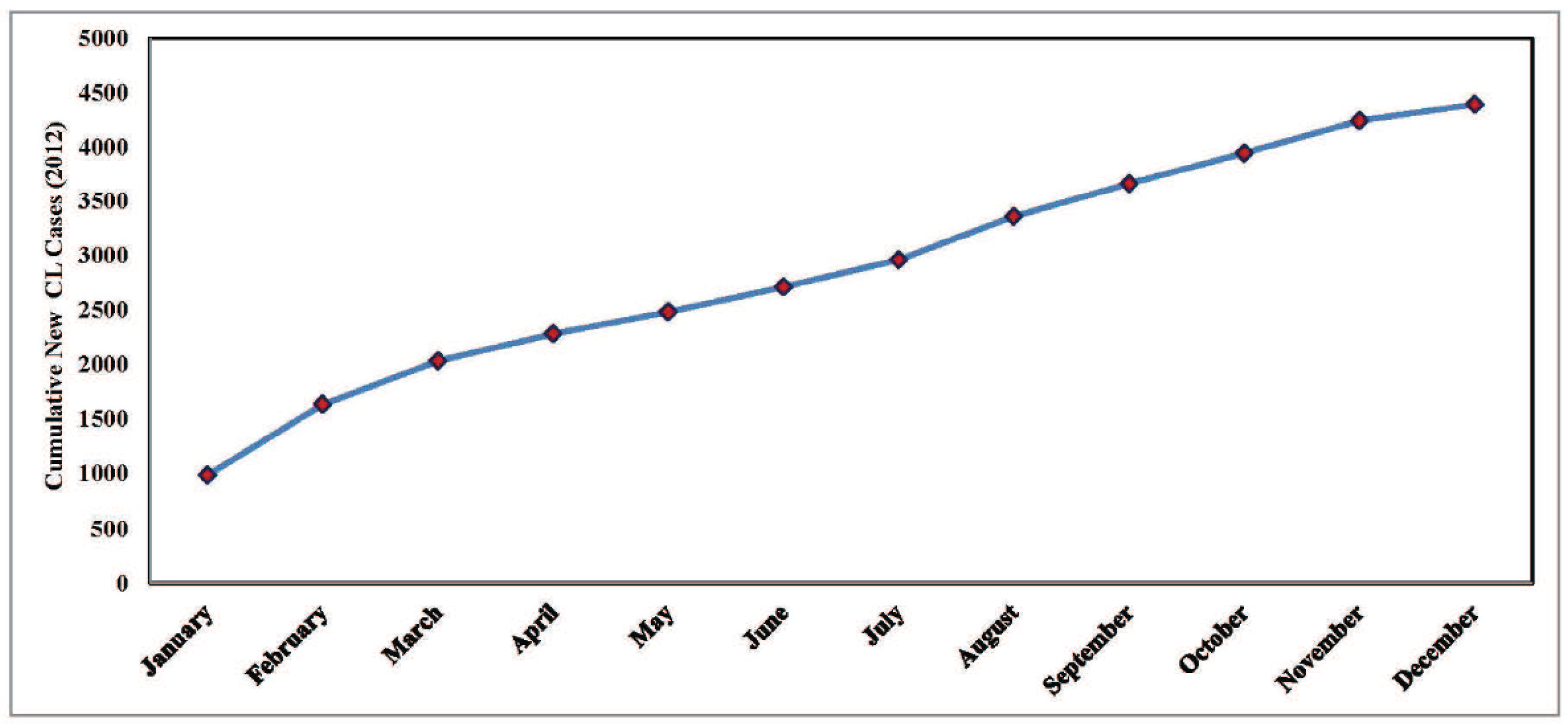
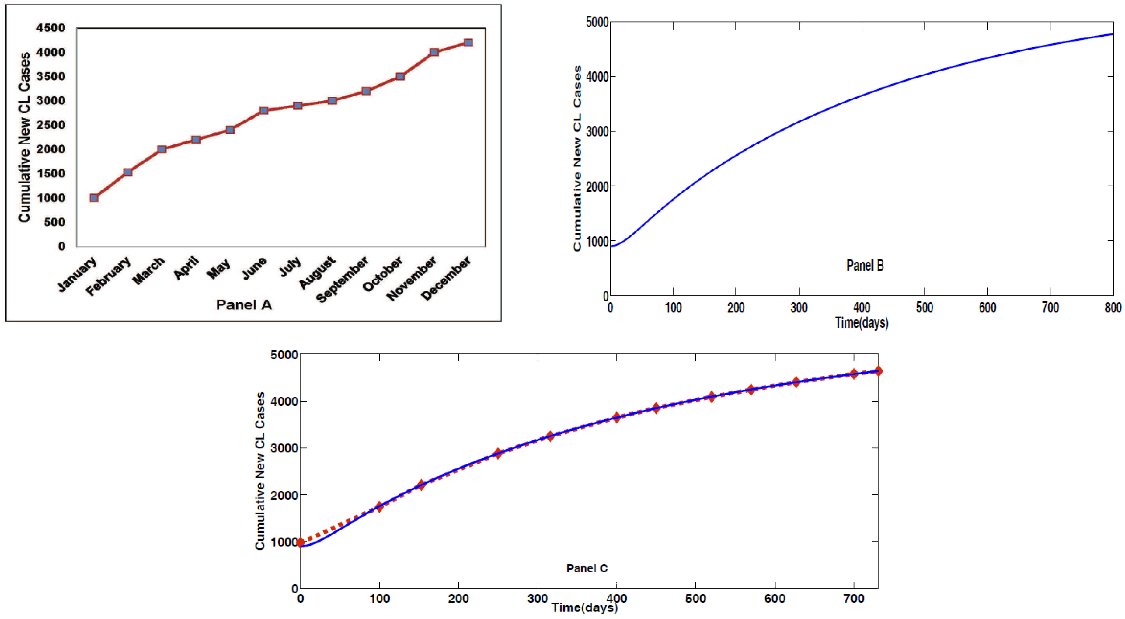
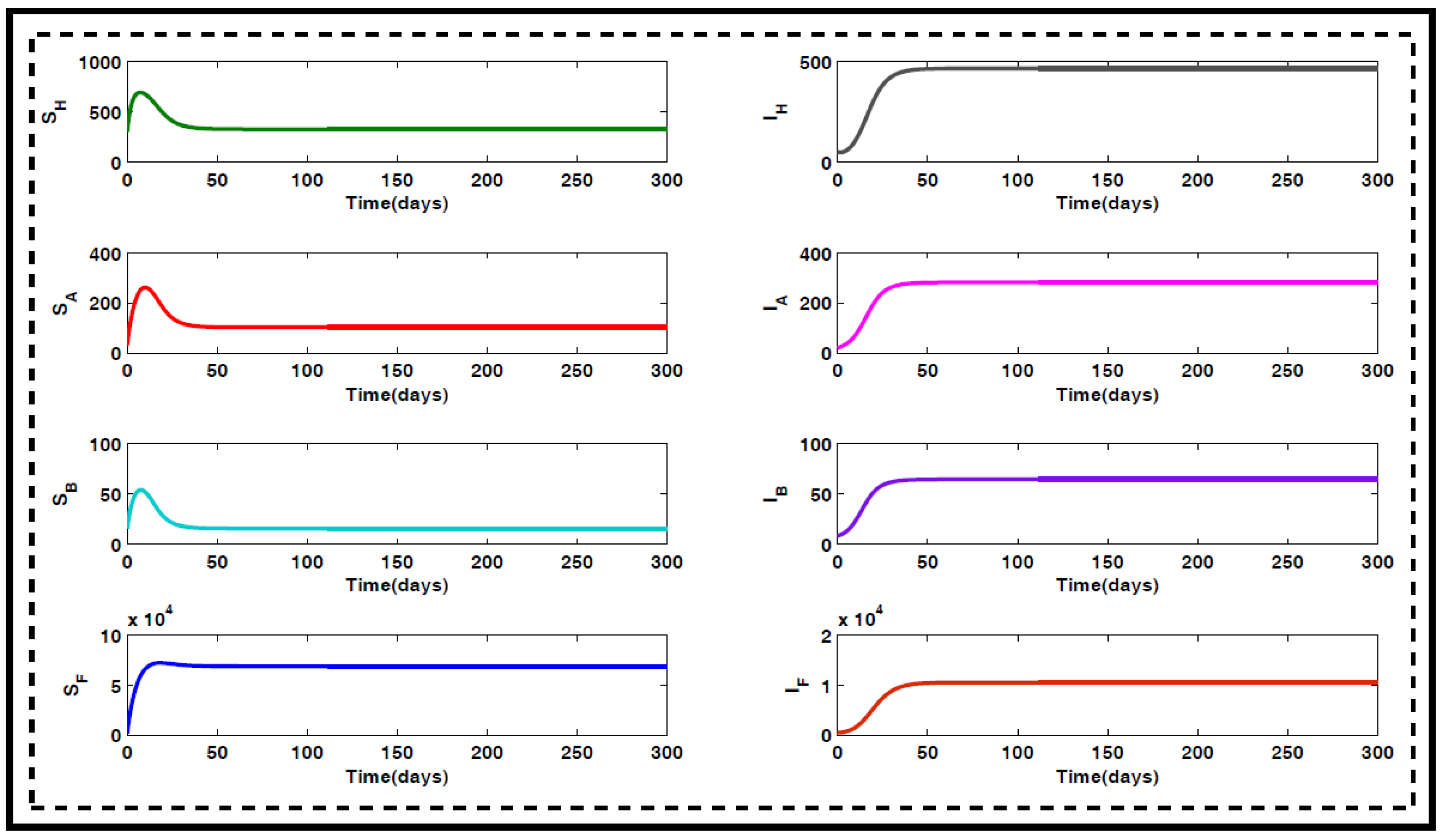
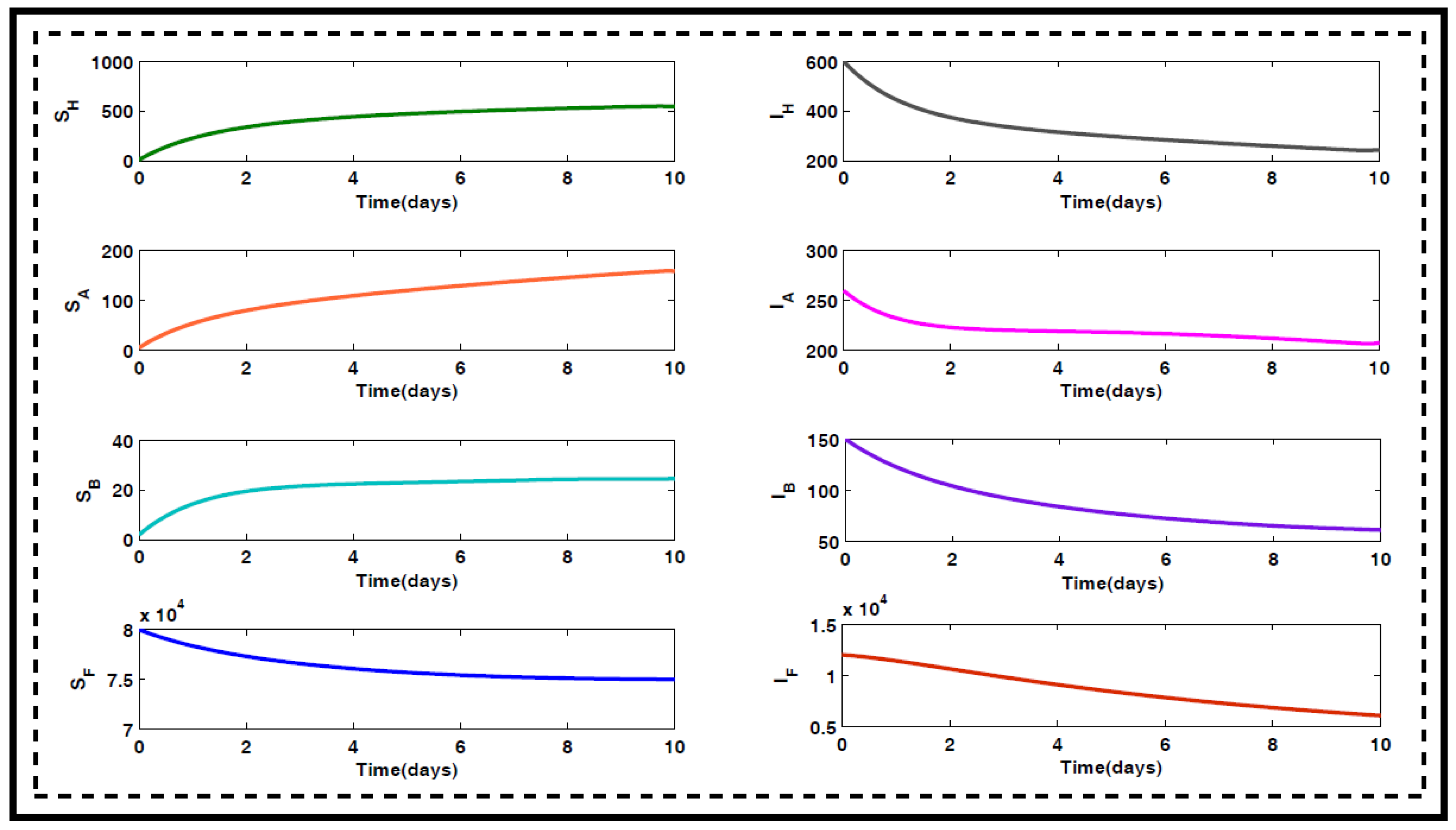
2. Model Formulation through Schematic Diagram and Its Validation

To formulate the mathematical model of cutaneous leishmaniasis, two types of animal reservoirs were considered: domestic and wild. For example, dog is the domestic animal reservoir for leishmaniasis (e.g., domestic dogs play the role of a reservoir host of Leishmania donovani in eastern Sudan), and some species of rodent (e.g., great gerbil, the crab-eating fox (Cerdocyon thous), opossums (Didelphis species), etc.) are wild animals worth consideration. Humans are in closer contact with domestic animals than they are with wild animals. We considered rodents to be cryptic reservoirs in nature, so they are away from human contact with respect to the domestic animals (e.g., dog). Furthermore, the recruitment rates and natural death rates of domestic animals and wild animals are different. For this reason, we considered two different classes of reservoirs: Type A and Type B.

We considered the transmission of the disease between four distinct populations: the human host population, Type A animals, Type B animals, and the vector population. The total human population was considered as:

$$S_H\left(t\right)+I_H\left(t\right),$$

where $S_H\left(t\right)$ denotes the susceptible individuals and $I_H\left(t\right)$ denotes the individuals infected with cutaneous leishmaniasis.

Reservoir classes are of two types. They are susceptible animals of Type A (i.e., $S_A\left(t\right)$) and susceptible animals of Type B (i.e., $S_B\left(t\right)$), and the corresponding infected classes are denoted by $I_A\left(t\right)$ and $I_B\left(t\right)$, respectively. Herein, the total reservoir population was considered as:

$$S_A\left(t\right)+I_A\left(t\right)$$

and

$$S_B\left(t\right)+I_B\left(t\right).$$

We considered the vector (sand fly) population to be of two categories: the susceptible vector population $S_F\left(t\right)$ and the infected vector population $I_F\left(t\right)$. The total vector (sand fly) population was considered as:

$$S_F\left(t\right)+I_F\left(t\right).$$

Here ${\lambda }_H$, ${\lambda }_A$, ${\lambda }_B$, and ${\lambda }_F$ are the constant recruitment rates of humans, Type A animals, Type B animals, and sand fly. ${\mu }_H$, ${\mu }_A$, ${\mu }_B$, and ${\mu }_F$ are their respective natural death rates.

For disease transmission, a susceptible human becomes infected through mass action after interaction with the infected vector, where $\beta$ is the per capita biting rate of vector on human and $\pi$ is the transmission probability per bite per human [14]. Thus, the infection term is frequency-dependent [20], and is described as:

$$\beta \pi I_F\frac{S_H}{S_H+I_H}.$$

A susceptible Type A animal ($S_A$) becomes infected by the bite (bite rate is $\alpha$) of an infected sand fly ($I_F$) with the transmission probability $\omega$. Here, the transmission of the disease is frequency-dependent [20] and is defined by:

$$\alpha \omega I_F\frac{S_A}{S_A+I_A}.$$

A susceptible Type B animal ($S_B$) becomes infected by the bite (bite rate is $\alpha$) of an infected sand fly ($I_F$) with the transmission probability $\tau$. The infection spreads as a frequency-dependent transmission [20], and is given as:

$$\alpha \tau I_F\frac{S_B}{S_B+I_B}.$$

A susceptible vector becomes infected after an interaction with an infected human at the rate $\beta$ with transmission probability $\gamma$ per bite from human to sand fly. Further, a susceptible sand fly ($S_F$) becomes infected by biting (per capita biting rate is $\alpha$) infected animals of Type A ($I_A$) and Type B ($I_B$) with the transmission probability $\kappa$ and $\zeta$, respectively. Thus, a susceptible sand fly can be infected with the accumulation term:

$$\beta \gamma S_F\frac{I_H}{S_H+I_H}+\alpha \kappa S_F\frac{I_A}{S_A+I_A}+\alpha \zeta S_F\frac{I_B}{S_B+I_B}.$$

Abubakar et al. [21] found that leishmaniasis occurrence is a seasonal phenomenon in the regions of Africa. In the region, low transmission happens in the middle of the year and high transmission occurs in September. We can take biting rate as of the form: $\beta \left(t\right)={\beta }_0(1+{\delta }_{r}sin\frac{2\pi t}{365})$. The biting rate $\beta \left(t\right)$ is based on a period of 365 days and varies with temperature. Average biting rate and amplitude of seasonality are denoted by ${\beta }_0$ and ${\delta }_r$ [22,23], respectively.

A positive dog elimination strategy reduces the source of infection and prevents more non-infected sand flies from acquiring the parasites. An infected dog prevention strategy can reduce the source of infection, but without elimination. However, preventive measures on the dog do not necessarily eliminate the parasite from the dog’s organ system. Dog vaccination does not eliminate the source of infection, but it protects the remaining susceptible dogs from becoming infected. Thus, there is a reduction in the number of infected dogs by natural elimination. The use of insecticide in impregnated dog collars works (if used by all dogs) by protecting the susceptible ones (similar to the vaccine activity) and isolating the source of infection (similar to positive dog elimination).

In nature, the prevalence of Leishmania infection in the entire sand fly population can be very low (<0.1%), even in areas of endemicity and high transmission. As a consequence, if the replacement of parasite is accelerated, there is not enough time for the parasite to mature inside the sand fly. Therefore, we do not consider the latent status in our model [24,25].

The dynamics of the disease in humans and sand flies and two reservoir (animal) populations are described in Figure 1. From the above description, we can construct the following system of differential equations in the form given below:

$$\begin{array}{ccc}\hfill {\dot{S}}_H& =& {\lambda }_H-\beta \pi I_F\frac{S_H}{S_H+I_H}-{\mu }_H{S}_H,\hfill \\ \hfill {\dot{I}}_H& =& \beta \pi I_F\frac{S_H}{S_H+I_H}-{\mu }_H{I}_H,\hfill \\ \hfill {\dot{S}}_A& =& {\lambda }_A-\alpha \omega I_F\frac{S_A}{S_A+I_A}-{\mu }_A{S}_A,\hfill \\ \hfill {\dot{I}}_A& =& \alpha \omega I_F\frac{S_A}{S_A+I_A}-{\mu }_A{I}_A,\hfill \\ \hfill {\dot{S}}_B& =& {\lambda }_B-\alpha \tau I_F\frac{S_B}{S_B+I_B}-{\mu }_B{S}_B,\hfill \\ \hfill {\dot{I}}_B& =& \alpha \tau I_F\frac{S_B}{S_B+I_B}-{\mu }_B{I}_B,\hfill \\ \hfill {\dot{S}}_F& =& {\lambda }_F-\beta \gamma S_F\frac{I_H}{S_H+I_H}-\alpha \kappa S_F\frac{I_A}{S_A+I_A}-\alpha \zeta S_F\frac{I_B}{S_B+I_B}-{\mu }_F{S}_F,\hfill \\ \hfill {\dot{I}}_F& =& \beta \gamma S_F\frac{I_H}{S_H+I_H}+\alpha \kappa S_F\frac{I_A}{S_A+I_A}+\alpha \zeta S_F\frac{I_B}{S_B+I_B}-{\mu }_F{I}_F,\hfill \end{array}$$

(1)

which satisfies the conditions $S_H+I_H>0$, $S_A+I_A>0$, $S_B+I_B>0$, and $S_F+I_F>0$.

2.1. Properties of the Model

All parameters of the model (1) are non-negative. Moreover, as the discussed model actually describes a living population, we assume the state variables to be non-negative at time $t=0$.

Note that the total human population size, $S_H+I_H\to \frac{{\lambda }_H}{{\mu }_H}$, reservoir population size, $S_A+I_A\to \frac{{\lambda }_A}{{\mu }_A}$ and $S_B+I_B\to \frac{{\lambda }_B}{{\mu }_B}$ and $S_F+I_F\to \frac{{\lambda }_F}{{\mu }_F}$ as $t\to \infty$. It follows that the probable region is represented by: $\mathfrak{D}=\{(S_H,I_H,S_A,I_A,S_B,I_B,S_F,I_F)\in {\mathbb{R}}_{+}^8:S_H,I_H,S_A,I_A,S_B,I_B,S_F,I_F\ge 0$, $S_H+I_H\le \frac{{\lambda }_H}{{\mu }_H}$, $S_F+I_F\le \frac{{\lambda }_F}{{\mu }_F}$, $S_A+I_A\le \frac{{\lambda }_A}{{\mu }_A}$ and $S_B+I_B\le \frac{{\lambda }_B}{{\mu }_B}$}, a positive invariant region. Hence, the model is mathematically efficient and proves to be adequate in estimating the dynamics of the model in the positive invariant domain $\mathfrak{D}$. Here ${\mathbb{R}}_{+}^8$ denotes the non-negative space of ${\mathbb{R}}^8$, where we specify $\overline{\mathfrak{D}}$ and $\partial \mathfrak{D}$ to represent the boundary and the interior region of $\mathfrak{D}$, respectively.

We take the ratio between female sand fly vectors and humans as:

$$a=\frac{S_F+I_F}{S_H+I_H},\mathrm{the}\mathrm{number}\mathrm{of}\mathrm{female}\mathrm{sandflies}\mathrm{per}\mathrm{human}\mathrm{host}.$$

Here, a is constant because the population density of the host does not affect the number of blood meals taken by a vector per unit time.

In either case, we take the ratio between female sand fly (vector) and reservoir as:

$$b=\frac{S_F+I_F}{S_A+I_A}\mathrm{and}c=\frac{S_F+I_F}{S_B+I_B}.$$

The parameters used in our model actually represent the infected cases of leishmaniasis in South Sudan in the year 2012 [21]. In Figure 2, the data show a maximum prevalence in January–February. After that, fewer cases occured than in previous months. Figure 3 shows that the total number of leishmaniasis incidents for the year 2012 and the estimated model parameter values were almost fitted with same line. The fitted model was further used to perform simulations which would serve as a predictive tool for future cases of leishmaniasis for the forthcoming year (i.e., January to December, 2013). Our model successfully predicted that, cumulatively, 3000 and 4770 new cases of leishmaniasis were to be recorded during the beginning of January 2013 and the end of December 2013, respectively. Hence, for the forthcoming year 2013, approximately 1770 new cases of leishmaniasis were predicted. Our estimated model parameter values (

Table 1. List of parameters.

Parameter	Definition	Range	Default Value	Reference
${\lambda }_H$	Recruitment rate of human population	300–318	317	[5]
${\lambda }_F$	Recruitment rate of sand fly population	14,950–15,000	14,950	[5]
${\lambda }_A$	Recruitment rate of animal population of Type A	70–150	73	[5]
${\lambda }_B$	Recruitment rate of animal population of Type B	3–40	20	[32]
${\mu }_H$	Death rate of human population	0.000007–0.0001	0.00004	$Assumed$
${\mu }_F$	Death rate of sand fly population	0.188–0.795	0.189	[5]
${\mu }_A$	Death rate of animal population of Type A	0.06–0.21	0.19	[5]
${\mu }_B$	Death rate of animal population of Type B	0.089–0.255	0.25	[32]
$\beta$	Biting rate of sand fly on human	0.15–0.29	0.24	[5,9]
$\alpha$	Biting rate of sand fly on animals of Type A and Type B	0.15–0.25	0.16	[5]
$\pi$	Transmission probability of CL in sand fly	0.12–0.24	0.18	[5,9]
$\omega$	Transmission probability of CL on animal of Type A	0.11–0.172	0.12	[32]
$\tau$	Transmission probability of CL on animal of Type B	0.02–0.071428	0.05	[5,9]
$\gamma$	Transmission probability of CL in sand fly from infected human	0.11–0.25	0.14	[5,9]
$\kappa$	Transmission probability of CL in sand fly from infected animal A	0.07–0.21	13	[5,9]
$\zeta$	Transmission probability of CL in sand fly from infected animal B	0.04–0.21	0.12	[32]

) coincided with the real data values. Thus, the initial human demographic parameters $S_H\left(0\right)$, $I_H\left(0\right)$ along with the initially infected reservoir population $S_A\left(0\right)$, $I_A\left(0\right)$, $S_B\left(0\right)$, $I_B\left(0\right)$ and sand fly population $S_F\left(0\right)$, $I_F\left(0\right)$ were estimated. Additionally, $\pi$, $\omega$, and $\tau$ are disease transmission probability in humans and Type A and B reservoirs, respectively.

From the model (1), the number of new CL cases ${I_H}_c$ (infected human) can be written as:

$$\begin{array}{ccc}\hfill \frac{d{I_H}_c}{dt}& =& \beta \pi I_F\frac{S_H}{S_H+I_H}.\hfill \end{array}$$

(2)

This represents the rate of increase of the number of new CL occurrences, where $\pi$ is the transmission probability of the disease in humans, and $\beta$ is the biting rate of sand fly on humans.

2.2. Existence Condition

The system (1) has two equilibrium points, one of which is disease-free equilibrium $E_0(\frac{{\lambda }_H}{{\mu }_H},0,\frac{{\lambda }_A}{{\mu }_A},0,\frac{{\lambda }_B}{{\mu }_B},0,\frac{{\lambda }_F}{{\mu }_F},0)$ and the other is endemic equilibrium $E^{*}(S_H^{*},I_H^{*},S_A^{*},I_A^{*},S_B^{*},I_B^{*},S_F^{*},I_F^{*})$, where $S_H^{*}=\frac{{\lambda }_H-{\mu }_H{I}_H^{*}}{{\mu }_H},$ $S_A^{*}=\frac{{\lambda }_A-{\mu }_A{I}_A^{*}}{{\mu }_A},$ $S_B^{*}=\frac{{\lambda }_B-{\mu }_B{I}_B^{*}}{{\mu }_B},$ $S_F^{*}=\frac{{\lambda }_F}{\frac{{\beta }^2\pi \gamma I_F^{*}}{(\beta \pi I_F^{*}+{\lambda }_H)}+\frac{{\alpha }^2\kappa \omega I_F^{*}}{(\alpha \omega I_F^{*}+{\lambda }_A)}+\frac{{\alpha }^2\zeta \tau I_F^{*}}{(\alpha \tau I_F^{*}+{\lambda }_B)}+{\mu }_F},$ $I_H^{*}=\frac{{\lambda }_H\beta \pi I_F^{*}}{(\beta \pi I_F^{*}+{\lambda }_H){\mu }_H},$ $I_A^{*}=\frac{\alpha \omega {\lambda }_A{I}_F^{*}}{(\alpha \omega I_F^{*}+{\lambda }_A){\mu }_A},$ $I_B^{*}=\frac{{\lambda }_B\alpha \tau I_F^{*}}{(\alpha \tau I_F^{*}+{\lambda }_B){\mu }_B}$ and $I_F^{*}$ are determined from the equation $A_1{I_F^{*}}^3+B_1{I_F^{*}}^2+C_1{I}_F^{*}+D_1=0$, where

• $A_1=\left((a_1{b}_3{c}_3+b_1{a}_3{c}_3+c_1{a}_3{b}_3)(d_1-d_2)-{d_2}^2{a}_3{b}_3{c}_3\right),$
• $B_1=\left(\left(a_1(b_2{c}_3+b_3{c}_2)+b_1(a_2{c}_3+a_3{c}_2)+c_1(a_2{b}_3+b_3{a}_2)\right)(d_1-d_2)-{d_2}^2(a_2{b}_3{c}_3+b_2{c}_3{a}_3+c_2{a}_3{b}_3)\right),$
• $C_1=\left((a_1{b}_2{c}_2+b_1{c}_2{a}_2+c_1{a}_2{b}_2)(d_1-d_2)-{d_2}^2(a_2{b}_2{c}_3+a_2{b}_3{c}_2+a_3{b}_2{c}_2)\right),$
• $D_1=-{d_2}^2{a}_2{b}_2{c}_2$ and
• $a_1={\beta }^2\pi \gamma ,a_2={\lambda }_H,a_3=\beta \pi ,b_1={\alpha }^2\omega \kappa ,b_2={\lambda }_A,b_3=\alpha \omega ,$
• $c_1={\alpha }^2\zeta \tau ,c_2={\lambda }_B,c_3=\alpha \tau ,d_1={\lambda }_F,d_2={\mu }_F.$

Then, the endemic equilibrium $E^{*}$ exists if ${\beta }^2\pi \gamma {\lambda }_A{\lambda }_B+{\alpha }^2\kappa \omega {\lambda }_H{\lambda }_B+{\alpha }^2\zeta \tau {\lambda }_A{\lambda }_H>\frac{{\mu }_F^2{\lambda }_A{\lambda }_B{\lambda }_H}{{\lambda }_F}$. Biological Interpretation: If the biting rate of the sand fly and transmission probabilities between infected human to vector, infected sand fly to human, infected animal to vector, and infected sand fly to animal are higher, then the system moves to its endemic state and disease persists.

2.3. Analytical Study of the Formulated Model

To find the basic reproduction ratio, four compartments ${I_H}^{\prime },{I_A}^{\prime },{I_B}^{\prime },and{i_F}^{\prime }$ were considered here. We have

$$\left[\begin{array}{c}{I_H}^{\prime }\\ {I_A}^{\prime }\\ {I_B}^{\prime }\\ {I_F}^{\prime }\end{array}\right]=\left[\begin{array}{cccc}-{\mu }_H& 0& 0& \frac{\beta \pi S_H}{S_H+I_H}\\ 0& -{\mu }_A& 0& \frac{\alpha \omega S_A}{S_A+I_A}\\ 0& 0& -{\mu }_B& \frac{\alpha \tau S_B}{S_B+I_B}\\ \frac{\beta \gamma S_F}{S_H+I_H}& \frac{\alpha \kappa S_F}{S_A+I_A}& \frac{\alpha \zeta S_F}{S_B+I_B}& -{\mu }_F\end{array}\right]\left[\begin{array}{c}{I}_H\\ I_A\\ I_B\\ I_F\end{array}\right].$$

(3)

According to [26], the above square matrix can be re-written as the subtraction of two matrices. Thus, above matrix can be expressed as $Z^{\prime }=(F-V)Z$. Here F is a non-negative matrix that contains the elements related to the generation of new infections and V is a diagonal non-negative matrix which contains the elements related to the loss of infections. F corresponds to the infectivity function of an infected population, and $V^{-1}$ is a diagonal matrix indicating the loss of an infected population. At the disease-free equilibrium point, ($\overline{S_H}=\frac{{\lambda }_H}{{\mu }_H},\overline{I_H}=0,\overline{S_A}=\frac{{\lambda }_A}{{\mu }_A},\overline{I_A}=0,\overline{S_B}=\frac{{\lambda }_B}{{\mu }_B},\overline{I_B}=0,\overline{S_F}=\frac{{\lambda }_F}{{\mu }_F},\overline{I_F}=0$), the matrix NGO (next generation operator) is NGO = $F{V}^{-1},$ where

$$F=\left(\begin{array}{cccc}0& 0& 0& \frac{\beta \pi \overline{S_H}}{\overline{S_H}+\overline{I_H}}\\ 0& 0& 0& \frac{\alpha \omega \overline{S_A}}{\overline{S_A}+\overline{I_A}}\\ 0& 0& 0& \frac{\alpha \tau \overline{S_B}}{\overline{S_B}+\overline{I_B}}\\ \frac{\beta \gamma \overline{S_F}}{\overline{S_H}+\overline{I_H}}& \frac{\alpha \kappa \overline{S_F}}{\overline{S_A}+\overline{I_A}}& \frac{\alpha \zeta \overline{S_F}}{\overline{S_B}+\overline{I_B}}& 0\end{array}\right)$$

and

$$V=\left(\begin{array}{cccc}{\mu }_H& 0& 0& 0\\ 0& {\mu }_A& 0& 0\\ 0& 0& {\mu }_B& 0\\ 0& 0& 0& {\mu }_F\end{array}\right).$$

This leads to

$$F{V}^{-1}=\left(\begin{array}{cccc}0& 0& 0& \frac{\beta \pi }{{\mu }_F}\\ 0& 0& 0& \frac{\alpha \omega }{{\mu }_F}\\ 0& 0& 0& \frac{\alpha \tau }{{\mu }_F}\\ \frac{\beta \gamma {\lambda }_F}{{\lambda }_H{\mu }_F}& \frac{\alpha \kappa {\lambda }_F}{{\lambda }_A{\mu }_F}& \frac{\alpha \zeta {\lambda }_F}{{\lambda }_B{\mu }_F}& 0\end{array}\right).$$

From the above matrix, we can calculate the basic reproduction ratio from

$$det(\mathbf{NGO}-\xi I)=0.$$

The basic reproduction ratio is the dominant eigenvalue of the matrix. It follows that the corresponding basic reproduction number is ($R_0$) = $\frac{{\lambda }_F({\alpha }^2\tau \zeta {\lambda }_A{\lambda }_H+{\alpha }^2\kappa \omega {\lambda }_H{\lambda }_B+{\beta }^2\gamma \pi {\lambda }_B{\lambda }_A)}{{{\mu }_F}^2{\lambda }_H{\lambda }_A{\lambda }_B}$. Thus, if $R_0<1$, then the system is stable at disease-free equilibrium, while if $R_0>1$, the system is unstable at disease-free states and an endemic equilibrium state exists.

The calculation of disease-free equilibrium and its stability analysis, the mathematical description of basic reproduction number ($R_0$), and the existence and permanence of the endemic solution are discussed in Figure S1 in the Supplementary Materials.

By applying Routh–Hurwitz criteria, the system is stable around the endemic equilibrium point $E^{*}(S_H^{*},I_H^{*},S_A^{*},I_A^{*},S_B^{*},I_B^{*},S_F^{*},I_F^{*})$.

3. Control Theoretic Approach for the Proposed Model

To control the disease in humans, wemodelled the use of the drugs sodium stibogluconate and meglumine antimoniate. To control the sand fly population, we modelled insecticide spraying. Additionally, we modelled the application of curative drugs to the infected Types A and B reservoir animals. These therapies, applied to infected human, animal, and vector populations, can limit the disease prevalence. Therefore, we prefer our control set quantifiable functions, defined on $[t_{start};t_{final}]$, with the constraints $0\le u_i\left(t\right)\le 1$, $i=1,2,\dots ,4$. We did not consider the side effects. We only considered the preventive case. The prevention phase is predetermined in any preventive situation. Thus, we introduce the optimal control schedule as:

(i)

The control variable $u_1$ acts as a prevention of human infection using drugs and the use of insecticide-treated bed nets to reduce infection.

(ii)

The control variable $u_2$ represents the use of medicines for the prevention of an infected reservoir population of Type A.

(iii)

The control variable $u_3$ represents the use of effective medicines for the prevention of an infected reservoir population of Type B.

(iv)

The control variable $u_4$ corresponds to measures like spraying insecticide on residences and other places where sand flies can breed and live in order to kill them at all stages.

The parameters $u_1$, $u_2$, and $u_3$ reduce the transmission rate from sandflies to humans and animals of Type A and Type B. Therefore, the approach acts as a preventative method instead of as a treatment. Here the prevention of infectious humans and reservoir hosts and the reduction of vectors is possible either by taking medication that reduces the probability of the host getting infected (e.g., either a pill or a vaccine), or via the reduction of transmission by reducing the sand fly biting rate through behavior, such as less contact between sand fly vectors and people (netting, or reducing contact, application of repellent, etc.).

The most commonly used CL prevention techniques for infected host are the use of drugs, insecticide-treated bed nets, and insecticide spraying to reduce the sand fly population. Initially, each control strategy case and its effect on CL was observed separately. Figure S2 shows the effects of different cases of control strategies in comparison with no control for each population.

The aim is to reduce the rate of infection by introducing drug administration and insecticide spraying into the system. Here the levels of $u_1\left(t\right),u_2\left(t\right),u_3\left(t\right)$, and $u_4\left(t\right)$ are considered as the proper doses of drug and insecticide spraying in the system. There is a possibility of infection upon interaction between human and vector, as well as between reservoir and vector. Thus, in this circumstance, the infected human host and animal (reservoir) population are selected for drug application, and the vector population is selected for insecticide application. The control parameters $u_1\left(t\right)$, $u_2\left(t\right)$, $u_3\left(t\right)$, and $u_4\left(t\right)$ are introduced in the dynamical model system (1). We also consider that ${\eta }_1,{\eta }_2,{\eta }_3$, and ${\eta }_4$ are the efficacy of interventions applied in human, animal, and vector, respectively. Thus, the state system reduces to:

$$\begin{array}{ccc}\hfill {\dot{S}}_H& =& {\lambda }_H-\beta (1-{\eta }_1{u}_1\left(t\right))\pi I_F\frac{S_H}{S_H+I_H}-{\mu }_H{S}_H,\hfill \\ \hfill {\dot{I}}_H& =& \beta (1-{\eta }_1{u}_1\left(t\right))\pi I_F\frac{S_H}{S_H+I_H}-{\mu }_H{I}_H,\hfill \\ \hfill {\dot{S}}_A& =& {\lambda }_A-\alpha (1-{\eta }_2{u}_2\left(t\right))\omega I_F\frac{S_A}{S_A+I_A}-{\mu }_A{S}_A,\hfill \\ \hfill {\dot{I}}_A& =& \alpha (1-{\eta }_2{u}_2\left(t\right))\omega I_F\frac{S_A}{S_A+I_A}-{\mu }_A{I}_A,\hfill \\ \hfill {\dot{S}}_B& =& {\lambda }_B-\alpha (1-{\eta }_3{u}_3\left(t\right))\tau I_F\frac{S_B}{S_B+I_B}-{\mu }_B{S}_B,\hfill \\ \hfill {\dot{I}}_B& =& \alpha (1-{\eta }_3{u}_3\left(t\right))\tau I_F\frac{S_B}{S_B+I_B}-{\mu }_B{I}_B,\hfill \\ \hfill {\dot{S}}_F& =& {\lambda }_F-\beta (1-{\eta }_4{u}_4\left(t\right))\gamma S_F\frac{I_H}{S_H+I_H}-\alpha (1-{\eta }_4{u}_4\left(t\right))\kappa S_F\frac{I_A}{S_A+I_A}\hfill \\ & & -\alpha (1-{\eta }_4{u}_4\left(t\right))\zeta S_F\frac{I_B}{S_B+I_B}-({\mu }_F+{\mu }_1)S_F,\hfill \\ \hfill {\dot{I}}_F& =& \beta (1-{\mu }_4{u}_4\left(t\right))\gamma S_F\frac{I_H}{S_H+I_H}+\alpha (1-{\eta }_4{u}_4\left(t\right))\kappa S_F\frac{I_A}{S_A+I_A}\hfill \\ & & +\alpha (1-{\eta }_4{u}_4\left(t\right))\zeta S_F\frac{I_B}{S_B+I_B}-({\mu }_F+{\mu }_1)I_F.\hfill \end{array}$$

(4)

Note that ${\mu }_1$ is the death rate of vector due to insecticide spraying, and $({\mu }_F+{\mu }_1)$ is expressed as ${\overline{\mu }}_F$.

Endemic equilibrium with control are described in the following manner: $S_H^{*}=\frac{{\lambda }_H-{\mu }_H{I}_H^{*}}{{\mu }_H}$, $S_A^{*}=\frac{{\lambda }_A-{\mu }_A{I}_A^{*}}{{\mu }_A}$, $S_B^{*}=\frac{{\lambda }_B-{\mu }_B{I}_B^{*}}{{\mu }_B}$, $S_F^{*}=\frac{{\lambda }_F}{\frac{{\beta }^2(1-{\eta }_1{u}_1)(1-{\eta }_4{u}_4)\pi \gamma I_F^{*}}{(\beta (1-{\eta }_1{u}_1)\pi I_F^{*}+{\lambda }_H)}+\frac{{\alpha }^2(1-{\eta }_2{u}_2)(1-{\eta }_4{u}_4)\kappa \omega I_F^{*}}{(\alpha (1-{\eta }_2{u}_2)\omega I_F^{*}+{\lambda }_A)}+\frac{{\alpha }^2(1-{\eta }_3{u}_3)(1-{\eta }_4{u}_4)\zeta \tau I_F^{*}}{(\alpha (1-{\eta }_3{u}_3)\tau I_F^{*}+{\lambda }_B)}+\overline{{\mu }_F}}$, $I_H^{*}=\frac{{\lambda }_H\beta (1-{\eta }_1{u}_1)\pi I_F^{*}}{(\beta (1-{\eta }_1{u}_1)\pi I_F^{*}+{\lambda }_H){\mu }_H}$, $I_A^{*}=\frac{\alpha (1-{\eta }_2{u}_2)\omega {\lambda }_A{I}_F^{*}}{(\alpha (1-{\eta }_2{u}_2)\omega I_F^{*}+{\lambda }_A){\mu }_A}$, $I_B^{*}=\frac{{\lambda }_B\alpha (1-{\eta }_3{u}_3)\tau I_F^{*}}{(\alpha (1-{\eta }_3{u}_3)\tau I_F^{*}+{\lambda }_B){\mu }_B}$, and $I_F^{*}$ is determined from the equation $A_2{I_F^{*}}^3+B_2{I_F^{*}}^2+C_2{I}_F^{*}+D_2=0$, where

$A_2=\left((a_1^{\prime }{b}_3^{\prime }{c}_3^{\prime }+b_1^{\prime }{a}_3^{\prime }{c}_3^{\prime }+c_1^{\prime }{a}_3^{\prime }{b}_3^{\prime })(d_1^{\prime }-d_2^{\prime })-{d_2^{\prime }}^2{a}_3^{\prime }{b}_3^{\prime }{c}_3^{\prime }\right),$

$B_2=\left(\left(a_1^{\prime }(b_2^{\prime }{c}_3^{\prime }+b_3^{\prime }{c}_2^{\prime })+b_1^{\prime }(a_2^{\prime }{c}_3^{\prime }+a_3^{\prime }{c}_2^{\prime })+c_1^{\prime }(a_2^{\prime }{b}_3^{\prime }+b_3^{\prime }{a}_2^{\prime })\right)(d_1^{\prime }-d_2^{\prime })-{d_2^{\prime }}^2(a_2^{\prime }{b}_3^{\prime }{c}_3^{\prime }+b_2^{\prime }{c}_3^{\prime }{a}_3^{\prime }+c_2^{\prime }{a}_3^{\prime }{b}_3^{\prime })\right),$

$C_2=\left((a_1^{\prime }{b}_2^{\prime }{c}_2^{\prime }+b_1^{\prime }{c}_2^{\prime }{a}_2^{\prime }+c_1^{\prime }{a}_2^{\prime }{b}_2^{\prime })(d_1^{\prime }-d_2^{\prime })-{d_2^{\prime }}^2(a_2^{\prime }{b}_2^{\prime }{c}_3^{\prime }+a_2^{\prime }{b}_3^{\prime }{c}_2^{\prime }+a_3^{\prime }{b}_2^{\prime }{c}_2^{\prime })\right),$

$D_2=-{d_2^{\prime }}^2{a}_2^{\prime }{b}_2^{\prime }{c}_2^{\prime }$ and

$a_1^{\prime }={\beta }^2(1-{\eta }_1{u}_1)(1-{\eta }_4{u}_4)\pi \gamma ,a_2^{\prime }={\lambda }_H,a_3^{\prime }=\beta (1-{\eta }_1{u}_1)\pi ,b_1^{\prime }={\alpha }^2(1-{\eta }_2{u}_2)(1-{\eta }_4{u}_4)\omega \kappa ,$$b_2^{\prime }={\lambda }_A,b_3^{\prime }=\alpha (1-{\eta }_2{u}_2)\omega ,$

$c_1^{\prime }={\alpha }^2(1-{\eta }_3{u}_3)(1-{\eta }_4{u}_4)\zeta \tau ,c_2^{\prime }={\lambda }_B,c_3^{\prime }=\alpha (1-{\eta }_3{u}_3)\tau ,d_1^{\prime }={\lambda }_F,d_2^{\prime }={\overline{\mu }}_F.$

The basic reproduction number with control parameter can be expressed in the form:

$${\overline{R}}_0=\frac{{\lambda }_F({\alpha }^2\tau \zeta {\lambda }_A{\lambda }_H(1-{\eta }_3{u}_3)(1-{\eta }_4{u}_4)+{\alpha }^2\kappa \omega {\lambda }_H{\lambda }_B(1-{\eta }_2{u}_2)(1-{\eta }_4{u}_4)+{\beta }^2\gamma \pi {\lambda }_B{\lambda }_A(1-{\eta }_1{u}_1)(1-{\eta }_4{u}_4))}{{{\mu }_F}^2{\lambda }_H{\lambda }_A{\lambda }_B}.$$

The purpose of our optimal control approach is to minimize the infected human and reservoir populations, reduce the vector population, and minimize the cost of prevention by using the possible minimal control variables $u_1\left(t\right)$, $u_2\left(t\right)$, $u_3\left(t\right)$, and $u_4\left(t\right)$. Now, we construct the objective function:

$$\begin{array}{c}\hfill J(u_1,u_2,u_3,u_4)={\int }_{t_{start}}^{t_{final}}[{\rho }_1{I}_H\left(t\right)+{\rho }_2{I}_A\left(t\right)+{\rho }_3{I}_B\left(t\right)+{\rho }_4{S}_F\left(t\right)+{\rho }_5{I}_F\left(t\right)\\ \hfill +\frac{1}{2}(w_1{u_1}^2+w_2{u_2}^2+w_3{u_3}^2+w_4{u_4}^2)]dt.\end{array}$$

(5)

In the objective function, ${\rho }_1,{\rho }_2$, ${\rho }_3$, ${\rho }_4$, and ${\rho }_5$ represent the weight constants of the infected human, infected animal of Type A, infected animal of Type B, and vector population (susceptible and infected), respectively, and $w_1,w_2,w_3$, and $w_4$ are weight constants for the prevention of transmission to human, animals of Types A and B, and vector control, respectively. The terms $\frac{1}{2}{w}_1{u_1}^2$, $\frac{1}{2}{w}_2{u_2}^2,\frac{1}{2}{w}_3{u_3}^2$, $\frac{1}{2}{w}_4{u_4}^2$ describe the cost of disease prevention. The first control policy $u_1\left(t\right)$ comes from the prevention policy of the infected human class. The cost related with the second control $u_2\left(t\right)$ is the medication for reservoir Type A. The cost associated with the third control technique $u_3\left(t\right)$ is the prevention using drugs in reservoir Type B, and the cost associated with the fourth control strategy $u_4\left(t\right)$ arises from applying different types of pesticides or insecticide to kill sand flies at all life stages. Here we must consider that cost is proportional to the square of the corresponding control function. Thus, the objective function can be defined as:

$$J(u_1,u_2,u_3,u_4);(u_1,u_2,u_3,u_4)\in D.$$

Next, we consider the following minimization problem:

$$J(u_1,u_2,u_3,u_4)\to min;(u_1,u_2,u_3,u_4)\in D,$$

where the corresponding control set D is expressed in the form:

$$D=\{(u_1,u_2,u_3,u_4):u_i\left(t\right)\mathrm{is}\mathrm{the}\mathrm{Lebesgue}\mathrm{measurable}\mathrm{function}\mathrm{on}$$

$$[t_{start};t_{final}]\mathrm{and}0\le u_i\left(t\right)\le 1,i=1,2,3,4\}.$$

Existence of the Optimal Control

For bounded Lebesgue measurable controls and non-negative initial conditions, there exists a non-negative bounded solution of the state system [27,28]. To find the optimal solution of the system, first, we define the Lagrangian (L) of the control system (4) as:

$$L={\rho }_1{I}_H+{\rho }_2{I}_A+{\rho }_3{I}_B+{\rho }_4{S}_F+{\rho }_5{I}_F+\frac{1}{2}(w_1{u_1}^2+w_2{u_2}^2+w_3{u_3}^2+w_4{u_4}^2).$$

Theorem 1.

For the system (4) with the non-negative initial conditions, there exists an optimal control $u^{*}=(u_1^{*},u_2^{*},u_3^{*},u_4^{*})$, such that $J(u_1^{*},u_2^{*},u_3^{*},u_4^{*})=min\{j(u_1,u_2,u_3,u_4):(u_1,u_2,u_3,u_4)\in D\}$.

Proof. 

We use the result for the existence of an optimal control in [27,29] as the control variables, and the state variables are non-negative. Now, the objective function in $u_1$, $u_2$, $u_3$, and $u_4$ satisfies the condition of convexity. By definition, the control set D is convex and closed. The existence of the optimal control is confirmed by the boundedness of the solutions of the state system. Additionally, the Lagrangian, L, is convex on the control set D. This proves the existence of an optimal control. ☐

Now we apply Pontryagin’s minimal principle [30] to the control system (4). To solve the optimal control problem, we define the Hamiltonian H with the help of the Lagrangian as follows:

$$\begin{array}{ccc}\hfill H& =& L+{\lambda }_1\frac{d{S}_H}{dt}+{\lambda }_2\frac{d{I}_H}{dt}+{\lambda }_3\frac{d{S}_A}{dt}+{\lambda }_4\frac{d{I}_A}{dt}+{\lambda }_5\frac{d{S}_B}{dt}+{\lambda }_6\frac{d{I}_B}{dt}+{\lambda }_7\frac{d{S}_F}{dt}+{\lambda }_8\frac{d{I}_F}{dt}\hfill \\ & & +{\xi }_1{u}_1+{\xi }_2(1-u_1)+{\xi }_3{u}_2+{\xi }_4(1-u_2)+{\xi }_5{u}_3+{\xi }_6(1-u_3)\hfill \\ & & +{\xi }_7{u}_4+{\xi }_8(1-u_4).\hfill \end{array}$$

where ${\lambda }_j$, $j=1,2,\dots ,8$ are the adjoint variables and ${\xi }_i$, $i=1,2,\dots ,8$ are the penalty multipliers:

(i)

$u_1=0$, where ${\xi }_1\ne 0and{\xi }_2=0$ and ${\xi }_3={\xi }_4={\xi }_5={\xi }_6={\xi }_7={\xi }_8=0$ and

(ii)

$u_1=1$, where ${\xi }_1=0and{\xi }_2\ne 0$ and ${\xi }_3={\xi }_4={\xi }_5={\xi }_6={\xi }_7={\xi }_8=0$,

(i)

$u_2=0$, where ${\xi }_3\ne 0and{\xi }_4=0$ and ${\xi }_1={\xi }_2={\xi }_5={\xi }_6={\xi }_7={\xi }_8=0$ and

(ii)

$u_2=1$, where ${\xi }_3=0and{\xi }_4\ne 0$ and ${\xi }_1={\xi }_2={\xi }_5={\xi }_6={\xi }_7={\xi }_8=0$,

(i)

$u_3=0$, where ${\xi }_5\ne 0and{\xi }_6=0$ and ${\xi }_1={\xi }_2={\xi }_3={\xi }_4={\xi }_7={\xi }_8=0$ and

(ii)

$u_3=1$, where ${\xi }_5=0and{\xi }_6\ne 0$ and ${\xi }_1={\xi }_2={\xi }_3={\xi }_4={\xi }_7={\xi }_8=0$,

(i)

$u_4=0$, where ${\xi }_7\ne 0and{\xi }_8=0$ and ${\xi }_1={\xi }_2={\xi }_3={\xi }_4={\xi }_5={\xi }_6=0$ and

(ii)

$u_4=1$, where ${\xi }_7=0and{\xi }_8\ne 0$ and ${\xi }_1={\xi }_2={\xi }_3={\xi }_4={\xi }_5={\xi }_6=0$.

The corresponding adjoint equations are given by,

$$\begin{array}{ccc}\hfill \frac{d{\lambda }_1}{dt}& =& -\frac{\partial H}{\partial S_H},\frac{d{\lambda }_2}{dt}=-\frac{\partial H}{\partial I_H},\frac{d{\lambda }_3}{dt}=-\frac{\partial H}{\partial S_A},\frac{d{\lambda }_4}{dt}=-\frac{\partial H}{\partial I_A},\hfill \\ \hfill \frac{d{\lambda }_5}{dt}& =& -\frac{\partial H}{\partial S_B},\frac{d{\lambda }_6}{dt}=-\frac{\partial H}{\partial I_B},\frac{d{\lambda }_7}{dt}=-\frac{\partial H}{\partial S_F},\frac{d{\lambda }_8}{dt}=-\frac{\partial H}{\partial I_F},\hfill \end{array}$$

(6)

where

$$\begin{array}{ccc}\hfill \frac{\partial H}{\partial S_H}& =& -{\lambda }_1\left(t\right)\left(\beta (1-{\eta }_1{u}_1)\frac{\pi I_F\left(t\right)I_H\left(t\right)}{{(S_H\left(t\right)+I_H\left(t\right))}^2}+{\mu }_H\right)+{\lambda }_2\left(t\right)\left(\beta (1-{\eta }_1{u}_1)\frac{\pi I_F\left(t\right)I_H\left(t\right)}{{(S_H\left(t\right)+I_H\left(t\right))}^2}\right)\hfill \\ & & +{\lambda }_7\left(t\right)\left(\beta (1-{\eta }_4{u}_4)\frac{\gamma S_F\left(t\right)I_H\left(t\right)}{{(S_H\left(t\right)+I_H\left(t\right))}^2}\right)-{\lambda }_8\left(t\right)\left(\beta (1-{\eta }_4{u}_4)\frac{\gamma S_F\left(t\right)I_H\left(t\right)}{{(S_H\left(t\right)+I_H\left(t\right))}^2}\right),\hfill \\ \hfill \frac{\partial H}{\partial I_H}& =& {\rho }_1+{\lambda }_1\left(t\right)\left(\beta (1-{\eta }_1{u}_1)\frac{\pi I_F\left(t\right)S_H\left(t\right)}{{(S_H\left(t\right)+I_H\left(t\right))}^2}\right)-{\lambda }_2\left(t\right)\left(\beta (1-{\eta }_1{u}_1)\frac{\pi I_F\left(t\right)S_H\left(t\right)}{{(S_H\left(t\right)+I_H\left(t\right))}^2}+{\mu }_H\right)\hfill \\ & & -{\lambda }_7\left(t\right)\left(\beta (1-{\eta }_4{u}_4)\frac{\gamma S_F\left(t\right)}{{(S_H\left(t\right)+I_H\left(t\right))}^2}\right)+{\lambda }_8\left(t\right)\left(\beta (1-{\eta }_4{u}_4)\frac{\gamma S_F\left(t\right)}{{(S_H\left(t\right)+I_H\left(t\right))}^2}\right),\hfill \\ \hfill \frac{\partial H}{\partial S_A}& =& -{\lambda }_3\left(t\right)\left(\alpha (1-{\eta }_2{u}_2)\frac{\omega I_F\left(t\right)I_A\left(t\right)}{{(S_A\left(t\right)+I_A\left(t\right))}^2}+{\mu }_A\right)+{\lambda }_4\left(t\right)\left(\alpha (1-{\eta }_2{u}_2)\frac{\omega I_F\left(t\right)I_A\left(t\right)}{{(S_A\left(t\right)+I_A\left(t\right))}^2}\right)\hfill \\ & & +{\lambda }_7\left(t\right)\left(\alpha (1-{\eta }_4{u}_4)\frac{\kappa S_F\left(t\right)I_A\left(t\right)}{{(S_A\left(t\right)+I_A\left(t\right))}^2}\right)-{\lambda }_8\left(t\right)\left(\beta (1-{\eta }_4{u}_4)\frac{\kappa S_F\left(t\right)I_A\left(t\right)}{{(S_A\left(t\right)+I_A\left(t\right))}^2}\right),\hfill \\ \hfill \frac{\partial H}{\partial I_A}& =& {\rho }_2+{\lambda }_3\left(t\right)\left(\alpha (1-{\eta }_2{u}_2)\frac{\omega I_F\left(t\right)S_A\left(t\right)}{{(S_A\left(t\right)+I_A\left(t\right))}^2}\right)-{\lambda }_4\left(t\right)\left(\alpha (1-{\eta }_2{u}_2)\frac{\omega I_F\left(t\right)S_A\left(t\right)}{{(S_A\left(t\right)+I_A\left(t\right))}^2}+{\mu }_A\right)\hfill \\ & & -{\lambda }_7\left(t\right)\left(\alpha (1-{\eta }_4{u}_4)\frac{\kappa S_F\left(t\right)S_A\left(t\right)}{{(S_A\left(t\right)+I_A\left(t\right))}^2}\right)+{\lambda }_8\left(t\right)\left(\alpha (1-{\eta }_4{u}_4)\frac{\kappa S_F\left(t\right)S_A\left(t\right)}{{(S_A\left(t\right)+I_A\left(t\right))}^2}\right),\hfill \\ \hfill \frac{\partial H}{\partial S_B}& =& -{\lambda }_5\left(t\right)\left(\alpha (1-{\eta }_3{u}_3)\frac{\tau I_F\left(t\right)I_B\left(t\right)}{{(S_B\left(t\right)+I_B\left(t\right))}^2}+{\mu }_B\right)+{\lambda }_6\left(t\right)(\alpha (1-{\eta }_3{u}_3)\frac{\tau I_F\left(t\right)I_B\left(t\right)}{{(S_B\left(t\right)+I_B\left(t\right))}^2})\hfill \\ & & +{\lambda }_7\left(t\right)\left(\alpha (1-{\eta }_4{u}_4)\frac{\zeta S_F\left(t\right)I_B\left(t\right)}{{(S_B\left(t\right)+I_B\left(t\right))}^2}\right)-{\lambda }_8\left(t\right)\left(\beta (1-{\eta }_4{u}_4)\frac{\zeta S_F\left(t\right)I_B\left(t\right)}{{(S_B\left(t\right)+I_B\left(t\right))}^2}\right),\hfill \\ \hfill \frac{\partial H}{\partial I_B}& =& {\rho }_3+{\lambda }_5\left(t\right)\left(\alpha (1-{\eta }_3{u}_3)\frac{\tau I_F\left(t\right)S_B\left(t\right)}{{(S_B\left(t\right)+I_B\left(t\right))}^2}\right)-{\lambda }_6\left(t\right)(\alpha (1-{\eta }_3{u}_3)\frac{\tau I_F\left(t\right)S_B\left(t\right)}{{(S_B\left(t\right)+I_B\left(t\right))}^2}+{\mu }_B)\hfill \\ & & -{\lambda }_7\left(t\right)\left(\alpha (1-{\eta }_4{u}_4)\frac{\zeta S_F\left(t\right)S_B\left(t\right)}{{(S_B\left(t\right)+I_B\left(t\right))}^2}\right)+{\lambda }_8\left(t\right)\left(\beta (1-{\eta }_4{u}_4)\frac{\zeta S_F\left(t\right)S_B\left(t\right)}{{(S_B\left(t\right)+I_B\left(t\right))}^2}\right),\hfill \\ \hfill \frac{\partial H}{\partial S_F}& =& {\rho }_4-{\lambda }_7\left(t\right)\{\beta (1-{\eta }_4{u}_4)\frac{\gamma I_H\left(t\right)}{(S_H\left(t\right)+I_H\left(t\right))}-\alpha (1-{\eta }_4{u}_4)\frac{\kappa I_A\left(t\right)}{(S_A\left(t\right)+I_A\left(t\right))}\hfill \\ & & -\alpha (1-{\eta }_4{u}_4)\frac{\zeta I_B\left(t\right)}{(S_B\left(t\right)+I_B\left(t\right))}-{\mu }_F\}+{\lambda }_8\left(t\right)\{\beta (1-{\eta }_4{u}_4)\frac{\gamma I_H\left(t\right)}{(S_H\left(t\right)+I_H\left(t\right))}\hfill \\ & & +\alpha (1-{\eta }_4{u}_4)\frac{\kappa I_A\left(t\right)}{(S_A\left(t\right)+I_A\left(t\right))}+\alpha (1-{\eta }_4{u}_4)\frac{\zeta I_B\left(t\right)}{(S_B\left(t\right)+I_B\left(t\right))}\},\hfill \\ \hfill \frac{\partial H}{\partial I_F}& =& {\rho }_5-{\lambda }_1\left(t\right)\beta (1-{\eta }_1{u}_1)\frac{\pi S_H\left(t\right)}{(S_H\left(t\right)+I_H\left(t\right))}+{\lambda }_2\left(t\right)\beta (1-{\eta }_1{u}_1)\frac{\pi S_H\left(t\right)}{(S_H\left(t\right)+I_H\left(t\right))}\hfill \\ & & -{\lambda }_3\left(t\right)\alpha (1-{\eta }_2{u}_2)\frac{\omega S_A\left(t\right)}{(S_A\left(t\right)+I_A\left(t\right))}+{\lambda }_4\left(t\right)\alpha (1-{\eta }_2{u}_2)\frac{\omega S_A\left(t\right)}{(S_A\left(t\right)+I_A\left(t\right))}\hfill \\ & & -{\lambda }_5\left(t\right)\alpha (1-{\eta }_3{u}_3)\frac{\tau S_B\left(t\right)}{(S_B\left(t\right)+I_B\left(t\right))}+{\lambda }_6\left(t\right)\alpha (1-{\eta }_3{u}_3)\frac{\tau S_B\left(t\right)}{(S_B\left(t\right)+I_B\left(t\right))}-{\lambda }_8\left(t\right){\overline{\mu }}_F.\hfill \end{array}$$

(7)

Again, H can be written as

$$\begin{array}{ccc}\hfill H& =& \frac{1}{2}{w}_1{u_1}^2-{\lambda }_1\left(t\right)\left(1-{\eta }_1{u}_1\right)\beta \pi I_F\left(t\right)\frac{S_H\left(t\right)}{S_H\left(t\right)+I_H\left(t\right)}+{\lambda }_2\left(t\right)\left(1-{\eta }_1{u}_1\right)\beta \pi I_F\left(t\right)\frac{S_H\left(t\right)}{S_H\left(t\right)+I_H\left(t\right)}\hfill \\ & & +\frac{1}{2}{w}_2{u_2}^2-{\lambda }_3\left(t\right)\left(1-{\eta }_2{u}_2\right)\alpha \omega I_F\left(t\right)\frac{S_A\left(t\right)}{S_A\left(t\right)+I_A\left(t\right)}+{\lambda }_4\left(t\right)\left(1-{\eta }_2{u}_2\right)\alpha \omega I_F\left(t\right)\frac{S_A\left(t\right)}{S_A\left(t\right)+I_A\left(t\right)}\hfill \\ & & +\frac{1}{2}{w}_3{u_3}^2-{\lambda }_5\left(t\right)\left(1-{\eta }_3{u}_3\right)\alpha \tau I_F\left(t\right)\frac{S_B\left(t\right)}{S_B\left(t\right)+I_B\left(t\right)}+{\lambda }_6\left(t\right)\left(1-{\eta }_2{u}_2\right)\alpha \tau I_F\left(t\right)\frac{S_B\left(t\right)}{S_B\left(t\right)+I_B\left(t\right)}\hfill \\ & & +\frac{1}{2}{w}_4{u_4}^2-{\lambda }_7\left(t\right)\left(1-{\eta }_4{u}_4\right)\left(\beta \gamma S_F\left(t\right)\frac{I_H\left(t\right)}{S_H\left(t\right)+I_H\left(t\right)}+\alpha \kappa S_F\left(t\right)\frac{I_A(t}{S_A\left(t\right)+I_A\left(t\right)}+\alpha \zeta S_F\left(t\right)\frac{I_B\left(t\right)}{S_B\left(t\right)+I_B\left(t\right)}\right)\hfill \\ & & +{\lambda }_8\left(t\right)\left(1-{\eta }_4{u}_4\right)\left(\beta \gamma S_F\left(t\right)\frac{I_H\left(t\right)}{S_H\left(t\right)+I_H\left(t\right)}+\alpha \kappa S_F\left(t\right)\frac{I_A\left(t\right)}{S_A\left(t\right)+I_A\left(t\right)}+\alpha \zeta S_F\left(t\right)\frac{I_B\left(t\right)}{S_B\left(t\right)+I_B\left(t\right)}\right)\hfill \\ & & +{\xi }_1{u}_1+{\xi }_2\left(1-u_1\right)+{\xi }_3{u}_2+{\xi }_4\left(1-u_2\right)\hfill \\ & & +{\xi }_5{u}_3+{\xi }_6\left(1-u_3\right)+{\xi }_7{u}_4+{\xi }_8\left(1-u_4\right)\hfill \\ & & +\mathrm{other}\mathrm{terms}\mathrm{without}{u}_1,u_2,u_3,\mathrm{and}{u}_4.\hfill \end{array}$$

Now, differentiating H partially with respect to $u_1,u_2,u_3,\mathrm{and}{u}_4,$ we get:

$$\begin{array}{c}\frac{\partial H}{\partial u_1}=w_1{u}_1+{\lambda }_1\left(t\right){\eta }_1\beta \pi I_F\left(t\right)\frac{S_H\left(t\right)}{S_H\left(t\right)+I_H\left(t\right)}-{\lambda }_2\left(t\right){\eta }_1\beta \pi I_F\left(t\right)\frac{S_H\left(t\right)}{S_H\left(t\right)+I_H\left(t\right)}+{\xi }_1-{\xi }_2\hfill \\ \frac{\partial H}{\partial u_2}=w_2{u}_2+{\lambda }_3\left(t\right){\eta }_2\alpha \omega I_F\left(t\right)\frac{S_A\left(t\right)}{S_A\left(t\right)+I_A\left(t\right)}-{\lambda }_4\left(t\right){\eta }_2\alpha \omega I_F\left(t\right)\frac{S_A\left(t\right)}{S_A\left(t\right)+I_A\left(t\right)}+{\xi }_3-{\xi }_4\hfill \\ \frac{\partial H}{\partial u_3}=w_3{u}_3+{\lambda }_5\left(t\right){\eta }_3\alpha \tau I_F\left(t\right)\frac{S_B\left(t\right)}{S_B\left(t\right)+I_B\left(t\right)}-{\lambda }_6\left(t\right){\eta }_3\alpha \tau I_F\left(t\right)\frac{S_B\left(t\right)}{S_B\left(t\right)+I_B\left(t\right)}+{\xi }_5-{\xi }_6\hfill \\ \frac{\partial H}{\partial u_4}=w_4{u}_4+{\lambda }_7\left(t\right){\eta }_4\left(\beta \gamma S_F\left(t\right)\frac{I_H\left(t\right)}{S_H\left(t\right)+I_H\left(t\right)}+\alpha \kappa S_F\left(t\right)\frac{I_A\left(t\right)}{S_A\left(t\right)+I_A\left(t\right)}+\alpha \zeta S_F\left(t\right)\frac{I_B\left(t\right)}{S_B\left(t\right)+I_B\left(t\right)}\right)\hfill \\ -{\lambda }_8\left(t\right){\eta }_4\left(\beta \gamma S_F\left(t\right)\frac{I_H\left(t\right)}{S_H\left(t\right)+I_H\left(t\right)}+\alpha \kappa S_F\left(t\right)\frac{I_A\left(t\right)}{S_A\left(t\right)+I_A\left(t\right)}+\alpha \zeta S_F\left(t\right)\frac{I_B\left(t\right)}{S_B\left(t\right)+I_B\left(t\right)}\right)+{\xi }_7-{\xi }_8.\hfill \end{array}$$

These expressions should be equal to zero at $u_1^{*},u_2^{*},u_3^{*}\mathrm{and}{u}_4^{*}.$ Thus,

$$\begin{array}{c}{w}_1{u}_1+{\lambda }_1\left(t\right){\eta }_1\beta \pi I_F\left(t\right)\frac{S_H\left(t\right)}{S_H\left(t\right)+I_H\left(t\right)}-{\lambda }_2\left(t\right){\eta }_1\beta \pi I_F\left(t\right)\frac{S_H\left(t\right)}{S_H\left(t\right)+I_H\left(t\right)}+{\xi }_1-{\xi }_2=0\mathrm{at}{u}_1^{*},\hfill \\ w_2{u}_2+{\lambda }_3\left(t\right){\eta }_2\alpha \omega I_F\left(t\right)\frac{S_A\left(t\right)}{S_A\left(t\right)+I_A\left(t\right)}-{\lambda }_4\left(t\right){\eta }_2\alpha \omega I_F\left(t\right)\frac{S_A\left(t\right)}{S_A\left(t\right)+I_A\left(t\right)}+{\xi }_3-{\xi }_4=0\mathrm{at}{u}_2^{*},\hfill \\ w_3{u}_3+{\lambda }_5\left(t\right){\eta }_3\alpha \tau I_F\left(t\right)\frac{S_B\left(t\right)}{S_B\left(t\right)+I_B\left(t\right)}-{\lambda }_6\left(t\right){\eta }_3\alpha \tau I_F\left(t\right)\frac{S_B\left(t\right)}{S_B\left(t\right)+I_B\left(t\right)}+{\xi }_5-{\xi }_6=0\mathrm{at}{u}_3^{*},\mathrm{and}\hfill \\ w_4{u}_4+{\lambda }_7\left(t\right){\eta }_4\left(\beta \gamma S_F\left(t\right)\frac{I_H\left(t\right)}{S_H\left(t\right)+I_H\left(t\right)}+\alpha \kappa S_F\left(t\right)\frac{I_A\left(t\right)}{S_A\left(t\right)+I_A\left(t\right)}+\alpha \zeta S_F\left(t\right)\frac{I_B\left(t\right)}{S_B\left(t\right)+I_B\left(t\right)}\right)\hfill \\ -{\lambda }_8\left(t\right){\eta }_4\left(\beta \gamma S_F\left(t\right)\frac{I_H\left(t\right)}{S_H\left(t\right)+I_H\left(t\right)}+\alpha \kappa S_F\left(t\right)\frac{I_A\left(t\right)}{S_A\left(t\right)+I_A\left(t\right)}+\alpha \zeta S_F\left(t\right)\frac{I_B\left(t\right)}{S_B\left(t\right)+I_B\left(t\right)}\right)+{\xi }_7-{\xi }_8=0\hfill \\ \mathrm{at}{u}_4^{*}.\hfill \end{array}$$

Solution for the optimal control yields:

$$\begin{array}{c}\hfill u_1^{*}=\frac{({\lambda }_2\left(t\right)-{\lambda }_1\left(t\right)){\eta }_1\beta \pi I_F\left(t\right)\frac{S_H\left(t\right)}{S_H\left(t\right)+I_H\left(t\right)}+{\xi }_2-{\xi }_1}{w_1},\end{array}$$

$$\begin{array}{c}\hfill u_2^{*}=\frac{({\lambda }_4\left(t\right)-{\lambda }_3\left(t\right)){\eta }_2\alpha \omega I_F\left(t\right)\frac{S_A\left(t\right)}{S_A\left(t\right)+I_A\left(t\right)}+{\xi }_4-{\xi }_3}{w_2},\end{array}$$

$$\begin{array}{c}\hfill u_3^{*}=\frac{({\lambda }_6\left(t\right)-{\lambda }_5\left(t\right)){\eta }_3\alpha \tau I_F\left(t\right)\frac{S_B\left(t\right)}{S_B\left(t\right)+I_B\left(t\right)}+{\xi }_6-{\xi }_5}{w_3},\mathrm{and}\end{array}$$

$$\begin{array}{c}\hfill u_4^{*}=\frac{({\lambda }_8\left(t\right)-{\lambda }_7\left(t\right)){\eta }_4\left(\beta \gamma S_F\left(t\right)\frac{I_H\left(t\right)}{S_H\left(t\right)+I_H\left(t\right)}+\alpha \kappa S_F\left(t\right)\frac{I_A\left(t\right)}{S_A\left(t\right)+I_A\left(t\right)}+\alpha \zeta S_F\left(t\right)\frac{I_B\left(t\right)}{S_B\left(t\right)+I_B\left(t\right)}\right)+{\xi }_8-{\xi }_7}{w_4}.\end{array}$$

There are three cases to be considered for $u_1^{*}\left(t\right)$.

Case 1:

$0<u_1^{*}<1$, subject to the condition ${\xi }_1={\xi }_2=0$:

$$\begin{array}{c}\hfill u_1^{*}=\frac{({\lambda }_2\left(t\right)-{\lambda }_1\left(t\right)){\eta }_1\beta \pi I_F\left(t\right)\frac{S_H\left(t\right)}{S_H\left(t\right)+I_H\left(t\right)}}{w_1}.\end{array}$$

(8)

Case 2:

$u_1^{*}=0$, subject to the condition ${\xi }_1\ne 0$ and ${\xi }_2=0$:

$$\begin{array}{c}\hfill ({\lambda }_2\left(t\right)-{\lambda }_1\left(t\right)){\eta }_1\beta \pi I_F\left(t\right)\frac{S_H\left(t\right)}{S_H\left(t\right)+I_H\left(t\right)}={\xi }_1.\end{array}$$

(9)

Case 3:

$u_1^{*}=1$, subject to the condition ${\xi }_1=0$ and ${\xi }_2\ne 0$:

$$\begin{array}{c}\hfill ({\lambda }_2\left(t\right)-{\lambda }_1\left(t\right)){\eta }_1\beta \pi I_F\left(t\right)\frac{S_H\left(t\right)}{S_H\left(t\right)+I_H\left(t\right)}+{\xi }_2=w_1.\end{array}$$

(10)

Therefore, the optimal control $u_1^{*}\left(t\right)$ can be stated as:

$$\begin{array}{c}\hfill u_1^{*}=max\left(min\left(\frac{({\lambda }_2\left(t\right)-{\lambda }_1\left(t\right)){\eta }_1\beta \pi I_F\left(t\right)\frac{S_H\left(t\right)}{S_H\left(t\right)+I_H\left(t\right)}}{w_1},1\right),0\right).\end{array}$$

(11)

There are also three cases to be considered for $u_2^{*}\left(t\right)$.

Case 1:

$0<u_2^{*}<1$, subject to the condition ${\xi }_3={\xi }_4=0$:

$$\begin{array}{c}\hfill u_2^{*}=\frac{({\lambda }_4\left(t\right)-{\lambda }_3\left(t\right)){\eta }_2\alpha \omega I_F\left(t\right)\frac{S_A\left(t\right)}{S_A\left(t\right)+I_A\left(t\right)}}{w_2}\end{array}$$

(12)

Case 2:

$u_2^{*}=0$, subject to the condition ${\xi }_3\ne 0$ and ${\xi }_4=0$:

$$\begin{array}{c}\hfill ({\lambda }_4\left(t\right)-{\lambda }_3\left(t\right)){\eta }_2\alpha \omega I_F\left(t\right)\frac{S_A\left(t\right)}{S_A\left(t\right)+I_A\left(t\right)}={\xi }_3.\end{array}$$

(13)

Case 3:

$u_2^{*}=1$, subject to the condition ${\xi }_3=0$ and ${\xi }_4\ne 0$:

$$\begin{array}{c}\hfill ({\lambda }_4\left(t\right)-{\lambda }_3\left(t\right)){\eta }_2\alpha \omega I_F\left(t\right)\frac{S_A\left(t\right)}{S_A\left(t\right)+I_A\left(t\right)}+{\xi }_4=w_2.\end{array}$$

(14)

Therefore, the optimal control $u_2^{*}\left(t\right)$ can be stated as:

$$\begin{array}{c}\hfill u_2^{*}=max\left(min\left(\frac{({\lambda }_4\left(t\right)-{\lambda }_3\left(t\right)){\eta }_2\alpha \omega I_F\left(t\right)\frac{S_A\left(t\right)}{S_A\left(t\right)+I_A\left(t\right)}}{w_2},1\right),0\right).\end{array}$$

(15)

There are three cases to be considered for $u_3^{*}\left(t\right)$.

Case 1:

$0<u_3^{*}<1$, subject to the condition ${\xi }_5={\xi }_6=0$:

$$\begin{array}{c}\hfill u_3^{*}=\frac{({\lambda }_6\left(t\right)-{\lambda }_5\left(t\right)){\eta }_3\alpha \tau I_F\left(t\right)\frac{S_B\left(t\right)}{S_B\left(t\right)+I_B\left(t\right)}}{w_3}.\end{array}$$

(16)

Case 2:

$u_3^{*}=0$, subject to the condition ${\xi }_5\ne 0$ and ${\xi }_6=0$:

$$\begin{array}{c}\hfill ({\lambda }_6\left(t\right)-{\lambda }_5\left(t\right)){\eta }_3\alpha \tau I_F\left(t\right)\frac{S_B\left(t\right)}{S_B\left(t\right)+I_B\left(t\right)}={\xi }_5.\end{array}$$

(17)

Case 3:

$u_3^{*}=1$, subject to the condition ${\xi }_5=0$ and ${\xi }_6\ne 0$:

$$\begin{array}{c}\hfill ({\lambda }_6\left(t\right)-{\lambda }_5\left(t\right)){\eta }_3\alpha \tau I_F\left(t\right)\frac{S_B\left(t\right)}{S_B\left(t\right)+I_B\left(t\right)}+{\xi }_6=w_3.\end{array}$$

(18)

Therefore, the optimal control $u_3^{*}\left(t\right)$ can be stated as:

$$\begin{array}{c}\hfill u_3^{*}=max\left(min\left(\frac{({\lambda }_6\left(t\right)-{\lambda }_5\left(t\right)){\eta }_3\alpha \tau I_F\left(t\right)\frac{S_B\left(t\right)}{S_B\left(t\right)+I_B\left(t\right)}}{w_3},1\right),0\right).\end{array}$$

(19)

There are also three cases to be considered for $u_4^{*}\left(t\right)$.

Case 1:

$0<u_4^{*}<1$, subject to the condition ${\xi }_7={\xi }_8=0$:

$$\begin{array}{c}\hfill u_4^{*}=\frac{({\lambda }_8\left(t\right)-{\lambda }_7\left(t\right)){\eta }_4\left(\beta \gamma S_F\left(t\right)\frac{I_H\left(t\right)}{S_H\left(t\right)+I_H\left(t\right)}+\alpha \kappa S_F\left(t\right)\frac{I_A\left(t\right)}{S_A\left(t\right)+I_A\left(t\right)}+\alpha \zeta S_F\left(t\right)\frac{I_B\left(t\right)}{S_B\left(t\right)+I_B\left(t\right)}\right)}{w_4}.\end{array}$$

(20)

Case 2:

$u_4^{*}=0$, subject to the condition ${\xi }_7\ne 0$ and ${\xi }_8=0$:

$$\begin{array}{c}\hfill ({\lambda }_8\left(t\right)-{\lambda }_7\left(t\right)){\eta }_4\left(\beta \gamma S_F\left(t\right)\frac{I_H\left(t\right)}{S_H\left(t\right)+I_H\left(t\right)}+\alpha \kappa S_F\left(t\right)\frac{I_A\left(t\right)}{S_A\left(t\right)+I_A\left(t\right)}+\alpha \zeta S_F\left(t\right)\frac{I_B\left(t\right)}{S_B\left(t\right)+I_B\left(t\right)}\right)={\xi }_7.\end{array}$$

(21)

Case 3:

$u_4^{*}=1$, subject to the condition ${\xi }_7=0$ and ${\xi }_8\ne 0$:

$$\begin{array}{c}\hfill ({\lambda }_8\left(t\right)-{\lambda }_7\left(t\right)){\eta }_4\left(\beta \gamma S_F\left(t\right)\frac{I_H\left(t\right)}{S_H\left(t\right)+I_H\left(t\right)}+\alpha \kappa S_F\left(t\right)\frac{I_A\left(t\right)}{S_A\left(t\right)+I_A\left(t\right)}+\alpha \zeta S_F\left(t\right)\frac{I_B\left(t\right)}{S_B\left(t\right)+I_B\left(t\right)}\right)+{\xi }_8=w_4.\end{array}$$

(22)

Therefore, the optimal control $u_4^{*}\left(t\right)$ can be stated as:

$$\begin{array}{c}\hfill u_4^{*}=max\left(min\left(\frac{({\lambda }_8\left(t\right)-{\lambda }_7\left(t\right)){\eta }_4\left(\beta \gamma S_F\left(t\right)\frac{I_H\left(t\right)}{S_H\left(t\right)+I_H\left(t\right)}+\alpha \kappa S_F\left(t\right)\frac{I_A\left(t\right)}{S_A\left(t\right)+I_A\left(t\right)}+\alpha \zeta S_F\left(t\right)\frac{I_B\left(t\right)}{S_B\left(t\right)+I_B\left(t\right)}\right)}{w_4},1\right),0\right).\end{array}$$

(23)

Above, the optimal controls $u_1^{*},u_2^{*},u_3^{*},u_4^{*}$ are functions of time t, and all the phase variables in formulae (11), (15), (19), and (23) correspond to these optimal solutions of the state system (4).

4. Numerical Simulation

It is clear from Figure 4 that the susceptible population increased faster than the infected population when $R_0<1$. This verifies that disease-free equilibrium existed if $R_0<1$. In Figure 5, we plot the time series solutions of the model variables corresponding to susceptible human $S_H\left(t\right)$ and infected human $I_H\left(t\right)$, susceptible animal Type A $S_A$ and infected animal Type A $I_A$, susceptible animal Type B $S_B$ and infected population Type B $I_B$, and susceptible vector population $S_F\left(t\right)$ and infected vector population $I_F\left(t\right)$ for different values of the model parameter that are depicted in Table 1. To find the stability of the non-trivial equilibrium $E^{*}$, we chose initial values as $E^{*}(S_H^{*},I_H^{*},S_A^{*},I_A^{*},S_B^{*},I_B^{*},S_F^{*},I_F^{*})$ = $(300,50,30,20,15,8,1500,500)$. From Figure 5, we observe that the disease-free state did not exist if $R_0>1$ and the system moved towards the endemic state. From the existence and stability analysis of the system, $\beta$, $\pi$, and $\tau$ seem to be important parameters. System dynamics of the model without drug application are shown in Figure 5. From Figure 5, it is also observed that when transmission factor $\pi =0.18$ and $\tau =0.05$ with $\beta =0.24$ and ${\mu }_H=0.1$, the system went to an infected state condition. However, if $\beta =0.18$, $\pi =0.16$, and $\tau =0.05$, the system moved to an infection-free state and the disease did not persist.

From Figure 6, we considered ${\eta }_1=0.2,{\eta }_2=0.3,{\eta }_3=0.1$, and ${\eta }_4=0.4$ as the efficacy of drug applied in human, Type A animal, and Type B animal, and insecticide spray on the vector population, respectively [31]. Then, we observed the change of character for the infected human population, the infected reservoir populations (Types A and B), and the vector population due to control effects. The population of susceptible humans increased and also that of susceptible animals increased after applying control efforts, since the control (drug) effects decreased the contact rate between infected flies and humans and also decrease the contact rate between infected vector and reservoir populations. This in turn restricted the spread of leishmaniasis.

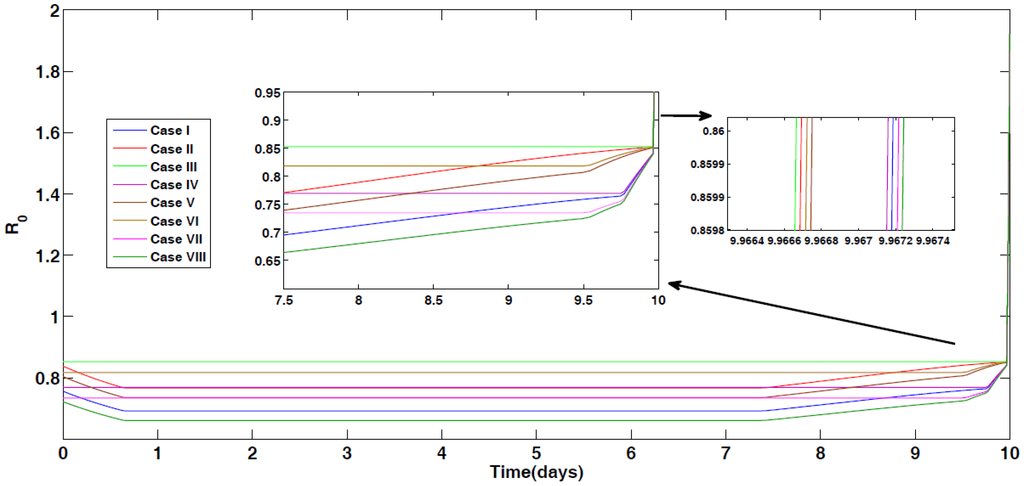
4.1. Optimal Control for Different Cases

We applied all the controls continuously. We used a combination of controls for prevention of the disease, and compared all the scenarios. Actually, we compared the cases when one, two, three, and all the controls are applied separately. In fact, we do not know which combination is better to obtain the desired cost-effective result. We numerically constructed Figure A1, Figure A2, Figure A3, Figure A4, Figure A5, Figure A6, Figure A7 and Figure A8, indicating when a particular case is better than the others. Thus, we have consider all the cases for examination.

We numerically investigated the effect of the following optimal controls on the spread of leishmaniasis in a population for different cases [33,34].

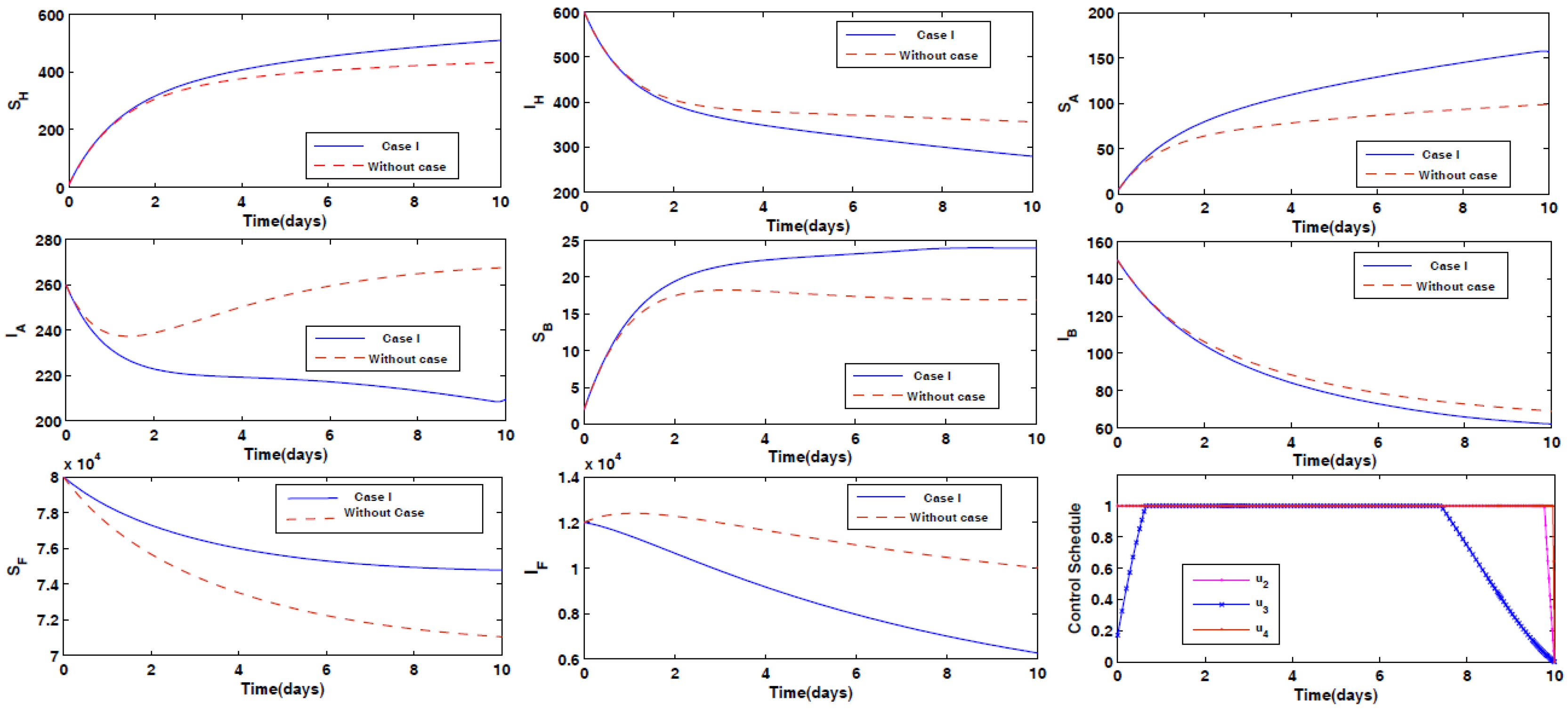
• Case I: Prevention of the infection of animals Type A and Type B by the disease, along with spraying insecticides on the sand fly vectors.
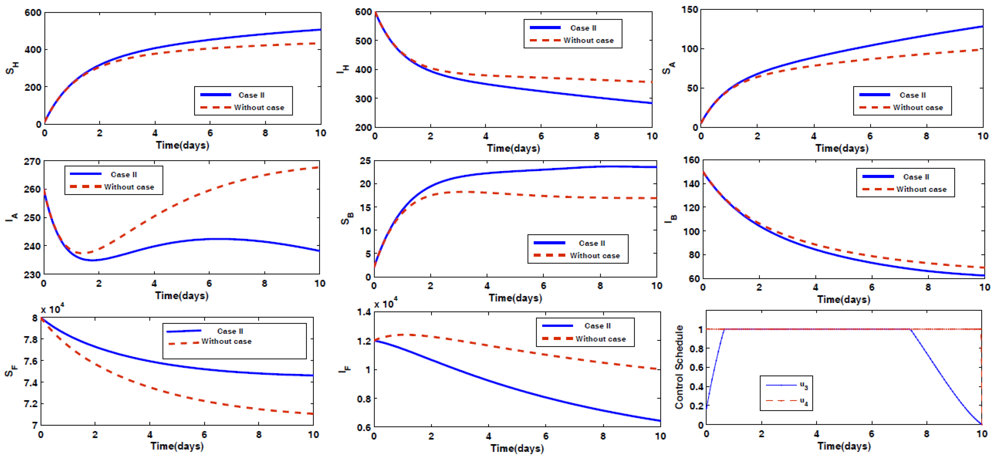
• Case II: Prevention of animal Type B being infected by the disease, along with spraying insecticides on the sand fly vectors.
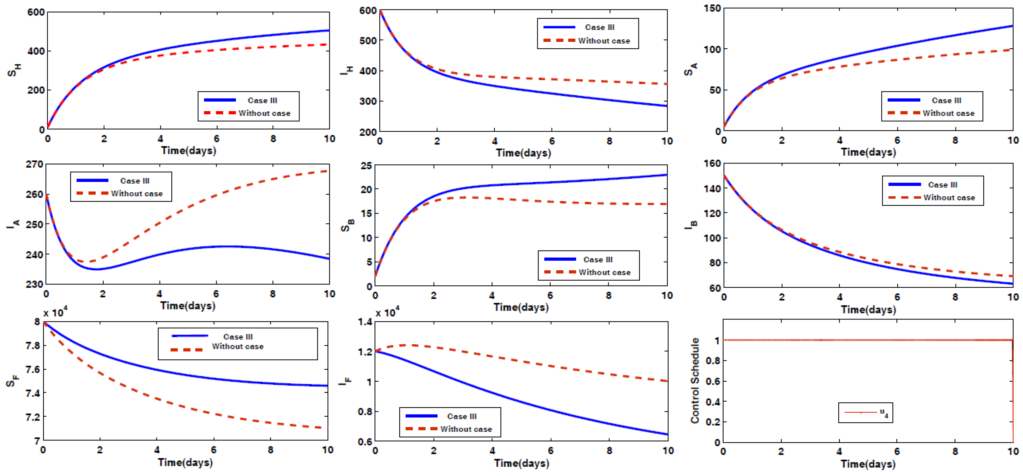
• Case III: Spraying insecticides on the sand fly vectors.
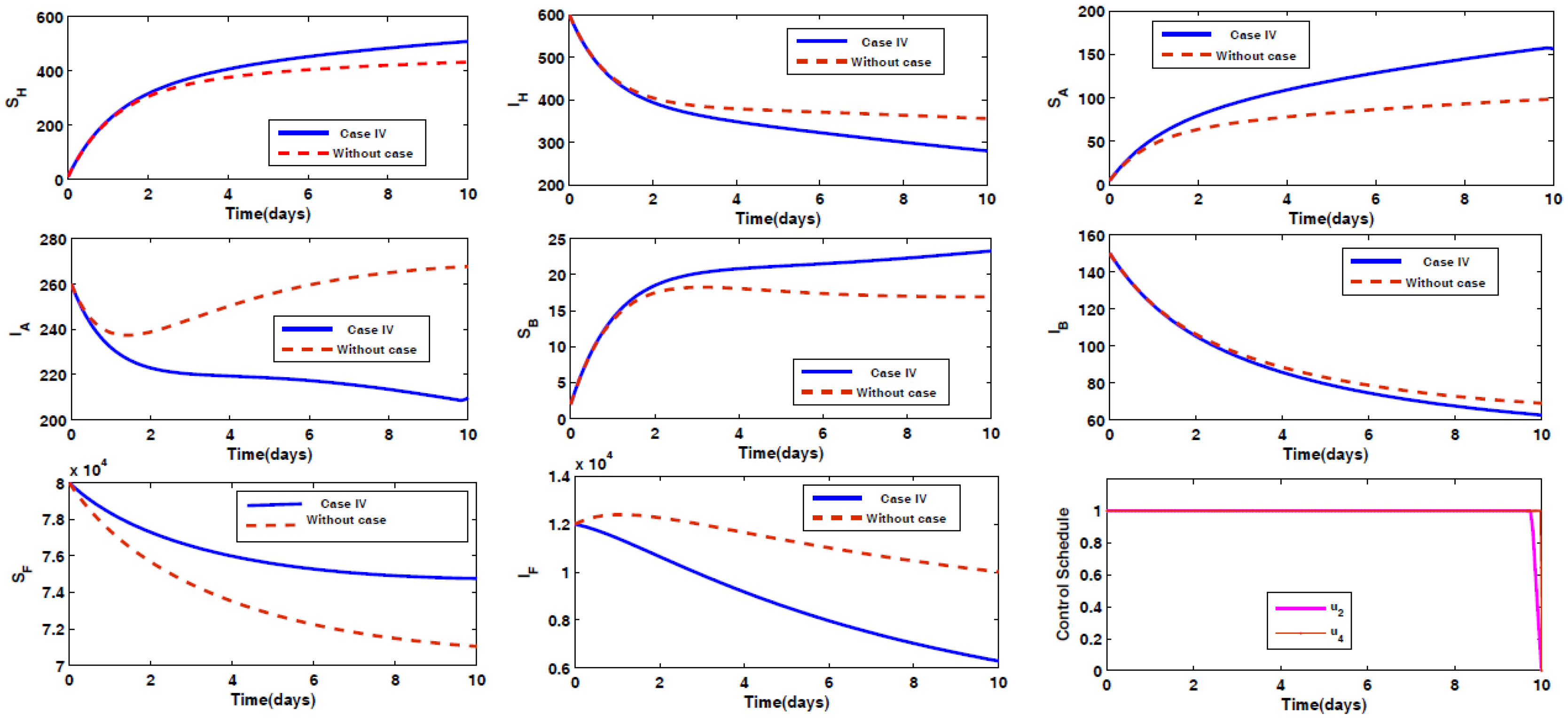
• Case IV: Prevention of animal Type A being infected by the disease, along with spraying insecticides on the sand fly vectors.
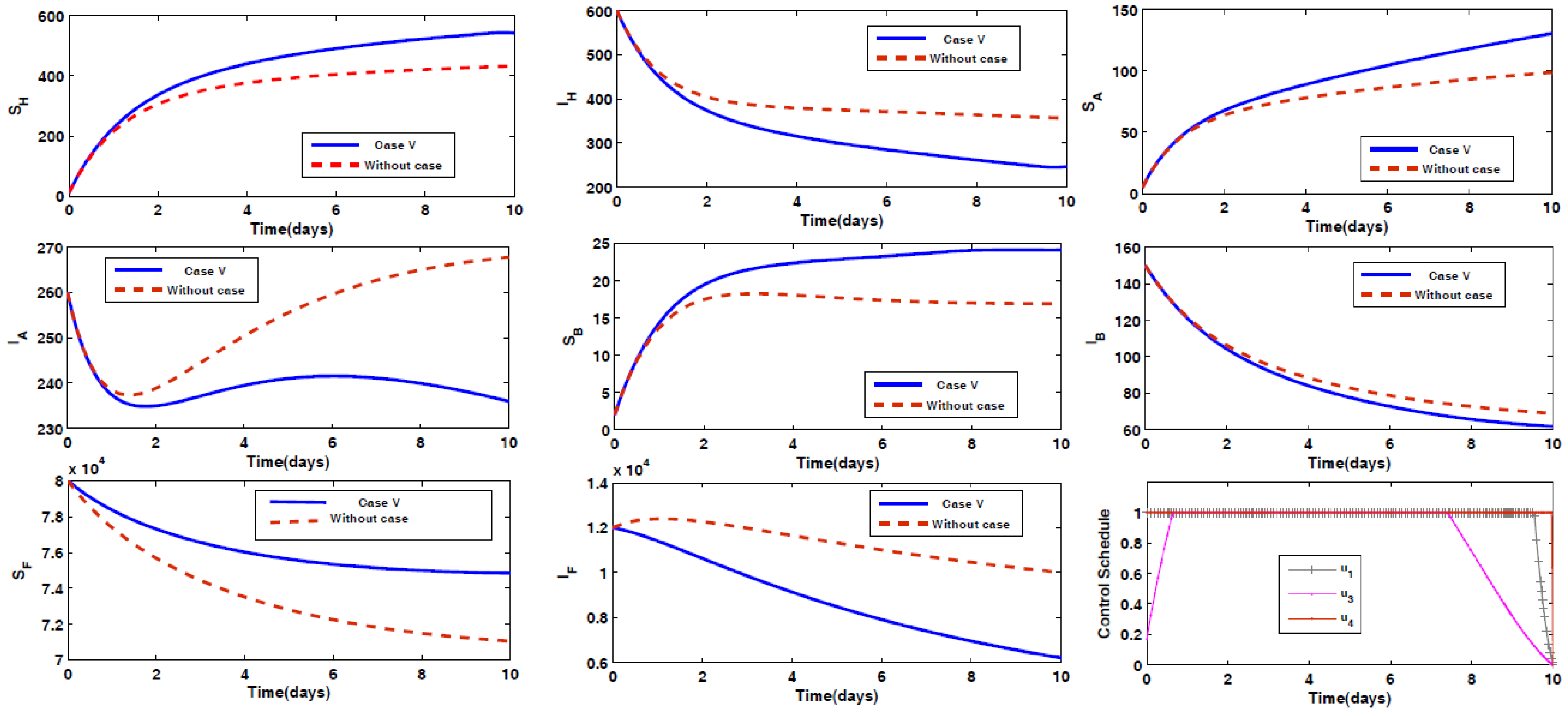
• Case V: Prevention of animal Type B being infected by the disease, along with spraying insecticides on the sand fly vectors.
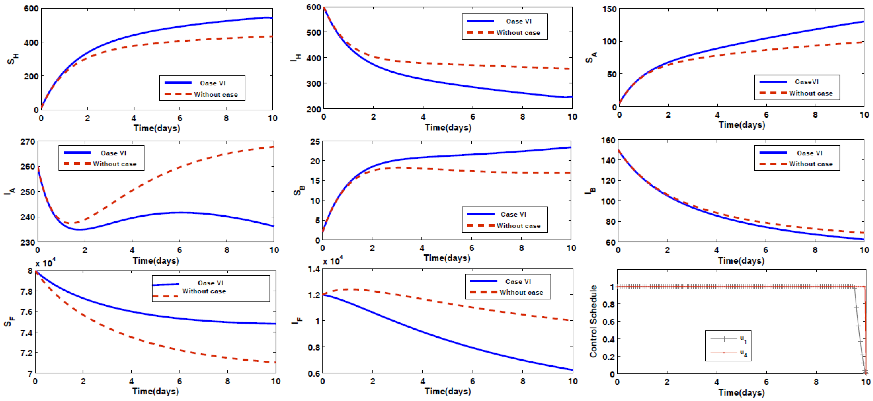
• Case VI: Prevention of humans being infected by the disease, along with spraying insecticides on the sand fly vectors.
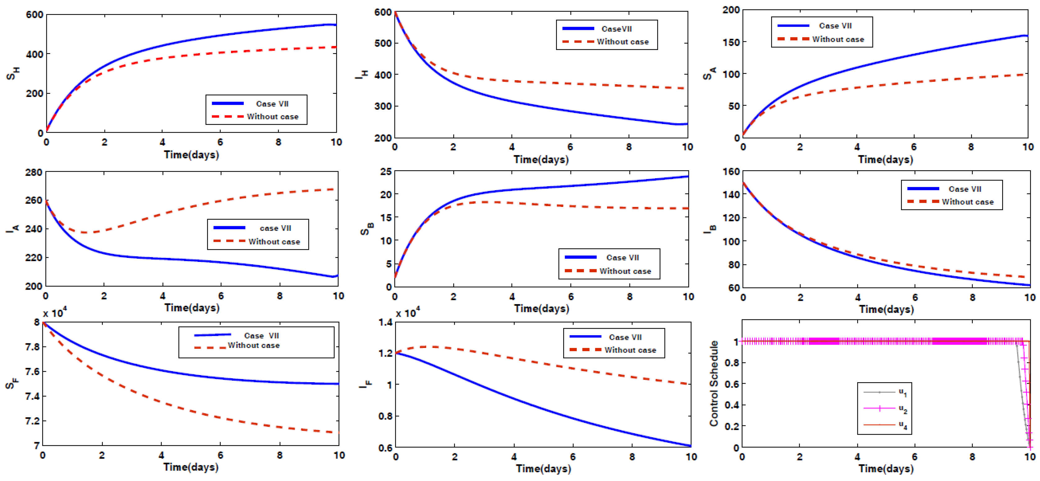
• Case VII: Prevention of humans and animal Type A being infected by the disease, along with spraying insecticides on the sand fly vectors.
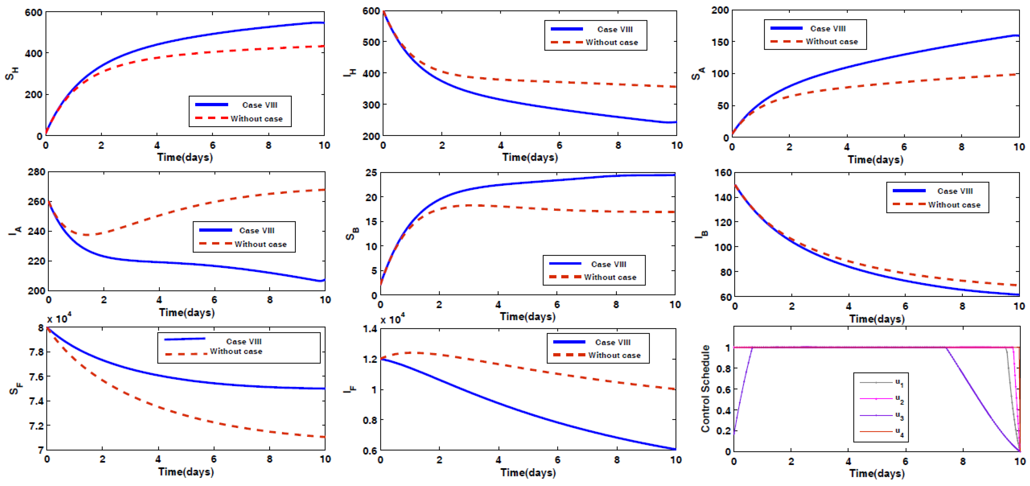
• Case VIII: Prevention of humans and animals Type A and Type B being infected by the disease, along with spraying insecticides on the sand fly vectors.

See Appendix A.

4.2. Impact of Optimal Control on the Different Cases Proposed

We aimed to describe the long-term behavior of the disease prevalence for the future, which cannot be predicted by the application of the optimal control strategies used in our model. After effective strategies are stopped, there are often some infectious people remaining who can cause a fresh outbreak of the disease [35]. Since the basic reproduction number proved to be effective in measuring long-term endemicity in [23], the effects of our applied strategies on $\left(R_0\right)$ were studied. Figure 7 demonstrates the results of numerical simulation of $\left(R_0\right)$ under the various control strategy approaches. Assuming that the combinations of optimal control were implemented in the beginning of the year, it was observed that case VIII performed well in the early stages, and also kept the disease under check. Cases I, VII, V, IV, II, VI, and III performed almost similarly throughout.

For longer time periods, $R_0$ increased, at which point further application of control policies becomes necessary. Thus, the implementation of different strategies during different points of time produces different disease dynamics. Hence, it becomes important to determine the exact point in time at which the effective strategy needs to be implemented. Further, the complete elimination of the disease by effective application of the control strategy can be possible only if these strategies are continued over long time periods, by determination of the class boundaries of the controls $u_1$, $u_2$, $u_3$, and $u_4$.

Figure S3 describes the numerical simulation outcomes of $R_0$ for the various cases of control strategies applied to each population.

4.3. Rescued Population and Vector Reduction for Different Cases

The useful data for finding rescued population-based strategy are in

Table 2. Reduction in infected host population (%).

Cases	Human	Animal A	Animal B	Vector Reduction
Case I	12.67	22.31	4.67	31.10
Case II	12	11.15	4.67	29.7
Case III	11.83	11.15	4.00	29.54
Case IV	12.50	12.92	4.00	30.90
Case V	18.16	5.17	4.67	31.54
Case VI	18	11.92	4.67	31.38
Case VII	18.5	23.07	4.67	32.75
Case VIII	18.60	23.07	5.33	32.92

. The maximum number of humans were rescued within time in Cases VIII and VII, and the minimum number of humans were rescued in Cases III and II. The maximum number of infected animals of Type A were extricated within time in Cases VII and VIII, and the minimum number of animals of Type A were extricated in Case V. The maximum number of animals of Type B were rescued within time in Case VIII, and the minimum number of animals of Type B were rescued in Cases III and IV. The maximum vector reduction occurred within time in Cases VIII and VII, followed by Case II, and the minimum reduction occurred in Case III. Therefore, we can say empirically that the maximum number of humans were rescued in time when implementing Case VIII. Additionally, the maximum number of vectors were reduced in time compared to the other strategies. However, this cannot be the most cost-effective approach because of all of the drugs and insecticides which are applied to each of the populations to control the disease.

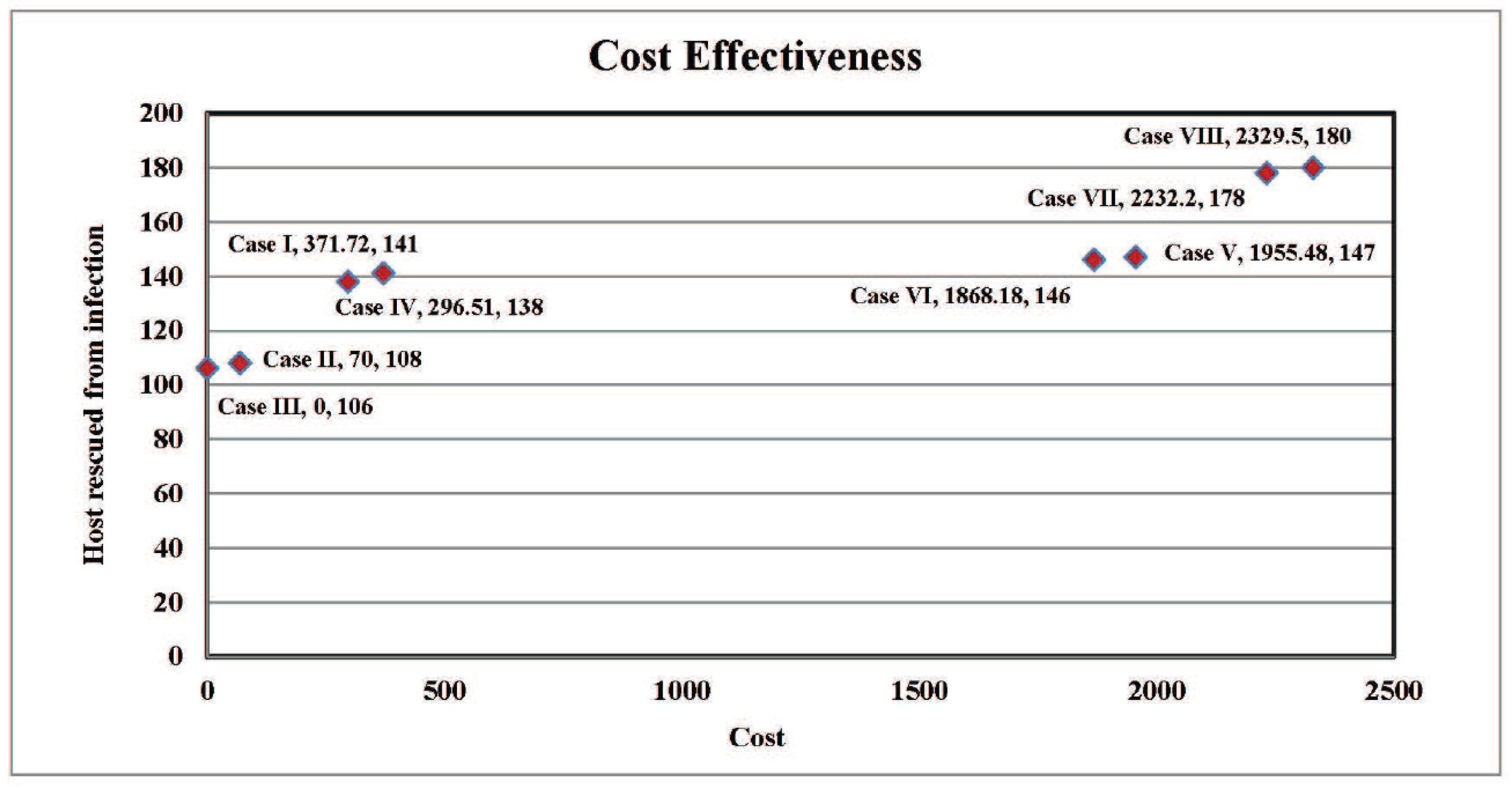
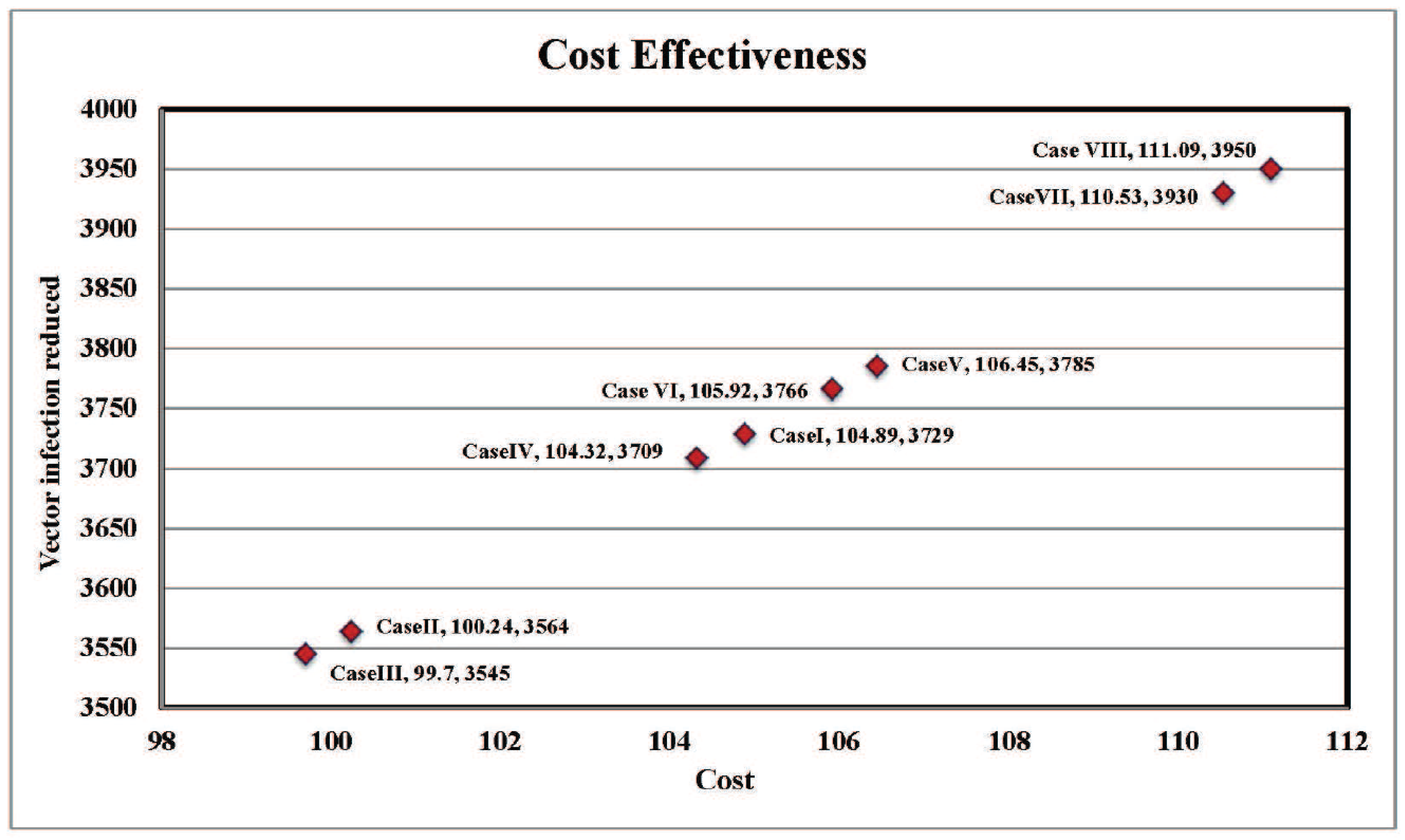
4.4. Cost-Effectiveness of the Different Cases

Herein, we consider the size of the population rescued from infection as well as the extent of vector reduction with the different control strategies. For this, we assumed that the cost of the controls were the square of the proportional to the number of controls deployed, and considered the cost of drug $u_1$ per person to be approximately 1.86$ (in INR 118.94) [36], the cost of drug $u_2$ per Type A animal to be 1.2$ (in INR 76.74), the cost of drug $u_3$ per Type B animal to be 1$ (in INR 63.95), and the cost of insecticide spraying $u_4$ per square meter area for vector death to be 1.5$ (in INR 95.92). The assumption was based on the understanding that the primary goal of using the drug is for the cure of those infected by the disease. Moreover, the use of insecticides is for the removal of vector. The difference between the total size of the infectious population without control and with control was used to determine the number of infections averted. We used the size of the rescued population and extent of vector reduction, as depicted in

Table 3. Cost-effectiveness for different cases.

Cases	Host Reduction	Cost (in $)	Vector Reduced	Cost (in $)
Case I	141	371.716	3729	104.878
Case II	108	70	3564	100.238
Case III	106	0	3545	99.70
Case IV	138	296.514	3709	104.316
Case V	147	1955.482	3785	106.453
Case VI	146	1868.184	3766	105.919
Case VII	178	2232.198	3930	110.531
Case VIII	180	2329.496	3950	111.094

. The control strategy applied in the model gave maximum cost benefit. This was determined for each intervention strategy, illustrated in Figure 8 and Figure 9. One can see that the most cost-effective cases in terms of number of infections averted, including the number reduction of the sand fly vector, was the spraying of insecticides (Case III).

4.5. Discussion

The disease leishmaniasis spreads from animal (reservoir) to human (host) via a vector. For this reason, the control of vectors and infected reservoir populations is one of the most efficient approaches to exterminating the disease cutaneous leishmaniasis. Applying a suitable drug to the reservoir population and spraying insecticide to kill the vector perform significant functions for controlling CL. We investigated the dynamics in the absence of drug applied in human hosts and animals, and without the spraying of insecticide to kill the vector. The disease-free situation existed for $R_0<1$. On the other hand, if $R_0>1$, the disease-free state lost its stability and the system tended towards the endemic condition.

From Figure 5, we observe that susceptible human host population was sharply decreased up to approximately 30 days, and the infected human host population gradually increased up to approximately 30 days. Susceptible animal of Type A sharply decreased up to approximately 25 days and susceptible animal of Type B sharply decreased up to approximately 20 days. Again, the infected animal population of Type A gradually increased up to approximately 25 days, and the population of infected animals of Type B gradually increased up to approximately 20 days. The susceptible sand fly population increased up to approximately 12 days, and the infected sand fly population gradually increased up to approximately 20 days. Thus, we can conclude that the disease can be controlled by insecticide spraying with a frequency appropriate to the size of the vector population. The change of the behavioral structure of the system dynamics depends on the biting rate and the transmission possibility of the sand fly. So, if we are able to kill the sand fly by spraying insecticide, then biting rate and transmission will automatically be reduced and then the disease can be controlled.

The inclusion of latent and recovered categories and the use of delayed terms in the model equation system may change the dynamics of the disease. However, the life cycle of the parasite is not long enough to support the incubation period. Therefore, we did not consider the latent status in our model. Additionally, the progression from susceptible to infected classes passes through a latent stage. So, we ignored the intermediate stages (latent and recovered) and considered susceptible and infected stages only. We paid no attention to the delay term, because our main aim was to control the infected population and the vector. Consequently, we considered the delay term to be in steady state.

The effectiveness of the drug dose influences the system to move towards the infection-free state. The results obtained from analytical and numerical simulations showed that the control strategies were very effective if applied at the same time in the same region. The proposed optimal control can eradicate and prevent further transmission of the disease through the vector. Although total eradication of cutaneous leishmaniasis seems complicated in a realistic environment, if our findings can be applied to an infected zone, then a pioneering insight can be achieved against cutaneous leishmaniasis in a global perspective.

To prevent vector-borne disease, different strategic cases can be applied to a finite time period. The effects of the different cases used to minimize the disease among the various populations were investigated using the analysis of optimal control, thereby depicting the real situations. Herein, we considered four controls upon three types of mammalian host and a vector population: prevention of infective individuals by using drugs and spraying of insecticides to kill vector. It was deduced that the strategy applied in Case I yielded good results for a considerable time period, however Case III was most cost effective but did not achieve as great a reduction in infected host or vector in the same time period. For the entire period of the preventive measure, the effects of our control strategies on $R_0$ were observed to determine the effects of the controls on the future spread of disease. The significant changes in the number of possible secondary infections from an infected individual were thus concluded to be dependent on time. Thus, it becomes important to determine the exact time interval during which the optimal control must be applied. Moreover, it is only possible to eliminate the disease entirely if the different control strategies are continued for a long duration in the future.

5. Conclusions

From the study of the effects of the various control cases on $R_0$, it was observed that Case VIII yielded the best results in attempting to control the disease, followed by Cases VII and V. The analysis of cost-effectiveness indicated that Case III was the most cost-effective, followed by Case II. Though the potential of Case I in trying to eliminate the disease is comparatively better than that of Case IV, it involves higher costs. It can be concluded that the cases which display low disease prevalence would require an efficient and cost-effective strategy (Cases II and IV). However, the cases where the utmost priority is to control the disease would require strategic cases that are less cost-effective but act efficiently to control the disease in a short time period (e.g., Case I). Hence, our model would suffice in assisting decisions related to the allocation of resources, where the fundamental aim is to select the best strategy to eliminate the disease in the lowest possible time.

References

1. Sharma, U.; Singh, S. Immunobiology of leishmaniasis. Indian J. Exp. Biol. 2009, 47, 412–423. [Google Scholar] [PubMed]
2. Park, K. Preventive and Social Medicine; Banarsidas Bhanot Publishers: Jabalpur, India, 2005. [Google Scholar]
3. Chaves, L.F.; Hernandez, M.J. Mathematical modelling of American Cutaneous Leishmaniasis: Incidental hosts and threshold conditions for infection persistence. Acta Trop. 2004, 92, 245–252. [Google Scholar] [CrossRef] [PubMed]
4. World Health Organization. Leishmaniasis. Fact Sheet Updated April 2017. Available online: http://www.who.int/news-room/fact-sheets/detail/leishmaniasis (accessed on 18 July 2018).
5. ELmojtaba, I.M.; Mugisha, J.Y.T.; Hashim, M.H.A. Mathematical analysis of the dynamics of visceral leishmaniasis in the Sudan. Appl. Math. Comput. 2010, 217, 2567–2578. [Google Scholar] [CrossRef]
6. Kassiri, H.; Sharifinia, N.; Jalilian, M.; Shemshad, K. Epidemiological aspects of cutaneous leishmaniasis in Ilam province, west of Iran (2000–2007). Asian Pac. J. Trop. Dis. 2012, 2, S382–S386. [Google Scholar] [CrossRef]
7. Reithinger, R.; Dujardin, J.C.; Louzir, H.; Pirmez, C.; Alexander, B.; Brooker, S. Cutaneous leishmaniasis. Lancet Infect. Dis. 2007, 7, 581–596. [Google Scholar] [CrossRef]
8. Kasper, D.L.; Braunwald, E.; Fauci, A.S.; Hauser, S.L.; Longo, D.L.; Jameson, J.L.; Loscalzo, J. Harrison’s Principles of Internal Medicine, 17th ed.; McGraw-Hill: New York, NY, USA, 2008; Volume 1, Chapter 1–216. [Google Scholar]
9. Bathena, K. A Mathematical Model of Cutaneous Leishmaniasis. Master’s Thesis, Rochester Institute of Technology, Rochester, NY, USA, 2009. [Google Scholar]
10. Miller, E.; Huppert, A. The effects of Host Diversity on Vector-Borne Disease: The Conditions under Which Diversity Will Amplify or Dilute the Disease Risk. PLoS ONE 2013, 8, e80279. [Google Scholar] [CrossRef] [PubMed]
11. Jaouadi, K.; Haouas, N.; Chaara, D.; Gorcii, M.; Chargui, N.; Augot, D.; Pratlong, F.; Dedet, J.P.; Ettlijani, S.; Mezhoud, H.; et al. First detection of Leishmania killicki (Kinetoplastida, Trypanosomatidae) in Ctenodactylus gundi (Rodentia, Ctenodactylidae), a possible reservoir of human cutaneous leishmaniasis in Tunisia. Parasites Vectors 2011, 4, 159. [Google Scholar] [CrossRef] [PubMed] [Green Version]
12. Chatterjee, A.N.; Roy, P.K.; Mondal, J. Mathematical Model for Suppression of Sand Flies through IRS with DDT in Visceral Leishmaniasis. Am. J. Math. Sci. 2013, 2, 105–112. [Google Scholar]
13. Wu, H.J.J.; Massad, E. Mathematical modelling for Zoonotic Visceral Leishmaniasis dynamics: A new analysis considering updated parameters and notified human Brazilian data. Infect. Dis. Model. 2017, 2, 143–160. [Google Scholar]
14. Bacaer, N.; Guernaoui, S. The epidemic threshold of vector-borne diseases with seasonality the case of cutaneous leishmaniasis in Chichaoua, Morocco. J. Math. Biol. 2006, 53, 421–436. [Google Scholar] [CrossRef] [PubMed]
15. Biswas, D.; Kesh, D.K.; Datta, A.; Chatterjee, A.N.; Roy, P.K. A Mathematical Approach to Control Cutaneous Leishmaniasis Through Insecticide Spraying. Sop Trans. Appl. Math. 2014, 1, 44–54. [Google Scholar] [CrossRef]
16. Biswas, D.; Roy, P.K.; Li, X.Z.; Basir, F.A.; Pal, J. Role of macrophage in the disease dynamics of cutaneous leishmaniasis: A delay induced mathematical study. Commun. Math. Biol. Neurosci. 2016, 2016, 1–31. [Google Scholar]
17. Roy, P.K.; Li, X.Z.; Biswas, D.; Datta, A. Impulsive Application to Design Effective Therapies Against Cutaneous Leishmaniasis Under Mathematical Perceptive. Commun. Math. Biol. Neurosci. 2017, 2017, 1–17. [Google Scholar]
18. Biswas, D.; Datta, A.; Roy, P.K. Combating Leishmaniasis through Awareness Campaigning: A Mathematical Study on Media Efficiency. Int. J. Math. Eng. Manag. Sci. 2016, 1, 139–149. [Google Scholar]
19. Zamir, M.; Zaman, G.; Alshomrani, A.S. Sensitivity Analysis and Optimal Control of Anthroponotic Cutaneous Leishmania. PLoS ONE 2016, 11, e0160513. [Google Scholar] [CrossRef] [PubMed]
20. Begon, M.; Bennett, M.; Bowers, R.G.; French, N.P.; Hazel, S.M.; Turner, J. A clarication of transmission terms in host-microparasite models: numbers, densities and areas. Epidemiol. Infect. 2002, 129, 147–153. [Google Scholar] [CrossRef] [PubMed]
21. Abubakar, A.; Ruiz-Postigo, A.J.; Pita, J.; Lado, M.; Ben-Ismail, R.; Argaw, D.; Alvar, J. Visceral leishmaniasis outbreak in South Sudan 2009–2012: Epidemiological assessment and impact of a multisectoral response. PLoS Negl. Trop Dis. 2014, 8, e2720. [Google Scholar] [CrossRef] [PubMed]
22. Subramanian, A.; Singh, V.; Sarkar, R.R. Understanding Visceral Leishmaniasis Disease Transmission and its Control—A Study Based on Mathematical Modeling. Mathematics 2015, 3, 913–944. [Google Scholar] [CrossRef] [Green Version]
23. Biswas, S.; Subramanian, A.; ELMojtaba, I.M.; Chattopadhyay, J.; Sarkar, R.R. Optimal combinations of control strategies and cost-effective analysis for visceral leishmaniasis disease transmission. PLoS ONE 2017, 12, e0172465. [Google Scholar] [CrossRef] [PubMed]
24. Brett-Major, D.M.; Claborn, D.M. sandfly Fever: What Have We Learned in One Hundred Years? Mil. Med. 2009, 174, 426–431. [Google Scholar] [CrossRef] [PubMed]
25. Rogers, M.E.; Bates, P.A. Leishmania Manipulation of sandfly Feeding Behavior Results in Enhanced Transmission. PLoS Pathog. 2007, 3, e91. [Google Scholar] [CrossRef] [PubMed] [Green Version]
26. Lopez, L.F.; Coutinho, F.A.B.; Burattini, M.N.; Massad, E. Threshold conditions for infection persistence in complex host-vectors interactions. Comptes Rendus Biol. 2002, 325, 1073–1084. [Google Scholar] [CrossRef]
27. Zaman, G.; Kang, Y.H.; Jung, I.H. Stability analysis and optimal vaccination of an SIR epidemic model. BioSystems 2008, 93, 240–249. [Google Scholar] [CrossRef] [PubMed]
28. Birkhoff, G.; Rota, G.C. Ordinary Differential Equations, 4th ed.; John Wiley and Sons: New York, NY, USA, 1989. [Google Scholar]
29. Lukes, D.L. Differential Equations: Classical to Controlled in Mathematics in Science and Engineering; Academic Press: New York, NY, USA, 1982; Volume 162. [Google Scholar]
30. Kirschner, D.; Lenhart, S.; Serbin, S. Optimal control of the chemotherapy of HIV. J. Math. Biol. 1997, 35, 775–792. [Google Scholar] [CrossRef] [PubMed] [Green Version]
31. Shimozako, H.J.; Wu, J.; Massad, E. The Preventive Control of Zoonotic Visceral Leishmaniasis: Efficacy and Economic Evaluation. Comput. Math. Methods Med. 2017, 2017, 4797051. [Google Scholar] [CrossRef] [PubMed]
32. Kaabi, B.; Ahmed, S.B. Assessing the effect of zooprophylaxis on zoonotic cutaneous leishmaniasis transmission: A system dynamics approach. Biosystems 2013, 114, 253–260. [Google Scholar] [CrossRef] [PubMed]
33. Okosuna, K.O.; Rachid, O.; Marcus, N. Optimal control strategies and cost-effectiveness analysis of a malaria model. BioSystems 2013, 111, 83–101. [Google Scholar] [CrossRef] [PubMed]
34. Sardar, T.; Mukhopadhyay, S.; Bhowmick, A.R.; Chattopadhyay, J. An optimal cost effectiveness study on Zimbabwe cholera seasonal data from 2008–2011. PLoS ONE 2013, 8, e81231. [Google Scholar] [CrossRef] [PubMed]
35. Stauch, A.; Sarkar, R.R.; Picado, A.; Ostyn, B.; Sundar, S.; Rijal, S.; Boelaert, M.; Dujardin, J.; Duerr, H. Visceral Leishmaniasis in the Indian Subcontinent: Modelling Epidemiology and Control. PLoS Negl. Trop. Dis. 2011, 5, e1405. [Google Scholar] [CrossRef] [PubMed]
36. Costs of Medicines in Current Use for the Treatment of Leishmaniasis (Annex6), Drug Prices (January 2010). Available online: http://www.who.int/leishmaniasis/research/978_92_4_12_949_6_Annex6.pdf (accessed on 18 July 2018).
Figure 1. Schematic diagram of the model system (1) with flow of transmission.
Mca 23 00038 g001
Figure 2. Cumulative number of leishmaniasis cases for the period January–December 2012. CL: cutaneous leishmaniasis.
Mca 23 00038 g002
Figure 3. Panel A shows cumulative new leishmaniasis cases for the period January–December 2013 from data, and Panel B shows the model simulated data plotted using estimated parameter values. Panel C shows that the simulated parametric data values coincided with real data values, thus validating the model.
Mca 23 00038 g003
Figure 4. Population densities of the model variables for R 0 < 1 for disease-free state (all parameters are in Table 1).
Mca 23 00038 g004
Figure 5. Population densities of the model variables for R 0 > 1 (other parameters are as in Table 1).
Mca 23 00038 g005
Figure 6. Behavior of the model system with optimal control schedule of the drug therapy.
Mca 23 00038 g006
Figure 7. Effect of different control cases on R 0 and magnified for t = 7.5–10 days.
Mca 23 00038 g007
Figure 8. Cost of different cases and their corresponding rescued host population plotted as a scatter diagram.
Mca 23 00038 g008
Figure 9. Cost of different cases and their corresponding vector infection reduced plotted as a scatter diagram.
Mca 23 00038 g009