A Complex Variable Solution for Lining Stress and Deformation in a Non-Circular Deep Tunnel II Practical Application and Verification

Abstract

A new complex variable method is presented for stress and displacement problems in a non-circular deep tunnel with certain given boundary conditions at infinity. In order to overcome the complex problems caused by non-circular geometric configurations and the multiply-connected region, a complex variable method and continuity boundary conditions are used to determine stress and displacement within the tunnel lining and within the surrounding rock. The coefficients in the conformal mapping function and stress functions are determined by the optimal design and complex variable method, respectively. The new method is validated by FLAC3D finite difference software through an example. Both the new method and the numerical simulation obtained similar results for the stress concentration and the minimum radial displacement occurred at a similar place in the tunnel. It is demonstrated that the new complex variable method is reliable and reasonable. The new method also provides another way to solve non-circular tunnel excavation problems in a faster and more accurate way.

1. Introduction

With the rapid economic development in China, which has caused the expansion of road and railway networks from east to west and to areas in the northeast that are surrounded by mountains, the construction of tunnels is broadly used to improve existing transportation networks. Lining is the primary support adopted to ensure rock pressure. It has been of high interest in determining stress fields within lining using analytical methods. Analytical solutions for stress distribution within circular lining and around circular and elliptical holes have been proposed by many authors (Bobet [1,2]; Lee and Nam [3]; Timoshenko and Goodier [4]).

Many studies have been carried out to determine the stress and deformation of tunnels by applying numerical methods, which have been generally used to provide an understanding of how the stress and deformation of lining are influenced by different parameters. Numerical methods are largely employed to find the stress and deformation stages of lining in the preliminary stages of design.

Muskhelishvili’s [5] complex variable method is one of the useful analytical approaches that fully expounded a basic theory of complex potential functions in order to address some issues of plane elasticity mechanics. Based on this method, Exadaktyol and Stavtopoulou [6,7] proposed a closed-form plane strain solution for stress and displacement around semicircular holes. Verruijt [8,9] calculated the stress and displacement components around a circular tunnel in an elastic half-plane. Zhao and Yang [10] obtained a general solution for deep square tunnels with different pressure coefficients. Kargar et al. [11] made an attempt to study lining stress and deformation in a non-circular deep tunnel using the Cauchy integral formula of complex variable methods. Li and Chen [12] obtained analytical solutions for a non-circular tunnel lining in power series forms. However, the analytical solutions for stress and displacement found in the above-mentioned literature have seldom come to an available expression for non-circular deep tunnels, especially non-circular deep tunnels with a lining, except for Kargar et al. [11] and Li [12].

When considering the problem with circular support, the solution is much easier. When a non-circular lining is included, the problem considers a multiply-connected region and conformal mapping, which increases the complexity of the problem. Kargar’s [11] method can calculate the stress of a non-circular deep tunnel with a lining, although the method needs to integrate. The integral is too complex and difficult to calculate. Li’s [12] method only considered the non-circular tunnel lining without thinking about the surrounding rock around the lining. In order to simplify the calculation, Li [12] assumed that the surrounding rock has a certain given surface traction applied to the lining. In this study it will be shown that these difficulties can be surmounted at last for the case of a non-circular deep tunnel with certain boundary conditions at infinity, by a new complex variable method in power series forms.

Based on the research findings proposed, an attempt was made in this paper to find the stress distribution and radial displacement of the lining in a non-circular deep tunnel, considering the boundary conditions of the surrounding rocks by applying a complex variable power series method, which is more efficient, simple and accurate. Finally, the new method was validated by the FLAC finite difference software through an example.

2. Problem Statement and General Consideration

The problem refers to a non-circular tunnel with lining in an elastic geomaterial. The tunnel is located at great depth compared with the tunnel dimension; the problem is considered a single hole with support in an infinite plane. The infinite plate on the complex plane is divided into the two isotropic homogenous regions of S₁ and S₂ bounded by contours L₁ and L₂. The regions S₁ and S₂ refer to the lining and the surrounding rock, respectively. The boundary of the tunnel lining inside (L₁) is free of stress, and the rock-lining interface (L₂) satisfies the continuity boundary conditions. It is assumed that the region S₁ in the z-plane can be mapped conformally onto a ring (O₁) in the $\mathsf{\zeta }$-plane. The surrounding rock, region S₂ in the z-plane, can be mapped conformally onto the region O₂, which is the area outside the L₂ outline in the $\mathsf{\zeta }$-plane, see Figure 1. The general formula of the conformal mapping function is determined based on the Laurent series as follows:

$$\mathrm{w}(\mathsf{\zeta })=\mathrm{R}(\mathsf{\zeta }+{\displaystyle \sum }_{\mathrm{k}=0}^{\infty }{\mathrm{J}}_{\mathrm{k}}{\mathsf{\zeta }}^{-\mathrm{k}})$$

(1)

where R is positive real number reflecting the hole’s size, and the ${\mathrm{J}}_{\mathrm{k}}$ are generally complex numbers, which are determined by the shape of the tunnel. In most situations it is accurate enough to only take the first few of ${\mathrm{J}}_{\mathrm{k}}$ of the series. $\mathsf{\theta }$ and $\mathsf{\rho }$ are assumed to be two polar coordinates of point $\mathsf{\zeta }$ in the $\mathsf{\zeta }$-plane.

In the complex variable method [5,13,14], the solution is expressed in terms of two functions $\mathsf{\phi }$ and $\mathsf{\psi }$, which must be analyzed in the region S₁ occupied by the elastic material. The stresses are determined based on the stress functions in the equations:

$${\mathsf{\sigma }}_{\mathsf{\theta }}+{\mathsf{\sigma }}_{\mathsf{\rho }}=4\mathrm{Re}\left[\frac{{\mathsf{\phi }}^{\prime }(\mathsf{\zeta })}{{\mathrm{w}}^{\prime }(\mathsf{\zeta })}\right]$$

(2)

$${\mathsf{\sigma }}_{\mathsf{\theta }}-{\mathsf{\sigma }}_{\mathsf{\rho }}+{\mathsf{\tau }}_{\mathsf{\rho }\mathsf{\theta }}=\frac{2{\mathsf{\zeta }}^2}{{\mathsf{\rho }}^2}\frac{1}{\overline{{\mathrm{w}}^{\prime }(\mathsf{\zeta })}}\left[\overline{\mathrm{w}(\mathsf{\zeta })}\frac{{\mathsf{\phi }}^{″}(\mathsf{\zeta }){\mathrm{w}}^{\prime }(\mathsf{\zeta })-{\mathsf{\phi }}^{\prime }(\mathsf{\zeta }){\mathrm{w}}^{″}(\mathsf{\zeta })}{{\mathrm{w}}^{\prime }(\mathsf{\zeta }){\mathrm{w}}^{\prime }(\mathsf{\zeta })}+{\mathsf{\psi }}^{\prime }(\mathsf{\zeta })\right]$$

(3)

where ${\mathsf{\sigma }}_{\mathsf{\rho }}$, ${\mathsf{\sigma }}_{\mathsf{\theta }}$ and ${\mathsf{\tau }}_{\mathsf{\rho }\mathsf{\theta }}$ are the radial, circumferential and tangential stress components, respectively.

The displacements are given by

$$2\mathrm{G}({\mathrm{u}}_{\mathsf{\rho }}+{\mathrm{iu}}_{\mathsf{\theta }})=\frac{\overline{\mathsf{\zeta }}}{\mathsf{\rho }}\frac{\overline{{\mathrm{w}}^{\prime }(\mathsf{\zeta })}}{\left|\mathrm{w}(\mathsf{\zeta })\right|}\left[\mathsf{\kappa }\mathsf{\phi }(\mathsf{\zeta })-\frac{\mathrm{w}(\mathsf{\zeta })}{\overline{{\mathrm{w}}^{\prime (\mathsf{\zeta })}}}\overline{{\mathsf{\phi }}^{\prime }(\mathsf{\zeta })}-\overline{\mathsf{\psi }(\mathsf{\zeta })}\right]$$

(4)

where G is the shear modulus of the elastic material, and $\mathsf{\kappa }$ is determined by Poisson’s ratio $\mathsf{\upsilon }$, $\mathsf{\kappa }=3-4\mathsf{\upsilon }$ and $\mathsf{\kappa }=\frac{3-\mathsf{\upsilon }}{1+\mathsf{\upsilon }}$ are plane strain and plane stress, respectively. In this paper, plane strain conditions are assumed. Based on the Kargar’s [11] method and Chen [15], the stress functions ${\mathsf{\phi }}_1$ and ${\mathsf{\psi }}_1$ in the region O₂ have the following expansions:

$${\mathsf{\phi }}_1(\mathsf{\zeta })=\Gamma \mathrm{w}(\mathsf{\zeta })+{\mathsf{\phi }}_0(\mathsf{\zeta })$$

(5)

$${\mathsf{\psi }}_1(\mathsf{\zeta })={\Gamma }^{\prime }\mathrm{w}(\mathsf{\zeta })+{\mathsf{\psi }}_0(\mathsf{\zeta })$$

(6)

where

$${\mathsf{\phi }}_0(\mathsf{\zeta })={\displaystyle \sum }_{\mathrm{k}=0}^{\infty }{\mathrm{h}}_{\mathrm{k}}{\mathsf{\zeta }}^{-\mathrm{k}}$$

(7)

$${\mathsf{\psi }}_0(\mathsf{\zeta })={\displaystyle \sum }_{\mathrm{k}=0}^{\infty }{\mathrm{m}}_{\mathrm{k}}{\mathsf{\zeta }}^{-\mathrm{k}}$$

(8)

where ${\mathrm{h}}_{\mathrm{k}}$, ${\mathrm{m}}_{\mathrm{k}}$ are generally complex numbers, which must be determined from boundary conditions.

${\mathsf{\phi }}_0(\mathsf{\zeta })$ and ${\mathsf{\psi }}_0(\mathsf{\zeta })$ are holomorphic functions with ${\mathsf{\phi }}_0(\infty )=0$ and ${\mathsf{\psi }}_0(\infty )=0$, $\Gamma$ and ${\Gamma }^{\prime }$ are real and complex constants with regard to the stress state at infinity, which are determined as follows:

$$\Gamma =\frac{1}{4}({\mathsf{\sigma }}_1+{\mathsf{\sigma }}_2)=\frac{1+\mathrm{K}}{4}\mathsf{\gamma }\mathrm{H}$$

(9)

$${\Gamma }^{\prime }=-\frac{1}{4}({\mathsf{\sigma }}_1-{\mathsf{\sigma }}_2){\mathrm{e}}^{-2\mathrm{i}\mathsf{\alpha }}=-\frac{1-\mathrm{K}}{4}\mathsf{\gamma }\mathrm{H}$$

(10)

where ${\mathsf{\sigma }}_1$ and ${\mathsf{\sigma }}_2$ are the principal stress components at infinity; $\mathsf{\alpha }$ is the angle made between the ${\mathsf{\sigma }}_1$ direction and the x axis; $\mathrm{K}$ is the lateral pressure coefficient; $\mathsf{\gamma }$ and $\mathrm{H}$ are the unit weight of the surrounding rock and the depth of tunnel, respectively.

The stress functions ${\mathsf{\phi }}_2(\mathsf{\zeta })$ and ${\mathsf{\psi }}_2(\mathsf{\zeta })$, which are represent region O₁, have the following Laurent series expansions:

$${\mathsf{\phi }}_2(\mathsf{\zeta })={\displaystyle \sum }_{\mathrm{k}=0}^{\infty }{\mathrm{a}}_{\mathrm{k}}{\mathsf{\zeta }}^{\mathrm{k}}+{\displaystyle \sum }_{\mathrm{k}=1}^{\infty }{\mathrm{b}}_{\mathrm{k}}{\mathsf{\zeta }}^{-\mathrm{k}}$$

(11)

$${\mathsf{\psi }}_2(\mathsf{\zeta })={\displaystyle \sum }_{\mathrm{k}=0}^{\infty }{\mathrm{c}}_{\mathrm{k}}{\mathsf{\zeta }}^{\mathrm{k}}+{\displaystyle \sum }_{\mathrm{k}=1}^{\infty }{\mathrm{d}}_{\mathrm{k}}{\mathsf{\zeta }}^{-\mathrm{k}}$$

(12)

where ${\mathrm{a}}_{\mathrm{k}}$, ${\mathrm{b}}_{\mathrm{k}}$, ${\mathrm{c}}_{\mathrm{k}}$, ${\mathrm{d}}_{\mathrm{k}}$ are generally complex numbers that must be determined from boundary conditions.

Stress functions ${\mathsf{\phi }}_1(\mathsf{\zeta })$, ${\mathsf{\psi }}_1(\mathsf{\zeta })$, ${\mathsf{\phi }}_2(\mathsf{\zeta })$ and ${\mathsf{\psi }}_2(\mathsf{\zeta })$ should satisfy the continuity boundary conditions on R₂ circles and satisfy the boundary conditions on R₁ circles. The displacement at lining and rock should be equal on the boundary R₂. It can be concluded as:

$${\mathrm{u}}_{\mathsf{\rho }1}^{\mathrm{R}2}+{\mathrm{iu}}_{\mathsf{\theta }1}^{\mathrm{R}2}={\mathrm{u}}_{\mathsf{\rho }2}^{\mathrm{R}2}+{\mathrm{iu}}_{\mathsf{\theta }2}^{\mathrm{R}2}$$

(13)

where ${\mathrm{u}}_{\mathsf{\rho }1}^{\mathrm{R}2}$ and ${\mathrm{u}}_{\mathsf{\theta }1}^{\mathrm{R}2}$ are the lining displacement components of boundary R₂ in the $\mathsf{\rho }$ and $\mathsf{\theta }$ directions, and ${\mathrm{u}}_{\mathsf{\rho }2}^{\mathrm{R}2}$ and ${\mathrm{u}}_{\mathsf{\theta }2}^{\mathrm{R}2}$ are the rock displacement components of boundary R₂ in the $\mathsf{\rho }$ and $\mathsf{\theta }$ directions, respectively.

The stress at lining and rock should be equal on boundary R₂. It can be concluded as:

$${\mathrm{f}}_1^{\mathrm{R}2}={\mathrm{f}}_2^{\mathrm{R}2}$$

(14)

where ${\mathrm{f}}_1^{\mathrm{R}2}$ and ${\mathrm{f}}_2^{\mathrm{R}2}$ are displacement components of boundary R₂ in the lining and rock, respectively.

The stress at the lining on the boundary R₁ should be 0. It can be concluded as:

$${\mathrm{f}}_1^{\mathrm{R}1}=0$$

(15)

Based on Chen [15], the boundary conditions (13)–(15) can be rewritten. Equation (13) is expressed as:

$$\begin{array}{c}\frac{{\mathsf{\kappa }}_1}{{\mathrm{G}}_1}{\mathsf{\phi }}_0({\mathrm{t}}_2)-\frac{1}{{\mathrm{G}}_1}\left(\frac{\mathrm{w}({\mathrm{t}}_2)}{\overline{{\mathrm{w}}^{\prime }({\mathrm{t}}_2)}}\overline{{\mathsf{\phi }}_0^{\prime }({\mathrm{t}}_2)}+\overline{{\mathsf{\psi }}_0({\mathrm{t}}_2)}\right)=\frac{{\mathsf{\kappa }}_2}{{\mathrm{G}}_2}{\mathsf{\phi }}_2({\mathrm{t}}_2)-\frac{1}{{\mathrm{G}}_2}\left(\frac{\mathrm{w}({\mathrm{t}}_2)}{\overline{{\mathrm{w}}^{\prime }({\mathrm{t}}_2)}}\overline{{\mathsf{\phi }}_2^{\prime }({\mathrm{t}}_2)}+\overline{{\mathsf{\psi }}_2({\mathrm{t}}_2)}\right)\hfill \end{array}$$

(16)

The stress boundary condition of Equation (14) is expressed as:

$${\mathsf{\phi }}_1({\mathrm{t}}_2)+\frac{\mathrm{w}({\mathrm{t}}_2)}{\overline{{\mathrm{w}}^{\prime }({\mathrm{t}}_2)}}\overline{{\mathsf{\phi }}_1^{\prime }({\mathrm{t}}_2)}+\overline{{\mathsf{\psi }}_1({\mathrm{t}}_2)}={\mathsf{\phi }}_2({\mathrm{t}}_2)+\frac{\mathrm{w}({\mathrm{t}}_2)}{\overline{{\mathrm{w}}^{\prime }({\mathrm{t}}_2)}}\overline{{\mathsf{\phi }}_2^{\prime }({\mathrm{t}}_2)}+\overline{{\mathsf{\psi }}_2({\mathrm{t}}_2)}$$

(17)

The stress boundary condition of Equation (15) is expressed as:

$${\mathsf{\phi }}_2({\mathrm{t}}_1)+\frac{\mathrm{w}({\mathrm{t}}_1)}{\overline{{\mathrm{w}}^{\prime }({\mathrm{t}}_1)}}\overline{{\mathsf{\phi }}_2^{\prime }({\mathrm{t}}_1)}+\overline{{\mathsf{\psi }}_2({\mathrm{t}}_1)}=0$$

(18)

where ${\mathrm{t}}_1$ and ${\mathrm{t}}_2$ are the point of the boundary R₁ and R₂ in the $\mathsf{\zeta }$-plane, respectively. ${\mathrm{u}}_{\mathsf{\rho }1}$ and ${\mathrm{u}}_{\mathsf{\theta }1}$ are the displacement components of the lining–rock interface in the $\mathsf{\rho }$ and $\mathsf{\theta }$ directions.

The expressions $\Gamma \mathrm{w}(\mathsf{\zeta })$ and ${\Gamma }^{\prime }\mathrm{w}(\mathsf{\zeta })$ should not be incorporated into continuity Equation (16) since they define initial ground stress and deformation in the surrounding rock when tunnels are excavated. Equations (16) and (17) are concerned with the continuity of deformation and the stress field across the lining–rock interface due to the no-slip condition. Equation (18) is concerned that the tunnel lining inside (L₁) is entirely free of stress.

3. Solution

In order to eliminate the difficulties caused by the power series, Equations (16)–(18) are rewritten in the form:

$$\begin{array}{cc}\hfill \frac{{\mathsf{\kappa }}_1}{{\mathrm{G}}_1}{\mathsf{\phi }}_0({\mathrm{t}}_2)\overline{{\mathrm{w}}^{\prime }({\mathrm{t}}_2)}& -\frac{1}{{\mathrm{G}}_1}\mathrm{w}({\mathrm{t}}_2)\overline{{\mathsf{\phi }}_0^{\prime }({\mathrm{t}}_2)}-\frac{1}{{\mathrm{G}}_1}\overline{{\mathsf{\psi }}_0({\mathrm{t}}_2)}\overline{{\mathrm{w}}^{\prime }({\mathrm{t}}_2)}\hfill \\ & =\frac{{\mathsf{\kappa }}_2}{{\mathrm{G}}_2}{\mathsf{\phi }}_2({\mathrm{t}}_2)\overline{{\mathrm{w}}^{\prime }({\mathrm{t}}_2)}-\frac{1}{{\mathrm{G}}_2}\mathrm{w}({\mathrm{t}}_2)\overline{{\mathsf{\phi }}_2^{\prime }({\mathrm{t}}_2)}-\frac{1}{{\mathrm{G}}_2}\overline{{\mathsf{\psi }}_2({\mathrm{t}}_2)}\overline{{\mathrm{w}}^{\prime }({\mathrm{t}}_2)}\end{array}$$

(19)

$$\begin{array}{cc}\hfill {\mathsf{\phi }}_1({\mathrm{t}}_2)\overline{{\mathrm{w}}^{\prime }({\mathrm{t}}_2)}+& \mathrm{w}({\mathrm{t}}_2)\overline{{\mathsf{\phi }}_1^{\prime }({\mathrm{t}}_2)}+\overline{{\mathsf{\psi }}_1({\mathrm{t}}_2)}\overline{{\mathrm{w}}^{\prime }({\mathrm{t}}_2)}\hfill \\ & ={\mathsf{\phi }}_2({\mathrm{t}}_2)\overline{{\mathrm{w}}^{\prime }({\mathrm{t}}_2)}+\mathrm{w}({\mathrm{t}}_2)\overline{{\mathsf{\phi }}_2^{\prime }({\mathrm{t}}_2\mathrm{t})}+\overline{{\mathsf{\psi }}_2({\mathrm{t}}_2)}\overline{{\mathrm{w}}^{\prime }({\mathrm{t}}_2)}\end{array}$$

(20)

$${\mathsf{\phi }}_2({\mathrm{t}}_1)\overline{{\mathrm{w}}^{\prime }({\mathrm{t}}_1)}+\mathrm{w}({\mathrm{t}}_1)\overline{{\mathsf{\phi }}_2^{\prime }({\mathrm{t}}_1)}+\overline{{\mathsf{\psi }}_2({\mathrm{t}}_1)}\overline{{\mathrm{w}}^{\prime }({\mathrm{t}}_1)}=0$$

(21)

The form of an infinite polynomial times another infinite polynomial, such as ${\mathsf{\phi }}_0({\mathrm{t}}_2)\overline{{\mathrm{w}}^{\prime }({\mathrm{t}}_2)}$ of Equation (19), is hard to calculated and merge so that the equation cannot be calculated. To acquire a solution for Equations (19)–(21), Li’s method needs to be introduced, which converts the form of the multiplication of two infinite polynomials to an infinite matrix, which can be easily calculated and merged for a computer.

From the power series theory of the complex variable method written by Chen [15], the first factor of Equation (19) on the left can be rewritten as follows:

$$\begin{array}{cc}\hfill \frac{{\mathsf{\kappa }}_1}{{\mathrm{G}}_1}{\mathsf{\phi }}_0({\mathrm{t}}_2)\overline{{\mathrm{w}}^{\prime }({\mathrm{t}}_2)}& =\frac{{\mathsf{\kappa }}_1}{{\mathrm{G}}_1}{\displaystyle {\displaystyle \sum }_{\mathrm{k}=0}^{\infty }}{\mathrm{h}}_{\mathrm{v}}{\mathsf{\rho }}^{-\mathrm{v}}{\mathsf{\sigma }}^{-\mathrm{v}}+{\displaystyle {\displaystyle \sum }_{\mathrm{v}=-\infty }^{+\infty }}\mathrm{v}{\mathrm{L}}_{\mathrm{v}}{\mathsf{\rho }}^{\mathrm{v}-1}{\mathsf{\sigma }}^{1-\mathrm{v}}\hfill \\ & =\frac{{\mathsf{\kappa }}_1}{{\mathrm{G}}_1}({\displaystyle {\displaystyle \sum }_{\mathrm{k}=0}^{\infty }}{\mathrm{h}}_{\mathrm{v}}{\mathsf{\rho }}^{-\mathrm{v}}{\mathsf{\sigma }}^{-\mathrm{v}}+{\displaystyle {\displaystyle \sum }_{\mathrm{v}=-\infty }^0}\mathrm{v}{\mathrm{L}}_{\mathrm{v}}{\mathsf{\rho }}^{\mathrm{v}-1}{\mathsf{\sigma }}^{1-\mathrm{v}}\hfill \\ & +{\displaystyle {\displaystyle \sum }_{\mathrm{k}=0}^{\infty }}{\mathrm{h}}_{\mathrm{v}}{\mathsf{\rho }}^{-\mathrm{v}}{\mathsf{\sigma }}^{-\mathrm{v}}+{\displaystyle {\displaystyle \sum }_0^{+\infty }}\mathrm{v}{\mathrm{L}}_{\mathrm{v}}{\mathsf{\rho }}^{\mathrm{v}-1}{\mathsf{\sigma }}^{1-\mathrm{v}})\hfill \end{array}$$

(22)

where k is substituted by v to facilitate the calculation. $\mathsf{\sigma }$ is the angle of the point of the boundary; $\mathsf{\rho }$ is the radius of the boundary circle in the $\mathsf{\zeta }$-plane, which equals 1 at the lining–rock interface. $\mathsf{\sigma }$ and $\mathsf{\rho }$ can be related by $\mathsf{\zeta }=\mathsf{\rho }\mathsf{\sigma }$, where $\mathsf{\sigma }=\exp (\mathrm{i}\mathsf{\theta })$. ${\mathrm{L}}_{\mathrm{v}}$ can be calculated by R and ${\mathrm{J}}_{\mathrm{k}}$, and Equation (1) is rewritten in the form:

$$\mathrm{w}(\mathsf{\zeta })={\displaystyle \sum }_{\mathrm{v}=-\infty }^{+\infty }{\mathrm{L}}_{\mathrm{v}}{\mathsf{\zeta }}^{-\mathrm{v}}$$

(23)

The first item on the right of the Equation (22) must be expanded as follows:

$$\begin{array}{c}\frac{{\mathsf{\kappa }}_1}{{\mathrm{G}}_1}{\displaystyle {\displaystyle \sum }_{\mathrm{v}=-\infty }^0}{\mathrm{vL}}_{\mathrm{v}}{\mathsf{\rho }}^{\mathrm{v}-1}{\mathsf{\sigma }}^{1-\mathrm{v}}{\displaystyle {\displaystyle \sum }_{\mathrm{v}=0}^{\infty }}{\mathrm{a}}_{\mathrm{v}}{\mathsf{\rho }}^{\mathrm{v}}{\mathsf{\sigma }}^{\mathrm{v}}=\hfill \\ -\frac{{\mathsf{\kappa }}_1}{{\mathrm{G}}_1}({\mathrm{L}}_{-1}{\mathsf{\rho }}^{-2}{\mathsf{\sigma }}^2+2{\mathrm{L}}_{-2}{\mathsf{\rho }}^{-3}{\mathsf{\sigma }}^3+3{\mathrm{L}}_{-3}{\mathsf{\rho }}^{-4}{\mathsf{\sigma }}^4+\cdots )({\mathrm{h}}_0+{\mathrm{h}}_1{\mathsf{\rho }}^{-1}{\mathsf{\sigma }}^{-1}\hfill \\ +{\mathrm{h}}_2{\mathsf{\rho }}^{-2}{\mathsf{\sigma }}^{-2}+{\mathrm{h}}_3{\mathsf{\rho }}^{-3}{\mathsf{\sigma }}^{-3}+\cdots )\hfill \end{array}$$

(24)

where the positive power of $\mathsf{\sigma }$ in Equation (24) is obtained as:

$$\begin{array}{cc}{\mathsf{\sigma }}^1& -\frac{{\mathsf{\kappa }}_1}{{\mathrm{G}}_1}({\mathrm{h}}_1{\mathrm{L}}_{-1}{\mathsf{\rho }}^{-3}\mathsf{\sigma }+2{\mathrm{h}}_2{\mathrm{L}}_{-2}{\mathsf{\rho }}^{-5}\mathsf{\sigma }+3{\mathrm{h}}_3{\mathrm{L}}_{-3}{\mathsf{\rho }}^{-7}\mathsf{\sigma }+\cdots )\hfill \\ {\mathsf{\sigma }}^2& -\frac{{\mathsf{\kappa }}_1}{{\mathrm{G}}_1}({\mathrm{h}}_0{\mathrm{L}}_{-1}{\mathsf{\rho }}^{-2}{\mathsf{\sigma }}^2+2{\mathrm{h}}_1{\mathrm{L}}_{-2}{\mathsf{\rho }}^{-4}{\mathsf{\sigma }}^2+3{\mathrm{h}}_2{\mathrm{L}}_{-3}{\mathsf{\rho }}^{-6}{\mathsf{\sigma }}^2+\cdots )\hfill \\ {\mathsf{\sigma }}^3& -\frac{{\mathsf{\kappa }}_1}{{\mathrm{G}}_1}(2{\mathrm{h}}_0{\mathrm{L}}_{-2}{\mathsf{\rho }}^{-3}{\mathsf{\sigma }}^3+3{\mathrm{h}}_1{\mathrm{L}}_{-3}{\mathsf{\rho }}^{-5}{\mathsf{\sigma }}^3+4{\mathrm{h}}_2{\mathrm{L}}_{-4}{\mathsf{\rho }}^{-7}{\mathsf{\sigma }}^3+\cdots )\hfill \\ \cdots & \cdots \hfill \end{array}$$

(25)

The zero and negative powers of $\mathsf{\sigma }$ in Equation (24) can be derived:

$$\begin{array}{cc}{\mathsf{\sigma }}^0& -\frac{{\mathsf{\kappa }}_1}{{\mathrm{G}}_1}({\mathrm{h}}_2{\mathrm{L}}_{-1}{\mathsf{\rho }}^{-4}+2{\mathrm{h}}_3{\mathrm{L}}_{-2}{\mathsf{\rho }}^{-6}+3{\mathrm{h}}_4{\mathrm{L}}_{-3}{\mathsf{\rho }}^{-8}+\cdots )\hfill \\ {\mathsf{\sigma }}^{-1}& -\frac{{\mathsf{\kappa }}_1}{{\mathrm{G}}_1}({\mathrm{h}}_3{\mathrm{L}}_{-1}{\mathsf{\rho }}^{-5}{\mathsf{\sigma }}^{-1}+2{\mathrm{h}}_4{\mathrm{L}}_{-2}{\mathsf{\rho }}^{-7}{\mathsf{\sigma }}^{-1}+3{\mathrm{h}}_5{\mathrm{L}}_{-3}{\mathsf{\rho }}^{-9}{\mathsf{\sigma }}^{-1}+\cdots )\hfill \\ {\mathsf{\sigma }}^{-2}& -\frac{{\mathsf{\kappa }}_1}{{\mathrm{G}}_1}({\mathrm{h}}_4{\mathrm{L}}_{-1}{\mathsf{\rho }}^{-6}{\mathsf{\sigma }}^{-2}+2{\mathrm{h}}_5{\mathrm{L}}_{-2}{\mathsf{\rho }}^{-8}{\mathsf{\sigma }}^{-2}+3{\mathrm{h}}_6{\mathrm{L}}_{-3}{\mathsf{\rho }}^{-10}{\mathsf{\sigma }}^{-2}+\cdots )\hfill \\ \cdots & \cdots \hfill \end{array}$$

(26)

The second item on the right of Equation (22) can be expanded as follows:

$$\begin{array}{c}\frac{{\mathsf{\kappa }}_1}{{\mathrm{G}}_1}{\displaystyle {\displaystyle \sum }_{\mathrm{v}=1}^{+\infty }}{\mathrm{vL}}_{\mathrm{v}}{\mathsf{\rho }}^{\mathrm{v}-1}{\mathsf{\sigma }}^{1-\mathrm{v}}{\displaystyle {\displaystyle \sum }_{\mathrm{v}=0}^{\infty }}{\mathrm{h}}_{\mathrm{v}}{\mathsf{\rho }}^{-\mathrm{v}}{\mathsf{\sigma }}^{-\mathrm{v}}\hfill \\ =\frac{{\mathsf{\kappa }}_1}{{\mathrm{G}}_1}(\cdots +3{\mathrm{L}}_3{\mathsf{\rho }}^2{\mathsf{\sigma }}^{-2}+2{\mathrm{L}}_2{\mathsf{\rho }}^1{\mathsf{\sigma }}^{-1}+{\mathrm{L}}_1)({\mathrm{h}}_0+{\mathrm{h}}_1{\mathsf{\rho }}^{-1}{\mathsf{\sigma }}^{-1}+{\mathrm{h}}_2{\mathsf{\rho }}^{-2}{\mathsf{\sigma }}^{-2}\hfill \\ +{\mathrm{h}}_3{\mathsf{\rho }}^{-3}{\mathsf{\sigma }}^{-3}+\cdots )\hfill \end{array}$$

(27)

There are only zero and negative powers of $\mathsf{\sigma }$ in the above Equation (23), which can be derived as follows:

$$\begin{array}{cc}{\mathsf{\sigma }}^0& \frac{{\mathsf{\kappa }}_1}{{\mathrm{G}}_1}{\mathrm{h}}_0{\mathrm{L}}_1\hfill \\ {\mathsf{\sigma }}^{-1}& \frac{{\mathsf{\kappa }}_1}{{\mathrm{G}}_1}({\mathrm{h}}_1{\mathrm{L}}_1{\mathsf{\rho }}^{-1}{\mathsf{\sigma }}^{-1}+2{\mathrm{h}}_0{\mathrm{L}}_2{\mathsf{\rho }\mathsf{\sigma }}^{-1})\hfill \\ {\mathsf{\sigma }}^{-2}& \frac{{\mathsf{\kappa }}_1}{{\mathrm{G}}_1}({\mathrm{h}}_2{\mathrm{L}}_1{\mathsf{\rho }}^{-2}{\mathsf{\sigma }}^{-2}+2{\mathrm{h}}_1{\mathrm{L}}_2{\mathsf{\sigma }}^{-2}+3{\mathrm{h}}_0{\mathrm{L}}_3{\mathsf{\rho }}^2{\mathsf{\sigma }}^{-2})\hfill \\ \cdots & \cdots \hfill \end{array}$$

(28)

The general formula of Equation (29) are determined based on the expanded functions of Equation (25) as follows:

$$\frac{{\mathsf{\kappa }}_1}{{\mathrm{G}}_1}{\displaystyle \sum }_{\mathrm{k}=0}^{\infty }{\mathrm{h}}_{\mathrm{k}}{\mathsf{\rho }}^{-2\mathrm{k}-\mathrm{v}}(\mathrm{k}+\mathrm{v}-1){\mathrm{L}}_{-\mathrm{k}-\mathrm{v}+1}{\mathsf{\sigma }}^{\mathrm{v}}$$

(29)

The general formula of Equation (30) is determined based on the expanded functions of Equations (26) and (28) as follows:

$$-\frac{{\mathsf{\kappa }}_1}{{\mathrm{G}}_1}{\sum }_{\mathrm{k}=0}^{\infty }{\mathrm{h}}_{\mathrm{k}}{\mathsf{\rho }}^{-2\mathrm{k}+\mathrm{v}}(\mathrm{k}-\mathrm{v}-1){\mathrm{L}}_{-\mathrm{k}+\mathrm{v}+1}{\mathsf{\sigma }}^{-\mathrm{v}}\mathrm{v}=0,1,2,3\cdots$$

(30)

Based on the power series of the complex variable method written by Chen [15], which have been presented in Equations (22)–(30), the other items of Equation (19) can be determined and separate the positive and negative exponents of Equation (19); the positive power system of Equation (19) can be expanded as follows:

$$\begin{array}{c}\frac{{\mathsf{\kappa }}_2}{{\mathrm{G}}_2}{\displaystyle \sum _{\mathrm{k}=0}^{\infty }}{\mathrm{a}}_{\mathrm{k}}{\mathsf{\rho }}^{2\mathrm{k}-\mathrm{v}}(\mathrm{k}-\mathrm{v}+1){\mathrm{L}}_{\mathrm{k}-\mathrm{v}+1}{\mathsf{\sigma }}^{\mathrm{v}}-\frac{{\mathsf{\kappa }}_2}{{\mathrm{G}}_2}{\displaystyle \sum _{\mathrm{k}=1}^{\infty }}{\mathrm{b}}_{\mathrm{k}}{\mathsf{\rho }}^{-2\mathrm{k}-\mathrm{v}}(\mathrm{k}+\mathrm{v}-1){\mathrm{L}}_{-\mathrm{k}-\mathrm{v}+1}{\mathsf{\sigma }}^{\mathrm{v}}\hfill \\ -\frac{1}{{\mathrm{G}}_2}{\displaystyle \sum _{\mathrm{k}=1}^{\infty }}\overline{{\mathrm{a}}_{\mathrm{k}}}{\mathsf{\rho }}^{2\mathrm{k}+\mathrm{v}-2}{\mathrm{kL}}_{\mathrm{k}+\mathrm{v}-1}{\mathsf{\sigma }}^{\mathrm{v}}+\frac{1}{{\mathrm{G}}_2}{\displaystyle \sum _{\mathrm{k}=1}^{\infty }}\overline{{\mathrm{b}}_{\mathrm{k}}}{\mathsf{\rho }}^{-2\mathrm{k}+\mathrm{v}-2}{\mathrm{kL}}_{-\mathrm{k}+\mathrm{v}-1}{\mathsf{\sigma }}^{\mathrm{v}}\hfill \\ +\frac{1}{{\mathrm{G}}_2}{\displaystyle \sum _{\mathrm{k}=0}^{\infty }}\overline{{\mathrm{c}}_{\mathrm{k}}}{\mathsf{\rho }}^{-\mathrm{v}}(\mathrm{k}+\mathrm{v}-1){\mathrm{L}}_{-\mathrm{k}-\mathrm{v}+1}{\mathsf{\sigma }}^{\mathrm{v}}\hfill \\ -\frac{1}{{\mathrm{G}}_2}{\displaystyle \sum _{\mathrm{k}=1}^{\infty }}\overline{{\mathrm{d}}_{\mathrm{k}}}{\mathsf{\rho }}^{-\mathrm{v}}(\mathrm{k}-\mathrm{v}+1){\mathrm{L}}_{\mathrm{k}-\mathrm{v}+1}{\mathsf{\sigma }}^{\mathrm{v}}\hfill \\ +\frac{{\mathsf{\kappa }}_1}{{\mathrm{G}}_1}{\displaystyle \sum _{\mathrm{k}=0}^{\infty }}{\mathrm{h}}_{\mathrm{k}}{\mathsf{\rho }}^{-2\mathrm{k}-\mathrm{v}}(\mathrm{k}+\mathrm{v}-1){\mathrm{L}}_{-\mathrm{k}-\mathrm{v}+1}{\mathsf{\sigma }}^{\mathrm{v}}\hfill \\ -\frac{1}{{\mathrm{G}}_1}{\displaystyle \sum _{\mathrm{k}=0}^{\infty }}\overline{{\mathrm{h}}_{\mathrm{k}}}{\mathsf{\rho }}^{-2\mathrm{k}+\mathrm{v}-2}{\mathrm{kL}}_{-\mathrm{k}+\mathrm{v}-1}{\mathsf{\sigma }}^{\mathrm{v}}+\frac{1}{{\mathrm{G}}_1}{\displaystyle \sum _{\mathrm{k}=0}^{\infty }}{\mathrm{m}}_{\mathrm{k}}{\mathsf{\rho }}^{-\mathrm{v}}(\mathrm{k}-\mathrm{v}+1){\mathrm{L}}_{\mathrm{k}-\mathrm{v}+1}{\mathsf{\sigma }}^{\mathrm{v}}\hfill \\ =0\hfill \\ \mathrm{v}=1,2,3\cdots \end{array}$$

(31)

The negative power system of Equation (19) can be expanded as follows:

$$\begin{array}{c}\frac{{\mathsf{\kappa }}_2}{{\mathrm{G}}_2}{\displaystyle \sum _{\mathrm{k}=0}^{\infty }}{\mathrm{a}}_{\mathrm{k}}{\mathsf{\rho }}^{2\mathrm{k}+\mathrm{v}}(\mathrm{k}+\mathrm{v}+1){\mathrm{L}}_{\mathrm{k}+\mathrm{v}+1}{\mathsf{\sigma }}^{-\mathrm{v}}-\frac{{\mathsf{\kappa }}_2}{{\mathrm{G}}_2}{\displaystyle \sum _{\mathrm{k}=1}^{\infty }}{\mathrm{b}}_{\mathrm{k}}{\mathsf{\rho }}^{-2\mathrm{k}+\mathrm{v}}(\mathrm{k}-\mathrm{v}-1){\mathrm{L}}_{-\mathrm{k}+\mathrm{v}+1}{\mathsf{\sigma }}^{-\mathrm{v}}\hfill \\ -\frac{1}{{\mathrm{G}}_2}{\displaystyle \sum _{\mathrm{k}=1}^{\infty }}\overline{{\mathrm{a}}_{\mathrm{k}}}{\mathsf{\rho }}^{2\mathrm{k}-\mathrm{v}-2}{\mathrm{kL}}_{\mathrm{k}-\mathrm{v}-1}{\mathsf{\sigma }}^{-\mathrm{v}}+\frac{1}{{\mathrm{G}}_2}{\displaystyle \sum _{\mathrm{k}=1}^{\infty }}\overline{{\mathrm{b}}_{\mathrm{k}}}{\mathsf{\rho }}^{-2\mathrm{k}-\mathrm{v}-2}{\mathrm{kL}}_{-\mathrm{k}-\mathrm{v}-1}{\mathsf{\sigma }}^{-\mathrm{v}}\hfill \\ +\frac{1}{{\mathrm{G}}_2}{\displaystyle \sum _{\mathrm{k}=0}^{\infty }}\overline{{\mathrm{c}}_{\mathrm{k}}}{\mathsf{\rho }}^{\mathrm{v}}(\mathrm{k}-\mathrm{v}-1){\mathrm{L}}_{-\mathrm{k}+\mathrm{v}+1}{\mathsf{\sigma }}^{-\mathrm{v}}\hfill \\ -\frac{1}{{\mathrm{G}}_2}{\displaystyle \sum _{\mathrm{k}=1}^{\infty }}\overline{{\mathrm{d}}_{\mathrm{k}}}{\mathsf{\rho }}^{\mathrm{v}}(\mathrm{k}+\mathrm{v}+1){\mathrm{L}}_{\mathrm{k}+\mathrm{v}+1}{\mathsf{\sigma }}^{-\mathrm{v}}\hfill \\ +\frac{{\mathsf{\kappa }}_1}{{\mathrm{G}}_1}{\displaystyle \sum _{\mathrm{k}=0}^{\infty }}{\mathrm{h}}_{\mathrm{k}}{\mathsf{\rho }}^{-2\mathrm{k}+\mathrm{v}}(\mathrm{k}-\mathrm{v}-1){\mathrm{L}}_{-\mathrm{k}+\mathrm{v}+1}{\mathsf{\sigma }}^{-\mathrm{v}}\hfill \\ -\frac{1}{{\mathrm{G}}_1}{\displaystyle \sum _{\mathrm{k}=0}^{\infty }}\overline{{\mathrm{h}}_{\mathrm{k}}}{\mathsf{\rho }}^{-2\mathrm{k}-\mathrm{v}-2}{\mathrm{kL}}_{-\mathrm{k}-\mathrm{v}-1}{\mathsf{\sigma }}^{-\mathrm{v}}\hfill \\ +\frac{1}{{\mathrm{G}}_1}{\displaystyle \sum _{\mathrm{k}=0}^{\infty }}{\mathrm{m}}_{\mathrm{k}}{\mathsf{\rho }}^{\mathrm{v}}(\mathrm{k}+\mathrm{v}+1){\mathrm{L}}_{\mathrm{k}+\mathrm{v}+1}{\mathsf{\sigma }}^{-\mathrm{v}}\hfill \\ =0\hfill \\ \mathrm{v}=1,2,3\cdots \end{array}$$

(32)

The positive power system of Equation (20) is determined as follows:

$$\begin{array}{c}{\displaystyle \sum _{\mathrm{k}=0}^{\infty }}{\mathrm{a}}_{\mathrm{k}}{\mathsf{\rho }}^{2\mathrm{k}-\mathrm{v}}(\mathrm{k}-\mathrm{v}+1){\mathrm{L}}_{\mathrm{k}-\mathrm{v}+1}{\mathsf{\sigma }}^{\mathrm{v}}-{\displaystyle \sum _{\mathrm{k}=1}^{\infty }}{\mathrm{b}}_{\mathrm{k}}{\mathsf{\rho }}^{-2\mathrm{k}-\mathrm{v}}(\mathrm{k}+\mathrm{v}-1){\mathrm{L}}_{-\mathrm{k}-\mathrm{v}+1}{\mathsf{\sigma }}^{\mathrm{v}}\hfill \\ +{\displaystyle \sum _{\mathrm{k}=1}^{\infty }}\overline{{\mathrm{a}}_{\mathrm{k}}}{\mathsf{\rho }}^{2\mathrm{k}+\mathrm{v}-2}{\mathrm{kL}}_{\mathrm{k}+\mathrm{v}-1}{\mathsf{\sigma }}^{\mathrm{v}}-{\displaystyle \sum _{\mathrm{k}=1}^{\infty }}\overline{{\mathrm{b}}_{\mathrm{k}}}{\mathsf{\rho }}^{-2\mathrm{k}+\mathrm{v}-2}{\mathrm{kL}}_{-\mathrm{k}+\mathrm{v}-1}{\mathsf{\sigma }}^{\mathrm{v}}\hfill \\ -{\displaystyle \sum _{\mathrm{k}=0}^{\infty }}\overline{{\mathrm{c}}_{\mathrm{k}}}{\mathsf{\rho }}^{-\mathrm{v}}(\mathrm{k}+\mathrm{v}-1){\mathrm{L}}_{-\mathrm{k}-\mathrm{v}+1}{\mathsf{\sigma }}^{\mathrm{v}}+{\displaystyle \sum _{\mathrm{k}=1}^{\infty }}\overline{{\mathrm{d}}_{\mathrm{k}}}{\mathsf{\rho }}^{-\mathrm{v}}(\mathrm{k}-\mathrm{v}+1){\mathrm{L}}_{\mathrm{k}-\mathrm{v}+1}{\mathsf{\sigma }}^{\mathrm{v}}\hfill \\ +{\displaystyle \sum _{\mathrm{k}=0}^{\infty }}{\mathrm{h}}_{\mathrm{k}}{\mathsf{\rho }}^{-2\mathrm{k}-\mathrm{v}}(\mathrm{k}+\mathrm{v}-1){\mathrm{L}}_{-\mathrm{k}-\mathrm{v}+1}{\mathsf{\sigma }}^{\mathrm{v}}+{\displaystyle \sum _{\mathrm{k}=0}^{\infty }}\overline{{\mathrm{h}}_{\mathrm{k}}}{\mathsf{\rho }}^{-2\mathrm{k}+\mathrm{v}-2}{\mathrm{kL}}_{-\mathrm{k}+\mathrm{v}-1}{\mathsf{\sigma }}^{\mathrm{v}}\hfill \\ -{\displaystyle \sum _{\mathrm{k}=0}^{\infty }}{\mathrm{m}}_{\mathrm{k}}{\mathsf{\rho }}^{-\mathrm{v}}(\mathrm{k}-\mathrm{v}+1){\mathrm{L}}_{\mathrm{k}-\mathrm{v}+1}{\mathsf{\sigma }}^{\mathrm{v}}\hfill \\ =2\Gamma {\displaystyle \sum _{\mathrm{k}=0}^{\infty }}{\mathrm{L}}_{\mathrm{k}}{\mathsf{\rho }}^{2\mathrm{k}-\mathrm{v}}(\mathrm{k}-\mathrm{v}+1){\mathrm{L}}_{\mathrm{k}-\mathrm{v}+1}{\mathsf{\sigma }}^{\mathrm{v}}\hfill \\ -2\Gamma {\displaystyle \sum _{\mathrm{k}=1}^{\infty }}{\mathrm{L}}_{-\mathrm{k}}{\mathsf{\rho }}^{-2\mathrm{k}-\mathrm{v}}(\mathrm{k}+\mathrm{v}-1){\mathrm{L}}_{-\mathrm{k}-\mathrm{v}+1}{\mathsf{\sigma }}^{\mathrm{v}}\hfill \\ -{\Gamma }^{\prime }{\displaystyle \sum _{\mathrm{k}=0}^{\infty }}{\mathrm{L}}_{\mathrm{k}}{\mathsf{\rho }}^{-\mathrm{v}}(\mathrm{k}+\mathrm{v}-1){\mathrm{L}}_{-\mathrm{k}-\mathrm{v}+1}{\mathsf{\sigma }}^{\mathrm{v}}\hfill \\ +{\Gamma }^{\prime }{\displaystyle \sum _{\mathrm{k}=1}^{\infty }}{\mathrm{L}}_{-\mathrm{k}}{\mathsf{\rho }}^{-\mathrm{v}}(\mathrm{k}-\mathrm{v}+1){\mathrm{L}}_{\mathrm{k}-\mathrm{v}+1}{\mathsf{\sigma }}^{\mathrm{v}}\hfill \\ \mathrm{v}=1,2,3\cdots \end{array}$$

(33)

The negative power system of Equation (20) can be expanded as follows:

$$\begin{array}{c}{\displaystyle \sum _{\mathrm{k}=0}^{\infty }}{\mathrm{a}}_{\mathrm{k}}{\mathsf{\rho }}^{2\mathrm{k}+\mathrm{v}}(\mathrm{k}+\mathrm{v}+1){\mathrm{L}}_{\mathrm{k}+\mathrm{v}+1}{\mathsf{\sigma }}^{-\mathrm{v}}-{\displaystyle \sum _{\mathrm{k}=1}^{\infty }}{\mathrm{b}}_{\mathrm{k}}{\mathsf{\rho }}^{-2\mathrm{k}+\mathrm{v}}(\mathrm{k}-\mathrm{v}-1){\mathrm{L}}_{-\mathrm{k}+\mathrm{v}+1}{\mathsf{\sigma }}^{-\mathrm{v}}\hfill \\ +{\displaystyle \sum _{\mathrm{k}=1}^{\infty }}\overline{{\mathrm{a}}_{\mathrm{k}}}{\mathsf{\rho }}^{2\mathrm{k}-\mathrm{v}-2}{\mathrm{kL}}_{\mathrm{k}-\mathrm{v}-1}{\mathsf{\sigma }}^{-\mathrm{v}}-{\displaystyle \sum _{\mathrm{k}=1}^{\infty }}\overline{{\mathrm{b}}_{\mathrm{k}}}{\mathsf{\rho }}^{-2\mathrm{k}-\mathrm{v}-2}{\mathrm{kL}}_{-\mathrm{k}-\mathrm{v}-1}{\mathsf{\sigma }}^{-\mathrm{v}}\hfill \\ -{\displaystyle \sum _{\mathrm{k}=0}^{\infty }}\overline{{\mathrm{c}}_{\mathrm{k}}}{\mathsf{\rho }}^{\mathrm{v}}(\mathrm{k}-\mathrm{v}-1){\mathrm{L}}_{-\mathrm{k}+\mathrm{v}+1}{\mathsf{\sigma }}^{-\mathrm{v}}+{\displaystyle \sum _{\mathrm{k}=1}^{\infty }}\overline{{\mathrm{d}}_{\mathrm{k}}}{\mathsf{\rho }}^{\mathrm{v}}(\mathrm{k}+\mathrm{v}+1){\mathrm{L}}_{\mathrm{k}+\mathrm{v}+1}{\mathsf{\sigma }}^{-\mathrm{v}}\hfill \\ +{\displaystyle \sum _{\mathrm{k}=0}^{\infty }}{\mathrm{h}}_{\mathrm{k}}{\mathsf{\rho }}^{-2\mathrm{k}+\mathrm{v}}(\mathrm{k}-\mathrm{v}-1){\mathrm{L}}_{-\mathrm{k}+\mathrm{v}+1}{\mathsf{\sigma }}^{-\mathrm{v}}+{\displaystyle \sum _{\mathrm{k}=0}^{\infty }}\overline{{\mathrm{h}}_{\mathrm{k}}}{\mathsf{\rho }}^{-2\mathrm{k}-\mathrm{v}-2}{\mathrm{kL}}_{-\mathrm{k}-\mathrm{v}-1}{\mathsf{\sigma }}^{-\mathrm{v}}\hfill \\ -{\displaystyle \sum _{\mathrm{k}=0}^{\infty }}{\mathrm{m}}_{\mathrm{k}}{\mathsf{\rho }}^{\mathrm{v}}(\mathrm{k}+\mathrm{v}+1){\mathrm{L}}_{\mathrm{k}+\mathrm{v}+1}{\mathsf{\sigma }}^{-\mathrm{v}}\hfill \\ =2\Gamma {\displaystyle \sum _{\mathrm{k}=0}^{\infty }}{\mathrm{L}}_{\mathrm{k}}{\mathsf{\rho }}^{2\mathrm{k}+\mathrm{v}}(\mathrm{k}+\mathrm{v}+1){\mathrm{L}}_{\mathrm{k}+\mathrm{v}+1}{\mathsf{\sigma }}^{-\mathrm{v}}\hfill \\ -2\Gamma {\displaystyle \sum _{\mathrm{k}=1}^{\infty }}{\mathrm{L}}_{\mathrm{k}}{\mathsf{\rho }}^{-2\mathrm{k}+\mathrm{v}}(\mathrm{k}-\mathrm{v}-1){\mathrm{L}}_{-\mathrm{k}+\mathrm{v}+1}{\mathsf{\sigma }}^{-\mathrm{v}}-{\Gamma }^{\prime }{\displaystyle \sum _{\mathrm{k}=0}^{\infty }}{\mathrm{L}}_{\mathrm{k}}{\mathsf{\rho }}^{\mathrm{v}}(\mathrm{k}-\mathrm{v}-1){\mathrm{L}}_{-\mathrm{k}+\mathrm{v}+1}{\mathsf{\sigma }}^{-\mathrm{v}}\hfill \\ +{\Gamma }^{\prime }{\displaystyle \sum _{\mathrm{k}=1}^{\infty }}{\mathrm{L}}_{-\mathrm{k}}{\mathsf{\rho }}^{\mathrm{v}}(\mathrm{k}+\mathrm{v}+1){\mathrm{L}}_{\mathrm{k}+\mathrm{v}+1}{\mathsf{\sigma }}^{-\mathrm{v}}\hfill \\ \mathrm{v}=1,2,3\cdots \end{array}$$

(34)

where $\mathsf{\rho }$ is the radius of the circle, which equals 1 at the lining–rock interface.

The positive power system of Equation (21) is determined as follows:

$$\begin{array}{c}{\displaystyle \sum _{\mathrm{k}=0}^{\infty }}{\mathrm{a}}_{\mathrm{k}}{\mathsf{\rho }}^{2\mathrm{k}-\mathrm{v}}(\mathrm{k}-\mathrm{v}+1){\mathrm{L}}_{\mathrm{k}-\mathrm{v}+1}{\mathsf{\sigma }}^{\mathrm{v}}-{\displaystyle \sum _{\mathrm{k}=1}^{\infty }}{\mathrm{b}}_{\mathrm{k}}{\mathsf{\rho }}^{-2\mathrm{k}-\mathrm{v}}(\mathrm{k}+\mathrm{v}-1){\mathrm{L}}_{-\mathrm{k}-\mathrm{v}+1}{\mathsf{\sigma }}^{\mathrm{v}}\hfill \\ +{\displaystyle \sum _{\mathrm{k}=1}^{\infty }}\overline{{\mathrm{a}}_{\mathrm{k}}}{\mathsf{\rho }}^{2\mathrm{k}+\mathrm{v}-2}{\mathrm{kL}}_{\mathrm{k}+\mathrm{v}-1}{\mathsf{\sigma }}^{\mathrm{v}}-{\displaystyle \sum _{\mathrm{k}=1}^{\infty }}\overline{{\mathrm{b}}_{\mathrm{k}}}{\mathsf{\rho }}^{-2\mathrm{k}+\mathrm{v}-2}{\mathrm{kL}}_{-\mathrm{k}+\mathrm{v}-1}{\mathsf{\sigma }}^{\mathrm{v}}\hfill \\ -{\displaystyle \sum _{\mathrm{k}=0}^{\infty }}\overline{{\mathrm{c}}_{\mathrm{k}}}{\mathsf{\rho }}^{-\mathrm{v}}(\mathrm{k}+\mathrm{v}-1){\mathrm{L}}_{-\mathrm{k}-\mathrm{v}+1}{\mathsf{\sigma }}^{\mathrm{v}}+{\displaystyle \sum _{\mathrm{k}=1}^{\infty }}\overline{{\mathrm{d}}_{\mathrm{k}}}{\mathsf{\rho }}^{-\mathrm{v}}(\mathrm{k}-\mathrm{v}+1){\mathrm{L}}_{\mathrm{k}-\mathrm{v}+1}{\mathsf{\sigma }}^{\mathrm{v}}\hfill \\ =0\hfill \\ \mathrm{v}=1,2,3\cdots \end{array}$$

(35)

The negative power system of Equation (20) can be expanded as follows:

$$\begin{array}{c}{\displaystyle \sum _{\mathrm{k}=0}^{\infty }}{\mathrm{a}}_{\mathrm{k}}{\mathsf{\rho }}^{2\mathrm{k}+\mathrm{v}}(\mathrm{k}+\mathrm{v}+1){\mathrm{L}}_{\mathrm{k}+\mathrm{v}+1}{\mathsf{\sigma }}^{-\mathrm{v}}-{\displaystyle \sum _{\mathrm{k}=1}^{\infty }}{\mathrm{b}}_{\mathrm{k}}{\mathsf{\rho }}^{-2\mathrm{k}+\mathrm{v}}(\mathrm{k}-\mathrm{v}-1){\mathrm{L}}_{-\mathrm{k}+\mathrm{v}+1}{\mathsf{\sigma }}^{-\mathrm{v}}\hfill \\ +{\displaystyle \sum _{\mathrm{k}=1}^{\infty }}\overline{{\mathrm{a}}_{\mathrm{k}}}{\mathsf{\rho }}^{2\mathrm{k}-\mathrm{v}-2}{\mathrm{kL}}_{\mathrm{k}-\mathrm{v}-1}{\mathsf{\sigma }}^{-\mathrm{v}}-{\displaystyle \sum _{\mathrm{k}=1}^{\infty }}\overline{{\mathrm{b}}_{\mathrm{k}}}{\mathsf{\rho }}^{-2\mathrm{k}-\mathrm{v}-2}{\mathrm{kL}}_{-\mathrm{k}-\mathrm{v}-1}{\mathsf{\sigma }}^{-\mathrm{v}}\hfill \\ -{\displaystyle \sum _{\mathrm{k}=0}^{\infty }}\overline{{\mathrm{c}}_{\mathrm{k}}}{\mathsf{\rho }}^{\mathrm{v}}(\mathrm{k}-\mathrm{v}-1){\mathrm{L}}_{-\mathrm{k}+\mathrm{v}+1}{\mathsf{\sigma }}^{-\mathrm{v}}+{\displaystyle \sum _{\mathrm{k}=1}^{\infty }}\overline{{\mathrm{d}}_{\mathrm{k}}}{\mathsf{\rho }}^{\mathrm{v}}(\mathrm{k}+\mathrm{v}+1){\mathrm{L}}_{\mathrm{k}+\mathrm{v}+1}{\mathsf{\sigma }}^{-\mathrm{v}}\hfill \\ =0\hfill \\ \mathrm{v}=1,2,3\cdots \end{array}$$

(36)

where $\mathsf{\rho }$ is the radius of the circle, which equals 0.8633 at the lining–atmosphere interface.

Equations (31)–(36) can be written as a set of linear equations:

$${\left[\left[\mathrm{A}\right]\left[\mathrm{B}\right]\left[\mathrm{C}\right]\left[\mathrm{D}\right]\left[\mathrm{H}\right]\left[\mathrm{M}\right]\right]}_{(6\mathrm{v}+3)\times (6\mathrm{k}+4)}\left[\begin{array}{l}{\left[\mathrm{a}\right]}_{(\mathrm{k}+1)\times 1}\\ {\left[\mathrm{b}\right]}_{\mathrm{k}\times 1}\\ {\left[\mathrm{c}\right]}_{(\mathrm{k}+1)\times 1}\\ {\left[\mathrm{d}\right]}_{\mathrm{k}\times 1}\\ {\left[\mathrm{h}\right]}_{(\mathrm{k}+1)\times 1}\\ {\left[\mathrm{m}\right]}_{(\mathrm{k}+1)\times 1}\end{array}\right]={\left[\mathrm{F}\right]}_{(6\mathrm{k}+3)\times 1}$$

(37)

where $\left[\mathrm{A}\right],\left[\mathrm{B}\right],\left[\mathrm{C}\right],\left[\mathrm{D}\right],\left[\mathrm{H}\right],\left[\mathrm{M}\right]$ represent the coefficients of the ${\mathrm{a}}_{\mathrm{k}}$, ${\mathrm{b}}_{\mathrm{k}}$, ${\mathrm{c}}_{\mathrm{k}}$, ${\mathrm{d}}_{\mathrm{k}}$, ${\mathrm{h}}_{\mathrm{k}}$ and ${\mathrm{m}}_{\mathrm{k}}$ terms in the equations, respectively. [F] represents the coefficient of the right side of each equation; [a], [b], [c], [d], [h], and [m] represent the unknowns, respectively. The coefficients ${\mathrm{a}}_{\mathrm{k}},{\mathrm{b}}_{\mathrm{k}},{\mathrm{c}}_{\mathrm{k}},{\mathrm{d}}_{\mathrm{k}},{\mathrm{h}}_{\mathrm{k}}$ and ${\mathrm{m}}_{\mathrm{k}}$ required in the final stress function are obtained by Equation (37).

As Equation (26) has $6\mathrm{k}+4$ unknowns and $6\mathrm{v}+3$ conditions, where $\mathrm{v}\to \infty$ and $\mathrm{k}\to \infty$, there cannot be a unique solution. It can be easily seen that Equation (37) is linearly related when $\mathrm{k}\to \infty$ and $\mathsf{\rho }=1$. The number of conditions in the equation set is reduced from $(6\mathrm{v}+3)$ to $(6\mathrm{v}+2)$. Considering that ${\mathsf{\phi }}_0(\infty )=0$ and ${\mathsf{\psi }}_0(\infty )=0$, the coefficients ${\mathrm{h}}_{\mathrm{k}}$ and ${\mathrm{m}}_{\mathrm{k}}$ can take any value if $\mathrm{k}\to \infty$. It is indicated that ${\mathrm{h}}_{\infty }$ and ${\mathrm{m}}_{\infty }$ can take zero. Since the coefficients ${\mathrm{h}}_{\infty }$ and ${\mathrm{m}}_{\infty }$ are known, the number of unknown coefficients in the equation set is reduced from $(6\mathrm{k}+4)$ to $(6\mathrm{k}+2)$. The number of unknown coefficients equals the boundary conditions, in which all the coefficients have been determined uniquely. Equations (5), (6), (11) and (12) are obtained by the calculated coefficients, and the stress and deformation of the non-circular deep tunnel are obtained through Equations (2)–(4).

4. Implementation

In this section, the new complex variable method is applied to an example and a comparison is provided with FLAC finite difference software in order to verify the formula.

4.1. Fundamental Assumption

(a) The tunnel is assumed to have an infinite length; the surrounding rock mass is homogeneous, isotropic and linear elastic and without creep or viscous behaviors. (b) The tunnel’s length and depth are assumed to far outweigh its diameter; the surrounding rock mass conforms to the plane strain condition ($\mathsf{\kappa }=3-4\mathsf{\upsilon }$).

4.2. Comparison of the New Analytical Solution with That of the Numerical Simulation Results

The tunnel distribution diagram is presented and a 3916 zones and 13887 grid-points finite mesh calculation model was used to simulate stress and displacement distribution in Figure 2. The horizontal displacement of the finite mesh calculation model is constrained by the left and right boundary, the vertical displacement is constrained by the bottom boundary, and the top boundary is free and unconstrained. The numerical model is concerned with continuity of deformation and the stress field across the lining–rock interface due to the no-slip condition. The tunnel lining inside should be entirely free of stress.

The calculation parameters are shown in

Table 1. Main physical parameter for tunnel calculation.

Material Type	Elasticity Modulus E (MPa)	Poisson’s Ratio v	Density (kN·m−3)	Lateral Pressure Coefficient K
Shale	25,000	0.3	26	0.5
Lining	30,000	0.2	25	0.5

.

According to Lv’s [16,17] method and the geometry of the tunnel (in Figure 2), the conformal mapping function (Equation (1)) was determined and provided by a self-programming optimal design software as follows:

$$\mathrm{w}(\mathsf{\zeta })=8.0339(\mathsf{\zeta }+0.3121-0.0697{\mathsf{\zeta }}^{-1}+0.0338{\mathsf{\zeta }}^{-2}-0.0087{\mathsf{\zeta }}^{-3}-0.0068{\mathsf{\zeta }}^{-4})$$

(38)

where coefficient k = 4 is close enough to Equation (1). The radius $\mathsf{\rho }=0.8633$ is related to $\mathsf{\zeta }$ by $\mathsf{\zeta }=\mathsf{\rho }\mathsf{\sigma }$, where $\mathsf{\sigma }=\exp (\mathrm{i}\mathsf{\theta })$. It is assumed that the tunnel lining inside (L₁) can be mapped conformally onto a circle (R₁). When the radius $\mathsf{\rho }=1$ the L₂ can be mapped conformally onto R₂.

As an example, the boundary condition across the lining–rock interface and tunnel lining inside can be determined by Equations (13)–(15). The boundary conditions at infinity can be expressed through Equations (9) and (10).

Based on Equation (37), a simple computer program written by MATLAB was applied to solve the problem.

As the coordinates of the analytical solution and numerical simulation are different, it is necessary to rewrite the results. The comparison of the rewritten results between the analytical solution and numerical simulation are shown below.

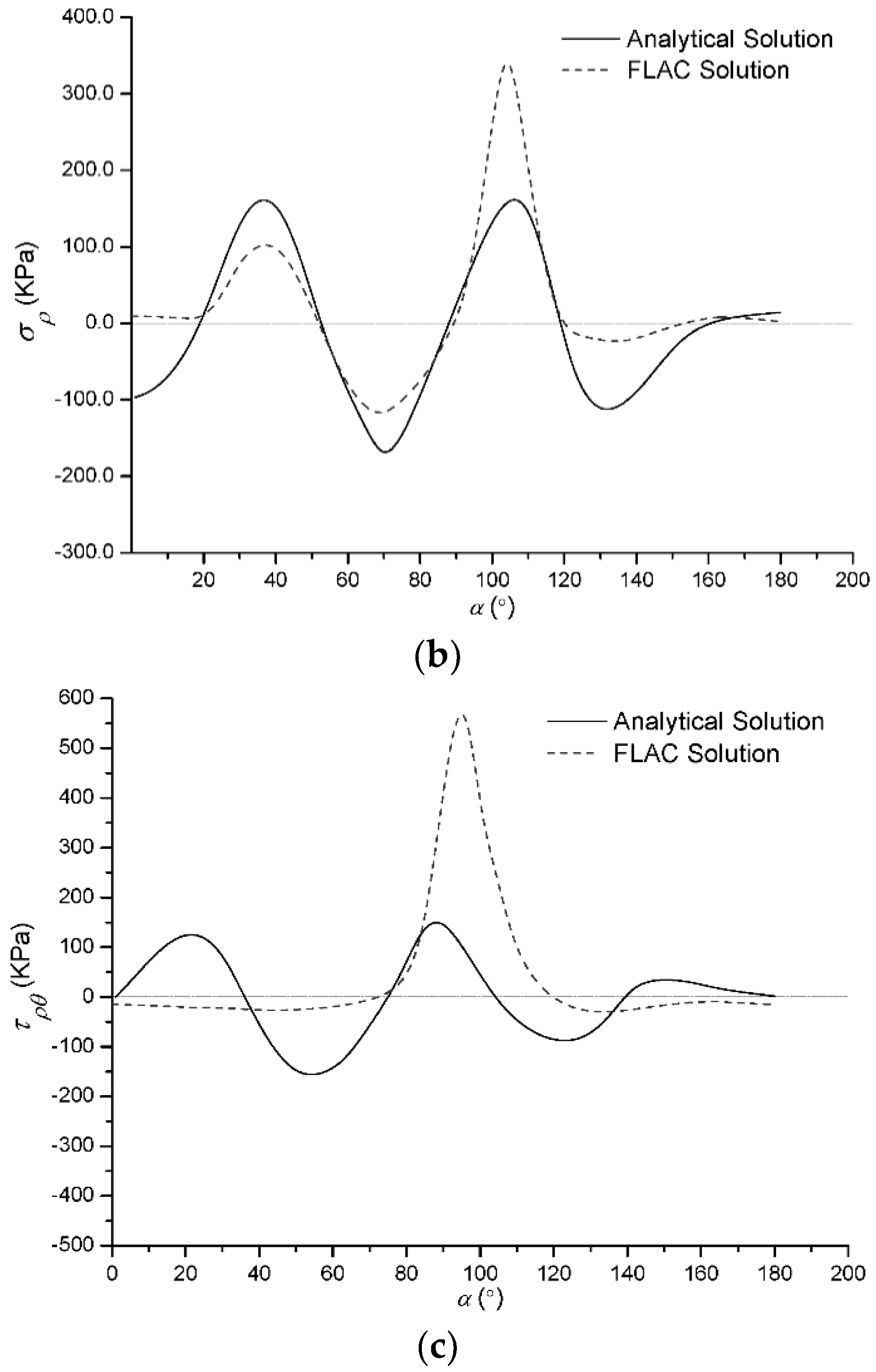
Figure 3 shows the circumferential stress along the rock–lining interface predicted by the new analytical solution and the FLAC finite difference software. It can be observed that the maximum circumferential stress happens at a position of an 85-degree angle (i.e., the widest part of the tunnel) and, moreover, the circumferential stress of the new analytical solution has not declined rapidly, but creates a stress concentration at $\mathsf{\alpha }=115°$. The circumferential stress along the inner lining periphery is presented in Figure 4a, demonstrating good agreement between the new analytical solution and the numerical simulation apart from an 85-degree angle. Normal stress and shear stress along the inner lining periphery is illustrated in Figure 4b,c; the maximum value of the analytical solution for normal stress and shear stress are about 200 KPa and 100 KPa, respectively, and the maximum value of the numerical simulation of normal stress and shear stress are about 350 KPa and 600 KPa. The analytical solution is smaller than the numerical simulation. The analytical solution is more accurate than the numerical simulation.

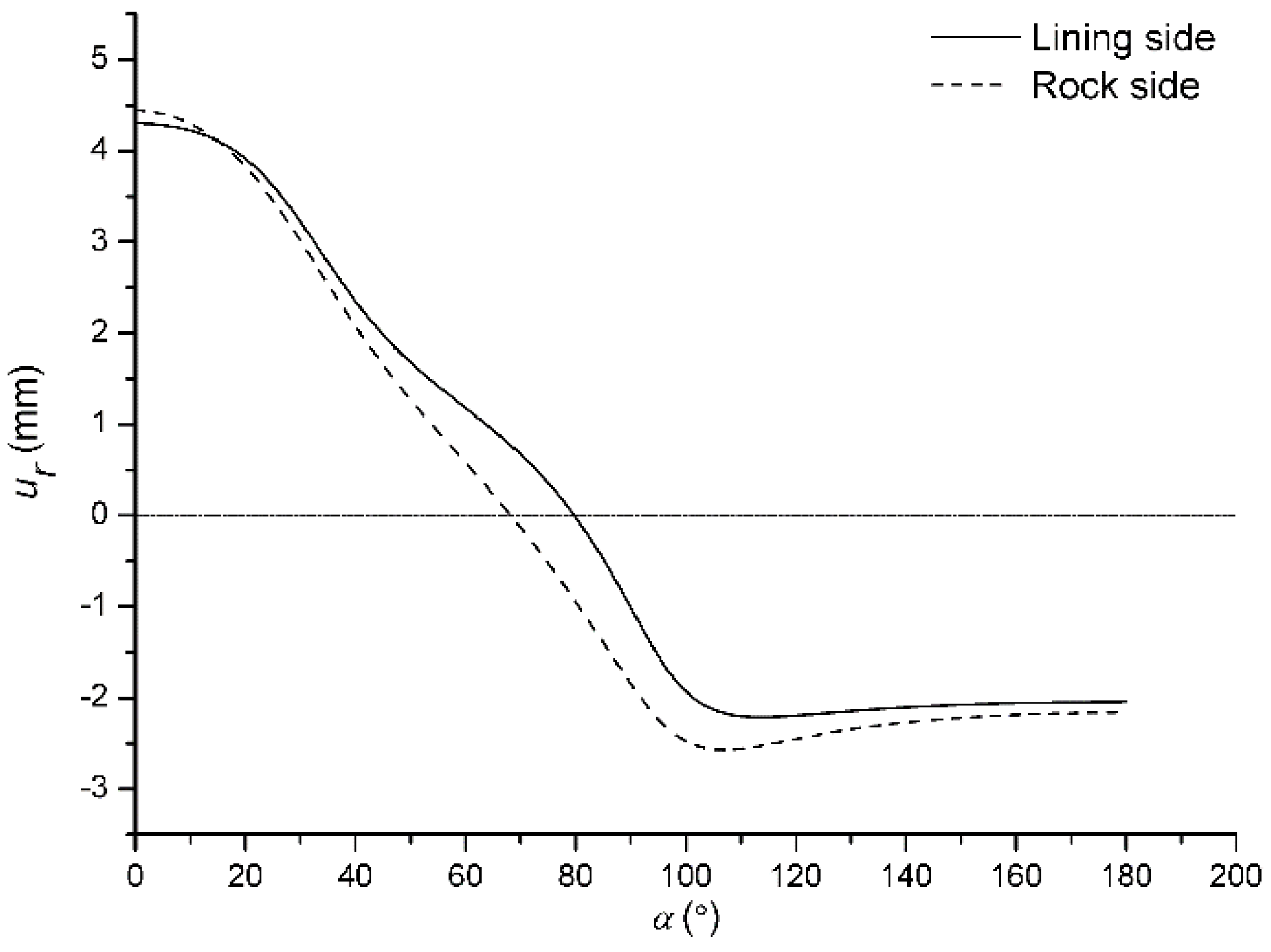
Figure 5 shows the radial displacement of the tunnel along the rock–lining interface predicted by the analytical solution. It could be demonstrated that the radial displacement along the rock–lining interface was in good agreement with the displacement boundary condition, which proves its high accuracy.

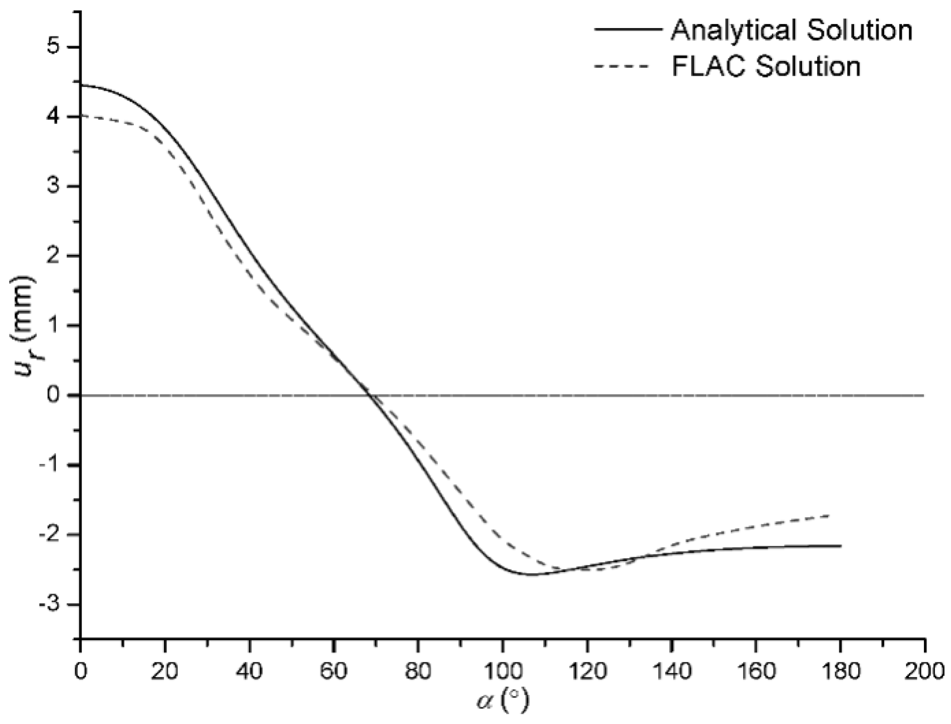
The radial displacement of the tunnel along the inner lining periphery is illustrated in Figure 6, which shows that the radial displacement of the analytical solution and numerical simulation are all zero at $\mathsf{\alpha }=75°$. It was demonstrated that the numerical solution agrees well with the analytical solution. Considering the results of Figure 5, the analytical solution had good agreement with the displacement boundary condition, thus the analytical solution results were reasonable.

The discrepancies between the new analytical solution and the numerical simulation described above, especially Figure 4, may be due to the fact that the grid size in the numerical modeling is not small enough to produce accurate results. The stress information of the numerical simulation is stored in zones not in grid points, and the stress cannot be accurately expressed along a specified boundary.

5. Conclusions

In this paper, the stress and displacement of a non-circular deep tunnel and within their lining supports were studied using a new analytical solution, which is based on the basic theory of complex variables and plane elasticity [17], and the following conclusions can be made.

The analytic functions were exactly established to predict the stress and displacement distribution of the non-circular deep tunnel within their lining supports, but it is obviously not entirely true that the stress and displacement value is only determined by the in-situ stress boundary conditions and coefficient of the elasticity modulus, Poisson’s ratio, lateral pressure and material density. The analytical solution for radial displacement was smaller than the numerical simulation results, however, and further study will be needed to develop these functions.

Due to the fact that the grid size in modeling was not small enough to produce accurate results and stress information was stored in zones, not in grid points in the numerical simulation, the stress cannot be accurately expressed along a specified boundary. But the analytical solution results were not affected by grid size and zones in the numerical modeling.

The curves of the stress value showed that the new analytical solution and numerical simulation were in reasonable agreement. Both solutions predicted a normal stress concentration at the lower and upper corners of the tunnel, and both maximum circumferential stress results occurred in the widest part of the tunnels. The normal and shear stress values of the tunnel along the inner lining periphery were almost zero, which proved its high accuracy.

Although numerical simulation is the main tool for solving tunnel excavation problems, especially non-circular tunnels, the complex variable method can provide another way to solve non-circular tunnel excavation problems in a faster and more accurate way.

References

- Bobet, A. Analytical solutions for shallow tunnels in saturated ground. J. Eng. Mech. 2001, 127, 1258–1266. [Google Scholar] [CrossRef]
- Bobet, A. Effect of pore water pressure on tunnel support during static and seismic loading. Tunn. Undergr. Space Technol. 2003, 18, 377–393. [Google Scholar] [CrossRef]
- Lee, I.M.; Nam, S.W. The study of seepage forces acting on the tunnel lining and tunnel face in shallow tunnels. Tunn. Undergr. Space Technol. 2001, 16, 31–40. [Google Scholar] [CrossRef]
- Timoshenko, S.P.; Goodier, J. Theory of Elasticity, 2nd ed.; McGraw-Hill: New York, NY, USA, 1951. [Google Scholar]
- Muskhelishvili, N.I.; Radok, J.R.M. Some Basic Problems of the Mathematical Theory of Elasticity; Cambridge University Press: Cambridge, UK, 1953. [Google Scholar]
- Exadaktylos, G.; Stavropoulou, M. A closed-form elastic solution for stresses and displacements around tunnels. Int. J. Rock Mech. Min. Sci. 2002, 39, 905–916. [Google Scholar] [CrossRef]
- Exadaktylos, G.E.; Liolios, P.A.; Stavropoulou, M.C. A semi-analytical elastic stress displacement solution for notched circular openings in rocks. Int. J. Solids Struct. 2003, 40, 1165–1187. [Google Scholar] [CrossRef]
- Verruijt, A. A complex variable solution for a deforming circular tunnel in an elastic half-plane. Int. J. Numer. Anal. Methods Geomech. 1997, 21, 77–89. [Google Scholar] [CrossRef]
- Verruijt, A. Deformations of an elastic half plane with a circular cavity. Int. J. Solids Struct. 1998, 35, 2795–2804. [Google Scholar] [CrossRef]
- Zhao, G.P.; Yang, S.L. Analytical solutions for rock stress around square tunnels using complex variable theory. Int. J. Rock Mech. Min. Sci. 2015, 80, 302–307. [Google Scholar] [CrossRef]
- Kargar, A.R.; Rahmannejad, R.; Hajabasi, M.A. A semi-analytical elastic solution for stress field of lined non-circular tunnels at great depth using complex variable method. Int. J. Solids Struct. 2014, 51, 1475–1482. [Google Scholar] [CrossRef]
- Li, Y.S.; Chen, S.G. A Complex Variable Solution for Stress and Deformation of Lining in a Non-Circular Tunnel. Scientific Research Report. Southwest Jiaotong University: Chengdu, China, 2018. (In Chinese) [Google Scholar]
- Liu, F.S. Seepage Studies of Tunnel Water-Enriched Region Based on Fluid-Solid Coupling Theory and Complex Analysis. Ph.D. Thesis, South China University, Guangzhou, China, 2012. (In Chinese). [Google Scholar]
- Wang, G.Q. Elastic Mechanics; China Railway Publishing House: Beijing, China, 2008. (In Chinese) [Google Scholar]
- Chen, Z.Y. Analytical Method in Mechanical Analysis of Surrounding Rock, 1st ed.; China Coal Industry Publishing House: Beijing, China, 1994. (In Chinese) [Google Scholar]
- Lv, Z.A.; Zhang, L.Q. Complex Function Method for Mechanical Analysis of Underground Tunnel, 1st ed.; Science Press: Beijing, China, 2007. (In Chinese) [Google Scholar]
- Brown, J.W.; Churchill, R.V. Complex Variables and Applications, 9th ed.; China Machine Press: Beijing, China, 2015. (In Chinese) [Google Scholar]
Figure 1.
Conformal mapping of the tunnel in the z-plane in to two concentric circles in the -plane.
Figure 2.
(a) Tunnel distribution diagram (Unit: m) and (b) Finite mesh calculation model.
Figure 3.
Circumferential stress along the rock–lining interface (a) from the lining side (b) from the rock side.
Figure 4.
Stress along the inner lining periphery (a) circumferential stress (b) normal stress (c) shear stress.
Figure 5.
Radial displacement along the rock–lining interface predicted by the analytical solution.
Figure 6.
Radial displacement along the inner lining periphery.