Specific Types of Pythagorean Fuzzy Graphs and Application to Decision-Making

Abstract

The purpose of this research study is to present some new operations, including rejection, symmetric difference, residue product, and maximal product of Pythagorean fuzzy graphs (PFGs), and to explore some of their properties. This research article introduces certain notions, including intuitionistic fuzzy graphs of 3-type (IFGs3T), intuitionistic fuzzy graphs of 4-type (IFGs4T), and intuitionistic fuzzy graphs of n-type (IFGsnT), and proves that every IFG(n − 1)T is an IFGnT (for $n\ge$ 2). Moreover, this study discusses the application of Pythagorean fuzzy graphs in decision making.

1. Introduction

Intuitionistic fuzzy sets (IFSs) [1] of first type, an extension of Zadeh’s notion of the fuzzy set [2] which itself extends the classical notion of a set, are sets whose elements have degrees of membership and non-membership. Yager [3,4] considered the Pythagorean fuzzy sets (PFSs) as a new generalization of IFSs which is characterized by the membership and the non-membership degree satisfying the condition that their square sum is not greater than 1. Some results for PFSs and the Pythagorean fuzzy TODIM approach to multi-criteria decision making have been presented in [5,6]. Zhang and Xu [7] dealt with the mathematical form of the PFS and introduced the concept of the Pythagorean fuzzy number (PFN). They also discussed a series of the basic operational laws of PFNs and proposed the Pythagorean fuzzy aggregation operators, including the Pythagorean fuzzy weighted averaging operator. The PFS is more general than the IFS because the space of PFSs’ membership degree is greater than the space of IFSs’ membership degree. For instance, when a decision-maker gives the evaluation information whose membership degree is 0.5 and non-membership degree is 0.8, it can be known that the IFN fails to address this issue because $0.5+0.8>1$. However, ${\left(0.5\right)}^2+{\left(0.8\right)}^2<1$. On the other hand, the notions of IFSs of second type (IFSs2T), IFSs of third type (IFSs3T), IFSs of fourth type (IFSs4T), and IFSs of n-th type (IFSsnT) have been studied in [8,9,10,11]. 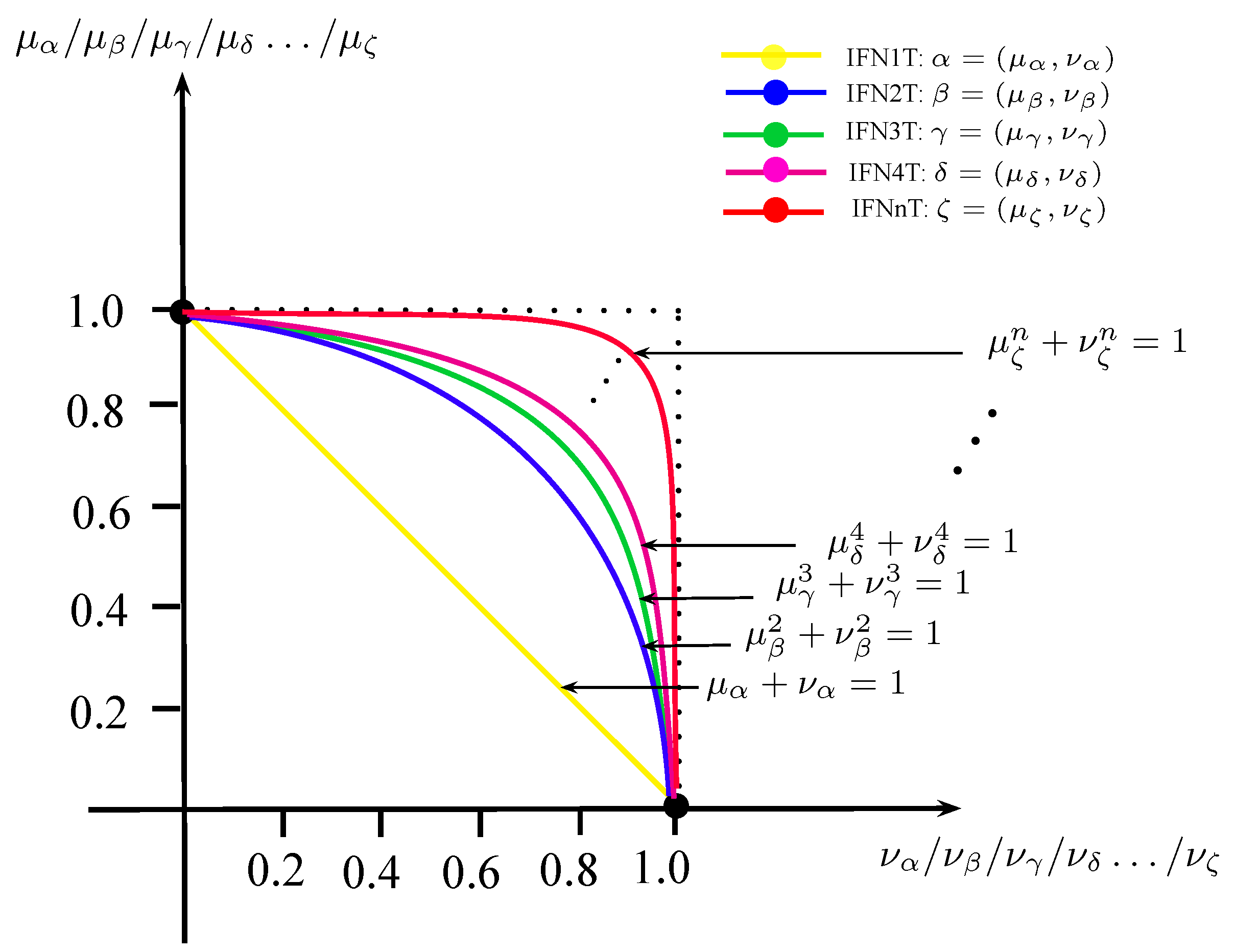For convenience, IFSnT is represented by IFNnT—that is, $\zeta =({\mu }_{\zeta },{\nu }_{\zeta }).$ The key difference between IFN1T, IFN2T, IFN3T, IFN4T, …, IFnNT is their different constraint conditions. That is, ${\mu }_{\alpha }+{\nu }_{\alpha }\le 1,{\mu }_{\beta }^2+{\nu }_{\beta }^2\le 1,{\mu }_{\gamma }^3+{\nu }_{\gamma }^3\le 1,{\mu }_{\delta }^4+{\nu }_{\delta }^4\le 1,\dots ,{\mu }_{\zeta }^n+{\nu }_{\zeta }^n\le 1$, respectively. The comparison of these spaces is shown in Figure 1. For other notation applications, readers are referred to [12,13,14,15,16,17,18,19,20].

A graph is a convenient way of interpreting information involving the relationship between objects. Fuzzy graphs are designed to represent the structures of relationships between objects such that the existence of a concrete object (vertex) and the relationship between two objects (edge) are matters of degree. The concept of fuzzy graphs was initiated by Kaufmann [21]. Later, Rosenfeld [22] discussed several theoretical concepts, including paths, cycles, and connectedness in fuzzy graphs. Mordeson and Peng [23] defined some operations on fuzzy graphs and investigated their properties. Parvathi and Karunambigai [24] considered intuitionistic fuzzy graphs (IFGs). Later, Akram and Davvaz [25] discussed IFGs. Akram and Dudek [26] described intuitionistic fuzzy hypergraphs with applications. Recently, Naz et al. [27] originally proposed the concept of Pythagorean fuzzy graphs(PFGs), a generalization of the notion of Akram and Davvaz’s IFGs [25], along with their applications in decision-making. Akram and Naz [28] studied the energy of PFGs with applications. Dhavudh and Srinivasan [29,30] dealt with IFGs2T. The graph operations perform a substantial role in many fields, especially in computer science. For example, the Cartesian product offers a significant model for linking computers. There are various operations on PFGs. Verma et al. [31] presented some operations of PFGs. In this research study, we present some new operations, including rejection, symmetric difference, residue product, and maximal product of PFGs (IFGs2T), which may be suggestive of some aspects of network design. We explore some of their properties, especially the degree of vertices, and total degree as its modification, of resultant PFGs, acquired from given PFGs using these operations. We introduce certain new notions, including IFGs3T, IFGs4T, and IFGsnT, and prove that every IFG(n − 1)T is an IFGnT (for $n\ge 2$). Moreover, we show that the definition and operations of PFGs (IFGs2T) mentioned in [29,31] contain some flaws. Finally, we discuss the application of PFGs in decision making.

2. Operations on Pythagorean Fuzzy Graphs

Definition 1.

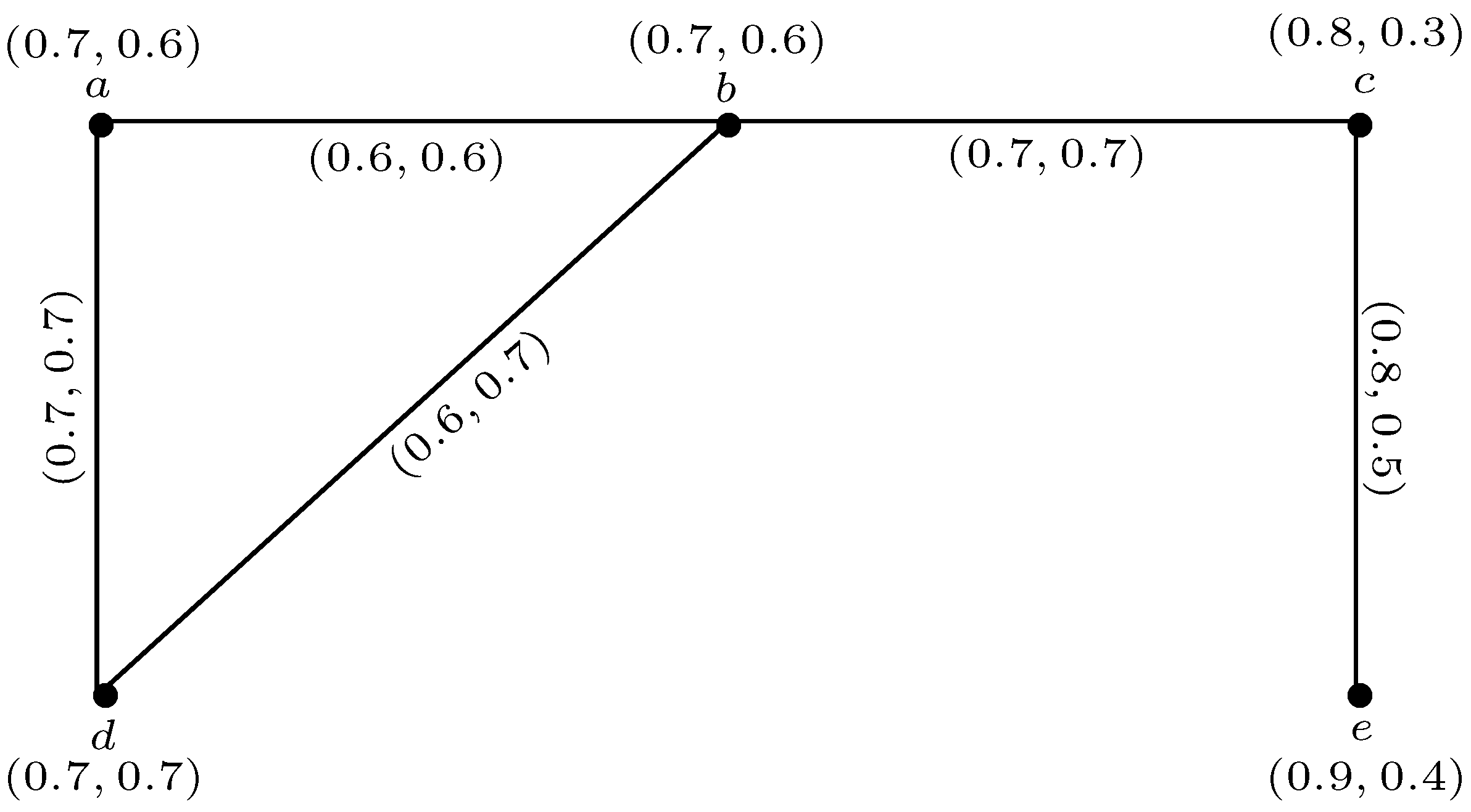
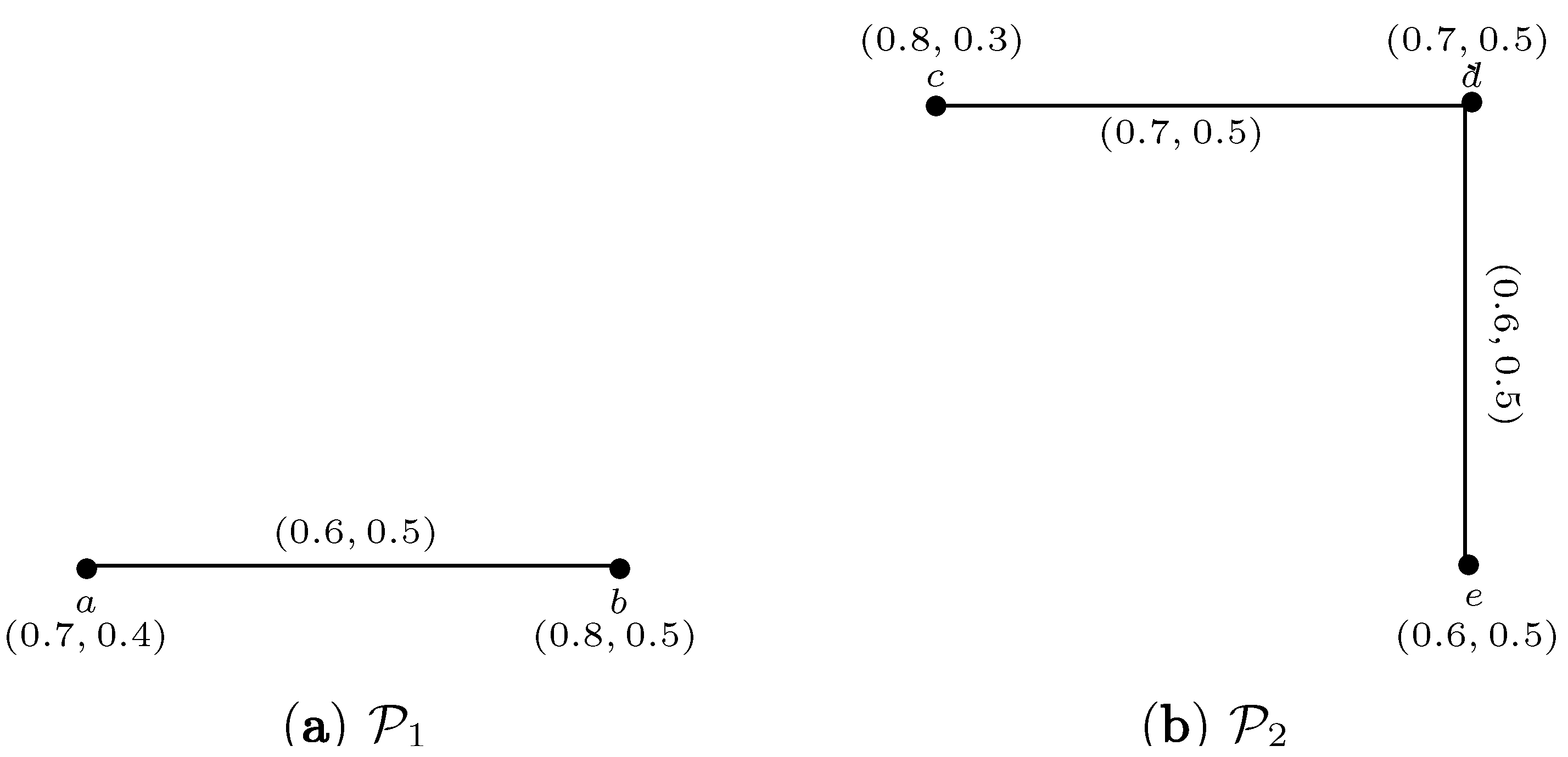
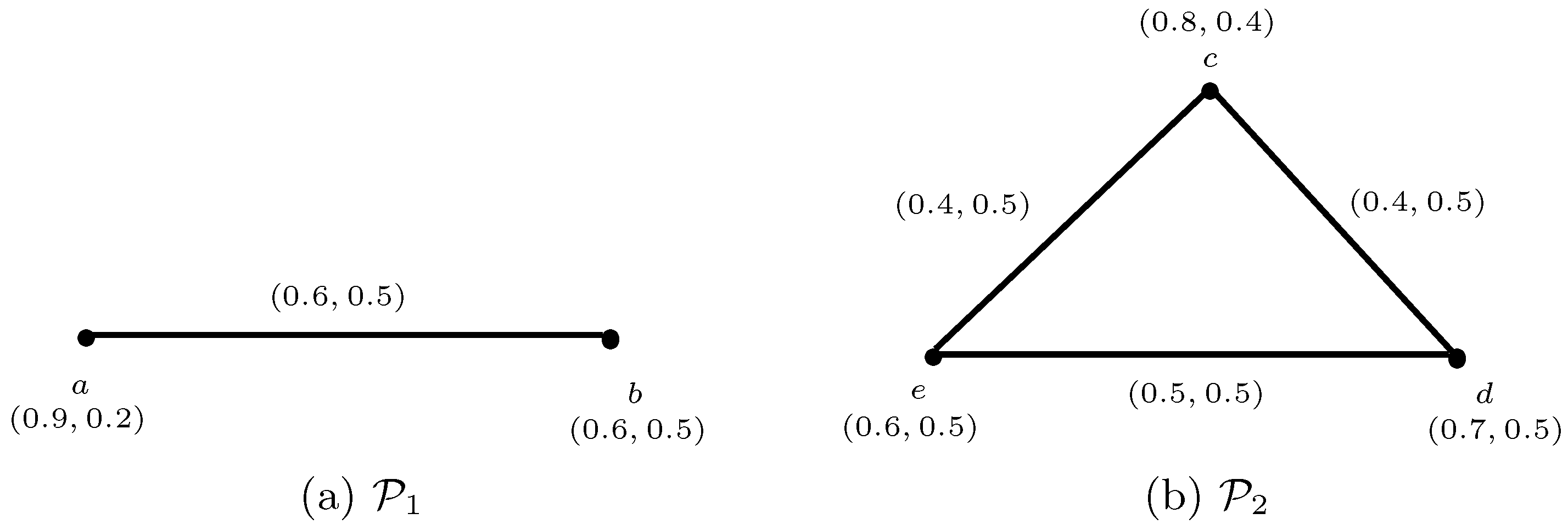
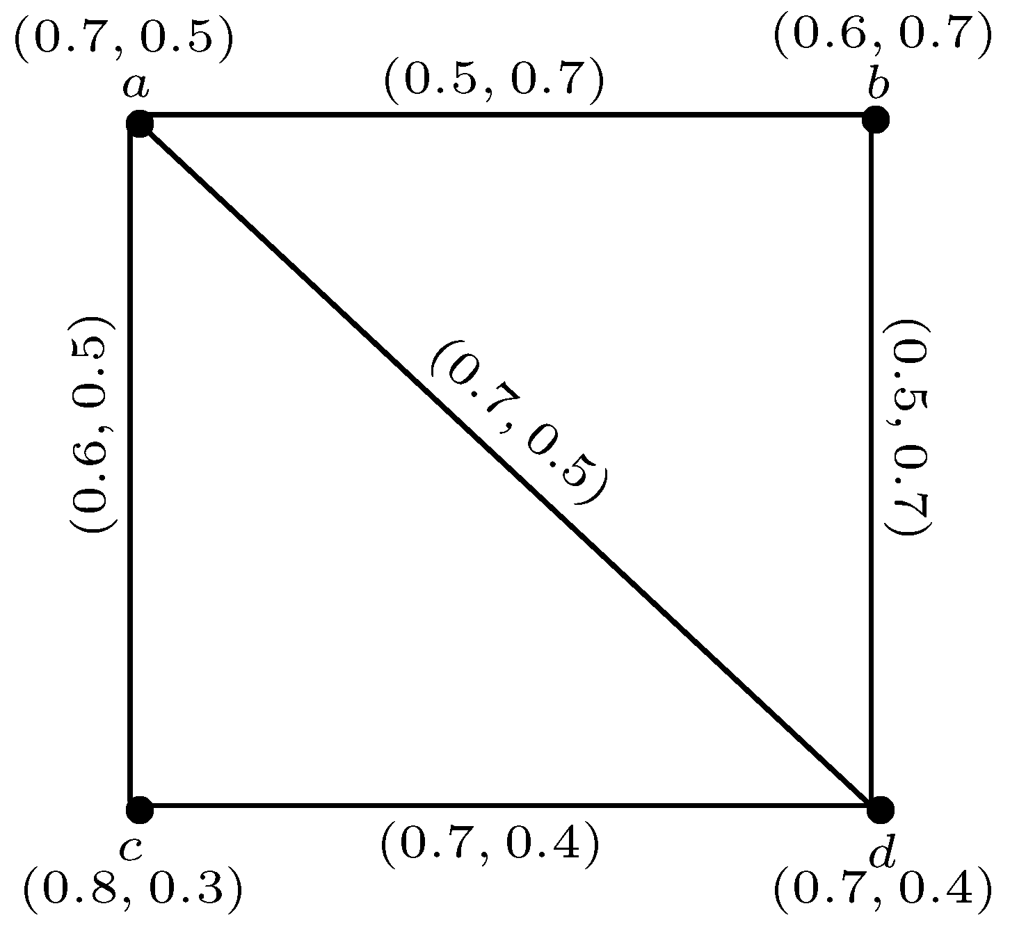
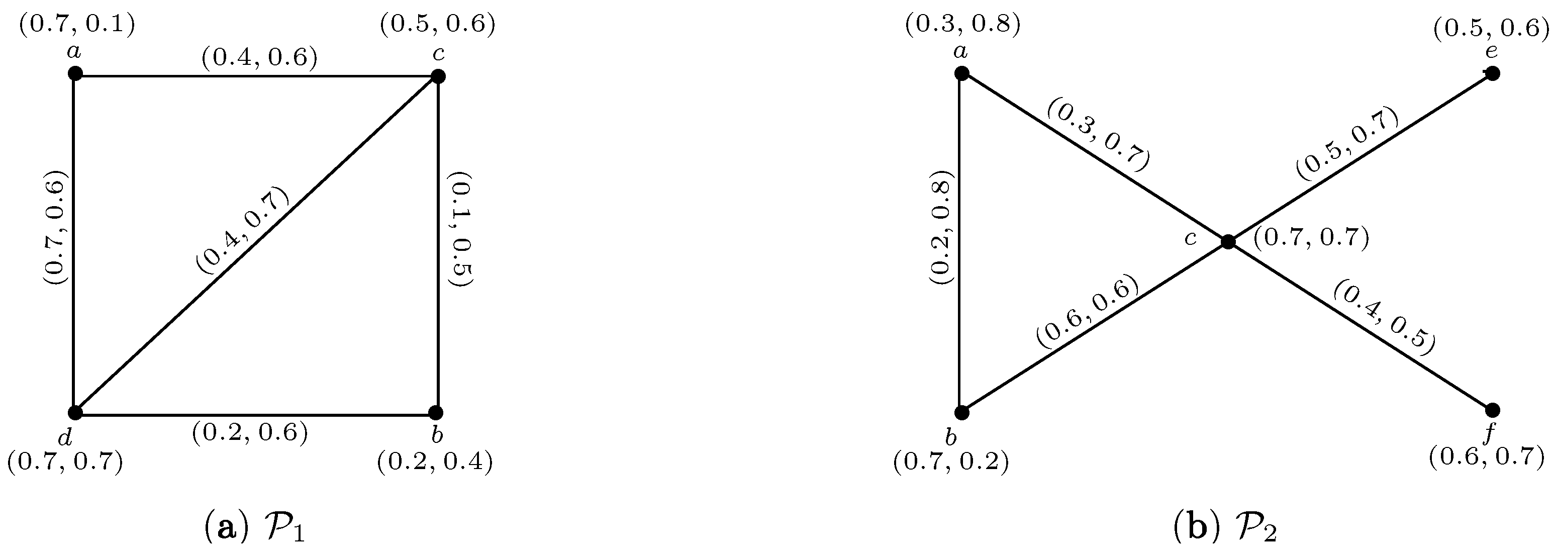
[27] A Pythagorean fuzzy graph (PFG) on a nonempty set V is a pair $\mathcal{P}=(\mathcal{C},\mathcal{D})$ with $\mathcal{C}$ a PFS on V and $\mathcal{D}$ a PFR on V such that

$${\mu }_{\mathcal{D}}\left(xy\right)\le {\mu }_{\mathcal{C}}\left(x\right)\wedge {\mu }_{\mathcal{C}}\left(y\right),{\nu }_{\mathcal{D}}\left(xy\right)\ge {\nu }_{\mathcal{C}}\left(x\right)\vee {\nu }_{\mathcal{C}}\left(y\right),$$

and $0\le {\mu }_{\mathcal{D}}^2\left(xy\right)+{\nu }_{\mathcal{D}}^2\left(xy\right)\le 1$ for all $x,y\in V$, where, ${\mu }_{\mathcal{D}}:V\times V⟶[0,1]$ and ${\nu }_{\mathcal{D}}:V\times V⟶[0,1]$ represent the membership and non-membership functions of $\mathcal{D}$, respectively. A PFG is also called an intuitionistic fuzzy graph of 2-type (IFG2T). For convenience, IFS2T(PFS) is represented by IFN2T(PFN) (i.e., $\beta =({\mu }_{\beta },{\nu }_{\beta })$).

Example 1.

Consider a simple graph $G=(V,E)$ such that $V=\{a,b,c,d,e\}andE=\{ab,bc,ad,bd,ce\}\subseteq V\times V.$ Let

$$\mathcal{C}=〈\left({\displaystyle \frac{a}{0.7}},{\displaystyle \frac{b}{0.7}},{\displaystyle \frac{c}{0.8}},{\displaystyle \frac{d}{0.7}},{\displaystyle \frac{e}{0.9}}\right),\left({\displaystyle \frac{a}{0.6}},{\displaystyle \frac{b}{0.6}},{\displaystyle \frac{c}{0.3}},{\displaystyle \frac{d}{0.7}},{\displaystyle \frac{e}{0.4}}\right)〉 \mathit{and}$$

$$\mathcal{D}=〈\left({\displaystyle \frac{ab}{0.6}},{\displaystyle \frac{bc}{0.7}},{\displaystyle \frac{ad}{0.7}},{\displaystyle \frac{bd}{0.6}},{\displaystyle \frac{ce}{0.8}}\right),\left({\displaystyle \frac{ab}{0.6}},{\displaystyle \frac{bc}{0.7}},{\displaystyle \frac{ad}{0.7}},{\displaystyle \frac{bd}{0.7}},{\displaystyle \frac{ce}{0.5}}\right)〉$$

be the Pythagorean fuzzy vertex set and the Pythagorean fuzzy edge set defined on V and E, respectively. By direct calculations, it is easy to see from Figure 2 that $\mathcal{P}=(\mathcal{C},\mathcal{D})$ is a PFG (IFG2T).

Definition 2.

Let ${\mathcal{P}}_1=({\mathcal{C}}_1,{\mathcal{D}}_1)$ and ${\mathcal{P}}_2=({\mathcal{C}}_2,{\mathcal{D}}_2)$ be two PFGs of the graphs $G_1=(V_1,E_1)$ and $G_2=(V_2,E_2)$, respectively. The rejection of ${\mathcal{P}}_1$ and ${\mathcal{P}}_2$ is denoted by ${\mathcal{P}}_1|{\mathcal{P}}_2=({\mathcal{C}}_1|{\mathcal{C}}_2,{\mathcal{D}}_1\left|{\mathcal{D}}_2\right)$ and defined as:

(i)

$\left\{\begin{array}{c}\left({\mu }_{{\mathcal{C}}_1}\right|{\mu }_{{\mathcal{C}}_2})(x_1,x_2)={\mu }_{{\mathcal{C}}_1}\left(x_1\right)\wedge {\mu }_{{\mathcal{C}}_2}\left(x_2\right)\hfill \\ \left({\nu }_{{\mathcal{C}}_1}\right|{\nu }_{{\mathcal{C}}_2})(x_1,x_2)={\nu }_{{\mathcal{C}}_1}\left(x_1\right)\vee {\nu }_{{\mathcal{C}}_2}\left(x_2\right)\hfill \end{array}\right.$

for all $(x_1,x_2)\in V_1\times V_2,$

(ii)

$\left\{\begin{array}{c}\left({\mu }_{{\mathcal{D}}_1}\right|{\mu }_{{\mathcal{D}}_2})\left((x,x_2)(x,y_2)\right)={\mu }_{{\mathcal{C}}_1}\left(x\right)\wedge {\mu }_{{\mathcal{C}}_2}\left(x_2\right)\wedge {\mu }_{{\mathcal{C}}_2}\left(y_2\right)\hfill \\ \left({\nu }_{{\mathcal{D}}_1}\right|{\nu }_{{\mathcal{D}}_2})\left((x,x_2)(x,y_2)\right)={\nu }_{{\mathcal{C}}_1}\left(x\right)\vee {\nu }_{{\mathcal{C}}_2}\left(x_2\right)\vee {\nu }_{{\mathcal{C}}_2}\left(y_2\right)\hfill \end{array}\right.$

for all $x\in V_1$, $x_2{y}_2\notin E_2,$

(iii)

$\left\{\begin{array}{c}\left({\mu }_{{\mathcal{D}}_1}\right|{\mu }_{{\mathcal{D}}_2})\left((x_1,z)(y_1,z)\right)={\mu }_{{\mathcal{C}}_1}\left(x_1\right)\wedge {\mu }_{{\mathcal{C}}_1}\left(y_1\right)\wedge {\mu }_{{\mathcal{C}}_2}\left(z\right)\hfill \\ \left({\nu }_{{\mathcal{D}}_1}\right|{\nu }_{{\mathcal{D}}_2})\left((x_1,z)(y_1,z)\right)={\nu }_{{\mathcal{C}}_1}\left(x_1\right)\vee {\nu }_{{\mathcal{C}}_1}\left(y_1\right)\vee {\nu }_{{\mathcal{C}}_2}\left(z\right)\hfill \end{array}\right.$

for all $z\in V_2$ and $x_1{y}_1\notin E_1,$

(iv)

$\left\{\begin{array}{c}\left({\mu }_{{\mathcal{D}}_1}\right|{\mu }_{{\mathcal{D}}_2})\left((x_1,x_2)(y_1,y_2)\right)={\mu }_{{\mathcal{C}}_1}\left(x_1\right)\wedge {\mu }_{{\mathcal{C}}_1}\left(y_1\right)\wedge {\mu }_{{\mathcal{C}}_2}\left(x_2\right)\wedge {\mu }_{{\mathcal{C}}_2}\left(y_2\right)\hfill \\ \left({\nu }_{{\mathcal{D}}_1}\right|{\nu }_{{\mathcal{D}}_2})\left((x_1,x_2)(y_1,y_2)\right)={\nu }_{{\mathcal{C}}_1}\left(x_1\right)\vee {\nu }_{{\mathcal{C}}_1}\left(y_1\right)\vee {\nu }_{{\mathcal{C}}_2}\left(x_2\right)\vee {\nu }_{{\mathcal{C}}_2}\left(y_2\right)\hfill \end{array}\right.$

for all $x_1{y}_1\notin E_1$ and $x_2{y}_2\notin E_2.$

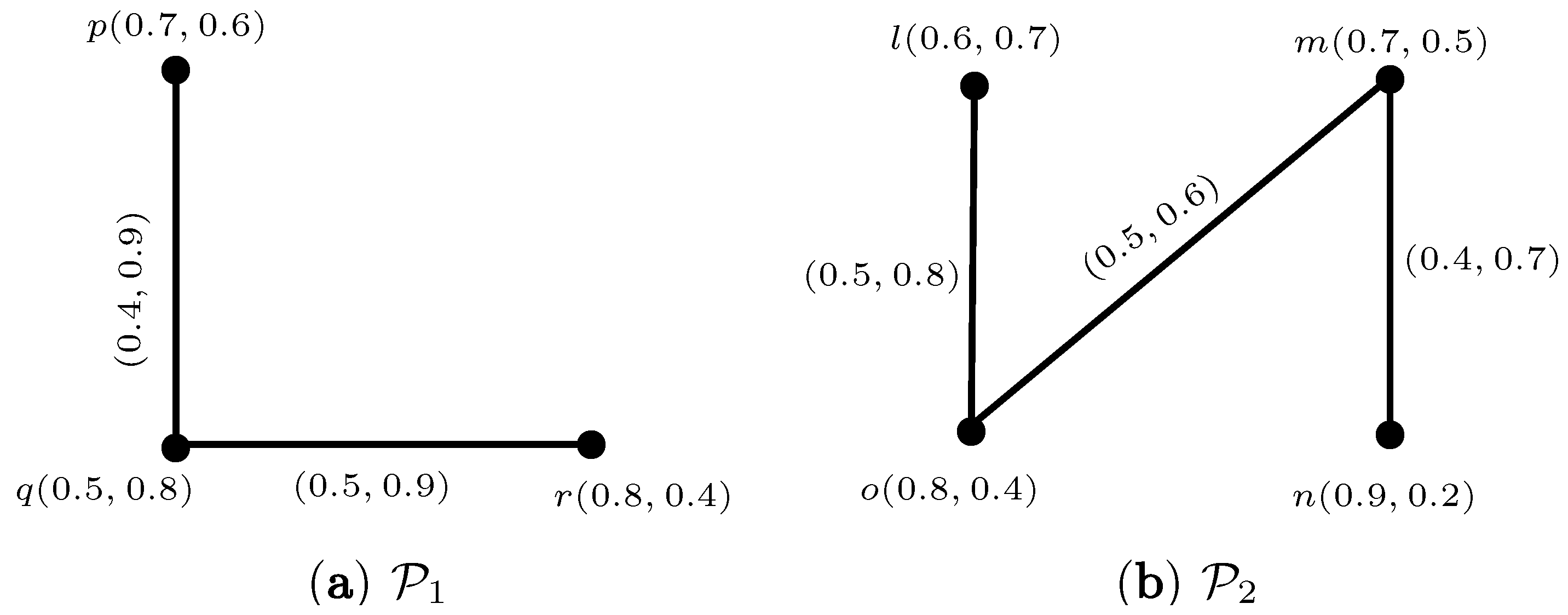
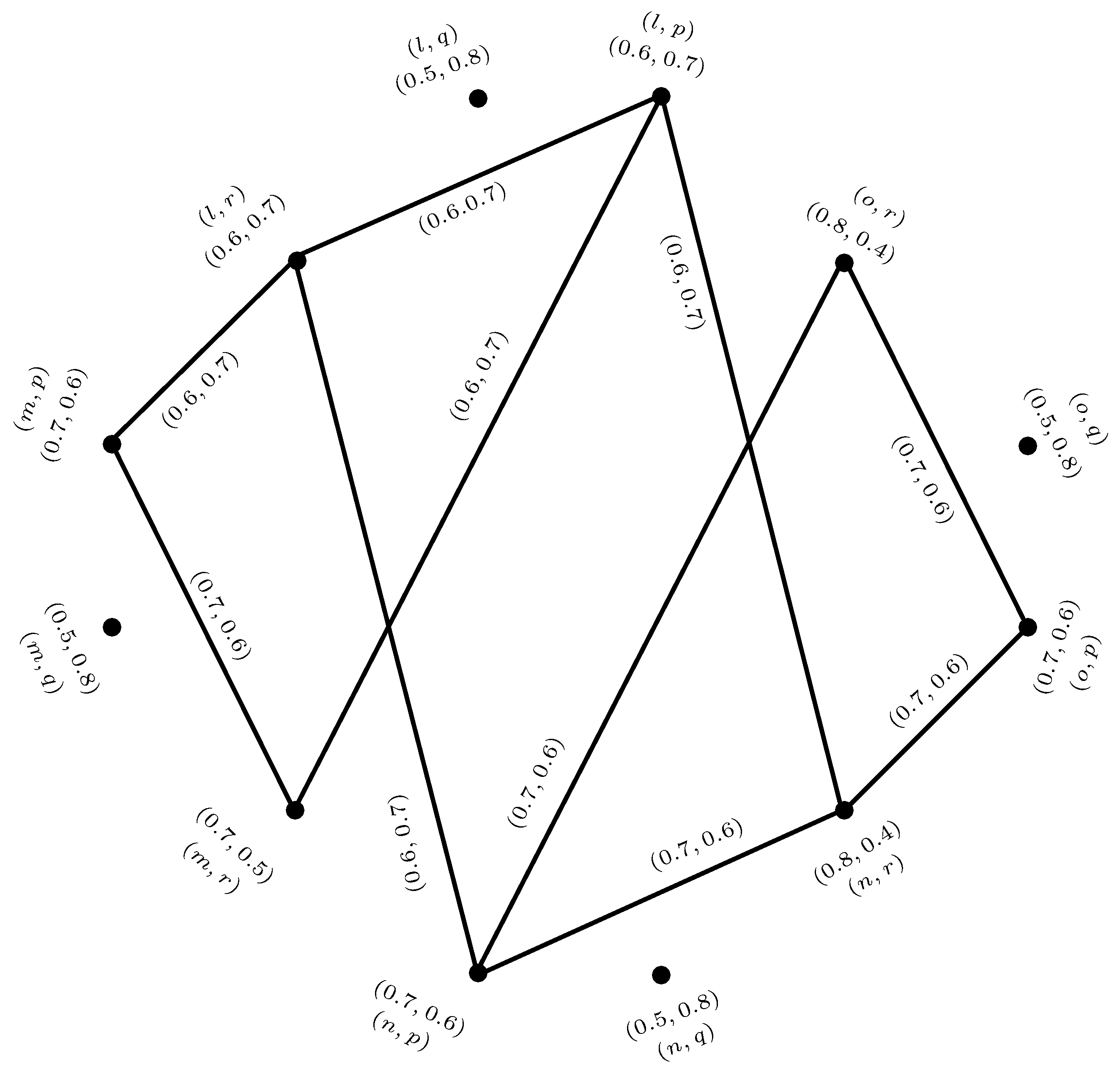
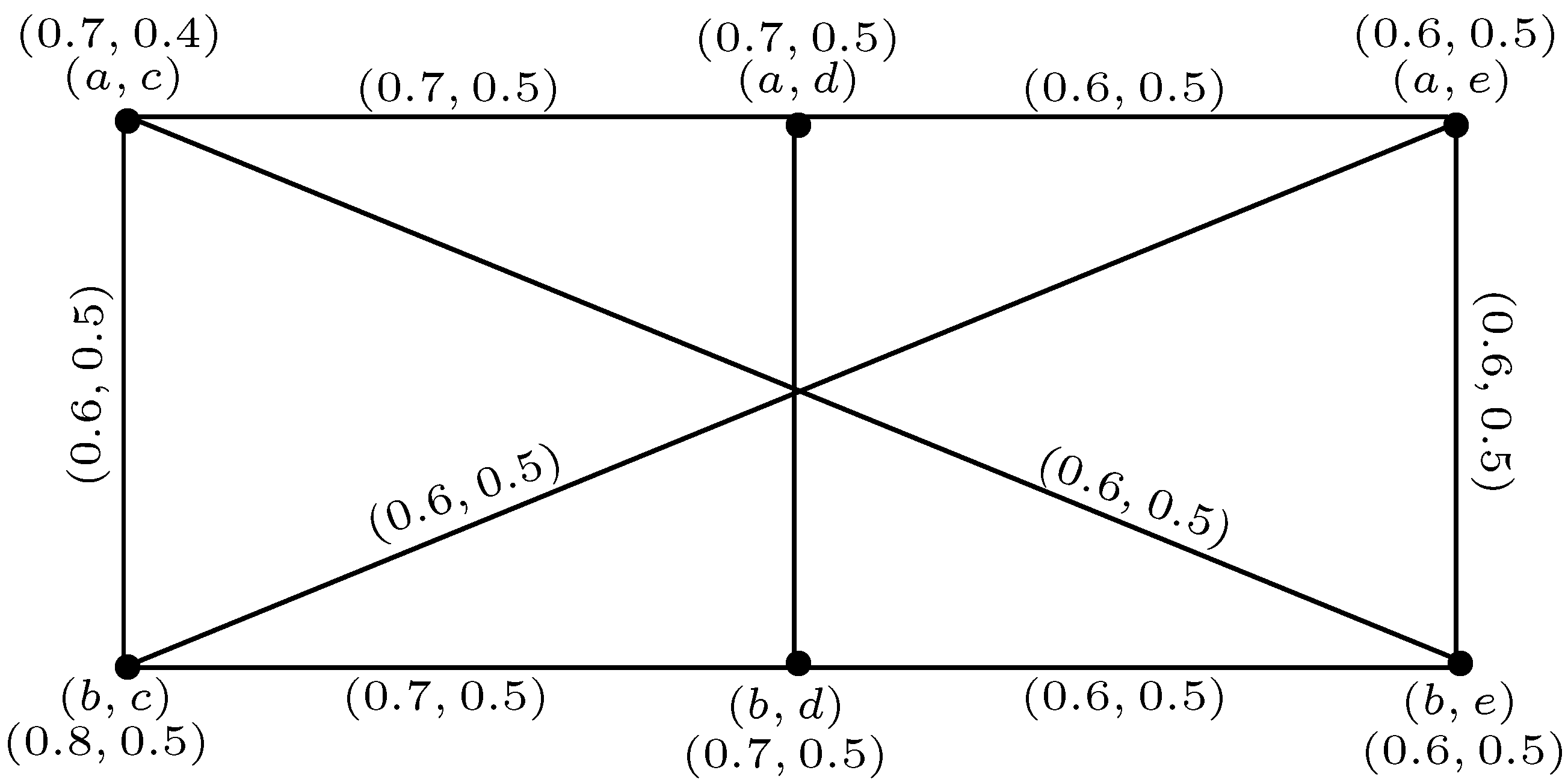
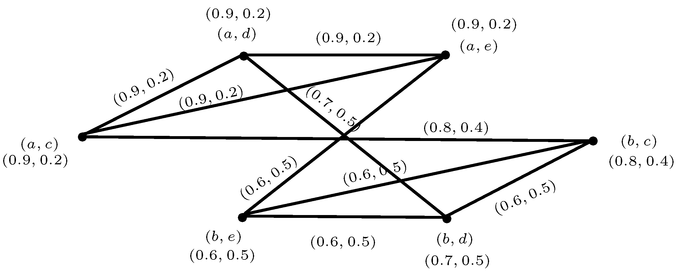
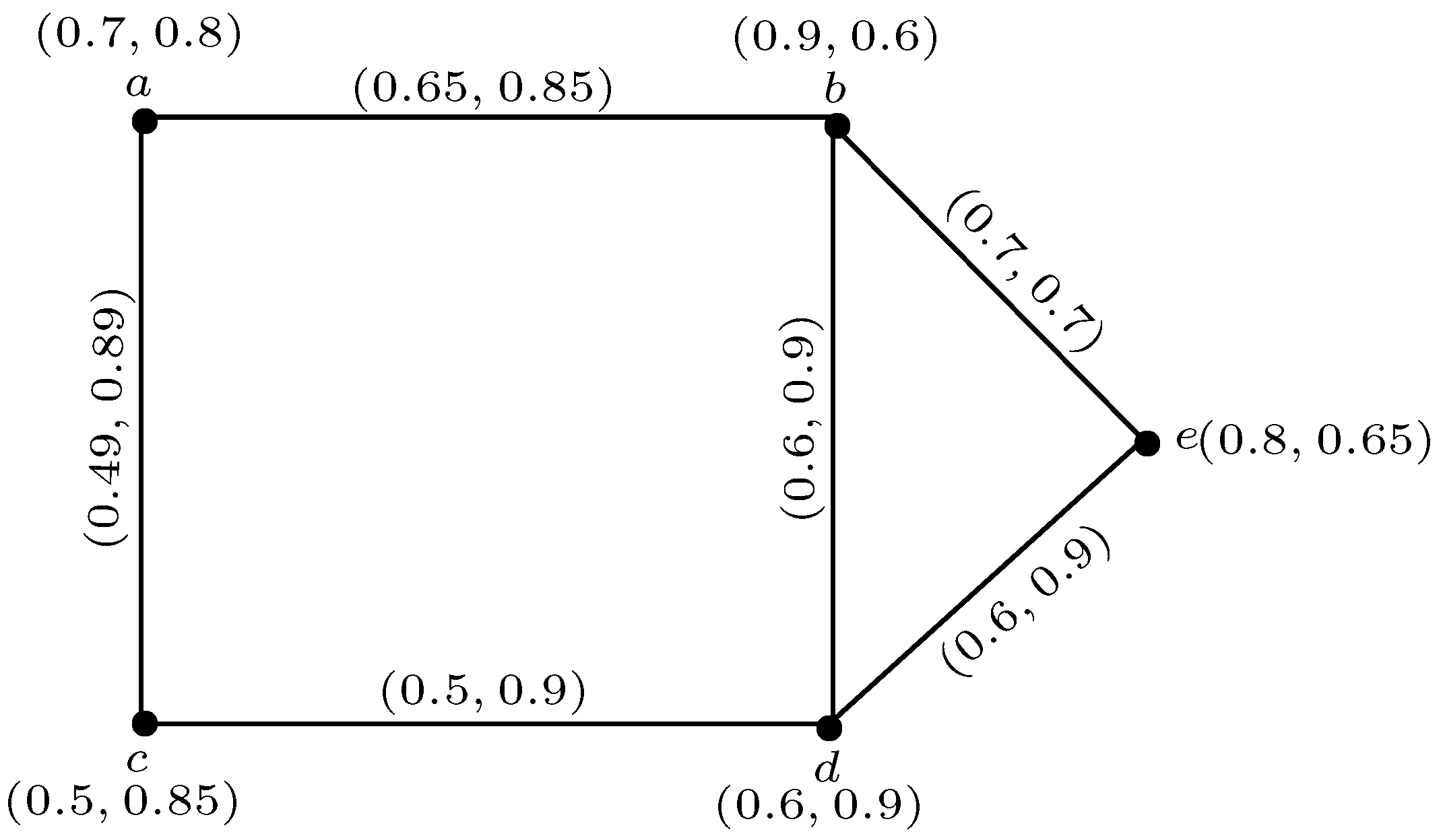
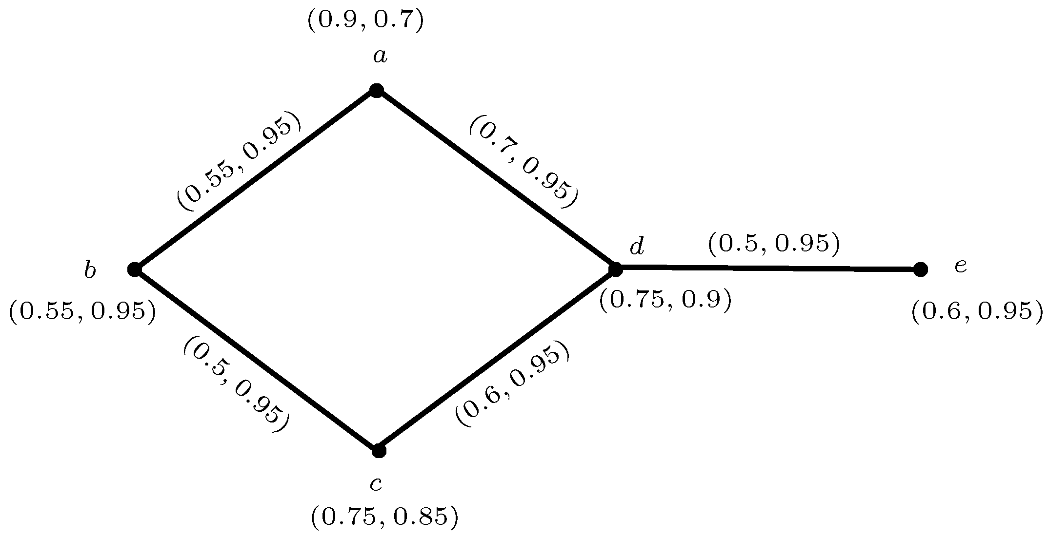
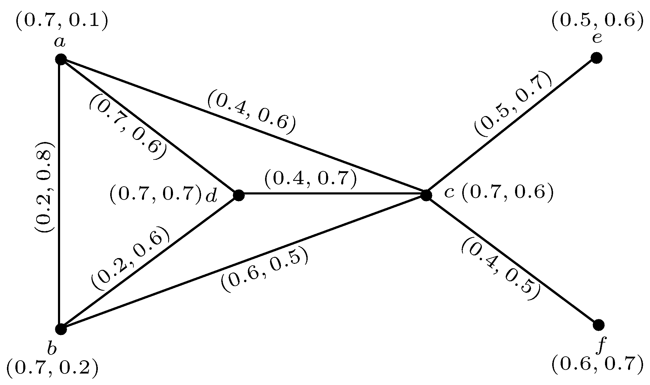
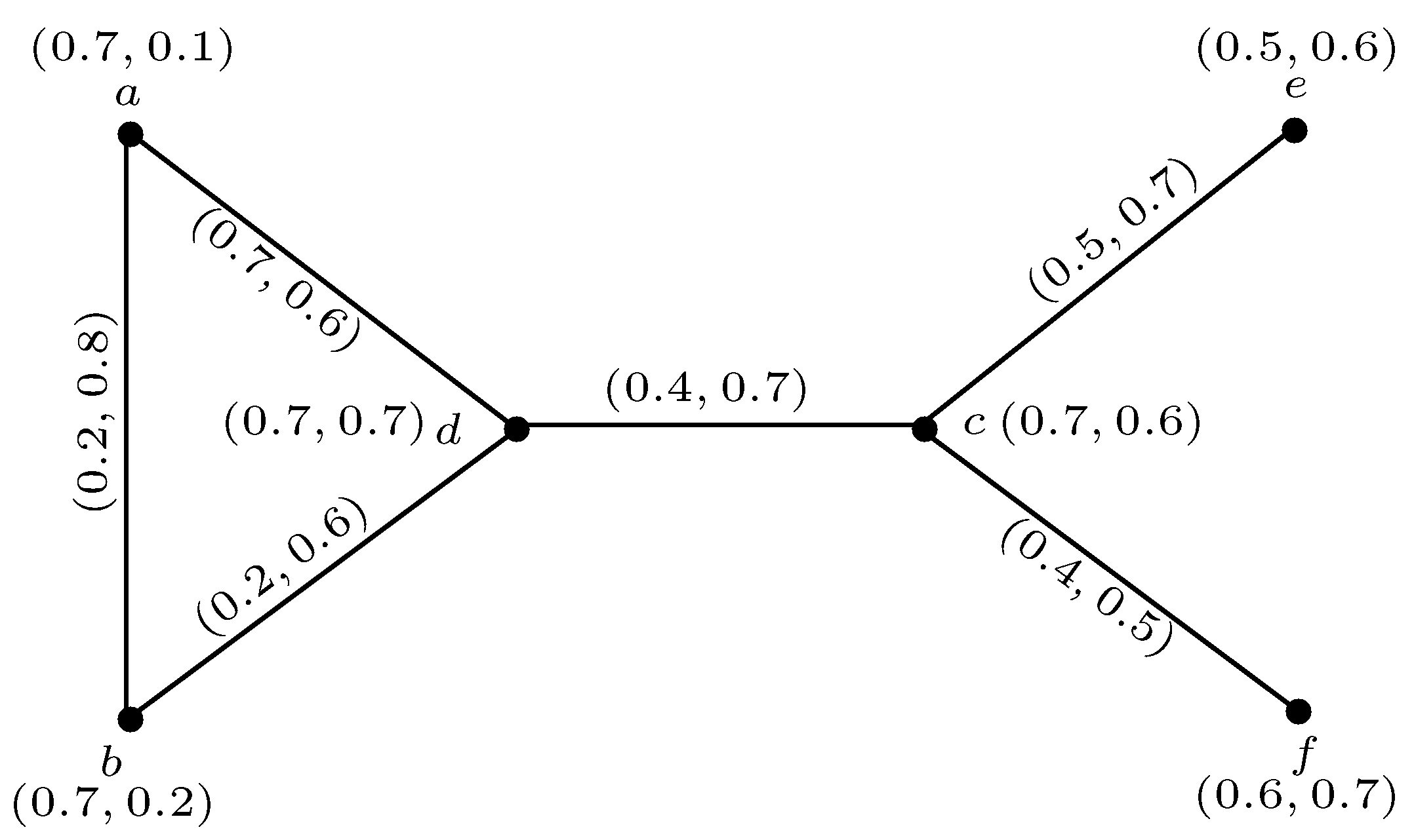
Example 2.

Consider two PFGs ${\mathcal{P}}_1=({\mathcal{C}}_1,{\mathcal{D}}_1)$ and ${\mathcal{P}}_2=({\mathcal{C}}_2,{\mathcal{D}}_2)$ on $V_1=\{l,m,n,o\}$ and $V_2=\{p,q,r\}$, respectively, as shown in Figure 3. Their rejection ${\mathcal{P}}_1|{\mathcal{P}}_2$ is shown in Figure 4.

Proposition 1.

Let ${\mathcal{P}}_1$ and ${\mathcal{P}}_2$ be the PFGs of the graphs $G_1$ and $G_2$, respectively. The rejection ${\mathcal{P}}_1|{\mathcal{P}}_2$ of ${\mathcal{P}}_1$ and ${\mathcal{P}}_2$ is a PFG.

Proof. 

Let ${\mathcal{P}}_1=({\mathcal{C}}_1,{\mathcal{D}}_1)$ and ${\mathcal{P}}_2=({\mathcal{C}}_1,{\mathcal{D}}_1)$ be the PFGs of the graphs $G_1=(V_1,E_1)$ and $G_2=(V_2,E_2)$, respectively. Then, for $(x_1,x_2)(y_1,y_2)\in E_1\times E_2$,

If $x_1=y_1$, $x_2{y}_2\notin E_2$,

$$\begin{array}{ccc}\hfill \left({\mu }_{{\mathcal{D}}_1}\right|{\mu }_{{\mathcal{D}}_2})\left((x_1,x_2)(y_1,y_2)\right)& =& {\mu }_{{\mathcal{C}}_1}\left(x_1\right)\wedge {\mu }_{{\mathcal{C}}_2}\left(x_2\right)\wedge {\mu }_{{\mathcal{C}}_2}\left(y_2\right)\hfill \\ & =& \{{\mu }_{{\mathcal{C}}_1}\left(x_1\right)\wedge {\mu }_{{\mathcal{C}}_2}\left(x_2\right)\}\wedge \{{\mu }_{{\mathcal{C}}_1}\left(y_1\right)\wedge {\mu }_{{\mathcal{C}}_2}\left(y_2\right)\}\hfill \\ & =& \left({\mu }_{{\mathcal{C}}_1}\right|{\mu }_{{\mathcal{C}}_2})(x_1,x_2)\wedge \left({\mu }_{{\mathcal{C}}_1}\right|{\mu }_{{\mathcal{C}}_2})(y_1,y_2),\hfill \end{array}$$

$$\begin{array}{ccc}\hfill \left({\nu }_{{\mathcal{D}}_1}\right|{\nu }_{{\mathcal{D}}_2})\left((x_1,x_2)(y_1,y_2)\right)& =& {\nu }_{{\mathcal{C}}_1}\left(x_1\right)\vee {\nu }_{{\mathcal{C}}_2}\left(x_2\right)\vee {\nu }_{{\mathcal{C}}_2}\left(y_2\right)\hfill \\ & =& \{{\nu }_{{\mathcal{C}}_1}\left(x\right)\vee {\nu }_{{\mathcal{C}}_2}\left(x_2\right)\}\vee \{{\nu }_{{\mathcal{C}}_1}\left(y_1\right)\vee {\nu }_{{\mathcal{C}}_2}\left(y_2\right)\}\hfill \\ & =& \left({\nu }_{{\mathcal{C}}_1}\right|{\nu }_{{\mathcal{C}}_2})(x_1,x_2)\vee \left({\nu }_{{\mathcal{C}}_1}\right|{\nu }_{{\mathcal{C}}_2})(y_1,y_2).\hfill \end{array}$$

If $x_2=y_2$, $x_1{y}_1\notin E_1$,

$$\begin{array}{ccc}\hfill \left({\mu }_{{\mathcal{D}}_1}\right|{\mu }_{{\mathcal{D}}_2})\left((x_1,x_2)(y_1,y_2)\right)& =& {\mu }_{{\mathcal{C}}_1}\left(x_1\right)\wedge {\mu }_{{\mathcal{C}}_1}\left(y_1\right)\wedge {\mu }_{{\mathcal{C}}_2}\left(x_2\right)\hfill \\ & =& \{{\mu }_{{\mathcal{C}}_1}\left(x_1\right)\wedge {\mu }_{{\mathcal{C}}_2}\left(x_2\right)\}\wedge \{{\mu }_{{\mathcal{C}}_1}\left(y_1\right)\wedge {\mu }_{{\mathcal{C}}_2}\left(y_2\right)\}\hfill \\ & =& \left({\mu }_{{\mathcal{C}}_1}\right|{\mu }_{{\mathcal{C}}_2})(x_1,x_2)\wedge \left({\mu }_{{\mathcal{C}}_1}\right|{\mu }_{{\mathcal{C}}_2})(y_1,y_2),\hfill \end{array}$$

$$\begin{array}{ccc}\hfill \left({\nu }_{{\mathcal{D}}_1}\right|{\nu }_{{\mathcal{D}}_2})\left((x_1,x_2)(y_1,y_2)\right)& =& {\nu }_{{\mathcal{C}}_1}\left(x_1\right)\vee {\nu }_{{\mathcal{C}}_1}\left(y_1\right)\vee {\nu }_{{\mathcal{C}}_2}\left(x_2\right)\hfill \\ & =& \{{\nu }_{{\mathcal{C}}_1}\left(x_1\right)\vee {\nu }_{{\mathcal{C}}_2}\left(x_2\right)\}\vee \{{\nu }_{{\mathcal{C}}_1}\left(y_1\right)\vee {\nu }_{{\mathcal{C}}_2}\left(y_2\right)\}\hfill \\ & =& \left({\nu }_{{\mathcal{C}}_1}\right|{\nu }_{{\mathcal{C}}_2})(x_1,x_2)\vee \left({\nu }_{{\mathcal{C}}_1}\right|{\nu }_{{\mathcal{C}}_2})(y_1,y_2).\hfill \end{array}$$

If $x_1{y}_1\notin E_1$, $x_2{y}_2\notin E_2$,

$$\begin{array}{ccc}\hfill \left({\mu }_{{\mathcal{D}}_1}\right|{\mu }_{{\mathcal{D}}_2})\left((x_1,x_2)(y_1,y_2)\right)& =& {\mu }_{{\mathcal{C}}_1}\left(x_1\right)\wedge {\mu }_{{\mathcal{C}}_1}\left(y_1\right)\wedge {\mu }_{{\mathcal{C}}_2}\left(x_2\right)\wedge {\mu }_{{\mathcal{C}}_1}\left(y_2\right)\hfill \\ & =& \{{\mu }_{{\mathcal{C}}_1}\left(x_1\right)\wedge {\mu }_{{\mathcal{C}}_2}\left(x_2\right)\}\wedge \{{\mu }_{{\mathcal{C}}_1}\left(y_1\right)\wedge {\mu }_{{\mathcal{C}}_2}\left(y_2\right)\}\hfill \\ & =& \left({\mu }_{{\mathcal{C}}_1}\right|{\mu }_{{\mathcal{C}}_2})(x_1,x_2)\wedge \left({\mu }_{{\mathcal{C}}_1}\right|{\mu }_{{\mathcal{C}}_2})(y_1,y_2),\hfill \end{array}$$

$$\begin{array}{ccc}\hfill \left({\nu }_{{\mathcal{D}}_1}\right|{\nu }_{{\mathcal{D}}_2})\left((x_1,x_2)(y_1,y_2)\right)& =& {\nu }_{{\mathcal{C}}_1}\left(x_1\right)\vee {\nu }_{{\mathcal{C}}_1}\left(y_1\right)\vee {\nu }_{{\mathcal{C}}_2}\left(x_2\right)\vee {\nu }_{{\mathcal{C}}_1}\left(y_2\right)\hfill \\ & =& \{{\nu }_{{\mathcal{C}}_1}\left(x_1\right)\vee {\nu }_{{\mathcal{C}}_2}\left(x_2\right)\}\vee \{{\nu }_{{\mathcal{C}}_1}\left(y_1\right)\vee {\nu }_{{\mathcal{C}}_2}\left(y_2\right)\}\hfill \\ & =& \left({\nu }_{{\mathcal{C}}_1}\right|{\nu }_{{\mathcal{C}}_2})(x_1,x_2)\vee \left({\nu }_{{\mathcal{C}}_1}\right|{\nu }_{{\mathcal{C}}_2})(y_1,y_2).\hfill \end{array}$$

Hence, from all cases it is clear that ${\mathcal{D}}_1|{\mathcal{D}}_2$ is a PFR on ${\mathcal{C}}_1|{\mathcal{C}}_2$. Hence, ${\mathcal{P}}_1|{\mathcal{P}}_2=({\mathcal{C}}_1|{\mathcal{C}}_2,{\mathcal{D}}_1\left|{\mathcal{D}}_2\right)$ is a PFG. ☐

Definition 3.

Let ${\mathcal{P}}_1=({\mathcal{C}}_1,{\mathcal{D}}_1)$ and ${\mathcal{P}}_2=({\mathcal{C}}_2,{\mathcal{D}}_2)$ be two PFGs. For any vertex $(x_1,x_2)\in V_1\times V_2$,

$$\begin{array}{c}\hfill \begin{array}{cc}\hfill {\left(d_{\mu }\right)}_{{\mathcal{P}}_1|{\mathcal{P}}_2}(x_1,x_2)& =\sum _{(x_1,x_2)(y_1,y_2)\in E_1\times E_2}\left({\mu }_{{\mathcal{D}}_1}\right|{\mu }_{{\mathcal{D}}_2})\left((x_1,x_2)(y_1,y_2)\right)\hfill \\ & =\sum _{x_1=y_1,x_2{y}_2\notin E_2}{\mu }_{{\mathcal{C}}_1}\left(x_1\right)\wedge {\mu }_{{\mathcal{C}}_2}\left(x_2\right)\wedge {\mu }_{{\mathcal{C}}_2}\left(y_2\right)+\sum _{x_2=y_2,x_1{y}_1\notin E_1}{\mu }_{{\mathcal{C}}_1}\left(x_1\right)\wedge {\mu }_{{\mathcal{C}}_1}\left(y_1\right)\wedge {\mu }_{{\mathcal{C}}_2}\left(x_2\right)\hfill \\ & +\sum _{x_1{y}_1\notin E_1,x_2{y}_2\notin E_2}{\mu }_{{\mathcal{C}}_1}\left(x_1\right)\wedge {\mu }_{{\mathcal{C}}_1}\left(y_1\right)\wedge {\mu }_{{\mathcal{C}}_2}\left(x_2\right)\wedge {\mu }_{{\mathcal{C}}_2}\left(y_2\right),\hfill \end{array}\end{array}$$

$$\begin{array}{c}\hfill \begin{array}{cc}\hfill {\left(d_{\nu }\right)}_{{\mathcal{P}}_1|{\mathcal{P}}_2}(x_1,x_2)& =\sum _{(x_1,x_2)(y_1,y_2)\in E_1\times E_2}\left({\nu }_{{\mathcal{D}}_1}\right|{\nu }_{{\mathcal{D}}_2})\left((x_1,x_2)(y_1,y_2)\right)\hfill \\ & =\sum _{x_1=y_1,x_2{y}_2\notin E_2}{\nu }_{{\mathcal{C}}_1}\left(x_1\right)\vee {\nu }_{{\mathcal{C}}_2}\left(x_2\right)\vee {\nu }_{{\mathcal{C}}_2}\left(y_2\right)+\sum _{x_2=y_2,x_1{y}_1\notin E_1}{\nu }_{{\mathcal{C}}_1}\left(x_1\right)\vee {\nu }_{{\mathcal{C}}_1}\left(y_1\right)\vee {\nu }_{{\mathcal{C}}_2}\left(x_2\right)\hfill \\ & +\sum _{x_1{y}_1\notin E_1,x_2{y}_2\notin E_2}{\nu }_{{\mathcal{C}}_1}\left(x_1\right)\vee {\nu }_{{\mathcal{C}}_1}\left(y_1\right)\vee {\nu }_{{\mathcal{C}}_2}\left(x_2\right)\vee {\nu }_{{\mathcal{C}}_2}\left(y_2\right).\hfill \end{array}\end{array}$$

Definition 4.

Let ${\mathcal{P}}_1=({\mathcal{C}}_1,{\mathcal{D}}_1)$ and ${\mathcal{P}}_2=({\mathcal{C}}_2,{\mathcal{D}}_2)$ be two PFGs. For any vertex $(x_1,x_2)\in V_1\times V_2$,

$$\begin{array}{c}\hfill \begin{array}{cc}\hfill {\left(t{d}_{\mu }\right)}_{{\mathcal{P}}_1|{\mathcal{P}}_2}(x_1,x_2)& =\sum _{(x_1,x_2)(y_1,y_2)\in E_1\times E_2}\left({\mu }_{{\mathcal{D}}_1}\right|{\mu }_{{\mathcal{D}}_2})\left((x_1,x_2)(y_1,y_2)\right)+\left({\mu }_{{\mathcal{C}}_1}\right|{\mu }_{{\mathcal{C}}_2})(x_1,x_2)\hfill \\ & =\sum _{x_1=y_1,x_2{y}_2\notin E_2}{\mu }_{{\mathcal{C}}_1}\left(x_1\right)\wedge {\mu }_{{\mathcal{C}}_2}\left(x_2\right)\wedge {\mu }_{{\mathcal{C}}_2}\left(y_2\right)+\sum _{x_2=y_2,x_1{y}_1\notin E_1}{\mu }_{{\mathcal{C}}_1}\left(x_1\right)\wedge {\mu }_{{\mathcal{C}}_1}\left(y_1\right)\wedge {\mu }_{{\mathcal{C}}_2}\left(x_2\right)\hfill \\ & +\sum _{x_1{y}_1\notin E_1,x_2{y}_2\notin E_2}{\mu }_{{\mathcal{C}}_1}\left(x_1\right)\wedge {\mu }_{{\mathcal{C}}_1}\left(y_1\right)\wedge {\mu }_{{\mathcal{C}}_2}\left(x_2\right)\wedge {\mu }_{{\mathcal{C}}_2}\left(y_2\right)+({\mu }_{{\mathcal{C}}_1}\left(x_1\right)\wedge {\mu }_{{\mathcal{C}}_2}\left(x_2\right)),\hfill \end{array}\end{array}$$

$$\begin{array}{c}\hfill \begin{array}{cc}\hfill {\left(t{d}_{\nu }\right)}_{{\mathcal{P}}_1|{\mathcal{P}}_2}(x_1,x_2)& =\sum _{(x_1,x_2)(y_1,y_2)\in E_1\times E_2}\left({\nu }_{{\mathcal{D}}_1}\right|{\nu }_{{\mathcal{D}}_2})\left((x_1,x_2)(y_1,y_2)\right)+\left({\nu }_{{\mathcal{C}}_1}\right|{\nu }_{{\mathcal{C}}_2})(x_1,x_2)\hfill \\ & =\sum _{x_1=y_1,x_2{y}_2\notin E_2}{\nu }_{{\mathcal{C}}_1}\left(x_1\right)\vee {\nu }_{{\mathcal{C}}_2}\left(x_2\right)\vee {\nu }_{{\mathcal{C}}_2}\left(y_2\right)+\sum _{x_2=y_2,x_1{y}_1\notin E_1}{\nu }_{{\mathcal{C}}_1}\left(x_1\right)\vee {\nu }_{{\mathcal{C}}_1}\left(y_1\right)\vee {\nu }_{{\mathcal{C}}_2}\left(x_2\right)\hfill \\ & +\sum _{x_1{y}_1\notin E_1,x_2{y}_2\notin E_2}{\nu }_{{\mathcal{C}}_1}\left(x_1\right)\vee {\nu }_{{\mathcal{C}}_1}\left(y_1\right)\vee {\nu }_{{\mathcal{C}}_2}\left(x_2\right)\vee {\nu }_{{\mathcal{C}}_2}\left(y_2\right)+({\nu }_{{\mathcal{C}}_1}\left(x_1\right)\vee {\nu }_{{\mathcal{C}}_2}\left(x_2\right)).\hfill \end{array}\end{array}$$

Example 3.

Consider two PFGs ${\mathcal{P}}_1$ and ${\mathcal{P}}_2$ as in Example 2. Their rejection is shown in Figure 4. Then, by definition of vertex degree in rejection,

$$\begin{array}{cc}\hfill {\left(d_{\mu }\right)}_{{\mathcal{P}}_1|{\mathcal{P}}_2}(l,p)& =\{{\mu }_{{\mathcal{C}}_1}\left(l\right)\wedge {\mu }_{{\mathcal{C}}_2}\left(p\right)\wedge {\mu }_{{\mathcal{C}}_2}\left(r\right)\}+\{{\mu }_{{\mathcal{C}}_1}\left(l\right)\wedge {\mu }_{{\mathcal{C}}_1}\left(m\right)\wedge {\mu }_{{\mathcal{C}}_2}\left(p\right)\wedge {\mu }_{{\mathcal{C}}_2}\left(r\right)\}\hfill \\ & +\{{\mu }_{{\mathcal{C}}_1}\left(l\right)\wedge {\mu }_{{\mathcal{C}}_1}\left(n\right)\wedge {\mu }_{{\mathcal{C}}_2}\left(p\right)\wedge {\mu }_{{\mathcal{C}}_2}\left(r\right)\}\hfill \\ & =0.6+0.6+0.6=1.8,\hfill \\ \hfill {\left(d_{\nu }\right)}_{{\mathcal{P}}_1|{\mathcal{P}}_2}(l,p)& =\{{\nu }_{{\mathcal{C}}_1}\left(l\right)\vee {\nu }_{{\mathcal{C}}_2}\left(p\right)\vee {\nu }_{{\mathcal{C}}_2}\left(r\right)\}+\{{\nu }_{{\mathcal{C}}_1}\left(l\right)\vee {\nu }_{{\mathcal{C}}_1}\left(m\right)\vee {\nu }_{{\mathcal{C}}_2}\left(p\right)\vee {\nu }_{{\mathcal{C}}_2}\left(r\right)\}\hfill \\ & +\{{\nu }_{{\mathcal{C}}_1}\left(l\right)\vee {\nu }_{{\mathcal{C}}_1}\left(n\right)\vee {\mu }_{{\mathcal{C}}_2}\left(p\right)\vee {\nu }_{{\mathcal{C}}_2}\left(r\right)\}\hfill \\ & =0.7+0.7+0.7=2.1.\hfill \end{array}$$

Therefore, $d_{{\mathcal{P}}_1|{\mathcal{P}}_2}(l,p)=(1.8,2.1)$. Also, the total degree of vertex $(l,p)$ is given by:

$$\begin{array}{cc}\hfill {\left(t{d}_{\mu }\right)}_{{\mathcal{P}}_1|{\mathcal{P}}_2}(l,p)& =\{{\mu }_{{\mathcal{C}}_1}\left(l\right)\wedge {\mu }_{{\mathcal{C}}_2}\left(p\right)\wedge {\mu }_{{\mathcal{C}}_2}\left(r\right)\}+\{{\mu }_{{\mathcal{C}}_1}\left(l\right)\wedge {\mu }_{{\mathcal{C}}_1}\left(m\right)\wedge {\mu }_{{\mathcal{C}}_2}\left(p\right)\wedge {\mu }_{{\mathcal{C}}_2}\left(r\right)\}\hfill \\ & +\{{\mu }_{{\mathcal{C}}_1}\left(l\right)\wedge {\mu }_{{\mathcal{C}}_1}\left(n\right)\wedge {\mu }_{{\mathcal{C}}_2}\left(p\right)\wedge {\mu }_{{\mathcal{C}}_2}\left(r\right)\}+({\mu }_{{\mathcal{C}}_1}\left(l\right)\wedge {\mu }_{{\mathcal{C}}_2}\left(p\right))\hfill \\ & =0.6+0.6+0.6+0.6=2.4,\hfill \\ \hfill {\left(t{d}_{\nu }\right)}_{{\mathcal{P}}_1|{\mathcal{P}}_2}(l,p)& =\{{\nu }_{{\mathcal{C}}_1}\left(l\right)\vee {\nu }_{{\mathcal{C}}_2}\left(p\right)\vee {\nu }_{{\mathcal{C}}_2}\left(r\right)\}+\{{\nu }_{{\mathcal{C}}_1}\left(l\right)\vee {\nu }_{{\mathcal{C}}_1}\left(m\right)\vee {\nu }_{{\mathcal{C}}_2}\left(p\right)\vee {\nu }_{{\mathcal{C}}_2}\left(r\right)\}\hfill \\ & +\{{\nu }_{{\mathcal{C}}_1}\left(l\right)\vee {\nu }_{{\mathcal{C}}_1}\left(n\right)\vee {\nu }_{{\mathcal{C}}_2}\left(p\right)\vee {\nu }_{{\mathcal{C}}_2}\left(r\right)\}+({\nu }_{{\mathcal{C}}_1}\left(l\right)\vee {\nu }_{{\mathcal{C}}_2}\left(p\right))\hfill \\ & =0.7+0.7+0.7+0.7=2.8.\hfill \end{array}$$

Therefore, $t{d}_{{\mathcal{P}}_1|{\mathcal{P}}_2}(l,p)=(2.4,2.8).$

Similarly, we can find the degree and total degree of all vertices in ${\mathcal{P}}_1|{\mathcal{P}}_2$.

Definition 5.

Let ${\mathcal{P}}_1=({\mathcal{C}}_1,{\mathcal{D}}_1)and{\mathcal{P}}_2=({\mathcal{C}}_2,{\mathcal{D}}_2)$ be two PFGs of the graphs $G_1=(V_1,E_1)$ and $G_2=(V_2,E_2)$, respectively. The symmetric difference of ${\mathcal{P}}_{1}and{\mathcal{P}}_2$ is denoted by ${\mathcal{P}}_1\oplus {\mathcal{P}}_2=({\mathcal{C}}_1\oplus {\mathcal{C}}_2,{\mathcal{D}}_1\oplus {\mathcal{D}}_2)$ and defined as:

(i)

$\left\{\begin{array}{c}({\mu }_{{\mathcal{C}}_1}\oplus {\mu }_{{\mathcal{C}}_2})(x_1,x_2)={\mu }_{{\mathcal{C}}_1}\left(x_1\right)\wedge {\mu }_{{\mathcal{C}}_2}\left(x_2\right)\hfill \\ ({\nu }_{{\mathcal{C}}_1}\oplus {\nu }_{{\mathcal{C}}_2})(x_1,x_2)={\nu }_{{\mathcal{C}}_1}\left(x_1\right)\vee {\nu }_{{\mathcal{C}}_2}\left(x_2\right)\mathrm{for}\mathrm{all}(x_1,x_2)\in V_1\times V_2,\hfill \end{array}\right.$

(ii)

$\left\{\begin{array}{c}({\mu }_{{\mathcal{D}}_1}\oplus {\mu }_{{\mathcal{D}}_2})(x,x_2)(y,y_2)={\mu }_{{\mathcal{C}}_1}\left(x\right)\wedge {\mu }_{{\mathcal{D}}_2}\left(x_2{y}_2\right)\hfill \\ ({\nu }_{{\mathcal{D}}_1}\oplus {\nu }_{{\mathcal{D}}_2})(x,x_2)(y,y_2)={\nu }_{{\mathcal{C}}_1}\left(x\right)\vee {\nu }_{{\mathcal{D}}_2}\left(x_2{y}_2\right)\mathrm{for}\mathrm{all}x\in V_1,x_2{y}_2\in E_2,\hfill \end{array}\right.$

(iii)

$\left\{\begin{array}{c}({\mu }_{{\mathcal{D}}_1}\oplus {\mu }_{{\mathcal{D}}_2})(x_1,z)(y_1,z)={\mu }_{{\mathcal{D}}_1}\left(x_1{y}_1\right)\wedge {\mu }_{{\mathcal{C}}_2}\left(z\right)\hfill \\ ({\nu }_{{\mathcal{D}}_1}\oplus {\nu }_{{\mathcal{D}}_2})(x_1,z)(y_1,z)={\nu }_{{\mathcal{D}}_1}\left(x_1{y}_1\right)\vee {\nu }_{{\mathcal{C}}_2}\left(z\right)\mathrm{for}\mathrm{all}z\in V_2,x_1{y}_1\in E_1,\hfill \end{array}\right.$

(iv)

$\left\{\begin{array}{c}({\mu }_{{\mathcal{D}}_1}\oplus {\mu }_{{\mathcal{D}}_2})(x_1,x_2)(y_1,y_2)=\left\{\begin{array}{c}{\mu }_{{\mathcal{C}}_1}\left(x_1\right)\wedge {\mu }_{{\mathcal{C}}_1}\left(y_1\right)\wedge {\mu }_{{\mathcal{D}}_2}\left(x_2{y}_2\right)\mathrm{for}\mathrm{all}{x}_1{y}_1\notin E_1,x_2{y}_2\in E_2\hfill \\ \mathrm{or}\hfill \\ {\mu }_{{\mathcal{C}}_2}\left(x_2\right)\wedge {\mu }_{{\mathcal{C}}_2}\left(y_2\right)\wedge {\mu }_{{\mathcal{D}}_1}\left(x_1{y}_1\right)\mathrm{for}\mathrm{all}{x}_1{y}_1\in E_1,x_2{y}_2\notin E_2,\hfill \end{array}\right.\hfill \\ ({\nu }_{{\mathcal{D}}_1}\oplus {\nu }_{{\mathcal{D}}_2})(x_1,x_2)(y_1,y_2)=\left\{\begin{array}{c}{\nu }_{{\mathcal{C}}_1}\left(x_1\right)\vee {\nu }_{{\mathcal{C}}_1}\left(y_1\right)\vee {\nu }_{{\mathcal{D}}_2}\left(x_2{y}_2\right)\mathrm{for}\mathrm{all}{x}_1{y}_1\notin E_1,x_2{y}_2\in E_2\hfill \\ \mathrm{or}\hfill \\ {\nu }_{{\mathcal{C}}_2}\left(x_2\right)\vee {\nu }_{{\mathcal{C}}_2}\left(y_2\right)\vee {\nu }_{{\mathcal{D}}_1}\left(x_1{y}_1\right)\mathrm{for}\mathrm{all}{x}_1{y}_1\in E_1,x_2{y}_2\notin E_2.\hfill \end{array}\right.\hfill \end{array}\right.$

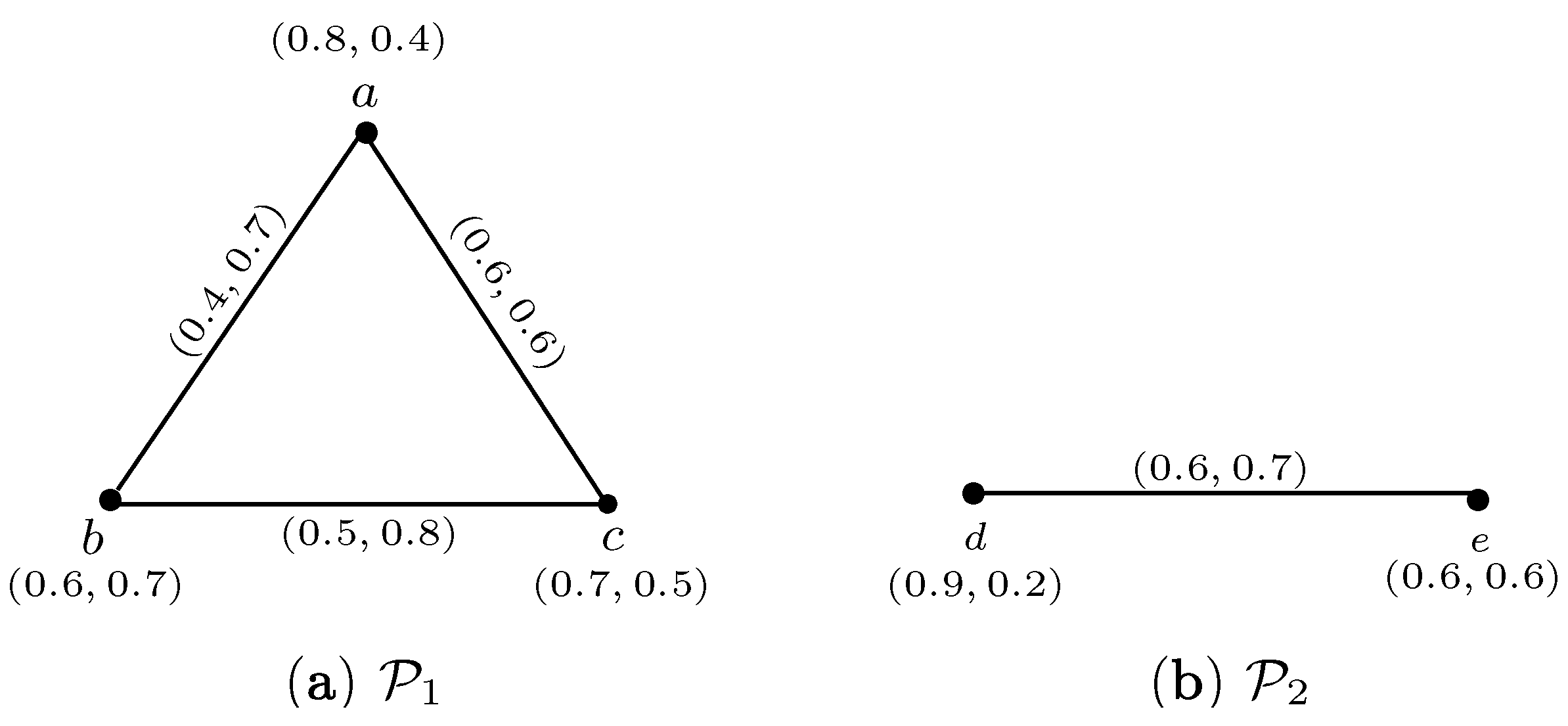
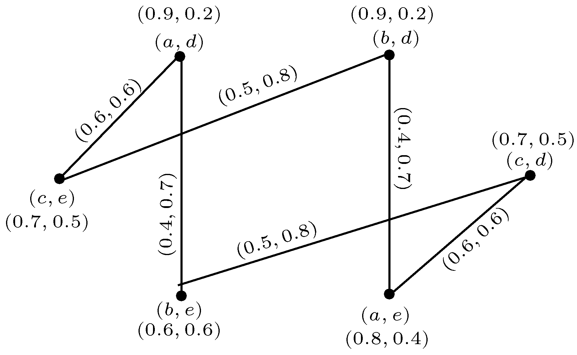
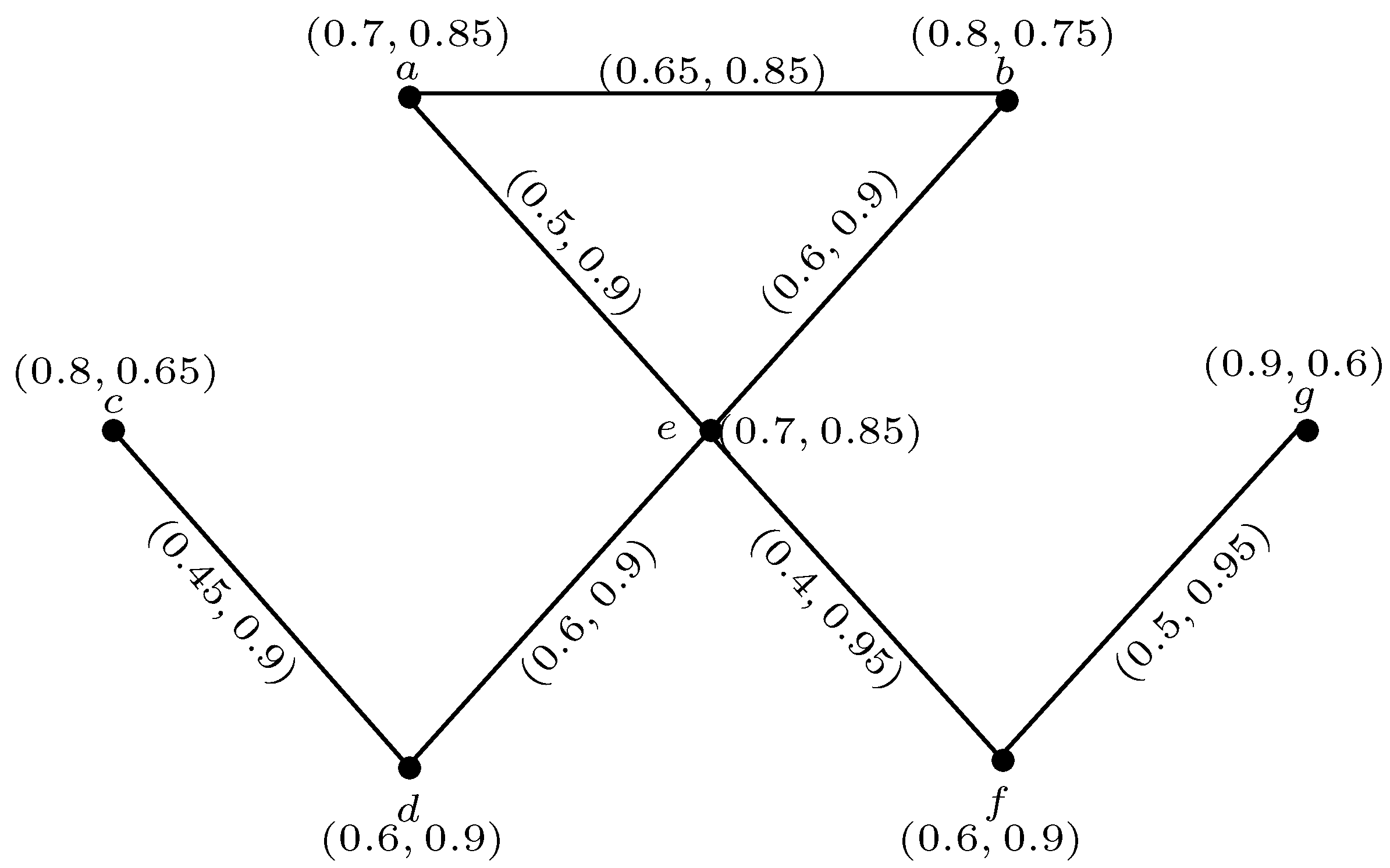
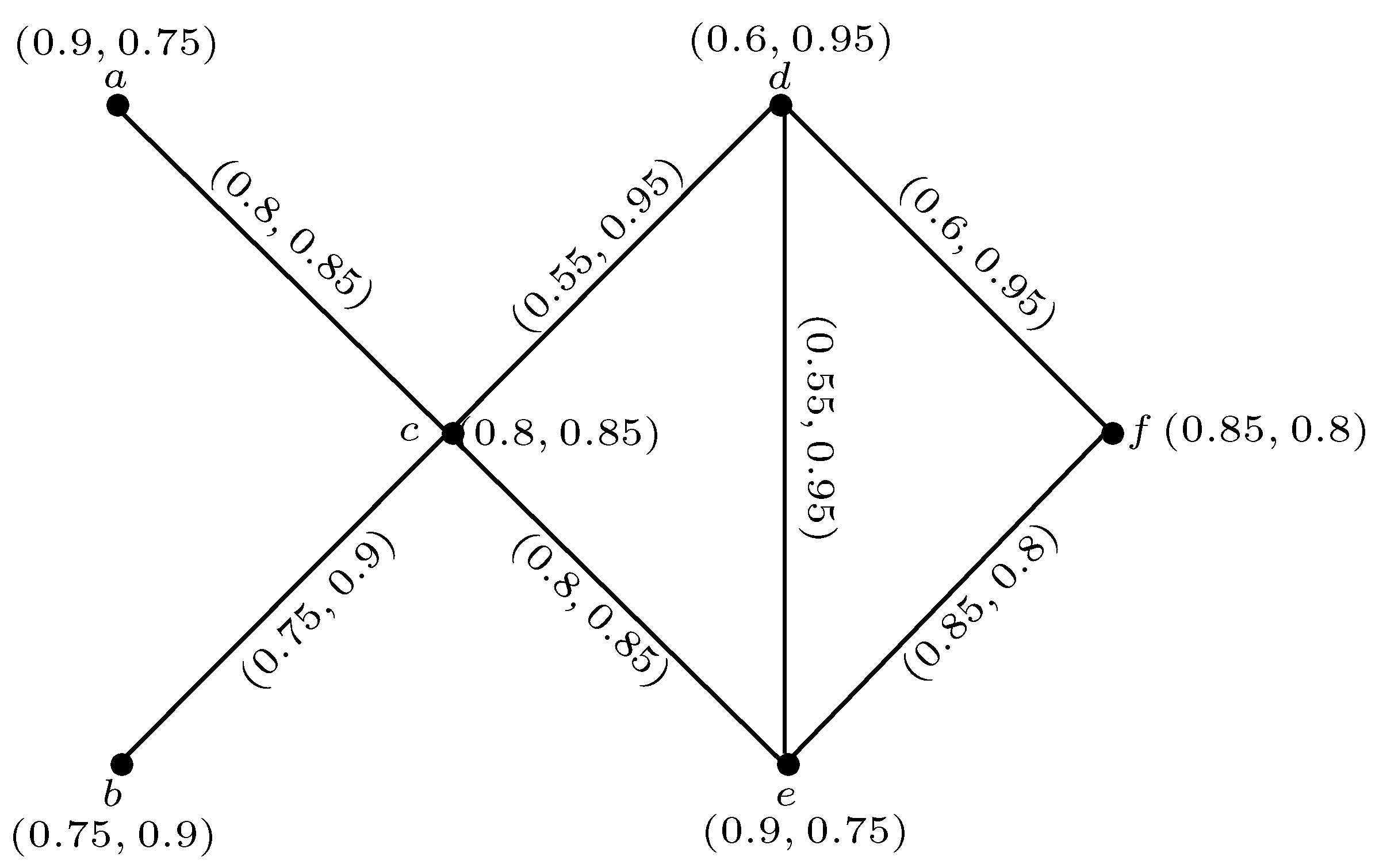
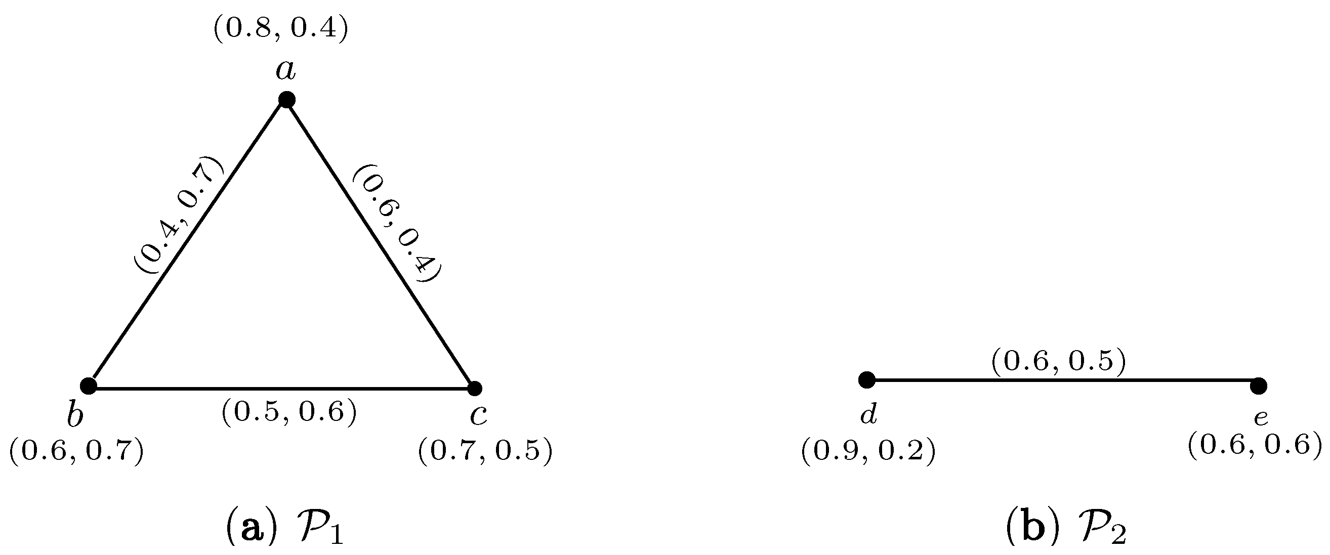
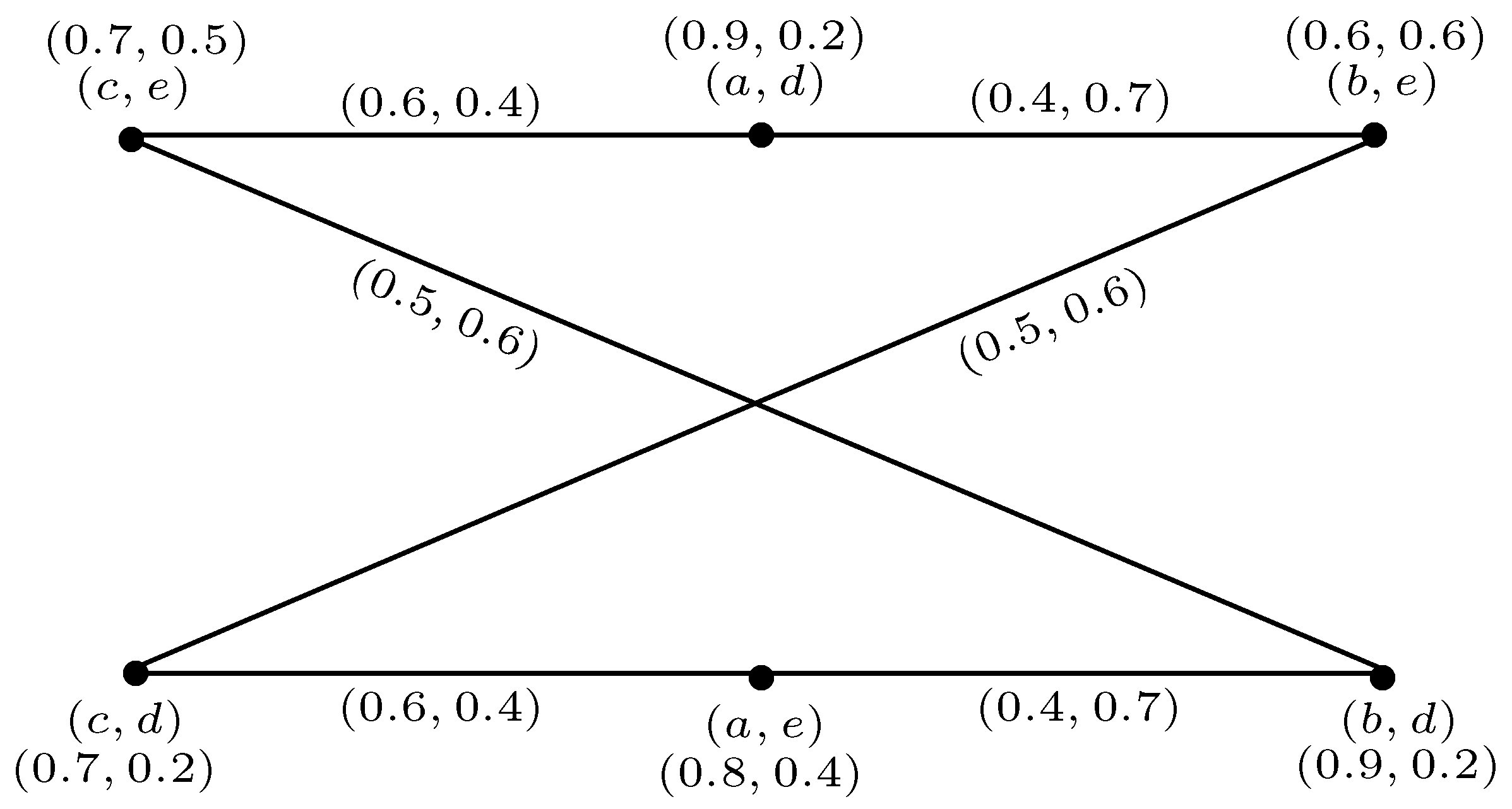
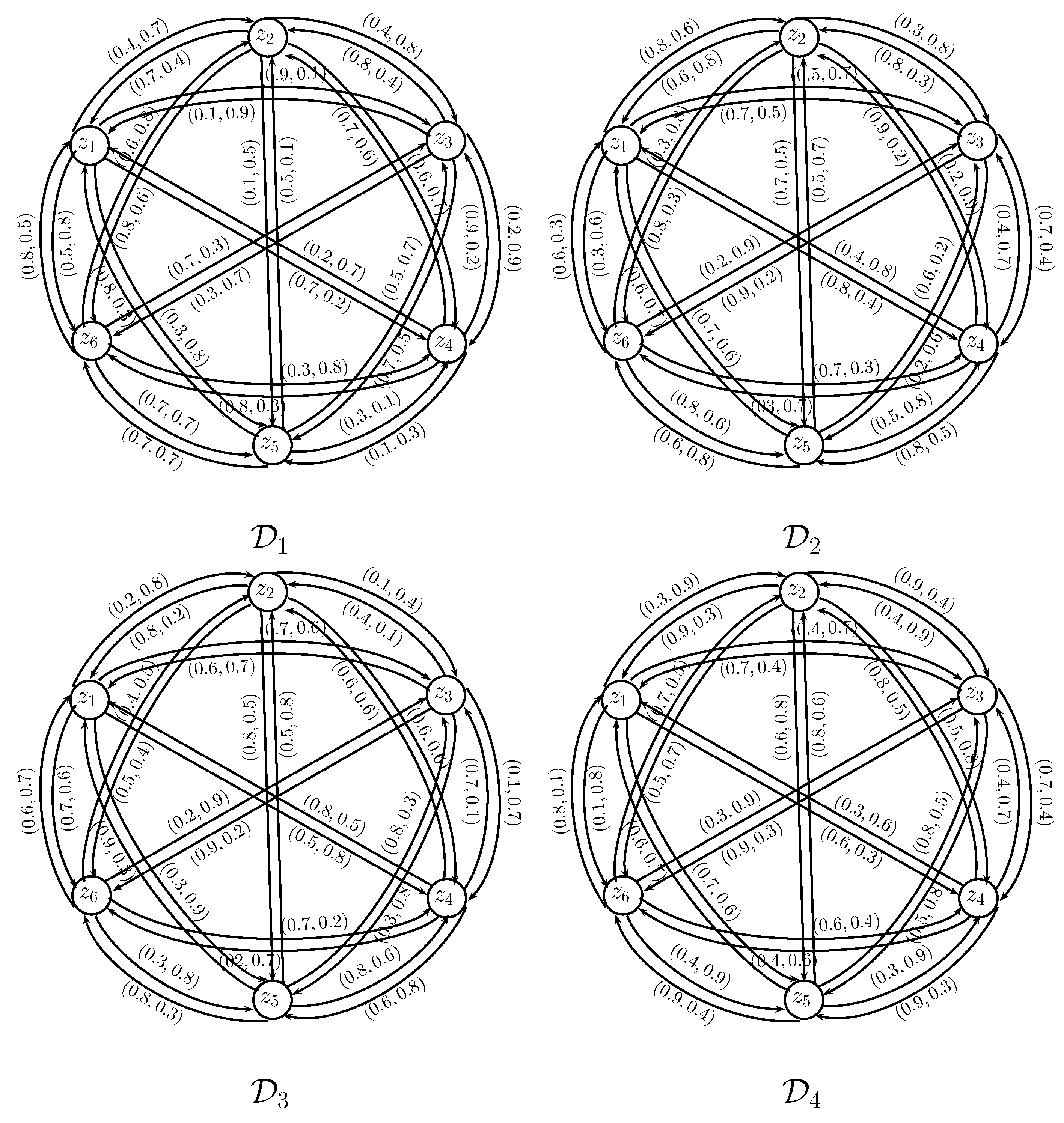
Example 4.

Consider two PFGs ${\mathcal{P}}_1=({\mathcal{C}}_1,{\mathcal{D}}_1)and{\mathcal{P}}_2=({\mathcal{C}}_2,{\mathcal{D}}_2)on{V}_1=\{a,b\}and{V}_2=\{c,d,e\}$, respectively, as shown in Figure 5. Their symmetric difference ${\mathcal{P}}_1\oplus {\mathcal{P}}_2$ is shown in Figure 6.

Proposition 2.

Let ${\mathcal{P}}_{1}and{\mathcal{P}}_2$ be two PFGs of the graphs $G_{1}and{G}_2$, respectively. The symmetric difference ${\mathcal{P}}_1\oplus {\mathcal{P}}_2$ of ${\mathcal{P}}_{1}and{\mathcal{P}}_2$ is a PFG of $G_1\oplus G_2$.

Proof. 

Let ${\mathcal{P}}_1=({\mathcal{C}}_1,{\mathcal{D}}_1)and{\mathcal{P}}_2=({\mathcal{C}}_2,{\mathcal{D}}_2)$ be two PFGs of the graphs $G_{1}and{G}_2$, respectively. Let $(x_1,x_2)(y_1,y_2)\in E_1\times E_2.$

If $x_1=y_1=x$,

$$\begin{array}{ccc}\hfill ({\mu }_{{\mathcal{D}}_1}\oplus {\mu }_{{\mathcal{D}}_2})\left((x,x_2)(x,y_2)\right)& =& {\mu }_{{\mathcal{C}}_1}\left(x\right)\wedge {\mu }_{{\mathcal{D}}_2}\left(x_2{y}_2\right)\hfill \\ & \le & {\mu }_{{\mathcal{C}}_1}\left(x\right)\wedge \{{\mu }_{{\mathcal{C}}_2}\left(x_2\right)\wedge {\mu }_{{\mathcal{C}}_2}\left(y_2\right)\}\hfill \\ & =& \{{\mu }_{{\mathcal{C}}_1}\left(x\right)\wedge {\mu }_{{\mathcal{C}}_2}\left(x_2\right)\}\wedge \{{\mu }_{{\mathcal{C}}_1}\left(x\right)\wedge {\mu }_{{\mathcal{C}}_2}\left(y_2\right)\}\hfill \\ & =& ({\mu }_{{\mathcal{C}}_1}\oplus {\mu }_{{\mathcal{C}}_2})(x,x_2)\wedge ({\mu }_{{\mathcal{C}}_1}\oplus {\mu }_{{\mathcal{C}}_2})(x,y_2),\hfill \end{array}$$

$$\begin{array}{ccc}\hfill ({\nu }_{{\mathcal{D}}_1}\oplus {\nu }_{{\mathcal{D}}_2})\left((x,x_2)(x,y_2)\right)& =& {\nu }_{{\mathcal{C}}_1}\left(x\right)\vee {\nu }_{{\mathcal{D}}_2}\left(x_2{y}_2\right)\hfill \\ & \ge & {\nu }_{{\mathcal{C}}_1}\left(x\right)\vee \{{\nu }_{{\mathcal{C}}_2}\left(x_2\right)\vee {\nu }_{{\mathcal{C}}_2}\left(y_2\right)\}\hfill \\ & =& \{{\nu }_{{\mathcal{C}}_1}\left(x\right)\vee {\nu }_{{\mathcal{C}}_2}\left(x_2\right)\}\vee \{{\nu }_{{\mathcal{C}}_1}\left(x\right)\vee {\nu }_{{\mathcal{C}}_2}\left(y_2\right)\}\hfill \\ & =& ({\nu }_{{\mathcal{C}}_1}\oplus {\nu }_{{\mathcal{C}}_2})(x,x_2)\vee ({\nu }_{{\mathcal{C}}_1}\oplus {\nu }_{{\mathcal{C}}_2})(x,y_2).\hfill \end{array}$$

If $x_2=y_2=z$,

$$\begin{array}{ccc}\hfill ({\mu }_{{\mathcal{D}}_1}\oplus {\mu }_{{\mathcal{D}}_2})\left((x_1,z)(y_1,z)\right)& =& {\mu }_{{\mathcal{D}}_1}\left(x_1{y}_1\right)\wedge {\mu }_{{\mathcal{C}}_2}\left(z\right)\hfill \\ & \le & \{{\mu }_{{\mathcal{C}}_1}\left(x_1\right)\wedge {\mu }_{{\mathcal{C}}_1}\left(y_1\right)\}\wedge {\mu }_{{\mathcal{C}}_2}\left(z\right)\hfill \\ & =& \{{\mu }_{{\mathcal{C}}_1}\left(x_1\right)\wedge {\mu }_{{\mathcal{C}}_2}\left(z\right)\}\wedge \{{\mu }_{{\mathcal{C}}_1}\left(y_1\right)\wedge {\mu }_{{\mathcal{C}}_2}\left(z\right)\}\hfill \\ & =& ({\mu }_{{\mathcal{C}}_1}\oplus {\mu }_{{\mathcal{C}}_2})(x_1,z)\wedge ({\mu }_{{\mathcal{C}}_1}\oplus {\mu }_{{\mathcal{C}}_2})(y_1,z),\hfill \end{array}$$

$$\begin{array}{ccc}\hfill ({\nu }_{{\mathcal{D}}_1}\oplus {\nu }_{{\mathcal{D}}_2})\left((x_1,z)(y_1,z)\right)& =& {\nu }_{{\mathcal{D}}_1}\left(x_1{y}_1\right)\vee {\nu }_{{\mathcal{C}}_2}\left(z\right)\hfill \\ & \ge & \{{\nu }_{{\mathcal{C}}_1}\left(x_1\right)\vee {\nu }_{{\mathcal{C}}_1}\left(y_1\right)\}\vee {\nu }_{{\mathcal{C}}_2}\left(z\right)\hfill \\ & =& \{{\nu }_{{\mathcal{C}}_1}\left(x_1\right)\vee {\nu }_{{\mathcal{C}}_2}\left(z\right)\}\vee \{{\nu }_{{\mathcal{C}}_1}\left(y_1\right)\vee {\nu }_{{\mathcal{C}}_2}\left(z\right)\}\hfill \\ & =& ({\nu }_{{\mathcal{C}}_1}\oplus {\nu }_{{\mathcal{C}}_2})(x_1,z)\vee ({\nu }_{{\mathcal{C}}_1}\oplus {\nu }_{{\mathcal{C}}_2})(y_1,z).\hfill \end{array}$$

If $x_1{y}_1\notin E_1\mathrm{and}{x}_2{y}_2\in E_2$,

$$\begin{array}{ccc}\hfill ({\mu }_{{\mathcal{D}}_1}\oplus {\mu }_{{\mathcal{D}}_2})\left((x_1,x_2)(y_1,y_2)\right)& =& {\mu }_{{\mathcal{C}}_1}\left(x_1\right)\wedge {\mu }_{{\mathcal{C}}_1}\left(y_1\right)\wedge {\mu }_{{\mathcal{D}}_2}\left(x_2{y}_2\right)\hfill \\ & \le & {\mu }_{{\mathcal{C}}_1}\left(x_1\right)\wedge {\mu }_{{\mathcal{C}}_1}\left(y_1\right)\wedge \{{\mu }_{{\mathcal{C}}_2}\left(x_2\right)\wedge {\mu }_{{\mathcal{C}}_2}\left(y_2\right)\}\hfill \\ & =& \{{\mu }_{{\mathcal{C}}_1}\left(x_1\right)\wedge {\mu }_{{\mathcal{C}}_2}\left(x_2\right)\}\wedge \{{\mu }_{{\mathcal{C}}_1}\left(y_1\right)\wedge {\mu }_{{\mathcal{C}}_2}\left(y_2\right)\}\hfill \\ & =& ({\mu }_{{\mathcal{C}}_1}\oplus {\mu }_{{\mathcal{C}}_2})(x_1,x_2)\wedge ({\mu }_{{\mathcal{C}}_1}\oplus {\mu }_{{\mathcal{C}}_2})(y_1,y_2),\hfill \end{array}$$

$$\begin{array}{ccc}\hfill ({\nu }_{{\mathcal{D}}_1}\oplus {\nu }_{{\mathcal{D}}_2})\left((x_1,x_2)(y_1,y_2)\right)& =& {\nu }_{{\mathcal{C}}_1}\left(x_1\right)\vee {\nu }_{{\mathcal{C}}_1}\left(y_1\right)\vee {\nu }_{{\mathcal{D}}_2}\left(x_2{y}_2\right)\hfill \\ & \ge & {\nu }_{{\mathcal{C}}_1}\left(x_1\right)\vee {\nu }_{{\mathcal{C}}_1}\left(y_1\right)\vee \{{\nu }_{{\mathcal{C}}_2}\left(x_2\right)\vee {\nu }_{{\mathcal{C}}_2}\left(y_2\right)\}\hfill \\ & =& \{{\nu }_{{\mathcal{C}}_1}\left(x_1\right)\vee {\nu }_{{\mathcal{C}}_2}\left(x_2\right)\}\vee \{{\nu }_{{\mathcal{C}}_1}\left(y_1\right)\vee {\nu }_{{\mathcal{C}}_2}\left(y_2\right)\}\hfill \\ & =& ({\nu }_{{\mathcal{C}}_1}\oplus {\nu }_{{\mathcal{C}}_2})(x_1,x_2)\vee ({\nu }_{{\mathcal{C}}_1}\oplus {\nu }_{{\mathcal{C}}_2})(y_1,y_2).\hfill \end{array}$$

If $x_1{y}_1\in E_1\mathrm{and}{x}_2{y}_2\notin E_2$,

$$\begin{array}{ccc}\hfill ({\mu }_{{\mathcal{D}}_1}\oplus {\mu }_{{\mathcal{D}}_2})\left((x_1,x_2)(y_1,y_2)\right)& =& {\mu }_{{\mathcal{D}}_1}\left(x_1{y}_1\right)\wedge {\mu }_{{\mathcal{C}}_2}\left(x_2\right)\wedge {\mu }_{{\mathcal{C}}_2}\left(y_2\right)\hfill \\ & \le & \{{\mu }_{{\mathcal{C}}_1}\left(x_1\right)\wedge {\mu }_{{\mathcal{C}}_1}\left(y_1\right)\}\wedge {\mu }_{{\mathcal{C}}_2}\left(x_2\right)\wedge {\mu }_{{\mathcal{C}}_2}\left(y_2\right)\hfill \\ & =& \{{\mu }_{{\mathcal{C}}_1}\left(x_1\right)\wedge {\mu }_{{\mathcal{C}}_2}\left(x_2\right)\}\wedge \{{\mu }_{{\mathcal{C}}_1}\left(y_1\right)\wedge {\mu }_{{\mathcal{C}}_2}\left(y_2\right)\}\hfill \\ & =& ({\mu }_{{\mathcal{C}}_1}\oplus {\mu }_{{\mathcal{C}}_2})(x_1,x_2)\wedge ({\mu }_{{\mathcal{C}}_1}\oplus {\mu }_{{\mathcal{C}}_2})(y_1,y_2),\hfill \end{array}$$

$$\begin{array}{ccc}\hfill ({\nu }_{{\mathcal{D}}_1}\oplus {\nu }_{{\mathcal{D}}_2})\left((x_1,x_2)(y_1,y_2)\right)& =& {\nu }_{{\mathcal{D}}_1}\left(x_1{y}_1\right)\vee {\nu }_{{\mathcal{C}}_2}\left(x_2\right)\vee {\nu }_{{\mathcal{C}}_2}\left(y_2\right)\hfill \\ & \ge & \{{\nu }_{{\mathcal{C}}_1}\left(x_1\right)\vee {\nu }_{{\mathcal{C}}_1}\left(y_1\right)\}\vee {\nu }_{{\mathcal{C}}_2}\left(x_2\right)\vee {\nu }_{{\mathcal{C}}_2}\left(y_2\right)\hfill \\ & =& \{{\nu }_{{\mathcal{C}}_1}\left(x_1\right)\vee {\nu }_{{\mathcal{C}}_2}\left(x_2\right)\}\vee \{{\nu }_{{\mathcal{C}}_1}\left(y_1\right)\vee {\nu }_{{\mathcal{C}}_2}\left(y_2\right)\}\hfill \\ & =& ({\nu }_{{\mathcal{C}}_1}\oplus {\nu }_{{\mathcal{C}}_2})(x_1,x_2)\vee ({\nu }_{{\mathcal{C}}_1}\oplus {\nu }_{{\mathcal{C}}_2})(y_1,y_2).\hfill \end{array}$$

Hence, ${\mathcal{P}}_1\oplus {\mathcal{P}}_2$ is a PFG. ☐

Definition 6.

Let ${\mathcal{P}}_1=({\mathcal{C}}_1,{\mathcal{D}}_1)and{\mathcal{P}}_2=({\mathcal{C}}_2,{\mathcal{D}}_2)$ be two PFGs. For any vertex $(x_1,x_2)\in V_1\times V_2$,

$$\begin{array}{c}\hfill \begin{array}{cc}\hfill {\left(d_{\mu }\right)}_{{\mathcal{P}}_1\oplus {\mathcal{P}}_2}(x_1,x_2)& =\sum _{(x_1,x_2)(y_1,y_2)\in E_1\times E_2}({\mu }_{{\mathcal{D}}_1}\oplus {\mu }_{{\mathcal{D}}_1})\left((x_1,x_2)(y_1,y_2)\right)\hfill \\ & =\sum _{x_1=y_1,x_2{y}_2\in E_2}{\mu }_{{\mathcal{C}}_1}\left(x_1\right)\wedge {\mu }_{{\mathcal{D}}_2}\left(x_2{y}_2\right)+\sum _{x_1{y}_1\in E_1,x_2=y_2}{\mu }_{{\mathcal{D}}_1}\left(x_1{y}_1\right)\wedge {\mu }_{{\mathcal{C}}_2}\left(x_2\right)\hfill \\ & +\sum _{x_1{y}_1\notin E_1,x_2{y}_2\in E_2}{\mu }_{{\mathcal{C}}_1}\left(x_1\right)\wedge {\mu }_{{\mathcal{C}}_1}\left(y_1\right)\wedge {\mu }_{{\mathcal{D}}_2}\left(x_2{y}_2\right)\hfill \\ & +\sum _{x_1{y}_1\in E_1,x_2{y}_2\notin E_2}{\mu }_{{\mathcal{D}}_1}\left(x_1{y}_1\right)\wedge {\mu }_{{\mathcal{C}}_2}\left(x_2\right)\wedge {\mu }_{{\mathcal{C}}_2}\left(y_2\right),\hfill \end{array}\end{array}$$

$$\begin{array}{c}\hfill \begin{array}{cc}\hfill {\left(d_{\nu }\right)}_{{\mathcal{P}}_1\oplus {\mathcal{P}}_2}(x_1,x_2)& =\sum _{(x_1,x_2)(y_1,y_2)\in E_1\times E_2}({\nu }_{{\mathcal{D}}_1}\oplus {\nu }_{{\mathcal{D}}_1})\left((x_1,x_2)(y_1,y_2)\right)\hfill \\ & =\sum _{x_1=y_1,x_2{y}_2\in E_2}{\nu }_{{\mathcal{C}}_1}\left(x_1\right)\vee {\nu }_{{\mathcal{D}}_2}\left(x_2{y}_2\right)+\sum _{x_1{y}_1\in E_1,x_2=y_2}{\nu }_{{\mathcal{D}}_1}\left(x_1{y}_1\right)\vee {\nu }_{{\mathcal{C}}_2}\left(x_2\right)\hfill \\ & +\sum _{x_1{y}_1\notin E_1,x_2{y}_2\in E_2}{\nu }_{{\mathcal{C}}_1}\left(x_1\right)\vee {\nu }_{{\mathcal{C}}_1}\left(y_1\right)\vee {\nu }_{{\mathcal{D}}_2}\left(x_2{y}_2\right)\hfill \\ & +\sum _{x_1{y}_1\in E_1,x_2{y}_2\notin E_2}{\nu }_{{\mathcal{D}}_1}\left(x_1{y}_1\right)\vee {\nu }_{{\mathcal{C}}_2}\left(x_2\right)\vee {\nu }_{{\mathcal{C}}_2}\left(y_2\right).\hfill \end{array}\end{array}$$

Theorem 1.

Let ${\mathcal{P}}_{1}and{\mathcal{P}}_2$ be two PFGs. If ${\mu }_{{\mathcal{C}}_1}\ge {\mu }_{{\mathcal{D}}_2},{\nu }_{{\mathcal{C}}_1}\le {\nu }_{{\mathcal{D}}_2}and{\mu }_{{\mathcal{C}}_2}\ge {\mu }_{{\mathcal{D}}_1},{\nu }_{{\mathcal{C}}_2}\le {\nu }_{{\mathcal{D}}_1}$. Then, for all $(x_1,x_2)\in V_1\times V_2,d_{{\mathcal{P}}_1\oplus {\mathcal{P}}_2}(x_1,x_2)={\mathit{p}}_{\mathit{2}}{d}_{{\mathcal{P}}_1}\left(x_1\right)+{\mathit{p}}_{\mathit{1}}{d}_{{\mathcal{P}}_2}\left(x_2\right)$, where ${\mathit{p}}_{\mathit{1}}=\mid {\mathit{V}}_{\mathit{1}}\mid -{\mathit{d}}_{{\mathit{G}}_{\mathit{1}}}\left({\mathit{x}}_{\mathit{1}}\right)\mathit{and}{\mathit{p}}_{\mathit{2}}=\mid {\mathit{V}}_{\mathit{2}}\mid -{\mathit{d}}_{{\mathit{G}}_{\mathit{2}}}\left({\mathit{x}}_{\mathit{2}}\right)$.

Proof. 

By definition of vertex degree of symmetric difference, we have

$$\begin{array}{c}\hfill \begin{array}{cc}\hfill {\left(d_{\mu }\right)}_{{\mathcal{P}}_1\oplus {\mathcal{P}}_2}(x_1,x_2)& =\sum _{(x_1,x_2)(y_1,y_2)\in E_1\times E_2}({\mu }_{{\mathcal{D}}_1}\oplus {\mu }_{{\mathcal{D}}_1})\left((x_1,x_2)(y_1,y_2)\right)\hfill \\ & =\sum _{x_1=y_1,x_2{y}_2\in E_2}{\mu }_{{\mathcal{C}}_1}\left(x_1\right)\wedge {\mu }_{{\mathcal{D}}_2}\left(x_2{y}_2\right)+\sum _{x_1{y}_1\in E_1,x_2=y_2}{\mu }_{{\mathcal{D}}_1}\left(x_1{y}_1\right)\wedge {\mu }_{{\mathcal{C}}_2}\left(x_2\right)\hfill \\ & +\sum _{x_1{y}_1\notin E_1,x_2{y}_2\in E_2}{\mu }_{{\mathcal{C}}_1}\left(x_1\right)\wedge {\mu }_{{\mathcal{C}}_1}\left(y_1\right)\wedge {\mu }_{{\mathcal{D}}_2}\left(x_2{y}_2\right)\hfill \\ & +\sum _{x_1{y}_1\in E_1,x_2{y}_2\notin E_2}{\mu }_{{\mathcal{D}}_1}\left(x_1{y}_1\right)\wedge {\mu }_{{\mathcal{C}}_2}\left(x_2\right)\wedge {\mu }_{{\mathcal{C}}_2}\left(y_2\right)\hfill \\ & =\sum _{x_2{y}_2\in E_2}{\mu }_{{\mathcal{D}}_2}\left(x_2{y}_2\right)+\sum _{x_1{y}_1\in E_1}{\mu }_{{\mathcal{D}}_1}\left(x_1{y}_1\right)+\sum _{x_1{y}_1\notin E_1,x_2{y}_2\in E_2}{\mu }_{{\mathcal{D}}_2}\left(x_2{y}_2\right)\hfill \\ & +\sum _{x_1{y}_1\in E_1,x_2{y}_2\notin E_2}{\mu }_{{\mathcal{D}}_1}\left(x_1{y}_1\right)\hfill \\ & ={\mathit{p}}_{\mathit{2}}{\left(d_{\mu }\right)}_{{\mathcal{P}}_1}\left(x_1\right)+{\mathit{p}}_{\mathit{1}}{\left(d_{\mu }\right)}_{{\mathcal{P}}_2}\left(x_2\right),\hfill \end{array}\end{array}$$

$$\begin{array}{c}\hfill \begin{array}{cc}\hfill {\left(d_{\nu }\right)}_{{\mathcal{P}}_1\oplus {\mathcal{P}}_2}(x_1,x_2)& =\sum _{(x_1,x_2)(y_1,y_2)\in E_1\times E_2}({\nu }_{{\mathcal{D}}_1}\oplus {\nu }_{{\mathcal{D}}_1})\left((x_1,x_2)(y_1,y_2)\right)\hfill \\ & =\sum _{x_1=y_1,x_2{y}_2\in E_2}{\nu }_{{\mathcal{C}}_1}\left(x_1\right)\vee {\nu }_{{\mathcal{D}}_2}\left(x_2{y}_2\right)+\sum _{x_1{y}_1\in E_1,x_2=y_2}{\nu }_{{\mathcal{D}}_1}\left(x_1{y}_1\right)\vee {\nu }_{{\mathcal{C}}_2}\left(x_2\right)\hfill \\ & +\sum _{x_1{y}_1\notin E_1,x_2{y}_2\in E_2}{\nu }_{{\mathcal{C}}_1}\left(x_1\right)\vee {\nu }_{{\mathcal{C}}_1}\left(y_1\right)\vee {\nu }_{{\mathcal{D}}_2}\left(x_2{y}_2\right)\hfill \\ & +\sum _{x_1{y}_1\in E_1,x_2{y}_2\notin E_2}{\nu }_{{\mathcal{D}}_1}\left(x_1{y}_1\right)\vee {\nu }_{{\mathcal{C}}_2}\left(x_2\right)\vee {\nu }_{{\mathcal{C}}_2}\left(y_2\right)\hfill \\ & =\sum _{x_2{y}_2\in E_2}{\nu }_{{\mathcal{D}}_2}\left(x_2{y}_2\right)+\sum _{x_1{y}_1\in E_1}{\nu }_{{\mathcal{D}}_1}\left(x_1{y}_1\right)+\sum _{x_1{y}_1\notin E_1,x_2{y}_2\in E_2}{\nu }_{{\mathcal{D}}_2}\left(x_2{y}_2\right)\hfill \\ & +\sum _{x_1{y}_1\in E_1,x_2{y}_2\notin E_2}{\nu }_{{\mathcal{D}}_1}\left(x_1{y}_1\right)\hfill \\ & ={\mathit{p}}_{\mathit{2}}{\left(d_{\nu }\right)}_{{\mathcal{P}}_1}\left(x_1\right)+{\mathit{p}}_{\mathit{1}}{\left(d_{\nu }\right)}_{{\mathcal{P}}_2}\left(x_2\right).\hfill \end{array}\end{array}$$

Hence,$d_{{\mathcal{P}}_1\oplus {\mathcal{P}}_2}(x_1,x_2)={\mathit{p}}_{\mathit{2}}{d}_{{\mathcal{P}}_1}\left(x_1\right)+{\mathit{p}}_{\mathit{1}}{d}_{{\mathcal{P}}_2}\left(x_2\right)$, where ${\mathit{p}}_{\mathit{1}}=\mid {\mathit{V}}_{\mathit{1}}\mid -{\mathit{d}}_{{\mathit{G}}_{\mathit{1}}}\left({\mathit{x}}_{\mathit{1}}\right)\mathrm{and}{\mathit{p}}_{\mathit{2}}=\mid {\mathit{V}}_{\mathit{2}}\mid -{\mathit{d}}_{{\mathit{G}}_{\mathit{2}}}\left({\mathit{x}}_{\mathit{2}}\right)$. ☐

Definition 7.

Let ${\mathcal{P}}_1=({\mathcal{C}}_1,{\mathcal{D}}_1)and{\mathcal{P}}_2=({\mathcal{C}}_2,{\mathcal{D}}_2)$ be two PFGs. For any vertex $(x_1,x_2)\in V_1\times V_2$,

$$\begin{array}{c}\hfill \begin{array}{cc}\hfill {\left(t{d}_{\mu }\right)}_{{\mathcal{P}}_1\oplus {\mathcal{P}}_2}(x_1,x_2)& =\sum _{(x_1,x_2)(y_1,y_2)\in E_1\times E_2}({\mu }_{{\mathcal{D}}_1}\oplus {\mu }_{{\mathcal{D}}_1})\left((x_1,x_2)(y_1,y_2)\right)+({\mu }_{{\mathcal{C}}_1}\oplus {\mu }_{{\mathcal{C}}_2})(x_1,x_2)\hfill \\ & =\sum _{x_1=y_1,x_2{y}_2\in E_2}{\mu }_{{\mathcal{C}}_1}\left(x_1\right)\wedge {\mu }_{{\mathcal{D}}_2}\left(x_2{y}_2\right)+\sum _{x_1{y}_1\in E_1,x_2=y_2}{\mu }_{{\mathcal{D}}_1}\left(x_1{y}_1\right)\wedge {\mu }_{{\mathcal{C}}_2}\left(x_2\right)\hfill \\ & +\sum _{x_1{y}_1\notin E_1,x_2{y}_2\in E_2}{\mu }_{{\mathcal{C}}_1}\left(x_1\right)\wedge {\mu }_{{\mathcal{C}}_1}\left(y_1\right)\wedge {\mu }_{{\mathcal{D}}_2}\left(x_2{y}_2\right)\hfill \\ & +\sum _{x_1{y}_1\in E_1,x_2{y}_2\notin E_2}{\mu }_{{\mathcal{D}}_1}\left(x_1{y}_1\right)\wedge {\mu }_{{\mathcal{C}}_2}\left(x_2\right)\wedge {\mu }_{{\mathcal{C}}_2}\left(y_2\right)+{\mu }_{{\mathcal{C}}_1}\left(x_1\right)\wedge {\mu }_{{\mathcal{C}}_2}\left(x_2\right),\hfill \end{array}\end{array}$$

$$\begin{array}{c}\hfill \begin{array}{cc}\hfill {\left(d_{\nu }\right)}_{{\mathcal{P}}_1\oplus {\mathcal{P}}_2}(x_1,x_2)& =\sum _{(x_1,x_2)(y_1,y_2)\in E_1\times E_2}({\nu }_{{\mathcal{D}}_1}\oplus {\nu }_{{\mathcal{D}}_1})\left((x_1,x_2)(y_1,y_2)\right)+({\nu }_{{\mathcal{C}}_1}\oplus {\nu }_{{\mathcal{C}}_2})(x_1,x_2)\hfill \\ & =\sum _{x_1=y_1,x_2{y}_2\in E_2}{\nu }_{{\mathcal{C}}_1}\left(x_1\right)\vee {\nu }_{{\mathcal{D}}_2}\left(x_2{y}_2\right)+\sum _{x_1{y}_1\in E_1,x_2=y_2}{\nu }_{{\mathcal{D}}_1}\left(x_1{y}_1\right)\vee {\nu }_{{\mathcal{C}}_2}\left(x_2\right)\hfill \\ & +\sum _{x_1{y}_1\notin E_1,x_2{y}_2\in E_2}{\nu }_{{\mathcal{C}}_1}\left(x_1\right)\vee {\nu }_{{\mathcal{C}}_1}\left(y_1\right)\vee {\nu }_{{\mathcal{D}}_2}\left(x_2{y}_2\right)\hfill \\ & +\sum _{x_1{y}_1\in E_1,x_2{y}_2\notin E_2}{\nu }_{{\mathcal{D}}_1}\left(x_1{y}_1\right)\vee {\nu }_{{\mathcal{C}}_2}\left(x_2\right)\vee {\nu }_{{\mathcal{C}}_2}\left(y_2\right)+{\nu }_{{\mathcal{C}}_1}\left(x_1\right)\vee {\nu }_{{\mathcal{C}}_2}\left(x_2\right).\hfill \end{array}\end{array}$$

Theorem 2.

Let ${\mathcal{P}}_1=({\mathcal{C}}_1,{\mathcal{D}}_1)and{\mathcal{P}}_2=({\mathcal{C}}_2,{\mathcal{D}}_2)$ be two PFGs. If

(i)

${\mu }_{{\mathcal{C}}_1}\ge {\mu }_{{\mathcal{D}}_2}and{\mu }_{{\mathcal{C}}_2}\ge {\mu }_{{\mathcal{D}}_1},then$

$${\left(t{d}_{\mu }\right)}_{{\mathcal{P}}_1\oplus {\mathcal{P}}_2}(x_1,x_2)={\mathit{p}}_{\mathit{2}}{\left(t{d}_{\mu }\right)}_{{\mathcal{P}}_1}\left(x_1\right)+{\mathit{p}}_{\mathit{1}}{\left(t{d}_{\mu }\right)}_{{\mathcal{P}}_2}\left(x_2\right)-({\mathit{p}}_{\mathit{1}}-\mathit{1}){\mu }_{p_2}\left(x_2\right)-({\mathit{p}}_{\mathit{2}}-\mathit{1}){\mu }_{p_1}\left(x_1\right)-{\mu }_{p_1}\left(x_1\right)\vee {\mu }_{p_2}\left(x_2\right)$$

(ii)

${\nu }_{{\mathcal{C}}_1}\le {\nu }_{{\mathcal{D}}_2}and{\nu }_{{\mathcal{C}}_2}\le {\nu }_{{\mathcal{D}}_1},then$

$${\left(t{d}_{\nu }\right)}_{{\mathcal{P}}_1\oplus {\mathcal{P}}_2}(x_1,x_2)={\mathit{p}}_{\mathit{2}}{\left(t{d}_{\nu }\right)}_{{\mathcal{P}}_1}\left(x_1\right)+{\mathit{p}}_{\mathit{1}}{\left(t{d}_{\nu }\right)}_{{\mathcal{P}}_2}\left(x_2\right)-({\mathit{p}}_{\mathit{1}}-\mathit{1}){\nu }_{p_2}\left(x_2\right)-({\mathit{p}}_{\mathit{2}}-\mathit{1}){\nu }_{p_1}\left(x_1\right)-{\nu }_{p_1}\left(x_1\right)\wedge {\nu }_{p_2}\left(x_2\right)$$

for all $(x_1,x_2)\in V_1\times V_2,{\mathit{p}}_{\mathit{1}}=\mid {\mathit{V}}_{\mathit{1}}\mid -{\mathit{d}}_{{\mathit{G}}_{\mathit{1}}}\left({\mathit{x}}_{\mathit{1}}\right)\mathit{and}{\mathit{p}}_{\mathit{2}}=\mid {\mathit{V}}_{\mathit{2}}\mid -{\mathit{d}}_{{\mathit{G}}_{\mathit{2}}}\left({\mathit{x}}_{\mathit{2}}\right).$

Proof. 

For any vertex $(x_1,x_2)\in V_1\times V_2$,

$$\begin{array}{c}\hfill \begin{array}{cc}\hfill {\left(t{d}_{\mu }\right)}_{{\mathcal{P}}_1\oplus {\mathcal{P}}_2}(x_1,x_2)& =\sum _{(x_1,x_2)(y_1,y_2)\in E_1\times E_2}({\mu }_{{\mathcal{D}}_1}\oplus {\mu }_{{\mathcal{D}}_1})\left((x_1,x_2)(y_1,y_2)\right)\hfill \\ & =\sum _{x_1=y_1,x_2{y}_2\in E_2}{\mu }_{{\mathcal{C}}_1}\left(x_1\right)\wedge {\mu }_{{\mathcal{D}}_2}\left(x_2{y}_2\right)+\sum _{x_1{y}_1\in E_1,x_2=y_2}{\mu }_{{\mathcal{D}}_1}\left(x_1{y}_1\right)\wedge {\mu }_{{\mathcal{C}}_2}\left(x_2\right)\hfill \\ & +\sum _{x_1{y}_1\notin E_1,x_2{y}_2\in E_2}{\mu }_{{\mathcal{C}}_1}\left(x_1\right)\wedge {\mu }_{{\mathcal{C}}_1}\left(y_1\right)\wedge {\mu }_{{\mathcal{D}}_2}\left(x_2{y}_2\right)\hfill \\ & +\sum _{x_1{y}_1\in E_1,x_2{y}_2\notin E_2}{\mu }_{{\mathcal{D}}_1}\left(x_1{y}_1\right)\wedge {\mu }_{{\mathcal{C}}_2}\left(x_2\right)\wedge {\mu }_{{\mathcal{C}}_2}\left(y_2\right)+{\mu }_{{\mathcal{C}}_1}\left(x_1\right)\wedge {\mu }_{{\mathcal{C}}_2}\left(x_2\right)\hfill \\ & =\sum _{x_2{y}_2\in E_2}{\mu }_{{\mathcal{D}}_2}\left(x_2{y}_2\right)+\sum _{x_1{y}_1\in E_1}{\mu }_{{\mathcal{D}}_1}\left(x_1{y}_1\right)+\sum _{x_1{y}_1\notin E_1,x_2{y}_2\in E_2}{\mu }_{{\mathcal{D}}_2}\left(x_2{y}_2\right)\hfill \\ & +\sum _{x_1{y}_1\in E_1,x_2{y}_2\notin E_2}{\mu }_{{\mathcal{D}}_1}\left(x_1{y}_1\right)+{\mu }_{{\mathcal{C}}_1}\left(x_1\right)\wedge {\mu }_{{\mathcal{C}}_2}\left(x_2\right)\hfill \\ & =\sum _{x_2{y}_2\in E_2}{\mu }_{{\mathcal{D}}_2}\left(x_2{y}_2\right)+\sum _{x_1{y}_1\in E_1}{\mu }_{{\mathcal{D}}_1}\left(x_1{y}_1\right)+\sum _{x_1{y}_1\notin E_1,x_2{y}_2\in E_2}{\mu }_{{\mathcal{D}}_2}\left(x_2{y}_2\right)\hfill \\ & +\sum _{x_1{y}_1\in E_1,x_2{y}_2\notin E_2}{\mu }_{{\mathcal{D}}_1}\left(x_1{y}_1\right)+{\mu }_{{\mathcal{C}}_1}\left(x_1\right)+{\mu }_{{\mathcal{C}}_2}\left(x_2\right)-{\mu }_{{\mathcal{C}}_1}\left(x_1\right)\vee {\mu }_{{\mathcal{C}}_2}\left(x_2\right)\hfill \\ & ={\mathit{p}}_{\mathit{2}}{\left(t{d}_{\mu }\right)}_{{\mathcal{P}}_1}\left(x_1\right)+{\mathit{p}}_{\mathit{1}}{\left(t{d}_{\mu }\right)}_{{\mathcal{P}}_2}\left(x_2\right)-({\mathit{p}}_{\mathit{1}}-\mathit{1}){\mu }_{p_2}\left(x_2\right)-({\mathit{p}}_{\mathit{2}}-\mathit{1}){\mu }_{p_1}\left(x_1\right)\hfill \\ & -{\mu }_{p_1}\left(x_1\right)\vee {\mu }_{p_2}\left(x_2\right),\hfill \end{array}\end{array}$$

$$\begin{array}{c}\hfill \begin{array}{cc}\hfill {\left(t{d}_{\nu }\right)}_{{\mathcal{P}}_1\oplus {\mathcal{P}}_2}(x_1,x_2)& =\sum _{(x_1,x_2)(y_1,y_2)\in E_1\times E_2}({\nu }_{{\mathcal{D}}_1}\oplus {\nu }_{{\mathcal{D}}_1})\left((x_1,x_2)(y_1,y_2)\right)\hfill \\ & =\sum _{x_1=y_1,x_2{y}_2\in E_2}{\nu }_{{\mathcal{C}}_1}\left(x_1\right)\vee {\nu }_{{\mathcal{D}}_2}\left(x_2{y}_2\right)+\sum _{x_1{y}_1\in E_1,x_2=y_2}{\nu }_{{\mathcal{D}}_1}\left(x_1{y}_1\right)\vee {\nu }_{{\mathcal{C}}_2}\left(x_2\right)\hfill \\ & +\sum _{x_1{y}_1\notin E_1,x_2{y}_2\in E_2}{\nu }_{{\mathcal{C}}_1}\left(x_1\right)\vee {\nu }_{{\mathcal{C}}_1}\left(y_1\right)\vee {\nu }_{{\mathcal{D}}_2}\left(x_2{y}_2\right)\hfill \\ & +\sum _{x_1{y}_1\in E_1,x_2{y}_2\notin E_2}{\nu }_{{\mathcal{D}}_1}\left(x_1{y}_1\right)\vee {\nu }_{{\mathcal{C}}_2}\left(x_2\right)\vee {\nu }_{{\mathcal{C}}_2}\left(y_2\right)+{\nu }_{{\mathcal{C}}_1}\left(x_1\right)\vee {\nu }_{{\mathcal{C}}_2}\left(x_2\right)\hfill \\ & =\sum _{x_2{y}_2\in E_2}{\nu }_{{\mathcal{D}}_2}\left(x_2{y}_2\right)+\sum _{x_1{y}_1\in E_1}{\nu }_{{\mathcal{D}}_1}\left(x_1{y}_1\right)+\sum _{x_1{y}_1\notin E_1,x_2{y}_2\in E_2}{\nu }_{{\mathcal{D}}_2}\left(x_2{y}_2\right)\hfill \\ & +\sum _{x_1{y}_1\in E_1,x_2{y}_2\notin E_2}{\nu }_{{\mathcal{D}}_1}\left(x_1{y}_1\right)+{\nu }_{{\mathcal{C}}_1}\left(x_1\right)\vee {\nu }_{{\mathcal{C}}_2}\left(x_2\right)\hfill \\ & =\sum _{x_2{y}_2\in E_2}{\nu }_{{\mathcal{D}}_2}\left(x_2{y}_2\right)+\sum _{x_1{y}_1\in E_1}{\nu }_{{\mathcal{D}}_1}\left(x_1{y}_1\right)+\sum _{x_1{y}_1\notin E_1,x_2{y}_2\in E_2}{\nu }_{{\mathcal{D}}_2}\left(x_2{y}_2\right)\hfill \\ & +\sum _{x_1{y}_1\in E_1,x_2{y}_2\notin E_2}{\nu }_{{\mathcal{D}}_1}\left(x_1{y}_1\right)+{\nu }_{{\mathcal{C}}_1}\left(x_1\right)+{\nu }_{{\mathcal{C}}_2}\left(x_2\right)-{\nu }_{{\mathcal{C}}_1}\left(x_1\right)\wedge {\nu }_{{\mathcal{C}}_2}\left(x_2\right)\hfill \\ & ={\mathit{p}}_{\mathit{2}}{\left(t{d}_{\nu }\right)}_{{\mathcal{P}}_1}\left(x_1\right)+{\mathit{p}}_{\mathit{1}}{\left(t{d}_{\nu }\right)}_{{\mathcal{P}}_2}\left(x_2\right)-({\mathit{p}}_{\mathit{1}}-\mathit{1}){\nu }_{p_2}\left(x_2\right)-({\mathit{p}}_{\mathit{2}}-\mathit{1}){\nu }_{p_1}\left(x_1\right)\hfill \\ & -{\nu }_{p_1}\left(x_1\right)\wedge {\nu }_{p_2}\left(x_2\right).\hfill \end{array}\end{array}$$

Where ${\mathit{p}}_{\mathit{1}}=\mid {\mathit{V}}_{\mathit{1}}\mid -{\mathit{d}}_{{\mathit{G}}_{\mathit{1}}}\left({\mathit{x}}_{\mathit{1}}\right)\mathrm{and}{\mathit{p}}_{\mathit{2}}=\mid {\mathit{V}}_{\mathit{2}}\mid -{\mathit{d}}_{{\mathit{G}}_{\mathit{2}}}\left({\mathit{x}}_{\mathit{2}}\right)$. ☐

Example 5.

Consider two PFGs ${\mathcal{P}}_{1}and{\mathcal{P}}_2$ as in Example 4. Their symmetric difference is shown in Figure 6. Then, by Theorem 1, we must have

$${\left(d_{\mu }\right)}_{{\mathcal{P}}_1\oplus {\mathcal{P}}_2}(a,e)={\mathit{p}}_{\mathit{2}}{d_{\mu }}_{{\mathcal{P}}_1}\left(a\right)+{\mathit{p}}_{\mathit{1}}{d_{\mu }}_{{\mathcal{P}}_2}\left(e\right)=1.8,$$

$${\left(d_{\nu }\right)}_{{\mathcal{P}}_1\oplus {\mathcal{P}}_2}(a,e)={\mathit{p}}_{\mathit{2}}{d_{\nu }}_{{\mathcal{P}}_1}\left(a\right)+{\mathit{p}}_{\mathit{1}}{d_{\nu }}_{{\mathcal{P}}_2}\left(e\right)=1.5.$$

Therefore, $d_{{\mathcal{P}}_1\oplus {\mathcal{P}}_2}(a,e)=(1.8,1.5)$.

In addition, by Theorem 2, we must have

$${\left(t{d}_{\mu }\right)}_{{\mathcal{P}}_1\oplus {\mathcal{P}}_2}(a,e)={\mathit{p}}_{\mathit{2}}{\left(t{d}_{\mu }\right)}_{{\mathcal{P}}_1}\left(a\right)+{\mathit{p}}_{\mathit{1}}{\left(t{d}_{\mu }\right)}_{{\mathcal{P}}_2}\left(e\right)-({\mathit{p}}_{\mathit{1}}-\mathit{1}){\mu }_{p_2}\left(e\right)-({\mathit{p}}_{\mathit{2}}-\mathit{1}){\mu }_{p_1}\left(a\right)-{\mu }_{p_1}\left(a\right)\vee {\mu }_{p_2}\left(e\right)=2.4,$$

$${\left(t{d}_{\nu }\right)}_{{\mathcal{P}}_1\oplus {\mathcal{P}}_2}(a,e)={\mathit{p}}_{\mathit{2}}{\left(t{d}_{\nu }\right)}_{{\mathcal{P}}_1}\left(a\right)+{\mathit{p}}_{\mathit{1}}{\left(t{d}_{\nu }\right)}_{{\mathcal{P}}_2}\left(e\right)-({\mathit{p}}_{\mathit{1}}-\mathit{1}){\mu }_{p_2}\left(e\right)-({\mathit{p}}_{\mathit{2}}-\mathit{1}){\mu }_{p_1}\left(a\right)-{\nu }_{p_1}\left(a\right)\wedge {\nu }_{p_2}\left(e\right)=1.8.$$

Therefore, $d_{{\mathcal{P}}_1\oplus {\mathcal{P}}_2}(a,e)=(2,4,1.8)$.

Similarly, we can find the degree and total degree of all vertices in ${\mathcal{P}}_1\oplus {\mathcal{P}}_2$.

Definition 8.

Let ${\mathcal{P}}_1=({\mathcal{C}}_1,{\mathcal{D}}_1)and{\mathcal{P}}_2=({\mathcal{C}}_2,{\mathcal{D}}_2)$ be two PFGs of the graphs $G_1=(V_1,E_1)and{G}_2=(V_2,E_2)$, respectively. The Residue product of ${\mathcal{P}}_{1}and{\mathcal{P}}_2$ is denoted by ${\mathcal{P}}_1•{\mathcal{P}}_2=({\mathcal{C}}_1•{\mathcal{C}}_2,{\mathcal{D}}_1•{\mathcal{D}}_2)$ and defined as:

(i)

$\left\{\begin{array}{c}({\mu }_{{\mathcal{C}}_1}•{\mu }_{{\mathcal{C}}_2})(x_1,x_2)={\mu }_{{\mathcal{C}}_1}\left(x_1\right)\vee {\mu }_{{\mathcal{C}}_2}\left(x_2\right)\hfill \\ ({\nu }_{{\mathcal{C}}_1}•{\nu }_{{\mathcal{C}}_2})(x_1,x_2)={\nu }_{{\mathcal{C}}_1}\left(x_1\right)\wedge {\nu }_{{\mathcal{C}}_2}\left(x_2\right)\mathrm{for}\mathrm{all}(x_1,x_2)\in V_1\times V_2,\hfill \end{array}\right.$

(ii)

$\left\{\begin{array}{c}({\mu }_{{\mathcal{D}}_1}•{\mu }_{{\mathcal{D}}_2})(x_1,x_2)(y_1,y_2)={\mu }_{{\mathcal{D}}_1}\left(x_1{y}_1\right)\hfill \\ ({\nu }_{{\mathcal{D}}_1}•{\nu }_{{\mathcal{D}}_2})(x_1,x_2)(y_1,y_2)={\nu }_{{\mathcal{D}}_1}\left(x_1{y}_1\right)\mathrm{for}\mathrm{all}{x}_1{y}_1\in E_1,x_2\ne y_2.\hfill \end{array}\right.$

Example 6.

Consider two PFGs ${\mathcal{P}}_1=({\mathcal{C}}_1,{\mathcal{D}}_1)and{\mathcal{P}}_2=({\mathcal{C}}_2,{\mathcal{D}}_2)on{V}_1=\{a,b,c\}and{V}_2=\{d,e\}$, respectively, as shown in Figure 7. Their Residue product ${\mathcal{P}}_1•{\mathcal{P}}_2$ is shown in Figure 8.

Proposition 3.

Let ${\mathcal{P}}_{1}and{\mathcal{P}}_2$ be two PFGs of the graphs $G_{1}and{G}_2$, respectively. The Residue product ${\mathcal{P}}_1•{\mathcal{P}}_2$ of ${\mathcal{P}}_{1}and{\mathcal{P}}_2$ is a PFG of $G_1•G_2$.

Proof. 

Let ${\mathcal{P}}_1=({\mathcal{C}}_1,{\mathcal{D}}_1)\mathrm{and}{\mathcal{P}}_2=({\mathcal{C}}_2,{\mathcal{D}}_2)$ be two PFGs of the graphs $G_1\mathrm{and}{G}_2$, respectively. Let $(x_1,x_2)(y_1,y_2)\in E_1\times E_2.$ If $x_1{y}_1\in E_1\mathrm{and}{x}_2\ne y_2$, then

$$\begin{array}{ccc}\hfill ({\mu }_{{\mathcal{D}}_1}•{\mu }_{{\mathcal{D}}_2})\left((x_1,x_2)(y_1,y_2)\right)& =& {\mu }_{{\mathcal{D}}_1}\left(x_1{y}_1\right)\hfill \\ & \le & {\mu }_{{\mathcal{C}}_1}\left(x_1\right)\wedge {\mu }_{{\mathcal{C}}_1}\left(y_1\right)\hfill \\ & \le & \{{\mu }_{{\mathcal{C}}_1}\left(x_1\right)\wedge {\mu }_{{\mathcal{C}}_1}\left(y_1\right)\}\vee \{{\mu }_{{\mathcal{C}}_2}\left(x_2\right)\wedge {\mu }_{{\mathcal{C}}_2}\left(y_2\right)\}\hfill \\ & =& \{{\mu }_{{\mathcal{C}}_1}\left(x_1\right)\vee {\mu }_{{\mathcal{C}}_2}\left(x_2\right)\}\wedge \{{\mu }_{{\mathcal{C}}_1}\left(y_1\right)\vee {\mu }_{{\mathcal{C}}_2}\left(y_2\right)\}\hfill \\ & =& ({\mu }_{{\mathcal{C}}_1}•{\mu }_{{\mathcal{C}}_2})(x_1,x_2)\wedge ({\mu }_{{\mathcal{C}}_1}•{\mu }_{{\mathcal{C}}_2})(y_1,y_2),\hfill \end{array}$$

$$\begin{array}{ccc}\hfill ({\nu }_{{\mathcal{D}}_1}•{\nu }_{{\mathcal{D}}_2})\left((x_1,x_2)(y_1,y_2)\right)& =& {\nu }_{{\mathcal{D}}_1}\left(x_1{y}_1\right)\hfill \\ & \ge & {\nu }_{{\mathcal{C}}_1}\left(x_1\right)\vee {\nu }_{{\mathcal{C}}_1}\left(y_1\right)\hfill \\ & \ge & \{{\nu }_{{\mathcal{C}}_1}\left(x_1\right)\vee {\nu }_{{\mathcal{C}}_1}\left(y_1\right)\}\wedge \{{\nu }_{{\mathcal{C}}_2}\left(x_2\right)\vee {\nu }_{{\mathcal{C}}_2}\left(y_2\right)\}\hfill \\ & =& \{{\nu }_{{\mathcal{C}}_1}\left(x_1\right)\wedge {\nu }_{{\mathcal{C}}_2}\left(x_2\right)\}\vee \{{\nu }_{{\mathcal{C}}_1}\left(y_1\right)\wedge {\nu }_{{\mathcal{C}}_2}\left(y_2\right)\}\hfill \\ & =& ({\nu }_{{\mathcal{C}}_1}•{\nu }_{{\mathcal{C}}_2})(x_1,x_2)\vee ({\nu }_{{\mathcal{C}}_1}•{\nu }_{{\mathcal{C}}_2})(y_1,y_2).\hfill \end{array}$$

Hence, ${\mathcal{P}}_1•{\mathcal{P}}_2$ is a PFG. ☐

Definition 9.

Let ${\mathcal{P}}_1=({\mathcal{C}}_1,{\mathcal{D}}_1)and{\mathcal{P}}_2=({\mathcal{C}}_2,{\mathcal{D}}_2)$ be two PFGs. For any vertex $(x_1,x_2)\in V_1\times V_2$,

$$\begin{array}{ccc}\hfill {\left(d_{\mu }\right)}_{{\mathcal{P}}_1•{\mathcal{P}}_2}(x_1,x_2)& =& \sum _{(x_1,x_2)(y_1,y_2)\in E_1\times E_2}({\mu }_{{\mathcal{D}}_1}•{\mu }_{{\mathcal{D}}_2})\left((x_1,x_2)(y_1,y_2)\right)\hfill \\ & =& \sum _{x_1{y}_1\in E_1,x_2\ne y_2}{\mu }_{{\mathcal{D}}_1}\left(x_1{y}_1\right)\hfill \\ & =& {\left(d_{\mu }\right)}_{{\mathcal{P}}_1}\left(x_1\right),\hfill \end{array}$$

$$\begin{array}{ccc}\hfill {\left(d_{\nu }\right)}_{{\mathcal{P}}_1•{\mathcal{P}}_2}(x_1,x_2)& =& \sum _{(x_1,x_2)(y_1,y_2)\in E_1\times E_2}({\nu }_{{\mathcal{D}}_1}•{\nu }_{{\mathcal{D}}_2})\left((x_1,x_2)(y_1,y_2)\right)\hfill \\ & =& \sum _{x_1{y}_1\in E_1,x_2\ne y_2}{\nu }_{{\mathcal{D}}_1}\left(x_1{y}_1\right)\hfill \\ & =& {\left(d_{\nu }\right)}_{{\mathcal{P}}_1}\left(x_1\right).\hfill \end{array}$$

Definition 10.

Let ${\mathcal{P}}_1=({\mathcal{C}}_1,{\mathcal{D}}_1)and{\mathcal{P}}_2=({\mathcal{C}}_2,{\mathcal{D}}_2)$ be two PFGs. For any vertex $(x_1,x_2)\in V_1\times V_2,$

$$\begin{array}{ccc}\hfill {\left(t{d}_{\mu }\right)}_{{\mathcal{P}}_1•{\mathcal{P}}_2}(x_1,x_2)& =& \sum _{(x_1,x_2)(y_1,y_2)\in E_1\times E_2}({\mu }_{{\mathcal{D}}_1}•{\mu }_{{\mathcal{D}}_2})\left((x_1,x_2)(y_1,y_2)\right)+({\mu }_{{\mathcal{C}}_1}•{\mu }_{{\mathcal{C}}_2})(x_1,x_2)\hfill \\ & =& \sum _{x_1{y}_1\in E_1,x_2\ne y_2}{\mu }_{{\mathcal{D}}_1}\left(x_1{y}_1\right)+{\mu }_{{\mathcal{C}}_1}\left(x_1\right)\wedge {\mu }_{{\mathcal{C}}_2}\left(x_2\right)\hfill \\ & =& \sum _{x_1{y}_1\in E_1,x_2\ne y_2}{\mu }_{{\mathcal{D}}_1}\left(x_1{y}_1\right)+{\mu }_{{\mathcal{C}}_1}\left(x_1\right)+{\mu }_{{\mathcal{C}}_2}\left(x_2\right)-{\mu }_{{\mathcal{C}}_1}\left(x_1\right)\vee {\mu }_{{\mathcal{C}}_2}\left(x_2\right)\hfill \\ & =& {\left(t{d}_{\mu }\right)}_{{\mathcal{P}}_1}\left(x_1\right)+{\mu }_{{\mathcal{C}}_2}\left(x_2\right)-{\mu }_{{\mathcal{C}}_1}\left(x_1\right)\vee {\mu }_{{\mathcal{C}}_2}\left(x_2\right),\hfill \end{array}$$

$$\begin{array}{ccc}\hfill {\left(t{d}_{\nu }\right)}_{{\mathcal{P}}_1•{\mathcal{P}}_2}(x_1,x_2)& =& \sum _{(x_1,x_2)(y_1,y_2)\in E_1\times E_2}({\nu }_{{\mathcal{D}}_1}•{\nu }_{{\mathcal{D}}_2})\left((x_1,x_2)(y_1,y_2)\right)+({\nu }_{{\mathcal{C}}_1}•{\nu }_{{\mathcal{C}}_2})(x_1,x_2)\hfill \\ & =& \sum _{x_1{y}_1\in E_1,x_2\ne y_2}{\nu }_{{\mathcal{D}}_1}\left(x_1{y}_1\right)+{\nu }_{{\mathcal{C}}_1}\left(x_1\right)\vee {\nu }_{{\mathcal{C}}_2}\left(x_2\right)\hfill \\ & =& \sum _{x_1{y}_1\in E_1,x_2\ne y_2}{\nu }_{{\mathcal{D}}_1}\left(x_1{y}_1\right)+{\nu }_{{\mathcal{C}}_1}\left(x_1\right)+{\nu }_{{\mathcal{C}}_2}\left(x_2\right)-{\mu }_{{\mathcal{C}}_1}\left(x_1\right)\wedge {\nu }_{{\mathcal{C}}_2}\left(x_2\right)\hfill \\ & =& {\left(t{d}_{\nu }\right)}_{{\mathcal{P}}_1}\left(x_1\right)+{\nu }_{{\mathcal{C}}_2}\left(x_2\right)-{\nu }_{{\mathcal{C}}_1}\left(x_1\right)\wedge {\nu }_{{\mathcal{C}}_2}\left(x_2\right).\hfill \end{array}$$

Example 7.

Consider two PFGs ${\mathcal{P}}_{1}and{\mathcal{P}}_2$ as in Example 6. Their Residue product is shown in Figure 8. Then by definition of vertex degree in Residue product,

$${\left(d_{\mu }\right)}_{{\mathcal{P}}_1•{\mathcal{P}}_2}(b,e)={\left(d_{\mu }\right)}_{{\mathcal{P}}_1}\left(b\right)=0.9,$$

$${\left(d_{\nu }\right)}_{{\mathcal{P}}_1•{\mathcal{P}}_2}(b,e)={\left(d_{\nu }\right)}_{{\mathcal{P}}_1}\left(b\right)=1.5.$$

Therefore, $d_{{\mathcal{P}}_1•{\mathcal{P}}_2}(b,e)=(0.9,1.5)$.

In addition, by definition of total vertex degree in Residue product,

$${\left(t{d}_{\mu }\right)}_{{\mathcal{P}}_1•{\mathcal{P}}_2}(b,e)={\left(t{d}_{\mu }\right)}_{{\mathcal{P}}_1}\left(b\right)+{\mu }_{{\mathcal{C}}_2}\left(e\right)-{\mu }_{{\mathcal{C}}_1}\left(b\right)\vee {\mu }_{{\mathcal{C}}_1}\left(e\right)=1.5,$$

$${\left(t{d}_{\nu }\right)}_{{\mathcal{P}}_1•{\mathcal{P}}_2}(b,e)={\left(t{d}_{\nu }\right)}_{{\mathcal{P}}_1}\left(b\right)+{\nu }_{{\mathcal{C}}_2}\left(e\right)-{\nu }_{{\mathcal{C}}_1}\left(b\right)\wedge {\nu }_{{\mathcal{C}}_1}\left(e\right)=2.2.$$

Therefore, ${td}_{{\mathcal{P}}_1•{\mathcal{P}}_2}(b,e)=(1.5,2.2)$.

Similarly, we can find the degree and total degree of all vertices in ${\mathcal{P}}_1•{\mathcal{P}}_2$.

Definition 11.

Let ${\mathcal{P}}_1=({\mathcal{C}}_1,{\mathcal{D}}_1)$ and ${\mathcal{P}}_2=({\mathcal{C}}_2,{\mathcal{D}}_2)$ be two PFGs of $G_1=(V_1,E_1)$ and $G_2=(V_2,E_2)$, respectively. The Maximal product of ${\mathcal{P}}_1$ and ${\mathcal{P}}_2$ is denoted by ${\mathcal{P}}_1\ast {\mathcal{P}}_2=({\mathcal{C}}_1\ast {\mathcal{C}}_2,{\mathcal{D}}_1\ast {\mathcal{D}}_2)$ and defined as:

(i)

$\left\{\begin{array}{c}({\mu }_{{\mathcal{C}}_1}\ast {\mu }_{{\mathcal{C}}_2})(x_1,x_2)={\mu }_{{\mathcal{C}}_1}\left(x_1\right)\vee {\mu }_{{\mathcal{C}}_2}\left(x_2\right)\hfill \\ ({\nu }_{{\mathcal{C}}_1}\ast {\nu }_{{\mathcal{C}}_2})(x_1,x_2)={\nu }_{{\mathcal{C}}_1}\left(x_1\right)\wedge {\nu }_{{\mathcal{C}}_2}\left(x_2\right)\hfill \end{array}\right.$

for all $(x_1,x_2)\in V_1\times V_2,$

(ii)

$\left\{\begin{array}{c}({\mu }_{{\mathcal{D}}_1}\ast {\mu }_{{\mathcal{D}}_2})\left((x,x_2)(x,y_2)\right)={\mu }_{{\mathcal{C}}_1}\left(x\right)\vee {\mu }_{{\mathcal{D}}_2}\left(x_2{y}_2\right)\hfill \\ ({\nu }_{{\mathcal{D}}_1}\ast {\nu }_{{\mathcal{D}}_2})\left((x,x_2)(x,y_2)\right)={\nu }_{{\mathcal{C}}_1}\left(x\right)\wedge {\nu }_{{\mathcal{D}}_2}\left(x_2{y}_2\right)\hfill \end{array}\right.$

for all $x\in V_1$ and $x_2{y}_2\in E_2,$

(iii)

$\left\{\begin{array}{c}({\mu }_{{\mathcal{D}}_1}\ast {\mu }_{{\mathcal{D}}_2})\left((x_1,z)(y_1,z)\right)={\mu }_{{\mathcal{D}}_1}\left(x_1{y}_1\right)\vee {\mu }_{{\mathcal{C}}_2}\left(z\right))\hfill \\ ({\nu }_{{\mathcal{D}}_1}\ast {\nu }_{{\mathcal{D}}_2})\left((x_1,z)(y_1,z)\right)={\nu }_{{\mathcal{D}}_1}\left(x_1{y}_1\right)\wedge {\nu }_{{\mathcal{C}}_2}\left(z\right)\hfill \end{array}\right.$

for all $z\in V_2$ and $x_1{y}_1\in E_1.$

Example 8.

Consider two PFGs ${\mathcal{P}}_1=({\mathcal{C}}_1,{\mathcal{D}}_1)and{\mathcal{P}}_2=({\mathcal{C}}_2,{\mathcal{D}}_2)on{V}_1=\{a,b\}and{V}_2=\{c,d,e\}$, respectively, as shown in Figure 9. Their Maximal product ${\mathcal{P}}_1\ast {\mathcal{P}}_2$ is shown in Figure 10.

Proposition 4.

Let ${\mathcal{P}}_1$ and ${\mathcal{P}}_2$ be two PFGs of the graph $G_1$ and $G_2$, respectively. The Maximal product ${\mathcal{P}}_1\ast {\mathcal{P}}_2$ of ${\mathcal{P}}_1$ and ${\mathcal{P}}_2$ is a PFG of $G_1\ast G_2$.

Proof. 

Let ${\mathcal{P}}_1$ and ${\mathcal{P}}_2$ be two PFGs of the graph $G_1$ and $G_2$, respectively. Let $(x_1,x_2)(y_1,y_2)\in E_1\times E_2$.

If $x_1=y_1$ and $x_2{y}_2\in E_2,$

$$\begin{array}{ccc}\hfill ({\mu }_{{\mathcal{D}}_1}\ast {\mu }_{{\mathcal{D}}_2})\left((x_1,x_2)(y_1,y_2)\right)& =& {\mu }_{{\mathcal{C}}_1}\left(x_1\right)\vee {\mu }_{{\mathcal{D}}_2}\left(x_2{y}_2\right)\hfill \\ & \le & {\mu }_{{\mathcal{C}}_1}\left(x_1\right)\vee \{{\mu }_{{\mathcal{C}}_2}\left(x_2\right)\wedge {\mu }_{{\mathcal{C}}_2}\left(y_2\right)\}\hfill \\ & =& \{{\mu }_{{\mathcal{C}}_1}\left(x_1\right)\vee {\mu }_{{\mathcal{C}}_2}\left(x_2\right)\}\wedge \{{\mu }_{{\mathcal{C}}_1}\left(x_1\right)\vee {\mu }_{{\mathcal{C}}_2}\left(y_2\right)\}\hfill \\ & =& ({\mu }_{{\mathcal{C}}_1}\ast {\mu }_{{\mathcal{C}}_2})(x_1,x_2)\wedge ({\mu }_{{\mathcal{C}}_1}\ast {\mu }_{{\mathcal{C}}_2})(y_1,y_2),\hfill \end{array}$$

$$\begin{array}{ccc}\hfill ({\nu }_{{\mathcal{D}}_1}\ast {\nu }_{{\mathcal{D}}_2})\left((x_1,x_2)(y_1,y_2)\right)& =& {\nu }_{{\mathcal{C}}_1}\left(x_1\right)\wedge {\nu }_{{\mathcal{D}}_2}\left(x_2{y}_2\right)\hfill \\ & \ge & {\nu }_{{\mathcal{C}}_1}\left(x_1\right)\wedge \{{\nu }_{{\mathcal{C}}_2}\left(x_2\right)\vee {\nu }_{{\mathcal{C}}_2}\left(y_2\right)\}\hfill \\ & =& \{{\nu }_{{\mathcal{C}}_1}\left(x_1\right)\wedge {\nu }_{{\mathcal{C}}_2}\left(x_2\right)\}\vee \{{\nu }_{{\mathcal{C}}_1}\left(x_1\right)\wedge {\nu }_{{\mathcal{C}}_2}\left(y_2\right)\}\hfill \\ & =& ({\nu }_{{\mathcal{C}}_1}\ast {\nu }_{{\mathcal{C}}_2})(x_1,x_2)\vee ({\nu }_{{\mathcal{C}}_1}\ast {\nu }_{{\mathcal{C}}_2})(y_1,y_2).\hfill \end{array}$$

If $x_2=y_2$ and $x_1{y}_1\in E_1,$

$$\begin{array}{ccc}\hfill ({\mu }_{{\mathcal{D}}_1}\ast {\mu }_{{\mathcal{D}}_2})\left((x_1,x_2)(y_1,y_2)\right)& =& {\mu }_{{\mathcal{D}}_1}\left(x_1{y}_1\right)\vee {\mu }_{{\mathcal{C}}_2}\left(x_2\right)\hfill \\ & \le & \{{\mu }_{{\mathcal{C}}_1}\left(x_1\right)\wedge {\mu }_{{\mathcal{C}}_1}\left(y_1\right)\}\vee {\mu }_{{\mathcal{C}}_2}\left(x_2\right)\hfill \\ & =& \{{\mu }_{{\mathcal{C}}_1}\left(x_1\right)\vee {\mu }_{{\mathcal{C}}_2}\left(x_2\right)\}\wedge \{{\mu }_{{\mathcal{C}}_1}\left(y_1\right)\vee {\mu }_{{\mathcal{C}}_2}\left(x_2\right)\}\hfill \\ & =& ({\mu }_{{\mathcal{C}}_1}\ast {\mu }_{{\mathcal{C}}_2})(x_1,x_2)\wedge ({\mu }_{{\mathcal{C}}_1}\ast {\mu }_{{\mathcal{C}}_2})(y_1,y_2),\hfill \end{array}$$

$$\begin{array}{ccc}\hfill ({\nu }_{{\mathcal{D}}_1}\ast {\nu }_{{\mathcal{D}}_2})\left((x_1,x_2)(y_1,y_2)\right)& =& {\nu }_{{\mathcal{D}}_1}\left(x_1{y}_1\right)\wedge {\nu }_{{\mathcal{C}}_2}\left(x_2\right)\hfill \\ & \ge & \{{\nu }_{{\mathcal{C}}_1}\left(x_1\right)\vee {\nu }_{{\mathcal{C}}_1}\left(y_1\right)\}\wedge {\nu }_{{\mathcal{C}}_2}\left(x_2\right)\hfill \\ & =& \{{\nu }_{{\mathcal{C}}_1}\left(x_1\right)\wedge {\nu }_{{\mathcal{C}}_2}\left(x_2\right)\}\vee \{{\nu }_{{\mathcal{C}}_1}\left(y_1\right)\wedge {\nu }_{{\mathcal{C}}_2}\left(x_2\right)\}\hfill \\ & =& ({\nu }_{{\mathcal{C}}_1}\ast {\nu }_{{\mathcal{C}}_2})(x_1,x_2)\vee ({\nu }_{{\mathcal{C}}_1}\ast {\nu }_{{\mathcal{C}}_2})(y_1,y_2).\hfill \end{array}$$

Hence, the Maximal product of two PFGs is a PFG. ☐

Definition 12.

Let ${\mathcal{P}}_1$ and ${\mathcal{P}}_2$ be two PFGs. For any vertex $(x_1,x_2)\in V_1\times V_2,$

$$\begin{array}{ccc}\hfill {\left(d_{\mu }\right)}_{{\mathcal{P}}_1\ast {\mathcal{P}}_2}(x_1,x_2)& =& \sum _{(x_1,x_2)(y_1,y_2)\in E_1\times E_2}({\mu }_{{\mathcal{D}}_1}\ast {\mu }_{{\mathcal{D}}_2})\left((x_1,x_2)(y_1,y_2)\right)\hfill \\ & =& \sum _{x_1=y_1,x_2{y}_2\in E_2}{\mu }_{{\mathcal{C}}_1}\left(x_1\right)\vee {\mu }_{{\mathcal{D}}_2}\left(x_2{y}_2\right)+\sum _{x_2=y_2,x_1{y}_1\in E_1}{\mu }_{{\mathcal{D}}_1}\left(x_1{y}_1\right)\vee {\mu }_{{\mathcal{C}}_2}\left(x_2\right),\hfill \end{array}$$

$$\begin{array}{ccc}\hfill {\left(d_{\nu }\right)}_{{\mathcal{P}}_1\ast {\mathcal{P}}_2}(x_1,x_2)& =& \sum _{(x_1,x_2)(y_1,y_2)\in E_1\times E_2}({\nu }_{{\mathcal{D}}_1}\ast {\nu }_{{\mathcal{D}}_2})\left((x_1,x_2)(y_1,y_2)\right)\hfill \\ & =& \sum _{x_1=y_1,x_2{y}_2\in E_2}{\nu }_{{\mathcal{C}}_1}\left(x_1\right)\wedge {\nu }_{{\mathcal{D}}_2}\left(x_2{y}_2\right)+\sum _{x_2=y_2,x_1{y}_1\in E_1}{\nu }_{{\mathcal{D}}_1}\left(x_1{y}_1\right)\wedge {\nu }_{{\mathcal{C}}_2}\left(x_2\right).\hfill \end{array}$$

Theorem 3.

Let ${\mathcal{P}}_1$ and ${\mathcal{P}}_2$ be two PFGs. If ${\mu }_{{\mathcal{C}}_1}\ge {\mu }_{{\mathcal{D}}_2}$, ${\nu }_{{\mathcal{C}}_1}\le {\nu }_{{\mathcal{D}}_2}$ and ${\mu }_{{\mathcal{C}}_2}\ge {\mu }_{{\mathcal{D}}_1}$, ${\nu }_{{\mathcal{C}}_2}\le {\nu }_{{\mathcal{D}}_1}$. Then

$$d_{{\mathcal{P}}_1\ast {\mathcal{P}}_2}(x_1,x_2)=(d_{G_2}\left(x_2\right){\mu }_{{\mathcal{C}}_1}\left(x_1\right)+d_{G_1}\left(x_1\right){\mu }_{{\mathcal{C}}_2}\left(x_2\right),d_{G_2}\left(x_2\right){\nu }_{{\mathcal{C}}_1}\left(x_1\right)+d_{G_1}\left(x_1\right){\nu }_{{\mathcal{C}}_2}\left(x_2\right)).$$

Proof. 

By definition of vertex degree of ${\mathcal{P}}_1\ast {\mathcal{P}}_2,$ we have

$$\begin{array}{ccc}\hfill {\left(d_{\mu }\right)}_{{\mathcal{P}}_1\ast {\mathcal{P}}_2}(x_1,x_2)& =& \sum _{(x_1,x_2)(y_1,y_2)\in E_1\times E_2}({\mu }_{{\mathcal{D}}_1}\ast {\mu }_{{\mathcal{D}}_2})\left((x_1,x_2)(y_1,y_2)\right)\hfill \\ & =& \sum _{x_1=y_1,x_2{y}_2\in E_2}{\mu }_{{\mathcal{C}}_1}\left(x_1\right)\vee {\mu }_{{\mathcal{D}}_2}\left(x_2{y}_2\right)+\sum _{x_2=y_2,x_1{y}_1\in E_1}{\mu }_{{\mathcal{D}}_1}\left(x_1{y}_1\right)\vee {\mu }_{{\mathcal{C}}_2}\left(x_2\right)\hfill \\ & =& \sum _{x_1=y_1,x_2{y}_2\in E_2}{\mu }_{{\mathcal{C}}_1}\left(x_1\right)+\sum _{x_2=y_2,x_1{y}_1\in E_1}{\mu }_{{\mathcal{C}}_2}\left(x_2\right)\hfill \\ & =& d_{G_2}\left(x_2\right){\mu }_{{\mathcal{C}}_1}\left(x_1\right)+d_{G_1}\left(x_1\right){\mu }_{{\mathcal{C}}_2}\left(x_2\right),\hfill \end{array}$$

$$\begin{array}{ccc}\hfill {\left(d_{\nu }\right)}_{{\mathcal{P}}_1\ast {\mathcal{P}}_2}(x_1,x_2)& =& \sum _{(x_1,x_2)(y_1,y_2)\in E_1\times E_2}({\nu }_{{\mathcal{D}}_1}\ast {\nu }_{{\mathcal{D}}_2})\left((x_1,x_2)(y_1,y_2)\right)\hfill \\ & =& \sum _{x_1=y_1,x_2{y}_2\in E_2}{\nu }_{{\mathcal{C}}_1}\left(x_1\right)\wedge {\nu }_{{\mathcal{D}}_2}\left(x_2{y}_2\right)+\sum _{x_2=y_2,x_1{y}_1\in E_1}{\nu }_{{\mathcal{D}}_1}\left(x_1{y}_1\right)\wedge {\nu }_{{\mathcal{C}}_2}\left(x_2\right)\hfill \\ & =& \sum _{x_1=y_1,x_2{y}_2\in E_2}{\nu }_{{\mathcal{C}}_1}\left(x_1\right)+\sum _{x_2=y_2,x_1{y}_1\in E_1}{\nu }_{{\mathcal{D}}_1}\left(x_1{y}_1\right)\hfill \\ & =& d_{G_2}\left(x_2\right){\nu }_{{\mathcal{C}}_1}\left(x_1\right)+d_{G_1}\left(x_1\right){\nu }_{{\mathcal{C}}_2}\left(x_2\right).\hfill \end{array}$$

 ☐

Definition 13.

Let ${\mathcal{P}}_1$ and ${\mathcal{P}}_2$ be two PFGs. For any vertex $(x_1,x_2)\in V_1\times V_2$,

$$\begin{array}{c}\hfill \begin{array}{cc}\hfill {\left(t{d}_{\mu }\right)}_{{\mathcal{P}}_1\ast {\mathcal{P}}_2}(x_1,x_2)& =\sum _{(x_1,x_2)(y_1,y_2)\in E_1\times E_2}({\mu }_{{\mathcal{D}}_1}\ast {\mu }_{{\mathcal{D}}_2})\left((x_1,x_2)(y_1,y_2)\right)+({\mu }_{{\mathcal{C}}_1}\ast {\mu }_{{\mathcal{C}}_2})(x_1,x_2)\hfill \\ & =\sum _{x_1=y_1,x_2{y}_2\in E_2}{\mu }_{{\mathcal{C}}_1}\left(x_1\right)\vee {\mu }_{{\mathcal{D}}_2}\left(x_2{y}_2\right)+\sum _{x_2=y_2,x_1{y}_1\in E_1}{\mu }_{{\mathcal{D}}_1}\left(x_1{y}_1\right)\vee {\mu }_{{\mathcal{C}}_2}\left(x_2\right)\hfill \\ & +{\mu }_{{\mathcal{C}}_1}\left(x_1\right)\vee {\mu }_{{\mathcal{C}}_2}\left(x_2\right),\hfill \end{array}\end{array}$$

$$\begin{array}{c}\hfill \begin{array}{cc}\hfill {\left(t{d}_{\nu }\right)}_{{\mathcal{P}}_1\ast {\mathcal{P}}_2}(x_1,x_2)& =\sum _{(x_1,x_2)(y_1,y_2)\in E_1\times E_2}({\nu }_{{\mathcal{D}}_1}\ast {\nu }_{{\mathcal{D}}_2})\left((x_1,x_2)(y_1,y_2)\right)+({\nu }_{{\mathcal{C}}_1}\ast {\nu }_{{\mathcal{C}}_2})(x_1,x_2)\hfill \\ & =\sum _{x_1=y_1,x_2{y}_2\in E_2}{\nu }_{{\mathcal{C}}_1}\left(x_1\right)\wedge {\nu }_{{\mathcal{D}}_2}\left(x_2{y}_2\right)+\sum _{x_2=y_2,x_1{y}_1\in E_1}{\nu }_{{\mathcal{D}}_1}\left(x_1{y}_1\right)\wedge {\nu }_{{\mathcal{C}}_2}\left(x_2\right)\hfill \\ & +{\nu }_{{\mathcal{C}}_1}\left(x_1\right)\wedge {\nu }_{{\mathcal{C}}_2}\left(x_2\right).\hfill \end{array}\end{array}$$

Theorem 4.

Let ${\mathcal{P}}_1$ and ${\mathcal{P}}_2$ be two PFGs.

(i)

If ${\mu }_{{\mathcal{C}}_1}\ge {\mu }_{{\mathcal{D}}_2}$ and ${\mu }_{{\mathcal{C}}_2}\ge {\mu }_{{\mathcal{D}}_1}$, then ${\left(t{d}_{\mu }\right)}_{{\mathcal{P}}_1\ast {\mathcal{P}}_2}(x_1,x_2)=d_{G_2}\left(x_2\right){\mu }_{{\mathcal{C}}_1}\left(x_1\right)+d_{G_1}\left(x_1\right){\mu }_{{\mathcal{C}}_2}\left(x_2\right)+{\mu }_{{\mathcal{C}}_1}\left(x_1\right)\vee {\mu }_{{\mathcal{C}}_2}\left(x_2\right)$,

(ii)

If ${\nu }_{{\mathcal{C}}_1}\le {\nu }_{{\mathcal{D}}_2}$ and ${\nu }_{{\mathcal{C}}_2}\le {\nu }_{{\mathcal{D}}_1}$, then ${\left(t{d}_{\nu }\right)}_{{\mathcal{P}}_1\ast {\mathcal{P}}_2}(x_1,x_2)=d_{G_2}\left(x_2\right){\nu }_{{\mathcal{C}}_1}\left(x_1\right)+d_{G_1}\left(x_1\right){\nu }_{{\mathcal{C}}_2}\left(x_2\right)+{\nu }_{{\mathcal{C}}_1}\left(x_1\right)\wedge {\nu }_{{\mathcal{C}}_2}\left(x_2\right).$

Proof. 

By definition of vertex degree of ${\mathcal{P}}_1\ast {\mathcal{P}}_2,$ we have

(i)

If ${\mu }_{{\mathcal{C}}_1}\ge {\mu }_{{\mathcal{D}}_2}$ and ${\mu }_{{\mathcal{C}}_2}\ge {\mu }_{{\mathcal{D}}_1},$

$$\begin{array}{ccc}\hfill {\left(t{d}_{\mu }\right)}_{{\mathcal{P}}_1\ast {\mathcal{P}}_2}(x_1,x_2)& =& \sum _{(x_1,x_2)(y_1,y_2)\in E_1\times E_2}({\mu }_{{\mathcal{D}}_1}\ast {\mu }_{{\mathcal{D}}_2})\left((x_1,x_2)(y_1,y_2)\right)+({\mu }_{{\mathcal{C}}_1}\ast {\mu }_{{\mathcal{C}}_2})(x_1,x_2)\hfill \\ & =& \sum _{x_1=y_1,x_2{y}_2\in E_2}{\mu }_{{\mathcal{C}}_1}\left(x_1\right)+\sum _{x_2=y_2,x_1{y}_1\in E_1}{\mu }_{{\mathcal{C}}_2}\left(x_2\right)+{\mu }_{{\mathcal{C}}_1}\left(x_1\right)\vee {\mu }_{{\mathcal{C}}_2}\left(x_2\right)\hfill \\ & =& d_{G_2}\left(x_2\right){\mu }_{{\mathcal{C}}_1}\left(x_1\right)+d_{G_1}\left(x_1\right){\mu }_{{\mathcal{C}}_2}\left(x_2\right)+{\mu }_{{\mathcal{C}}_1}\left(x_1\right)\vee {\mu }_{{\mathcal{C}}_2}\left(x_2\right).\hfill \end{array}$$

(ii)

If ${\nu }_{{\mathcal{C}}_1}\le {\nu }_{{\mathcal{D}}_2}$ and ${\nu }_{{\mathcal{C}}_2}\le {\nu }_{{\mathcal{D}}_1},$

$$\begin{array}{ccc}\hfill {\left(t{d}_{\nu }\right)}_{{\mathcal{P}}_1\ast {\mathcal{P}}_2}(x_1,x_2)& =& \sum _{(x_1,x_2)(y_1,y_2)\in E_1\times E_2}({\nu }_{{\mathcal{D}}_1}\ast {\nu }_{{\mathcal{D}}_2})\left((x_1,x_2)(y_1,y_2)\right)+({\nu }_{{\mathcal{C}}_1}\ast {\nu }_{{\mathcal{C}}_2})(x_1,x_2)\hfill \\ & =& \sum _{x_1=y_1,x_2{y}_2\in E_2}{\nu }_{{\mathcal{C}}_1}\left(x_1\right)+\sum _{x_2=y_2,x_1{y}_1\in E_1}{\nu }_{{\mathcal{C}}_2}\left(x_2\right)+{\nu }_{{\mathcal{C}}_1}\left(x_1\right)\wedge {\nu }_{{\mathcal{C}}_2}\left(x_2\right)\hfill \\ & =& d_{G_2}\left(x_2\right){\nu }_{{\mathcal{C}}_1}\left(x_1\right)+d_{G_1}\left(x_1\right){\nu }_{{\mathcal{C}}_2}\left(x_2\right)+{\nu }_{{\mathcal{C}}_1}\left(x_1\right)\wedge {\nu }_{{\mathcal{C}}_2}\left(x_2\right).\hfill \end{array}$$

 ☐

Example 9.

Consider two PFGs ${\mathcal{P}}_{1}and{\mathcal{P}}_2$ as in Example 8. Their Maximal product is shown in Figure 10. Then, by Theorem 3, we must have

$${\left(d_{\mu }\right)}_{{\mathcal{P}}_1\ast {\mathcal{P}}_2}(b,c)=d_{G_2}\left(c\right){\mu }_{{\mathcal{C}}_1}\left(b\right)+d_{G_1}\left(b\right){\mu }_{{\mathcal{C}}_2}\left(c\right)=2.0,$$

$${\left(d_{\nu }\right)}_{{\mathcal{P}}_1\ast {\mathcal{P}}_2}(b,c)=d_{G_2}\left(c\right){\nu }_{{\mathcal{C}}_1}\left(b\right)+d_{G_1}\left(b\right){\nu }_{{\mathcal{C}}_2}\left(c\right)=1.4.$$

Therefore, ${\left(d\right)}_{{\mathcal{P}}_1\ast {\mathcal{P}}_2}(b,c)=(2,1.4)$.

In addition, by Theorem 4, we must have

$${\left(t{d}_{\mu }\right)}_{{\mathcal{P}}_1\ast {\mathcal{P}}_2}(b,c)=d_{G_2}\left(c\right){\mu }_{{\mathcal{C}}_1}\left(b\right)+d_{G_1}\left(b\right){\mu }_{{\mathcal{C}}_2}\left(c\right)+{\mu }_{{\mathcal{C}}_1}\left(b\right)\vee {\mu }_{{\mathcal{C}}_2}\left(c\right)=2.8,$$

$${\left(t{d}_{\nu }\right)}_{{\mathcal{P}}_1\ast {\mathcal{P}}_2}(b,c)=d_{G_2}\left(c\right){\nu }_{{\mathcal{C}}_1}\left(b\right)+d_{G_1}\left(b\right){\nu }_{{\mathcal{C}}_2}\left(c\right)+{\nu }_{{\mathcal{C}}_1}\left(b\right)\wedge {\nu }_{{\mathcal{C}}_2}\left(c\right)=1.8.$$

Therefore, ${\left(td\right)}_{{\mathcal{P}}_1\ast {\mathcal{P}}_2}(b,c)=(2.8,1.8)$.

Similarly, we can find the degree and total degree of all vertices in ${\mathcal{P}}_1\ast {\mathcal{P}}_2$.

3. Intuitionistic Fuzzy Graphs of n-th Type

Definition 14.

An intuitionistic fuzzy graph of third type (IFG3T, for short) on a nonempty set V is a pair $\mathcal{P}=(\mathcal{C},\mathcal{D})$ with $\mathcal{C}$ an IFS3T on V and $\mathcal{D}$ an IFR3T on V such that

$${\mu }_{\mathcal{D}}\left(xy\right)\le {\mu }_{\mathcal{C}}\left(x\right)\wedge {\mu }_{\mathcal{C}}\left(y\right),{\nu }_{\mathcal{D}}\left(xy\right)\ge {\nu }_{\mathcal{C}}\left(x\right)\vee {\nu }_{\mathcal{C}}\left(y\right)$$

and $0\le {\mu }_{\mathcal{D}}^3\left(xy\right)+{\nu }_{\mathcal{D}}^3\left(xy\right)\le 1$ for all $x,y\in V$, where, ${\mu }_{\mathcal{D}}:V\times V⟶[0,1]$ and ${\nu }_{\mathcal{D}}:V\times V⟶[0,1]$ represent the membership and non-membership functions of $\mathcal{D}$, respectively. For convenience, IFS3T is represented by IFN3T (i.e., $\gamma =({\mu }_{\gamma },{\nu }_{\gamma })).$

Example 10.

Consider a simple graph $G=(V,E)$ such that $V=\{a,b,c,d,e,f,g\}$ and $E=\{ab,ae,be,cd,de,ef,fg\}.$ Let

$$\mathcal{C}=〈\left({\displaystyle \frac{a}{0.7}},{\displaystyle \frac{b}{0.8}},{\displaystyle \frac{c}{0.8}},{\displaystyle \frac{d}{0.6}},{\displaystyle \frac{e}{0.7}},{\displaystyle \frac{f}{0.6}},{\displaystyle \frac{g}{0.9}}\right),\left({\displaystyle \frac{a}{0.85}},{\displaystyle \frac{b}{0.75}},{\displaystyle \frac{c}{0.65}},{\displaystyle \frac{d}{0.9}},{\displaystyle \frac{e}{0.85}},{\displaystyle \frac{f}{0.9}},{\displaystyle \frac{g}{0.6}}\right)〉 and$$

$$\mathcal{D}=〈\left({\displaystyle \frac{ab}{0.65}},{\displaystyle \frac{ae}{0.5}},{\displaystyle \frac{be}{0.6}},{\displaystyle \frac{cd}{0.45}},{\displaystyle \frac{de}{0.6}},{\displaystyle \frac{ef}{0.4}},{\displaystyle \frac{fg}{0.5}}\right),\left({\displaystyle \frac{ab}{0.85}},{\displaystyle \frac{ae}{0.8}},{\displaystyle \frac{be}{0.9}},{\displaystyle \frac{cd}{0.9}},{\displaystyle \frac{de}{0.9}},{\displaystyle \frac{ef}{0.95}},{\displaystyle \frac{fg}{0.95}}\right)〉$$

be an intuitionistic fuzzy vertex set of third type and an intuitionistic fuzzy edge set of third type defined on V and E, respectively.

By direct calculations, it is easy to see from Figure 11 that $\mathcal{P}=(\mathcal{C},\mathcal{D})$ is an IFG3T.

Definition 15.

An intuitionistic fuzzy graph of fourth type (IFG4T, for short) on a nonempty set V is a pair $\mathcal{P}=(\mathcal{C},\mathcal{D})$ with $\mathcal{C}$ an IFS4T on V and $\mathcal{D}$ an IFR4T on V such that

$${\mu }_{\mathcal{D}}\left(xy\right)\le {\mu }_{\mathcal{C}}\left(x\right)\wedge {\mu }_{\mathcal{C}}\left(y\right),{\nu }_{\mathcal{D}}\left(xy\right)\ge {\nu }_{\mathcal{C}}\left(x\right)\vee {\nu }_{\mathcal{C}}\left(y\right)$$

and $0\le {\mu }_{\mathcal{D}}^4\left(xy\right)+{\nu }_{\mathcal{D}}^4\left(xy\right)\le 1$ for all $x,y\in V$, where, ${\mu }_{\mathcal{D}}:V\times V⟶[0,1]$ and ${\nu }_{\mathcal{D}}:V\times V⟶[0,1]$ represent the membership and non-membership functions of $\mathcal{D}$, respectively. For convenience, IFS4T is represented by IFN4T (i.e., $\delta =({\mu }_{\delta },{\nu }_{\delta })).$

Example 11.

Consider a graph $G=(V,E)$, where $V=\{a,b,c,d,e,f\}$ and $E=\{ac,bc,cd,ce,de,df,ef\}.$ Let

$$\mathcal{C}=〈\left({\displaystyle \frac{a}{0.9}},{\displaystyle \frac{b}{0.75}},{\displaystyle \frac{c}{0.8}},{\displaystyle \frac{d}{0.6}},{\displaystyle \frac{e}{0.9}},{\displaystyle \frac{f}{0.85}}\right),\left({\displaystyle \frac{a}{0.75}},{\displaystyle \frac{b}{0.9}},{\displaystyle \frac{c}{0.85}},{\displaystyle \frac{d}{0.95}},{\displaystyle \frac{e}{0.75}},{\displaystyle \frac{f}{0.8}}\right)〉 and$$

$$\mathcal{D}=〈\left({\displaystyle \frac{ac}{0.8}},{\displaystyle \frac{bc}{0.75}},{\displaystyle \frac{cd}{0.55}},{\displaystyle \frac{ce}{0.8}},{\displaystyle \frac{de}{0.55}},{\displaystyle \frac{df}{0.6}},{\displaystyle \frac{ef}{0.85}}\right),\left({\displaystyle \frac{ac}{0.85}},{\displaystyle \frac{bc}{0.9}},{\displaystyle \frac{cd}{0.95}},{\displaystyle \frac{ce}{0.85}},{\displaystyle \frac{de}{0.95}},{\displaystyle \frac{df}{0.95}},{\displaystyle \frac{ef}{0.8}}\right)〉$$

be an intuitionistic fuzzy vertex set of fourth type and an intuitionistic fuzzy edge set of fourth type defined on V and E, respectively.

By direct calculations, it is easy to see from Figure 12 that $\mathcal{P}=(\mathcal{C},\mathcal{D})$ is an IFG4T.

Definition 16.

An intuitionistic fuzzy graph of n-th type (IFGnT, for short) on a non-empty set V is a pair $\mathcal{P}=(\mathcal{C},\mathcal{D})$ with $\mathcal{C}$ an IFSnT on V and $\mathcal{D}$ an IFRnT on V such that

$${\mu }_{\mathcal{D}}\left(xy\right)\le {\mu }_{\mathcal{C}}\left(x\right)\wedge {\mu }_{\mathcal{C}}\left(y\right),{\nu }_{\mathcal{D}}\left(xy\right)\ge {\nu }_{\mathcal{C}}\left(x\right)\vee {\nu }_{\mathcal{C}}\left(y\right)$$

and $0\le {\mu }_{\mathcal{D}}^n\left(xy\right)+{\nu }_{\mathcal{D}}^n\left(xy\right)\le 1$ for all $x,y\in V$, where, ${\mu }_{\mathcal{D}}:V\times V⟶[0,1]$ and ${\nu }_{\mathcal{D}}:V\times V⟶[0,1]$ represent the membership and non-membership functions of $\mathcal{D}$, respectively. For convenience, IFSnT is represented by IFNnT (i.e., $\zeta =({\mu }_{\zeta },{\nu }_{\zeta }))$.

The key difference between IFN1T, IFN2T, IFN3T, IFN4T,…, IFnNT is their different constraint conditions. That is, ${\mu }_{\alpha }+{\nu }_{\alpha }\le 1,{\mu }_{\beta }^2+{\nu }_{\beta }^2\le 1,{\mu }_{\gamma }^3+{\nu }_{\gamma }^3\le 1,{\mu }_{\delta }^4+{\nu }_{\delta }^4\le 1,\dots ,{\mu }_{\zeta }^n+{\nu }_{\zeta }^n\le 1$, respectively. The comparison of these spaces is shown in Figure 1.

Theorem 5.

Every IFG(n − 1)T is an IFGnT (for $n\ge 2)$.

Proof. 

Let $\mathcal{P}=(\mathcal{C},\mathcal{D})$ be an IFG of $(n-1)$-th type. Then for any edge $xy\in E\subseteq V\times V,$

$${\mu }_{\mathcal{D}}^{(n-1)}\left(xy\right)+{\nu }_{\mathcal{D}}^{(n-1)}\left(xy\right)\le 1,$$

where ${\mu }_{\mathcal{D}}:V\times V⟶[0,1]$ and ${\nu }_{\mathcal{D}}:V\times V⟶[0,1].$ Since ${\mu }_{\mathcal{D}}\left(xy\right),{\nu }_{\mathcal{D}}\left(xy\right)\in [0,1]$, therefore, ${\mu }_{\mathcal{D}}^n\left(xy\right)\le {\mu }_{\mathcal{D}}^{(n-1)}\left(xy\right)$ and ${\nu }_{\mathcal{D}}^n\left(xy\right)\le {\nu }_{\mathcal{D}}^{(n-1)}\left(xy\right)$ for all $n\ge 2$.

Thus,

$${\mu }_{\mathcal{D}}^n\left(xy\right)+{\nu }_{\mathcal{D}}^n\left(xy\right)\le {\mu }_{\mathcal{D}}^{(n-1)}\left(xy\right)+{\nu }_{\mathcal{D}}^{(n-1)}\left(xy\right)\le 1.$$

This implies that $\mathcal{P}=(\mathcal{C},\mathcal{D})$ is an IFGnT for $n\ge 2$. This completes the proof. ☐

Remark 1.

The converse of Theorem 5 may not be true, as can be seen in the following examples.

1.Consider ${\mathcal{P}}_1=({\mathcal{C}}_1,{\mathcal{D}}_1)$ as shown in Figure 13.

Notice that

$${\mu }_{{\mathcal{D}}_1}^2\left(xy\right)+{\nu }_{{\mathcal{D}}_1}^2\left(xy\right)\le 1forallxy\in E.$$

This implies that ${\mathcal{P}}_1=({\mathcal{C}}_1,{\mathcal{D}}_1)$ is an IFG2T(PFG). However,

$${\mu }_{{\mathcal{D}}_1}\left(ab\right)+{\nu }_{{\mathcal{D}}_1}\left(ab\right)=0.5+0.7=1.2\nleqq 1.$$

This shows that ${\mathcal{P}}_1=({\mathcal{C}}_1,{\mathcal{D}}_1)$ is not an IFG1T. Thus, we conclude that every PFG(IF2T) may not be an IFG1T.

2.Consider ${\mathcal{P}}_2=({\mathcal{C}}_2,{\mathcal{D}}_2)$ as shown in Figure 14.

We see that

$${\mu }_{{\mathcal{D}}_2}^3\left(xy\right)+{\nu }_{{\mathcal{D}}_2}^3\left(xy\right)\le 1forallxy\in E.$$

Thus, ${\mathcal{P}}_2=({\mathcal{C}}_2,{\mathcal{D}}_2)$ is an IFG3T. However,

$${\mu }_{{\mathcal{D}}_2}^2\left(ab\right)+{\nu }_{{\mathcal{D}}_2}^2\left(ab\right)={\left(0.65\right)}^2+{\left(0.85\right)}^2=1.145\nleqq 1.$$

This shows that ${\mathcal{P}}_2$ is not an IFG2T. Hence, every IFG3T may not be an IFG2T.

3.Consider ${\mathcal{P}}_3=({\mathcal{C}}_3,{\mathcal{D}}_3)$ as shown in Figure 15.

We see that

$${\mu }_{{\mathcal{D}}_3}^4\left(xy\right)+{\nu }_{{\mathcal{D}}_3}^4\left(xy\right)\le 1forallxy\in E.$$

Thus, ${\mathcal{P}}_3=({\mathcal{C}}_3,{\mathcal{D}}_3)$ is an IFG4T. However,

$${\mu }_{{\mathcal{D}}_2}^3\left(ab\right)+{\nu }_{{\mathcal{D}}_2}^3\left(ab\right)={\left(0.55\right)}^3+{\left(0.95\right)}^3=1.190\nleqq 1.$$

This shows that ${\mathcal{P}}_3$ is not an IFG3T. Hence, every IFG4T may not be an IFG3T.

Consequently, every IFGnT need not be an IFG$(n-1)$T (for $n\ge 2)$.

4. Some Flaws in the Definition of PFGs (IFGs2T)

Dhavudh and Srinivasan [29,30] dealt with IFGs2T, and Verma et al. [31] presented some operations of PFGs (IFGs2T). In this section, we show by counter examples that definition [29,30] and operations [31] of PFGs contain some flaws.

Definition 17.

[29,31] A PFG (IFG2T) on a nonempty set V is a pair $\mathcal{P}=(\mathcal{C},\mathcal{D})$ with $\mathcal{C}$ a PFS on V and $\mathcal{D}$ a PFR on V such that

$${\mu }_{\mathcal{D}}\left(xy\right)\le {\mu }_{\mathcal{C}}\left(x\right)\wedge {\mu }_{\mathcal{C}}\left(y\right),{\nu }_{\mathcal{D}}\left(xy\right)\le {\nu }_{\mathcal{C}}\left(x\right)\vee {\nu }_{\mathcal{C}}\left(y\right)$$

and $0\le {\mu }_{\mathcal{D}}^2\left(xy\right)+{\nu }_{\mathcal{D}}^2\left(xy\right)\le 1$ for all $xy\in E\subseteq V\times V.$

Example 12.

Consider two PFGs ${\mathcal{P}}_1=({\mathcal{C}}_1,{\mathcal{D}}_1)$ and ${\mathcal{P}}_2=({\mathcal{C}}_2,{\mathcal{D}}_2)$ on $V_1=\{a,b,c,d\}$ and $V_2=\{a,b,e,f\}$, respectively, as shown in Figure 16.

(a) Union of two PFGs

Using Definition 17, we see that the union ${\mathcal{P}}_1\cup {\mathcal{P}}_2$ as displayed in Figure 17 is not a PFG, since

$$\begin{array}{ccc}\hfill {\mu }_{\mathcal{D}}\left(ab\right)=0.2& \le & 0.7=0.7\wedge 0.7={\mu }_{\mathcal{C}}\left(a\right)\wedge {\mu }_{\mathcal{C}}\left(b\right),\hfill \\ \hfill {\nu }_{\mathcal{D}}\left(ab\right)=0.8& \nleqq & 0.2=0.1\vee 0.2={\nu }_{\mathcal{C}}\left(a\right)\vee {\nu }_{\mathcal{C}}\left(b\right).\hfill \end{array}$$

(b) Direct sum${\mathcal{P}}_1\oplus {\mathcal{P}}_2$

Definition 17 shows that direct sum ${\mathcal{P}}_1\oplus {\mathcal{P}}_2$ of PFGs ${\mathcal{P}}_1=({\mathcal{C}}_1,{\mathcal{D}}_1)$ and ${\mathcal{P}}_2=({\mathcal{C}}_2,{\mathcal{D}}_2)$ as displayed in Figure 18 is not a PFG, since

$$\begin{array}{ccc}\hfill {\mu }_{\mathcal{D}}\left(ab\right)=0.2& \le & 0.7=0.7\wedge 0.7={\mu }_{\mathcal{C}}\left(a\right)\wedge {\mu }_{\mathcal{C}}\left(b\right),\hfill \\ \hfill {\nu }_{\mathcal{D}}\left(ab\right)=0.8& \nleqq & 0.2=0.1\vee 0.2={\nu }_{\mathcal{C}}\left(a\right)\vee {\nu }_{\mathcal{C}}\left(b\right).\hfill \end{array}$$

(c) Residue product${\mathcal{P}}_1•{\mathcal{P}}_2$

Consider two PFGs ${\mathcal{P}}_1=({\mathcal{C}}_1,{\mathcal{D}}_1)$ and ${\mathcal{P}}_2=({\mathcal{C}}_2,{\mathcal{D}}_2)$ as shown in Figure 19.

Definition 17 shows that Residue product ${\mathcal{P}}_1•{\mathcal{P}}_2$ as displayed in Figure 20 is not a PFG, since

$$\begin{array}{ccc}\hfill {\mu }_{\mathcal{D}}\left((a,d)(b,e)\right)=0.4& \le & 0.6=0.9\wedge 0.6={\mu }_{\mathcal{C}}\left((a,d)\right)\wedge {\mu }_{\mathcal{C}}\left((b,e)\right),\hfill \\ \hfill {\nu }_{\mathcal{D}}\left((a,d)(b,e)\right)=0.7& \nleqq & 0.6=0.2\vee 0.6={\nu }_{\mathcal{C}}\left((a,d)\right)\vee {\nu }_{\mathcal{C}}\left((b,e)\right).\hfill \end{array}$$

Remark 2.

By applying Definition 1, it has been shown in [27] that all these operations hold. Thus, we conclude that Definition 1 [27] is more powerful than Definition 17 [29,31].

5. Application to Group Decision-Making

In this section, we apply the concept of PFGs to a decision-making problem. A group decision-making problem concerning the “selection of most important investment object” is solved to illustrate the applicability of the proposed concept of PFGs in a realistic scenario based on Pythagorean fuzzy preference relations (PFPRs) [27]. The algorithm of the selection of the most important investment object within the framework of a PFPR is outlined in Algorithm 1.

Selection of the Most Important Investment Object

A risk preference investor wants to put an idle fund into in the Shanghai Stock Exchange as a long-term investment. He thinks that six companies, $z_i$ $(i=1,2,\dots ,6)$, which represent six different industries, are very promising. Given that his time and energy are limited, he plans to choose the most important investment object from these options. Therefore, he consults his investment adviser $e_1$ and three stock specialists $e_2,e_3$, and $e_4$. The decision makers compare six companies with respect to the possibility of the increasing trend of the stock prices and the appraisements of these corporate stocks, and provide their preference information on $z_i(i=1,2,\dots ,6)$, which are represented by the Pythagorean fuzzy element (PFE) $p_{ij}^{\left(k\right)}$ which indicates the preferences of experts $e_k$$(k=1,2,3,4)$ over each pair of stocks [32]. The corresponding PFPRs $R_k={\left(p_{ij}^{\left(k\right)}\right)}_{6\times 6}$ are shown as follows.

The PFDGs ${\mathcal{D}}_i$ corresponding to PFPRs $R_k(k=1,2,3,4)$ given in

Table 1. Pythagorean fuzzy preference relation (PFPR) of the investment adviser.

${\mathit{R}}_1$	${\mathit{z}}_1$	${\mathit{z}}_2$	${\mathit{z}}_3$	${\mathit{z}}_4$	${\mathit{z}}_5$	${\mathit{z}}_6$
$z_1$	$(0.5,0.5)$	$(0.4,0.7)$	$(0.9,0.1)$	$(0.7,0.2)$	$(0.3,0.8)$	$(0.5,0.8)$
$z_2$	$(0.7,0.4)$	$(0.5,0.5)$	$(0.4,0.8)$	$(0.6,0.7)$	$(0.1,0.5)$	$(0.8,0.6)$
$z_3$	$(0.1,0.9)$	$(0.8,0.4)$	$(0.5,0.5)$	$(0.2,0.9)$	$(0.7,0.5)$	$(0.3,0.7)$
$z_4$	$(0.2,0.7)$	$(0.7,0.6)$	$(0.9,0.2)$	$(0.5,0.5)$	$(0.1,0.3)$	$(0.8,0.3)$
$z_5$	$(0.8,0.3)$	$(0.5,0.1)$	$(0.5,0.7)$	$(0.3,0.1)$	$(0.5,0.5)$	$(0.7,0.7)$
$z_6$	$(0.8,0.5)$	$(0.6,0.8)$	$(0.7,0.3)$	$(0.3,0.8)$	$(0.7,0.7)$	$(0.5,0.5)$

,

Table 2. PFPR of the first stock specialist.

${\mathit{R}}_2$	${\mathit{z}}_1$	${\mathit{z}}_2$	${\mathit{z}}_3$	${\mathit{z}}_4$	${\mathit{z}}_5$	${\mathit{z}}_6$
$z_1$	$(0.5,0.5)$	$(0.8,0.6)$	$(0.5,0.7)$	$(0.8,0.4)$	$(0.7,0.6)$	$(0.3,0.6)$
$z_2$	$(0.6,0.8)$	$(0.5,0.5)$	$(0.3,0.8)$	$(0.2,0.9)$	$(0.7,0.5)$	$(0.8,0.3)$
$z_3$	$(0.7,0.5)$	$(0.8,0.3)$	$(0.5,0.5)$	$(0.7,0.4)$	$(0.2,0.6)$	$(0.9,0.2)$
$z_4$	$(0.4,0.8)$	$(0.9,0.2)$	$(0.4,0.7)$	$(0.5,0.5)$	$(0.8,0.5)$	$(0.3,0.7)$
$z_5$	$(0.6,0.7)$	$(0.5,0.7)$	$(0.6,0.2)$	$(0.5,0.8)$	$(0.5,0.5)$	$(0.6,0.8)$
$z_6$	$(0.6,0.3)$	$(0.3,0.8)$	$(0.2,0.9)$	$(0.7,0.3)$	$(0.8,0.6)$	$(0.5,0.5)$

,

Table 3. PFPR of the second stock specialist.

${\mathit{R}}_3$	${\mathit{z}}_1$	${\mathit{z}}_2$	${\mathit{z}}_3$	${\mathit{z}}_4$	${\mathit{z}}_5$	${\mathit{z}}_6$
$z_1$	$(0.5,0.5)$	$(0.2,0.8)$	$(0.7,0.6)$	$(0.5,0.8)$	$(0.3,0.9)$	$(0.7,0.6)$
$z_2$	$(0.8,0.2)$	$(0.5,0.5)$	$(0.1,0.4)$	$(0.6,0.6)$	$(0.8,0.5)$	$(0.5,0.4)$
$z_3$	$(0.6,0.7)$	$(0.4,0.1)$	$(0.5,0.5)$	$(0.1,0.7)$	$(0.3,0.8)$	$(0.9,0.2)$
$z_4$	$(0.8,0.5)$	$(0.6,0.6)$	$(0.7,0.1)$	$(0.5,0.5)$	$(0.6,0.8)$	$(0.2,0.7)$
$z_5$	$(0.9,0.3)$	$(0.5,0.8)$	$(0.8,0.3)$	$(0.8,0.6)$	$(0.5,0.5)$	$(0.8,0.3)$
$z_6$	$(0.6,0.7)$	$(0.4,0.5)$	$(0.2,0.9)$	$(0.7,0.2)$	$(0.3,0.8)$	$(0.5,0.5)$

and

Table 4. PFPR of the third stock specialist.

${\mathit{R}}_4$	${\mathit{z}}_1$	${\mathit{z}}_2$	${\mathit{z}}_3$	${\mathit{z}}_4$	${\mathit{z}}_5$	${\mathit{z}}_6$
$z_1$	$(0.5,0.5)$	$(0.3,0.9)$	$(0.4,0.7)$	$(0.6,0.3)$	$(0.7,0.6)$	$(0.1,0.8)$
$z_2$	$(0.9,0.3)$	$(0.5,0.5)$	$(0.9,0.4)$	$(0.5,0.8)$	$(0.6,0.8)$	$(0.5,0.7)$
$z_3$	$(0.7,0.4)$	$(0.4,0.9)$	$(0.5,0.5)$	$(0.7,0.4)$	$(0.5,0.8)$	$(0.9,0.3)$
$z_4$	$(0.3,0.6)$	$(0.8,0.5)$	$(0.4,0.7)$	$(0.5,0.5)$	$(0.9,0.3)$	$(0.4,0.6)$
$z_5$	$(0.6,0.7)$	$(0.8,0.6)$	$(0.8,0.5)$	$(0.3,0.9)$	$(0.5,0.5)$	$(0.9,0.4)$
$z_6$	$(0.8,0.1)$	$(0.7,0.5)$	$(0.3,0.9)$	$(0.6,0.4)$	$(0.4,0.9)$	$(0.5,0.5)$

are shown in Figure 21.

Compute the averaged PFE $p_i^{\left(k\right)}$ of the company $z_i$ over all the other companies for the experts $e_k(k=1,2,3,4)$ by the Pythagorean fuzzy averaging (PFA) operator:

$$\begin{array}{c}\hfill p_i^{\left(k\right)}=PFA(p_{i1}^{\left(k\right)},p_{i2}^{\left(k\right)},\dots ,p_{in}^{\left(k\right)})=\left(\sqrt{1-{\left({\prod }_{j=1}^n\left(1-{\mu }_{ij}^2\right)\right)}^{1/n}},{\left(\prod _{j=1}^n{\nu }_{ij}\right)}^{1/n}\right),i=1,2,3,\dots ,n.\end{array}$$

The aggregation results of the experts $e_k(k=1,2,3,4)$ are as follows:

e₁:

$p_1^{\left(1\right)}=(0.6413,0.4060)$, $p_2^{\left(1\right)}=(0.5942,0.5681)$, $p_3^{\left(1\right)}=(0.5464,0.6198)$, $p_4^{\left(1\right)}=(0.6780,0.3947)$, $p_5^{\left(1\right)}=(0.5977,0.3004)$, $p_6^{\left(1\right)}=(0.6427,0.5681)$;

e₂:

$p_1^{\left(2\right)}=(0.6567,0.5582)$, $p_2^{\left(2\right)}=(0.5897,0.5924)$, $p_3^{\left(2\right)}=(0.7185,0.3915)$, $p_4^{\left(2\right)}=(0.6587,0.5192)$, $p_5^{\left(2\right)}=(0.5542,0.5616)$, $p_6^{\left(2\right)}=(0.5897,0.5185)$;

e₃:

$p_1^{\left(3\right)}=(0.5388,0.6854)$, $p_2^{\left(3\right)}=(0.6332,0.4107)$, $p_3^{\left(3\right)}=(0.5996,0.3971)$, $p_4^{\left(3\right)}=(0.6204,0.4509)$, $p_5^{\left(3\right)}=(0.7659,0.4318)$, $p_6^{\left(3\right)}=(0.4988,0.5415)$;

e₄:

$p_1^{\left(4\right)}=(0.4949,0.5972)$, $p_2^{\left(4\right)}=(0.7334,0.5473)$, $p_3^{\left(4\right)}=(0.6822,0.5085)$, $p_4^{\left(4\right)}=(0.6587,0.5161)$, $p_5^{\left(4\right)}=(0.7281,0.5793)$, $p_6^{\left(4\right)}=(0.6018,0.4481)$.

To determine the weights of the experts, we first utilize the Pythagorean fuzzy Hamming distance between two PFEs:

$$D(p_1,p_2)=\frac{1}{2}\left(|{\mu }_{p_1}^2-{\mu }_{p_2}^2|+|{\nu }_{p_1}^2-{\nu }_{p_2}^2|+|{\pi }_{p_1}^2-{\pi }_{p_2}^2|\right),$$

$$\mathrm{where}{\pi }_{p_1}=\sqrt{1-{\mu }_{p_1}^2-{\nu }_{p_1}^2},{\pi }_{p_2}=\sqrt{1-{\mu }_{p_2}^2-{\nu }_{p_2}^2},$$

to compute $d(p_{ij}^{\left(l\right)},p_{ij}^{\left(k\right)}),i,j=1,2,\dots ,6;l,k=1,2,3,4$ and obtain the difference matrix $D_{lk}={\left(d_{ij}^{\left(lk\right)}\right)}_{n\times n}=d{(p_{ij}^{\left(l\right)},p_{ij}^{\left(k\right)})}_{n\times n}$ as follows:

$$D_{12}=D_{21}=\left(\begin{array}{cccccc}0& 0.4800& 0.5600& 0.2700& 0.4000& 0.4400\\ 0.4800& 0& 0.0700& 0.3200& 0.4800& 0.2700\\ 0.5600& 0.0700& 0& 0.6500& 0.4500& 0.7200\\ 0.2700& 0.3200& 0.6500& 0& 0.7900& 0.5500\\ 0.4000& 0.4800& 0.4500& 0.7900& 0& 0.1500\\ 0.4400& 0.2700& 0.7200& 0.5500& 0.1500& 0\end{array}\right),$$

$$D_{13}=D_{31}=\left(\begin{array}{cccccc}0& 0.1500& 0.3500& 0.6000& 0.1700& 0.2800\\ 0.1500& 0& 0.6300& 0.1300& 0.6300& 0.5900\\ 0.3500& 0.6300& 0& 0.3500& 0.4000& 0.7200\\ 0.6000& 0.1300& 0.3500& 0& 0.9000& 0.6000\\ 0.1700& 0.6300& 0.4000& 0.9000& 0& 0.4000\\ 0.2800& 0.5900& 0.7200& 0.6000& 0.4000& 0\end{array}\right),$$

$$D_{14}=D_{41}=\left(\begin{array}{cccccc}0& 0.3200& 0.6500& 0.1300& 0.4000& 0.2400\\ 0.3200& 0& 0.6500& 0.1500& 0.7400& 0.3900\\ 0.6500& 0.6500& 0& 0.6500& 0.3900& 0.7200\\ 0.1300& 0.1500& 0.6500& 0& 0.8000& 0.4800\\ 0.4000& 0.7400& 0.3900& 0.8000& 0& 0.3300\\ 0.2400& 0.3900& 0.7200& 0.4800& 0.3300& 0\end{array}\right),$$

$$D_{23}=D_{32}=\left(\begin{array}{cccccc}0& 0.6000& 0.2400& 0.4800& 0.4500& 0.4000\\ 0.6000& 0& 0.5600& 0.4500& 0.1500& 0.3900\\ 0.2400& 0.5600& 0& 0.4800& 0.3300& 0\\ 0.4800& 0.4500& 0.4800& 0& 0.3900& 0.0500\\ 0.4500& 0.1500& 0.3300& 0.3900& 0& 0.5500\\ 0.4000& 0.3900& 0& 0.0500& 0.5500& 0\end{array}\right),$$

$$D_{24}=D_{42}=\left(\begin{array}{cccccc}0& 0.5500& 0.0900& 0.3500& 0& 0.2800\\ 0.5500& 0& 0.7200& 0.2100& 0.3900& 0.4000\\ 0.0900& 0.7200& 0& 0& 0.4900& 0.0500\\ 0.3500& 0.2100& 0& 0& 0.1700& 0.1300\\ 0& 0.3900& 0.4900& 0.1700& 0& 0.4800\\ 0.2800& 0.4000& 0.0500& 0.1300& 0.4800& 0\end{array}\right),$$

$$D_{34}=D_{43}=\left(\begin{array}{cccccc}0& 0.2200& 0.3300& 0.5500& 0.4500& 0.4800\\ 0.2200& 0& 0.8000& 0.2800& 0.3900& 0.3300\\ 0.3300& 0.8000& 0& 0.4800& 0.1600& 0.0500\\ 0.5500& 0.2800& 0.4800& 0& 0.5500& 0.1300\\ 0.4500& 0.3900& 0.1600& 0.5500& 0& 0.2400\\ 0.4800& 0.3300& 0.0500& 0.1300& 0.2400& 0\end{array}\right),$$

$$D_{11}=D_{22}=D_{33}=D_{44}=\left(\begin{array}{cccccc}0& 0& 0& 0& 0& 0\\ 0& 0& 0& 0& 0& 0\\ 0& 0& 0& 0& 0& 0\\ 0& 0& 0& 0& 0& 0\\ 0& 0& 0& 0& 0& 0\\ 0& 0& 0& 0& 0& 0\end{array}\right).$$

Utilize Equation (1) to determine the average values of the difference matrix

$${\overline{d}}_{lk}=\frac{1}{n^2}\sum _{i=1}^n\sum _{j=1}^n{d}_{ij}^{\left(lk\right)}$$

(1)

$$\begin{array}{c}{\overline{d}}_{12}={\overline{d}}_{21}=\frac{13.2000}{36}=0.3667,{\overline{d}}_{13}={\overline{d}}_{31}=\frac{13.8000}{36}=0.3833,{\overline{d}}_{14}={\overline{d}}_{41}=\frac{14.0798}{36}=0.3911,\hfill \\ {\overline{d}}_{23}={\overline{d}}_{32}=\frac{11.0400}{36}=0.3067,{\overline{d}}_{24}={\overline{d}}_{42}=\frac{8.6199}{36}=0.2394,{\overline{d}}_{34}={\overline{d}}_{43}=\frac{10.8798}{36}=0.3022.\hfill \end{array}$$

Using $d_l={\displaystyle \sum _{k=1,k\ne l}^s}{\overline{d}}_{lk}$, we determine the deviation of the expert $e_1$ from the reaming experts as follows:

$$d_1=1.1411,d_2=0.9128,d_3=34.6900,d_4=0.9328.$$

Utilizing Equation (2), we determine the weights of the experts.

$$w_l=\frac{{\left(d_l\right)}^{-1}}{{\displaystyle \sum _{l=1}^s}{\left(d_l\right)}^{-1}},l=1,2,\dots ,s$$

(2)

$$w_1=0.0303,w_2=0.0242,w_3=0.9207,w_4=0.0248.$$

Compute a collective PFE $p_i(i=1,2,\dots ,n)$ of the company $z_i$ over all the other companies using the Pythagorean fuzzy weighted averaging (PFWA) operator [4]

$$\begin{array}{c}\hfill p_i=\mathrm{PFWA}(p_i^{\left(1\right)},p_i^{\left(2\right)},\dots ,p_i^{\left(s\right)})=\left(\sqrt{1-{\displaystyle \prod _{k=1}^s}{\left(1-\left({\mu }_i^2\right)\right)}^{w_i}},{\displaystyle \prod _{k=1}^s}{\left({\nu }_i\right)}^{w_i}\right).\end{array}$$

That is,

$$\begin{array}{c}{p}_1=(0.5450,0.6690),p_2=(0.6342,0.4214),p_3=(0.6041,0.4048),\hfill \\ p_4=(0.6243,0.4521),p_5=(0.7579,0.4329),p_6=(0.5099,0.5392).\hfill \end{array}$$

Compute the score function $s\left(p_i\right)={\mu }_i^2-{\nu }_i^2$ [7] of $p_i(i=1,2,3,4,5,6)$, and rank all the companies $z_i(i=1,2,3,4,5,6)$ according to the values of $s\left(p_i\right)(i=1,2,3,4,5,6)$:

$$s\left(p_1\right)=-0.1505,s\left(p_2\right)=0.2246,s\left(p_3\right)=0.2011,s\left(p_4\right)=0.1854,s\left(p_5\right)=0.3870,s\left(p_6\right)=-0.0307.$$

Then, $z_5\succ z_2\succ z_3\succ z_4\succ z_6\succ z_1$. Thus, the optimal choice is $z_5.$

We present our proposed method in the following Algorithm.

Algorithm 1: A discrete set of alternatives $Z=\{z_1,z_2,\dots ,z_n\}$, a set of experts $e=\{e_1,e_2,\dots ,e_m\}$, and construction of PFPR $R_k={\left(p_{ij}^{\left(k\right)}\right)}_{n\times n}$ for each expert.

Begin Aggregate all $p_{ij}^{\left(k\right)}(j=1,2,\dots ,n)$ corresponding to the alternative $z_i$ and get the PFE $p_i^{\left(k\right)}$ of the alternative $z_i$ over all the other alternatives for the expert $e_k$ by using the PFA operator. Compute $d(p_{ij}^{\left(l\right)},p_{ij}^{\left(k\right)}),i,j=1,2,\dots ,6;l,k=1,2,3,4$ and obtain the difference matrix $D_{lk}={\left(d_{ij}^{\left(lk\right)}\right)}_{n\times n}=d{(p_{ij}^{\left(l\right)},p_{ij}^{\left(k\right)})}_{n\times n}$ using the Pythagorean fuzzy Hamming distance between two PFEs $$D(p_1,p_2)=\frac{1}{2}\left(|{\mu }_{p_1}^2-{\mu }_{p_2}^2|+|{\nu }_{p_1}^2-{\nu }_{p_2}^2|+|{\pi }_{p_1}^2-{\pi }_{p_2}^2|\right).$$ Compute the average value of the matrix $D_{lk}$ by utilizing ${\overline{d}}_{lk}=\frac{1}{n^2}{\displaystyle \sum _{i=1}^n}{\displaystyle \sum _{j=1}^n}{d}_{ij}^{\left(lk\right)}$ Determine the deviation of the expert $e_l$ from the rest of the experts using $d_l={\displaystyle \sum _{k=1,k\ne l}^s}{d}_{lk}$. Calculate the weight vector for decision organizations by utilizing $w_l=\frac{{\left(d_l\right)}^{-1}}{{\displaystyle \sum _{l=1}^s}{\left(d_l\right)}^{-1}},l=1,2,\dots ,s.$ Aggregate all $p_i^{\left(k\right)}(k=1,2,\dots ,m)$ into a collective PFE $p_i$ for the alternative $z_i$ using the PFWA operator. Compute the score functions $s\left(p_i\right)$ of $p_i(i=1,2,\cdots ,n)$. Rank all the alternatives $z_i(i=1,2,\dots ,n)$ according to $s\left(p_i\right)(i=1,2,\dots ,n)$. Output: The selection of the optimal object. End

6. Conclusions

A Pythagorean fuzzy set model is suitable for modeling problems with uncertainty, indeterminacy, and inconsistent information in which human knowledge is necessary and human evaluation is needed. Pythagorean fuzzy models give more precision, flexibility, and compatibility to the system as compared to the classical, fuzzy, and intuitionistic fuzzy models. A fuzzy graph can well describe the uncertainty of all kinds of networks. In this paper, we introduced new operations, including rejection, symmetric difference, residue product, and maximal product of Pythagorean fuzzy graphs. These graph products are suggestive of some aspects of network design. They may be useful for the configuration processing of space structures. The repeated application of these operations in constructing a network generates graphs that display fractal properties. Next, we introduced certain notions, including intuitionistic fuzzy graphs of 3-type (IFGs3T), intuitionistic fuzzy graphs of 4-type (IFGs4T), and intuitionistic fuzzy graphs of n-type (IFGsnT), and proved that every intuitionistic fuzzy graph of $(n-1)$-th type is an intuitionistic fuzzy graph of n-th type (for $n\ge 2$). We are planing to extend our research work to (1) interval-valued Pythagorean fuzzy graphs; (2) simplified interval-valued Pythagorean fuzzy graphs; (3) hesitant Pythagorean fuzzy graphs.