Numerical Solution of Stochastic Generalized Fractional Diffusion Equation by Finite Difference Method

Abstract

The present study aimed at solving the stochastic generalized fractional diffusion equation (SGFDE) by means of the random finite difference method (FDM). Moreover, the conditions of mean square convergence of the numerical solution are studied and numerical examples are presented to demonstrate the validity and accuracy of the method.

1. Introduction

Many time-dependent processes in science have elements of randomness. In fact, most of the problems in epidemiology and financial mathematics take stochastic effects into account and generally lead to stochastic differential equations (SDEs) [1]. More recently, the development of numerical methods for the approximation of SDEs has become a field of increasing interest, since analytical solutions of SDEs are not usually available [2]. In recent years, some of the main numerical methods for solving stochastic partial differential equations (SPDEs), like finite difference and finite element schemes, have been considered [3,4,5] (e.g., [6,7,8]), based on a finite difference scheme in both space and time.

The field of fractional calculus is almost as old as calculus itself, but over the last few decades the usefulness of this mathematical theory in applications as well as its merits in pure mathematics has become increasingly evident. Although there are too many papers and books in this field to comprehensively address here, we refer readers to some of the main references [9,10,11,12,13,14,15,16].

In this paper, we used generalizations of fractional derivatives as well as applications from [17] and references therein. The generalized fractional diffusion equations can be considered with random parameters imposed by environmental factors on the problem. Addressing such equations with random terms is closer to actual problem modeling. The exact solution of these equations is not possible in general cases. Therefore, efficient numerical methods can be used to describe the solution of these equations. In the current study, we attempt to present an SGFDE and introduce a numerical method based on finite difference for it. We also analyzed the convergence and stability of the proposed method by specific theorems.

This paper is organized as follows: In Section 2, important preliminaries are discussed, and the new generalized fractional derivative (GFD) is introduced. The numerical scheme is shown in Section 3. Section 4 gives convergence analysis. The numerical examples are provided in Section 5, and conclusions in Section 6.

2. Preliminaries

In this section, we present significant preliminaries of generalized fractional calculus and mean square calculus.

2.1. Generalized Fractional Calculus

Definition 1 

([18]). Left/forward generalized fractional integral (GFI) of order $\alpha >0$ of a function $u\left(t\right)$, with respect to a scale function $z\left(t\right)$ and a weight function $\omega \left(t\right)$, is defined as

$$(I_{a+:[z;\omega ]}^{\alpha }u)\left(t\right)=\frac{{\left[\omega \left(t\right)\right]}^{-1}}{\mathsf{\Gamma }\left(\alpha \right)}{\int }_a^t\frac{\omega \left(s\right)z^{\prime }\left(s\right)u\left(s\right)}{{[z\left(t\right)-z\left(s\right)]}^{1-\alpha }}\mathrm{d}s,$$

(1)

provided the integral exists.

Definition 2 

([18]). Left/forward GFD of order 1 of a function $u\left(t\right)$, with respect to a scale function $z\left(t\right)$ and a weight function $\omega \left(t\right)$, is defined as

$$(D_{[z,\omega ,L]}u)\left(t\right)={\left[\omega \left(t\right)\right]}^{-1}\left[\left(\frac{1}{z^{\prime }\left(t\right)}{D}_t\right)\left(\omega \left(t\right)u\left(t\right)\right)\right]\left(t\right),$$

(2)

provided the right side of the equation is finite.

Definition 3 

([18]). Left/forward GFD of order m of a function $u\left(t\right)$, with respect to a scale function $z\left(t\right)$ and a weight function $\omega \left(t\right)$, is defined as

$$(D_{[z,\omega ,L]}^{m}u)\left(t\right)={\left[\omega \left(t\right)\right]}^{-1}\left[{\left(\frac{1}{z^{\prime }\left(t\right)}{D}_t\right)}^m\left(\omega \left(t\right)u\left(t\right)\right)\right]\left(t\right),$$

(3)

provided the right side of the equation is finite, where m is a positive integer.

Definition 4 

([18]). Left/forward R-L type GFD of order $\alpha >0$ of a function $u\left(t\right)$, with respect to a scale function $z\left(t\right)$ and a weight function $\omega \left(t\right)$, is defined as

$$(D_{a+:[z,\omega ,1]}^{\alpha }u)\left(t\right)=D_{[z,\omega ,L]}^m(I_{a+:[z;\omega ]}^{m-\alpha }u)\left(t\right),$$

(4)

provided the right side of the equation is finite, where $m-1<\alpha <m$, and m is a positive integer.

Definition 5 

([18]). Left/forward Caputo type GFD of order $\alpha >0$ of a function $u\left(t\right)$, with respect to a scale function $z\left(t\right)$ and a weight function $\omega \left(t\right)$, is defined as

$$(D_{a+:[z,\omega ,2]}^{\alpha }u)\left(t\right)=I_{a+:[z;\omega ]}^{m-\alpha }(D_{[z,\omega ,L]}^{m}u)\left(t\right),$$

(5)

provided the right side of the equation is finite, where $m-1<\alpha <m$, and m is a positive integer.

In the above definitions, we only listed the “left/forward” sense of GFIs and GFDs. As it is the same with classical fractional integrals and fractional derivatives, they can be defined in the “right/backward” sense, which are referred to in [18]. We will not repeat them here since the derivative of GFDEs considered in this paper is the left Caputo-type GTFD.

Remark 1.

The properties of various fractional integrals and fractional derivatives can be seen in ([19], Chapter 2). The R-L fractional derivatives are closely related to the Caputo fractional derivatives. These two derivatives are used in many areas. The R-L fractional derivative is usually discussed in pure mathematical problems, while the Caputo fractional derivative is always employed for depicting the real-world models, since the initial and boundary conditions required are of classical style.

2.2. Mean Square Calculus

Definition 6 

([5]). A sequence of r.v’s $\{X_{nk},n,k>0\}$ converges in mean square (m.s) to a random variable X if

$$\underset{nk\to \infty }{lim}\parallel X_{nk}-X\parallel =0i.e.,X_{nk}\stackrel{m.s}{⟶}X.$$

Definition 7 

([5]). A stochastic difference scheme $L_k^n{u}_k^n=G_k^n$ approximating SPDE $Lv=G$ is consistent in mean square at time $t=(n+1)\mathsf{\Delta }t$, if for any differentiable function $\mathsf{\Phi }=\mathsf{\Phi }(x,t)$, we have in mean square

$$E|{\left(L\mathsf{\Phi }-G\right)}_k^n-\left(L_k^n\mathsf{\Phi }(k\mathsf{\Delta }x,n\mathsf{\Delta }t)-G_k^n\right){|}^2⟶0,$$

as $k\to \infty$, $n\to \infty$, $\mathsf{\Delta }x\to 0$, $\mathsf{\Delta }t\to 0$, and $(k\mathsf{\Delta }x,n\mathsf{\Delta }t)\to (x,t)$.

Definition 8 

([5]). A stochastic difference scheme is stable in mean square if there are positive constants ε, δ and constants k, b such that

$$E|u_k^{n+1}{|}^2\le k{e}^{bt}|u^0{|}^2,$$

for all $0\le t=(n+1)\mathsf{\Delta }t$, $0\le \mathsf{\Delta }x\le \epsilon$, and $0\le \mathsf{\Delta }t\le \delta$.

Definition 9 

([5]). A stochastic difference scheme $L_k^n{u}_k^n=G_k^n$ approximating SPDE $Lv=G$ is convergent in mean square at time $t=(n+1)\mathsf{\Delta }t$ if

$$E|u_k^n-u{|}^2⟶0,$$

as $k\to \infty$, $n\to \infty$, $\mathsf{\Delta }x\to 0$, $\mathsf{\Delta }t\to 0$, and $(k\mathsf{\Delta }x,n\mathsf{\Delta }t)\to (x,t)$.

3. Stochastic Generalized Fractional Diffusion Equations and Numerical Scheme

In this section, we propose an SGFDE and introduce the finite difference method (FDM) to solve this equation.

3.1. Statement of SGFDEs

According to Equations (1), (2), and (5), the generalized time-fractional derivative (GTFD) of $u(x,t)$ is defined as

$$\begin{array}{cc}\hfill \left[\right]{\displaystyle \frac{{}^{*}{\partial }^{\alpha }u(x,t)}{{}^{*}\partial t^{\alpha }}}& ={\displaystyle \frac{{\left[\omega \left(t\right)\right]}^{-1}}{\mathsf{\Gamma }(1-\alpha )}}{\int }_0^t\frac{1}{{[z\left(t\right)-z\left(s\right)]}^{\alpha }}{\displaystyle \frac{\partial }{\partial s}}\left[\omega \left(s\right)u(x,s)\right]\mathrm{d}s\hfill \\ & ={\displaystyle \frac{{\left[\omega \left(t\right)\right]}^{-1}}{\mathsf{\Gamma }(1-\alpha )}}\left\{{\int }_0^t{\displaystyle \frac{{\omega }^{\prime }\left(s\right)u(x,s)}{{[z\left(t\right)-z\left(s\right)]}^{\alpha }}}\mathrm{d}s+{\int }_0^t{\displaystyle \frac{\omega \left(s\right)}{{[z\left(t\right)-z\left(s\right)]}^{\alpha }}}{\displaystyle \frac{\partial u(x,s)}{\partial s}}\mathrm{d}s\right\},\hfill \end{array}$$

(6)

where $0<\alpha <1$, and $t>0$.

Now, we define a class of stochastic generalized time-fractional diffusion equations as:

$$\left\{\begin{array}{c}{\displaystyle \frac{{}^{*}{\partial }^{\alpha }u(x,t)}{{}^{*}\partial t^{\alpha }}}=\nu {\displaystyle \frac{{\partial }^{2}u(x,t)}{\partial x^2}}+f(x,t)+\sigma \dot{W}(x,t),0<x<L,t>0,\hfill \\ u(x,0)=u_0\left(x\right),\hfill \\ u(0,t)=g_1\left(t\right),u(L,t)=g_2\left(t\right),\hfill \end{array}\right.$$

(7)

where $0<\alpha <1$ is the fractional order, $\nu >0$ is the diffusion coefficient, $\dot{W}(x,t)={\displaystyle \frac{\partial W(x,t)}{\partial t}}$ denotes the space-time white noise process, and $\sigma$ is a constant. When $z\left(t\right)=t$ and $\omega \left(t\right)=1$, Equation (7) becomes the common SFDEs. We restrict Equation (7) on a bounded domain $\Omega =x\times t=[0,L]\times [0,T]$. Generally, $g_1\left(t\right)$ and $g_2\left(t\right)$ can be nonzero functions depending on t. However, for simplicity, we will set $g_1\left(t\right)=g_2\left(t\right)=0$ in the following discussion. The numerical scheme for solving Equation (7) is discussed below.

3.2. Numerical Scheme

In this part, we introduce the FDM to solve Equation (7) with initial condition and zero-boundary conditions. Without loss of generality, we consider Equation (7) on the bounded regular domain $\Omega =x\times t=[0,1]\times [0,T]$ with an equispaced mesh. Let $\mathsf{\Delta }x={\displaystyle \frac{1}{N}}$ and $\mathsf{\Delta }t={\displaystyle \frac{T}{M}}$, the mesh points are $\{(x_i,t_j)\mid x_i=i\mathsf{\Delta }x,t_j=j\mathsf{\Delta }t\}$, where $i=0,1,\dots ,N$, and $j=0,1,\dots ,M$. For simplicity in the following discussion, we denote $u(x_i,t_j)=u_j^i$, $\omega \left(t_j\right)={\omega }_j$, $z\left(t_j\right)=z_j$ and $f(x_i,t_j)=f_j^i$.

The GTFD at the mesh point can be approximated as:

$$\begin{array}{cc}\hfill {\displaystyle \frac{{}^{*}{\partial }^{\alpha }u(x_i,t_{j+1})}{{}^{*}\partial t^{\alpha }}}& ={\displaystyle \frac{{\left[\omega \left(t_{j+1}\right)\right]}^{-1}}{\mathsf{\Gamma }(1-\alpha )}}{\int }_0^{t_{j+1}}\frac{{\left[\omega \left(s\right)u(x_i,s)\right]}^{\prime }}{{[z\left(t_{j+1}\right)-z\left(s\right)]}^{\alpha }}\mathrm{d}s\hfill \\ \mathrm{(8)}& & ={\displaystyle \frac{{\left[\omega \left(t_{j+1}\right)\right]}^{-1}}{\mathsf{\Gamma }(1-\alpha )}}\sum _{k=0}^j\left\{{\int }_{t_k}^{t_{k+1}}\frac{u(x_i,s){\displaystyle \frac{\mathrm{d}\omega \left(s\right)}{\mathrm{d}s}}}{{[z\left(t_{j+1}\right)-z\left(s\right)]}^{\alpha }}\mathrm{d}s+{\int }_{t_k}^{t_{k+1}}\frac{\omega \left(s\right){\displaystyle \frac{\partial u(x_i,s)}{\partial s}}}{{[z\left(t_{j+1}\right)-z\left(s\right)]}^{\alpha }}\mathrm{d}s\right\}\hfill \mathrm{(9)}& & ={\displaystyle \frac{{\left[\omega \left(t_{j+1}\right)\right]}^{-1}}{\mathsf{\Gamma }(1-\alpha )}}\sum _{k=0}^j\{I_{1,k}+I_{2,k}\},\hfill \end{array}$$

where

$$\begin{array}{cc}\hfill I_{1,k}& ={\int }_{t_k}^{t_{k+1}}\frac{u(x_i,s)}{{[z\left(t_{j+1}\right)-z\left(s\right)]}^{\alpha }}{\displaystyle \frac{\omega \left(t_{k+1}\right)-\omega \left(t_k\right)}{\mathsf{\Delta }t}}\mathrm{d}s\hfill \\ & ={\displaystyle \frac{u_k^i+u_{k+1}^i}{2(1-\alpha )}}{\displaystyle \frac{{\omega }_{k+1}-{\omega }_k}{z_{k+1}-z_k}}\left[{(z_{j+1}-z_k)}^{1-\alpha }-{(z_{j+1}-z_{k+1})}^{1-\alpha }\right]\hfill \end{array}$$

and

$$\begin{array}{cc}\hfill I_{2,k}& ={\int }_{t_k}^{t_{k+1}}\frac{\omega \left(s\right)}{{[z\left(t_{j+1}\right)-z\left(s\right)]}^{\alpha }}{\displaystyle \frac{u(x_i,t_{k+1})-u(x_i,t_k)}{\mathsf{\Delta }t}}\mathrm{d}s\hfill \\ & ={\displaystyle \frac{u_{k+1}^i-u_k^i}{2(1-\alpha )}}{\displaystyle \frac{{\omega }_{k+1}+{\omega }_k}{z_{k+1}-z_k}}\left[{(z_{j+1}-z_k)}^{1-\alpha }-{(z_{j+1}-z_{k+1})}^{1-\alpha }\right].\hfill \end{array}$$

The second-order derivative in Equation (7) can be approximated by

$${\displaystyle \frac{{\partial }^{2}u(x_i,t_{j+1})}{\partial x^2}}={\displaystyle \frac{u_{j+1}^{i+1}-2u_{j+1}^i+u_{j+1}^{i-1}}{{\left(\mathsf{\Delta }x\right)}^2}}+o({(\mathsf{\Delta }x)}^2)$$

(10)

and

$$\dot{W}(x_i,t_{j+1})={\displaystyle \frac{W_{j+1}^i-W_j^i}{\mathsf{\Delta }t}}+o\left(\mathsf{\Delta }t\right),$$

(11)

for $i=1,2,\dots ,N-1$.

Substituting Equations (8), (10), and (11) into Equation (7), and denoting

$$\begin{array}{c}{a}_j={\displaystyle \frac{{\left[{\omega }_{j+1}\right]}^{-1}}{2\mathsf{\Gamma }(2-\alpha )}},j=0,1,\dots ,M-1,\hfill \\ {\mu }_k={\displaystyle \frac{{\omega }_{k+1}-{\omega }_k}{z_{k+1}-z_k}}\left[{(z_{j+1}-z_k)}^{1-\alpha }-{(z_{j+1}-z_{k+1})}^{1-\alpha }\right],k=0,1,\dots ,j,\hfill \\ {\eta }_k={\displaystyle \frac{{\omega }_{k+1}+{\omega }_k}{z_{k+1}-z_k}}\left[{(z_{j+1}-z_k)}^{1-\alpha }-{(z_{j+1}-z_{k+1})}^{1-\alpha }\right],k=0,1,\dots ,j,\hfill \\ c={\displaystyle \frac{\nu }{{\left(\mathsf{\Delta }x\right)}^2}},\hfill \\ \gamma ={\displaystyle \frac{\sigma }{\mathsf{\Delta }t}},\hfill \end{array}$$

we obtain the full discretization scheme of Equation (7):

$$\begin{array}{cc}\hfill a_j[\sum _{k=0}^j{\mu }_k(u_{k+1}^i& +u_k^i)+\sum _{k=0}^j{\eta }_k(u_{k+1}^i-u_k^i)]=c[u_{j+1}^{i+1}-2u_{j+1}^i+u_{j+1}^{i-1}]+f_{j+1}^i+\gamma (W_{j+1}^i-W_j^i),\hfill \end{array}$$

(12)

for $j=0,1,\dots ,M-1$.

Therefore, when $j\ge 1$, we have the following iteration scheme:

$$\begin{array}{c}\hfill c{u}_{j+1}^{i-1}-(a_j{\mu }_j+a_j{\eta }_j+2c)u_{j+1}^i+c{u}_{j+1}^{i+1}=a_j[\sum _{k=0}^{j-1}{\mu }_k(u_{k+1}^i+u_k^i)+\sum _{k=0}^{j-1}{\eta }_k(u_{k+1}^i-u_k^i)+({\mu }_j-{\eta }_j)u_j^i]\\ \hfill -f_{j+1}^i-\gamma (W_{j+1}^i-W_j^i),\end{array}$$

(13)

and when $j=0$, Equation (12) becomes

$$c{u}_1^{i-1}-(a_0{\mu }_0+a_0{\eta }_0+2c)u_1^i+c{u}_1^{i+1}=a_0({\mu }_0{u}_0^i-{\eta }_0{u}_0^i)-f_1^i-\gamma (W_1^i-W_0^i).$$

For convenience, denoting $k_{j+1}=a_j{\mu }_j+a_j{\eta }_j+2c$, Equation (12) can be presented in a compact form:

$$K_{j+1}{U}_{j+1}=F_{j+1},0\le j\le M-1,$$

(14)

where

$$\begin{array}{cc}\hfill K_{j+1}& =\left[\begin{array}{ccccc}-k_{j+1}& c& & & \\ c& -k_{j+1}& c& & \\ & \ddots & \ddots & \ddots & \\ & & c& -k_{j+1}& c\\ & & & c& -k_{j+1}\end{array}\right],\hfill \\ \hfill U_{j+1}& ={[u_{j+1}^1,\dots ,u_{j+1}^i,\dots ,u_{j+1}^{N-1}]}^T,u_j^0=u_j^N=0,\hfill \\ \hfill F_{j+1}& ={[F_{j+1}^1,\dots ,F_{j+1}^i,\dots ,F_{j+1}^{N-1}]}^T,\hfill \end{array}$$

and

$$\begin{array}{c}\hfill F_{j+1}^i=\left\{\begin{array}{cc}{a}_j[\sum _{k=0}^{j-1}{\mu }_k(u_{k+1}^i+u_k^i)+\sum _{k=0}^{j-1}{\eta }_k(u_{k+1}^i-u_k^i)\hfill & \\ +({\mu }_j-{\eta }_j)u_j^i]-f_{j+1}^i-\gamma (W_{j+1}^i-W_j^i),\hfill & \mathrm{if}1\le j\le M-1,\hfill \\ a_0({\mu }_0{u}_0^i-{\eta }_0{u}_0^i)-f_1^i-\gamma (W_1^i-W_0^i),\hfill & \mathrm{if}j=0.\hfill \end{array}\right.\end{array}$$

4. Convergence

The following theorem plays an important role in verifying the convergence and stability of the FDM.

Theorem 1 

(A Stochastic Version of Lax-Richtmyer, [20]). A random difference scheme $L_j^i{u}_j^i=G_j^i$ approximating SPDE $Lv=G$ is convergent in mean square at time $t=(j+1)\mathsf{\Delta }t$ if it is consistent and stable in mean square.

From FDM presented by Equation (12), we have the following stability theorem.

Theorem 2.

The numerical scheme in Equation (12) is stable, and hence is convergent, if and only if the coefficient matrix $K_{j+1}$ satisfies

$$a_j\mid {\mu }_j-{\eta }_j+{\mu }_{j-1}+{\eta }_{j-1}\mid <a_j({\mu }_j+{\eta }_j)+c{s}_N,j=1,2,\dots ,M-1,$$

with

$$s_N=4{sin}^2(\frac{\pi }{2N}),c=\frac{\nu }{{\left(\mathsf{\Delta }x\right)}^2},$$

where $a_j>0$, ${\mu }_j,{\eta }_j\ge 0$ and $c>0$ for all $j=1,2,\dots ,M-1$.

Proof. 

Note that matrix $K_{j+1}$ is strictly diagonally dominant for every j. Therefore $K_{j+1}$ is invertible, and Equation (14) is solvable. Now we rewrite Equation (12) in an iteration form

$$\begin{array}{c}\hfill K_{j+1}{U}_{j+1}=A_j{U}_j+a_j[\sum _{k=0}^{j-2}{\mu }_k(U_{k+1}+U_k)+\sum _{k=0}^{j-2}{\eta }_k(U_{k+1}-U_k)+({\mu }_{j-1}-{\eta }_{j-1})U_{j-1}]\\ \hfill -f_{j+1}-\gamma (W_{j+1}-W_j),\end{array}$$

(15)

where $A_j=a_j({\mu }_j-{\eta }_j+{\mu }_{j-1}+{\eta }_{j-1})I$ and I denotes the identity matrix. Equation (15) is formed as a recurrence relation and allows us to compute $U_{j+1}$ by using $U_j$. Thus, if denoting the exact solution of $u(.,t_j)$ by $u_j$, we have

$$u_{j+1}=K_{j+1}^{-1}{A}_j{u}_j+P_j+o\left(\mathsf{\Delta }t+{\left(\mathsf{\Delta }x\right)}^2\right),\mathsf{\Delta }x\to 0,\mathsf{\Delta }t\to 0,$$

(16)

for all $j\le M-1$, where

$$\begin{array}{cc}\hfill P_j=K_{j+1}^{-1}\{a_j& \left[\sum _{k=0}^{j-2}{\mu }_k(U_{k+1}+U_k)+\sum _{k=0}^{j-2}{\eta }_k(U_{k+1}-U_k)+({\mu }_{j-1}-{\eta }_{j-1})U_{j-1}\right]-f_{j+1}-\gamma (W_{j+1}-W_j)\}.\hfill \end{array}$$

Let ${\epsilon }_j=u_j-U_j$ be the a posteriori error. By Equations (15) and (16), we get

$${\epsilon }_{j+1}=K_{j+1}^{-1}{A}_j{\epsilon }_j+o\left(\mathsf{\Delta }t+{\left(\mathsf{\Delta }x\right)}^2\right),\mathsf{\Delta }x\to 0,\mathsf{\Delta }t\to 0,$$

(17)

where the matrix $Q=K_{j+1}^{-1}{A}_j$ is called the amplification matrix.

The amplification matrix Q belongs to the $\tau$ algebra of size $N-1$ (see [21,22] and references therein), and hence its eigenvalues are explicitly known so that (see [23]):

$${\lambda }_k\left(Q\right)=\frac{a_j({\mu }_j-{\eta }_j+{\mu }_{j-1}+{\eta }_{j-1})}{-a_j({\mu }_j+{\eta }_j)-c{s}_{k,N}},$$

with

$$s_{k,N}=4{sin}^2(\frac{k\pi }{2N}),c=\frac{\nu }{{\left(\mathsf{\Delta }x\right)}^2},k=1,\dots ,N-1.$$

Furthermore, the $\tau$ algebra is a subset of the normal matrices and hence the spectral radius coincides with the induced Euclidean norm. Hence, in our setting we have

$$\parallel Q{\parallel }_2=\rho \left(Q\right)=\underset{k:1\le k\le N-1}{max}\left|{\lambda }_k\left(Q\right)\right|,$$

which coincides with

$$\frac{a_j\mid {\mu }_j-{\eta }_j+{\mu }_{j-1}+{\eta }_{j-1}\mid }{a_j({\mu }_j+{\eta }_j)+c{s}_N}.$$

It is easy to conclude that Equation (17) implies the consistence of the numerical scheme.

From Equation (17), we have

$$E\parallel {\epsilon }_{j+1}\parallel \le \parallel Q\parallel E\parallel {\epsilon }_j\parallel +C\left(\mathsf{\Delta }t+{(\mathsf{\Delta }x)}^2\right),j=0,1,\dots ,M-1,$$

(18)

where C is a positive constant and E is the mathematical expectation.

We assume that ${\epsilon }_0=0$ since the initial condition is known, then we can easily deduce that

$$\begin{array}{cc}\hfill E\parallel {\epsilon }_{j+1}\parallel & \le \left(1+\parallel Q\parallel +\parallel Q{\parallel }^2+\dots +\parallel Q{\parallel }^j\right)C\left(\mathsf{\Delta }t+{(\mathsf{\Delta }x)}^2\right)\hfill \\ & =\frac{1-\parallel Q{\parallel }^{j+1}}{1-\parallel Q\parallel }C\left(\mathsf{\Delta }t+{(\mathsf{\Delta }x)}^2\right),\hfill \end{array}$$

(19)

for $j=0,1,\dots ,M-1$. By the assumption of $\parallel Q\parallel <1$, we have

$$E\parallel {\epsilon }_{j+1}\parallel \le \frac{1-\parallel Q{\parallel }^{j+1}}{1-\parallel Q\parallel }C\left(\mathsf{\Delta }t+{(\mathsf{\Delta }x)}^2\right),\mathsf{\Delta }x\to 0,\mathsf{\Delta }t\to 0$$

for $j=0,1,\dots ,M-1$. This completes the proof. ☐

5. Numerical Examples

We solve all examples by means of FDM with $\mathsf{\Delta }x=\mathsf{\Delta }t=0.01$.

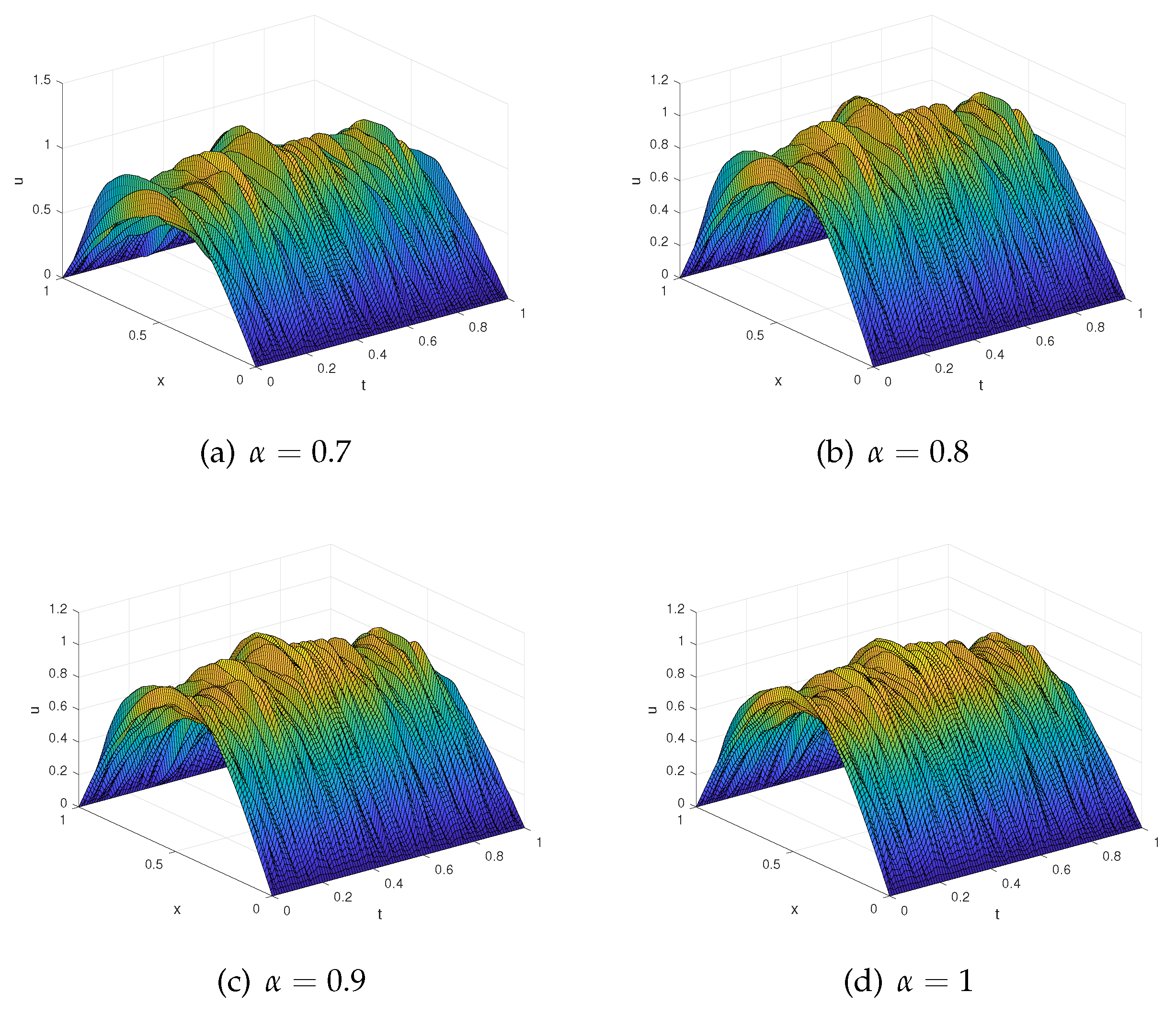
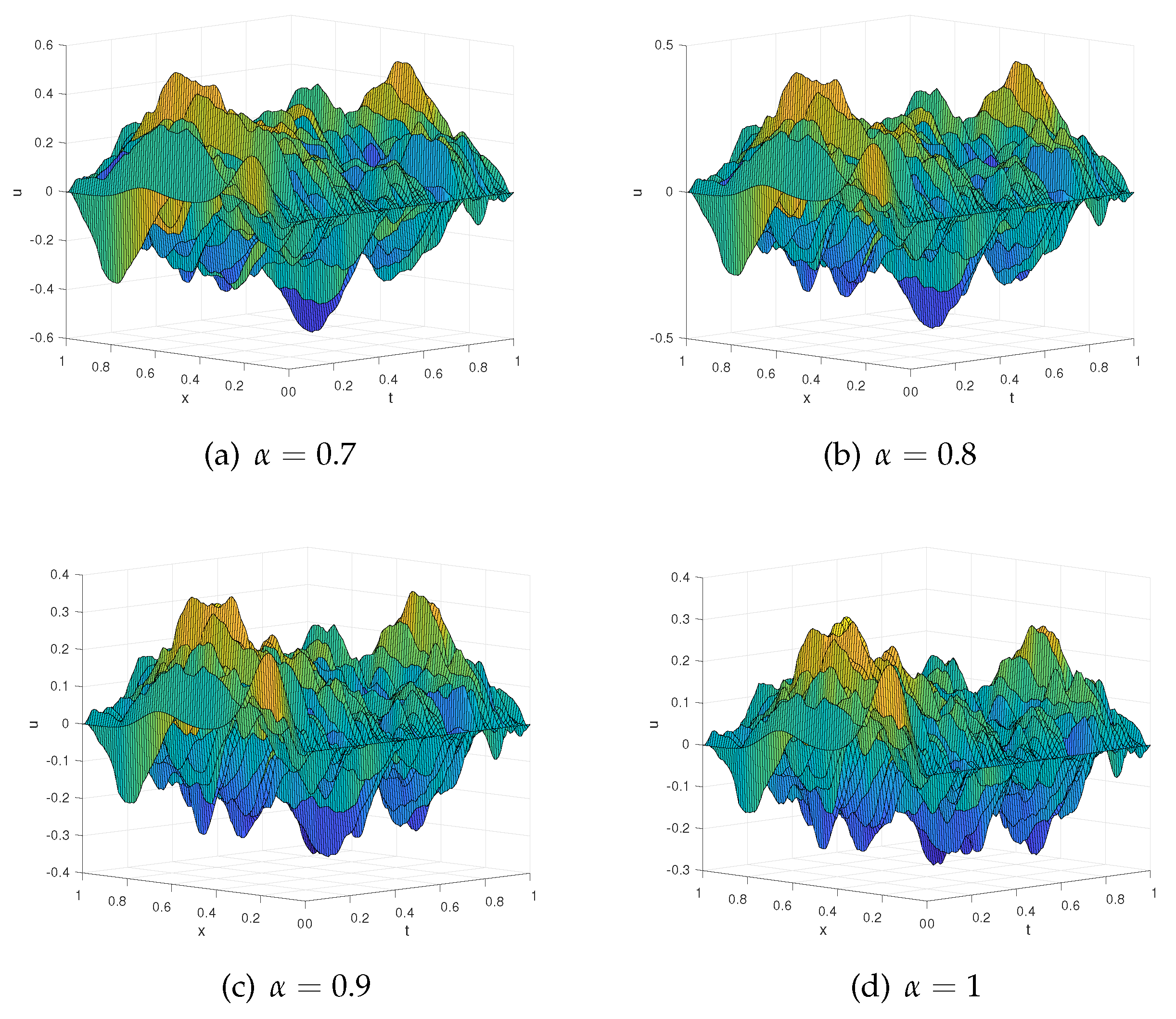
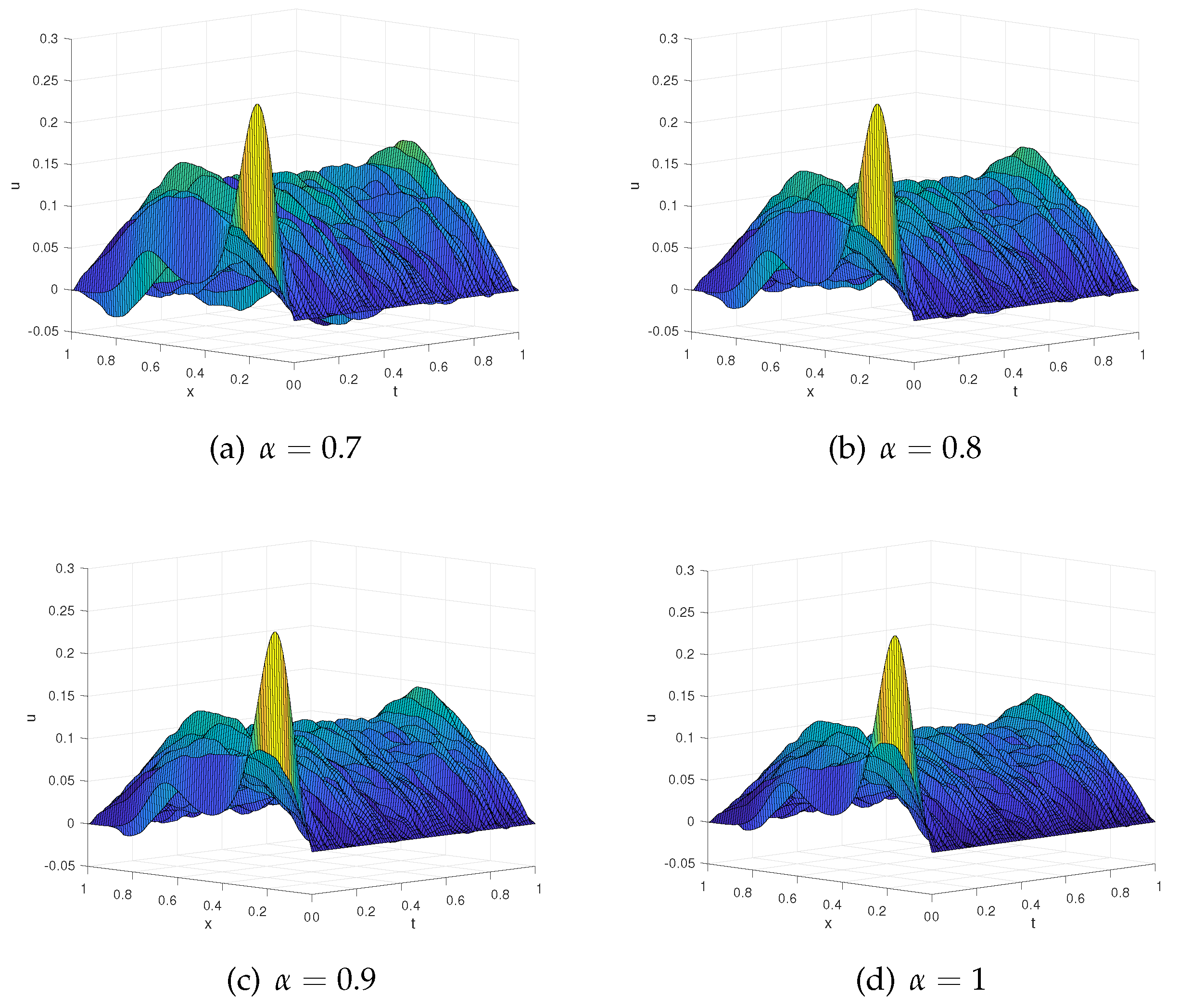
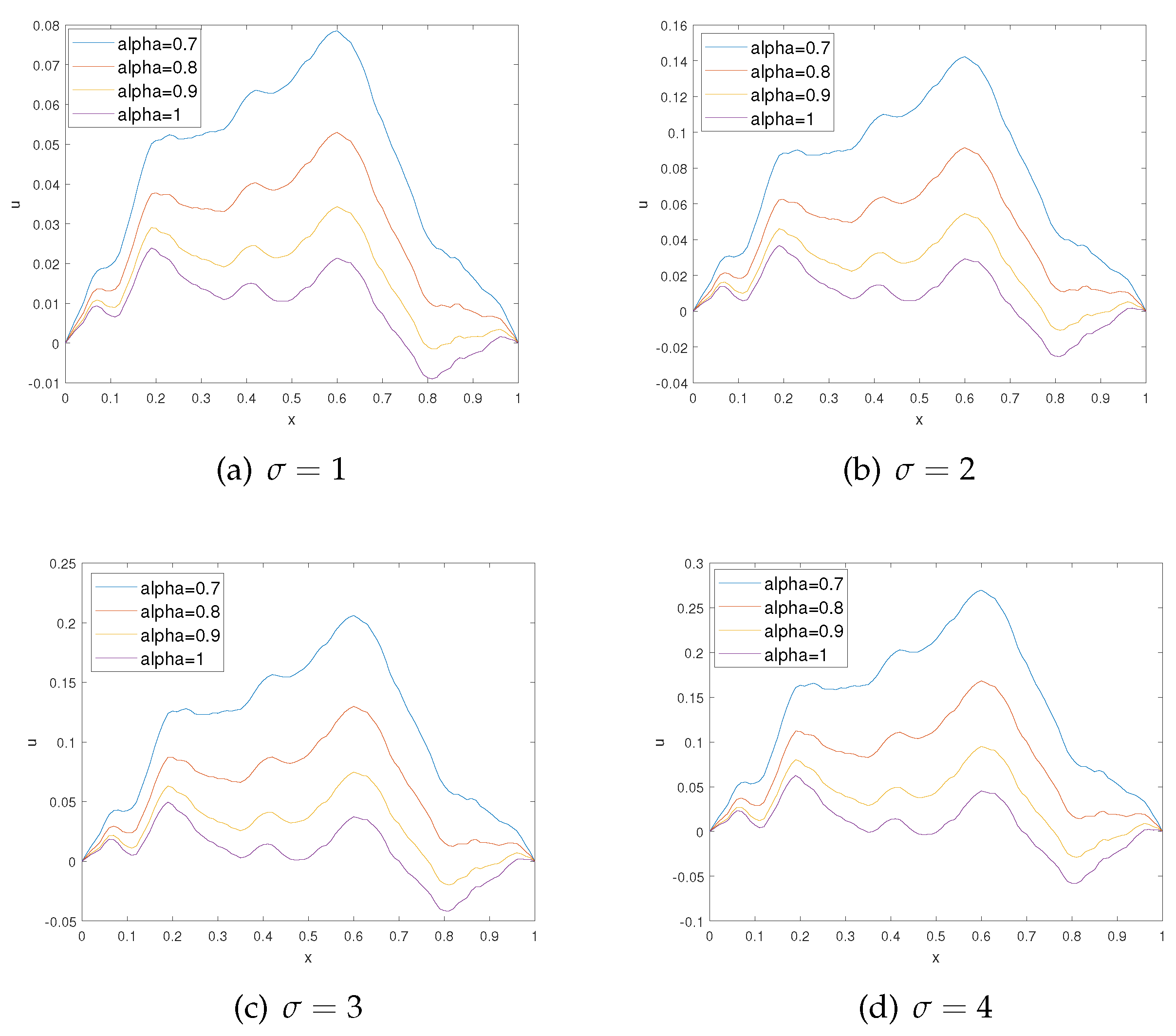
Example 1.

Consider the following SGFDE:

$${\displaystyle \frac{{}^{*}{\partial }^{\alpha }u(x,t)}{{}^{*}\partial t^{\alpha }}}={\displaystyle \frac{{\partial }^{2}u(x,t)}{\partial x^2}}+f(x,t)+\sigma \dot{W}(x,t),0<\alpha <1,0<t<1,0<x<1,$$

(20)

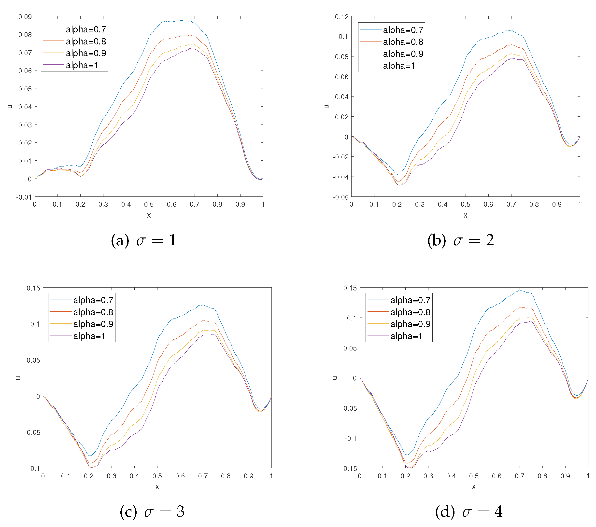
with the initial and boundary conditions: $u(x,0)=sin\left(x\pi \right)$, $u(0,t)=g_1\left(t\right)=0$, and $u(1,t)=g_2\left(t\right)=0$, where $f(x,t)={\displaystyle \frac{2}{\mathsf{\Gamma }(3-\alpha )}}(x^2-x)t^{2-\alpha }+{\pi }^{2}sin\left(x\pi \right)-2t^2$, and ${\displaystyle \frac{{}^{*}{\partial }^{\alpha }u(x,t)}{{}^{*}\partial t^{\alpha }}}$ stand for the GTFD of u(x, t) given by Equation (6). Let $\omega \left(t\right)=1$, $z\left(t\right)=t$, then Equation (20) reduces to a classical FDE.

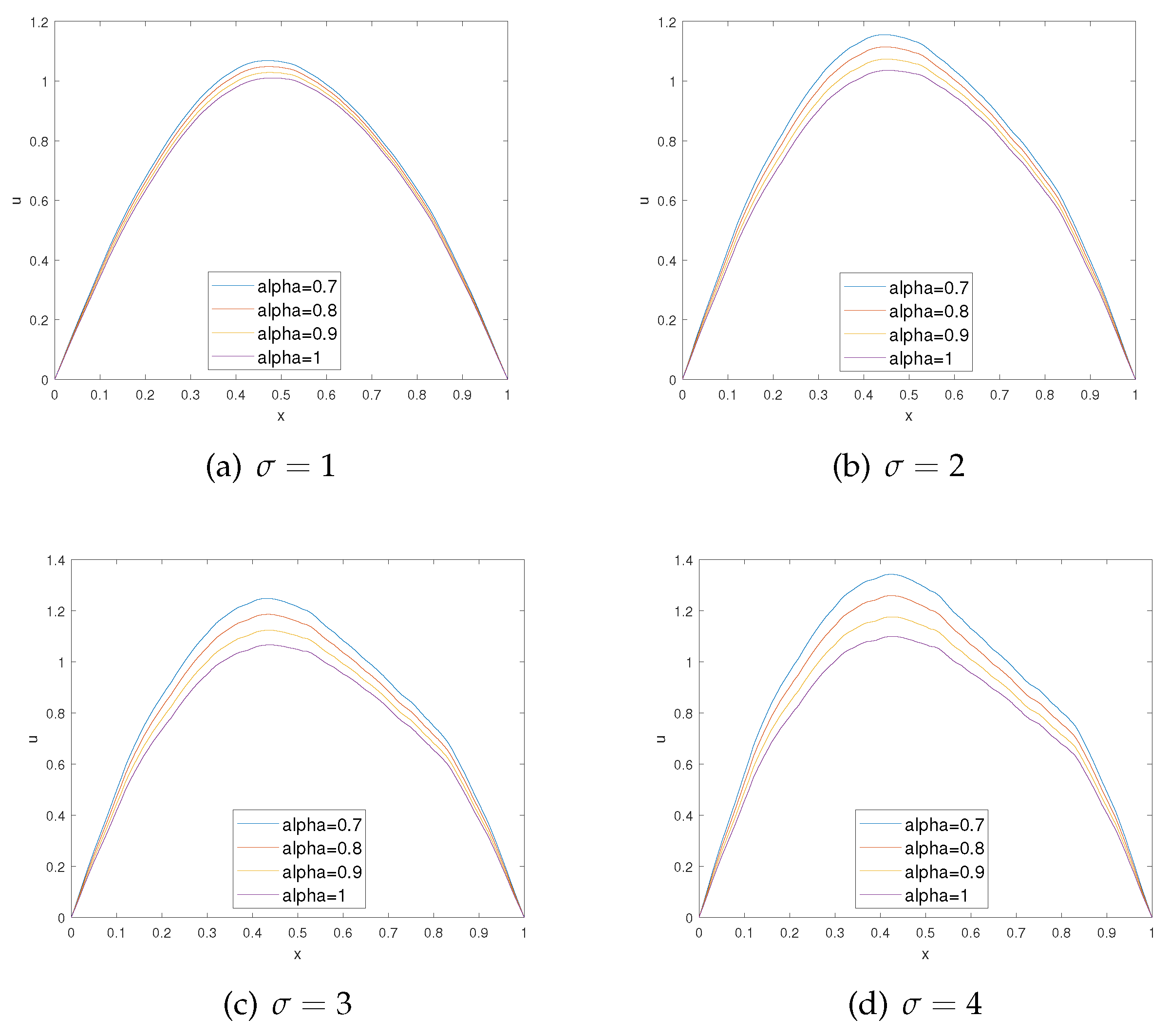
Figure 1 and Figure 2 show the numerical solutions for different values of $\alpha$ and $\sigma$. Figure 3 shows the numerical solutions at $t=0.2$ and different values of $\alpha$ and $\sigma$.

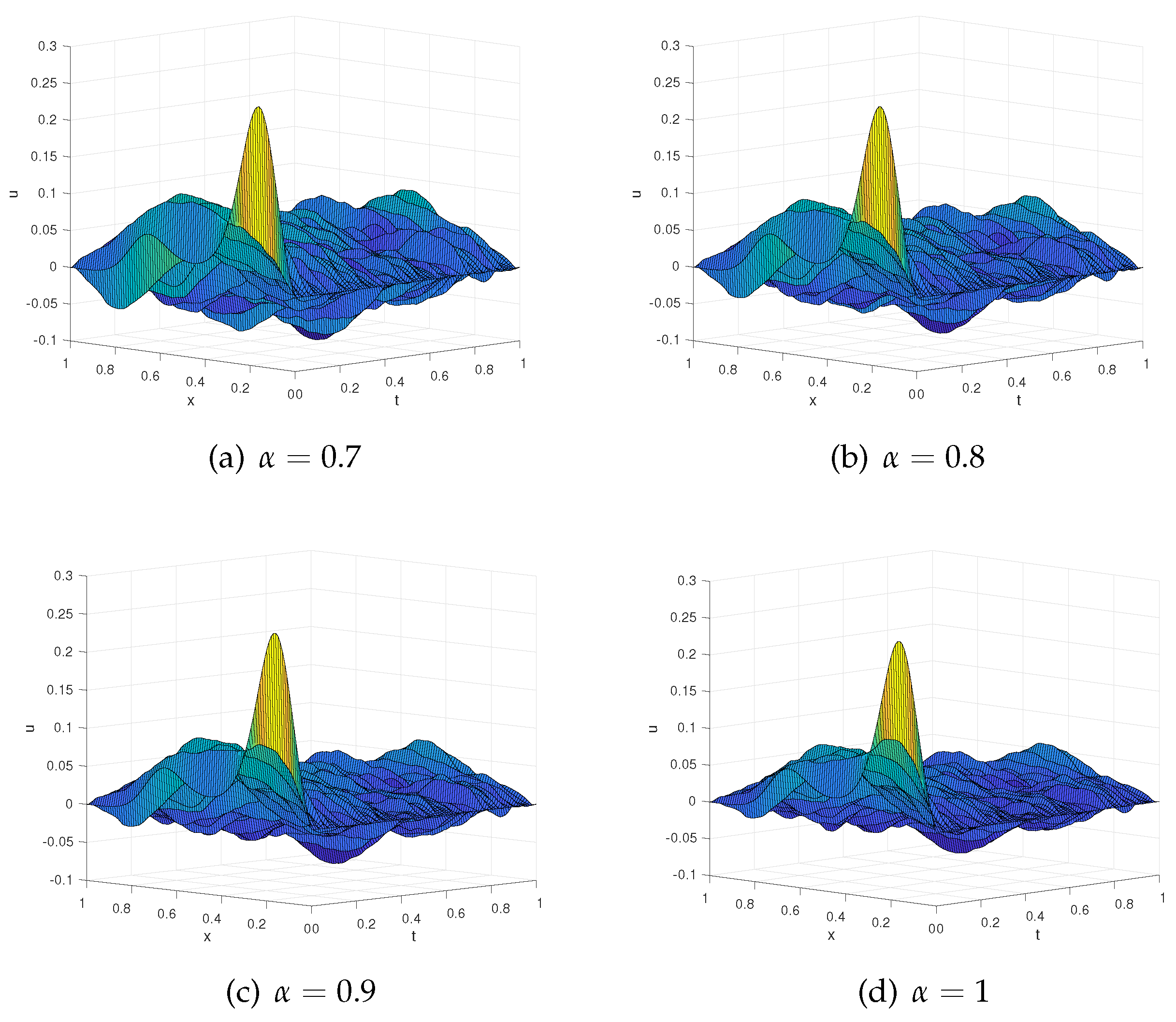
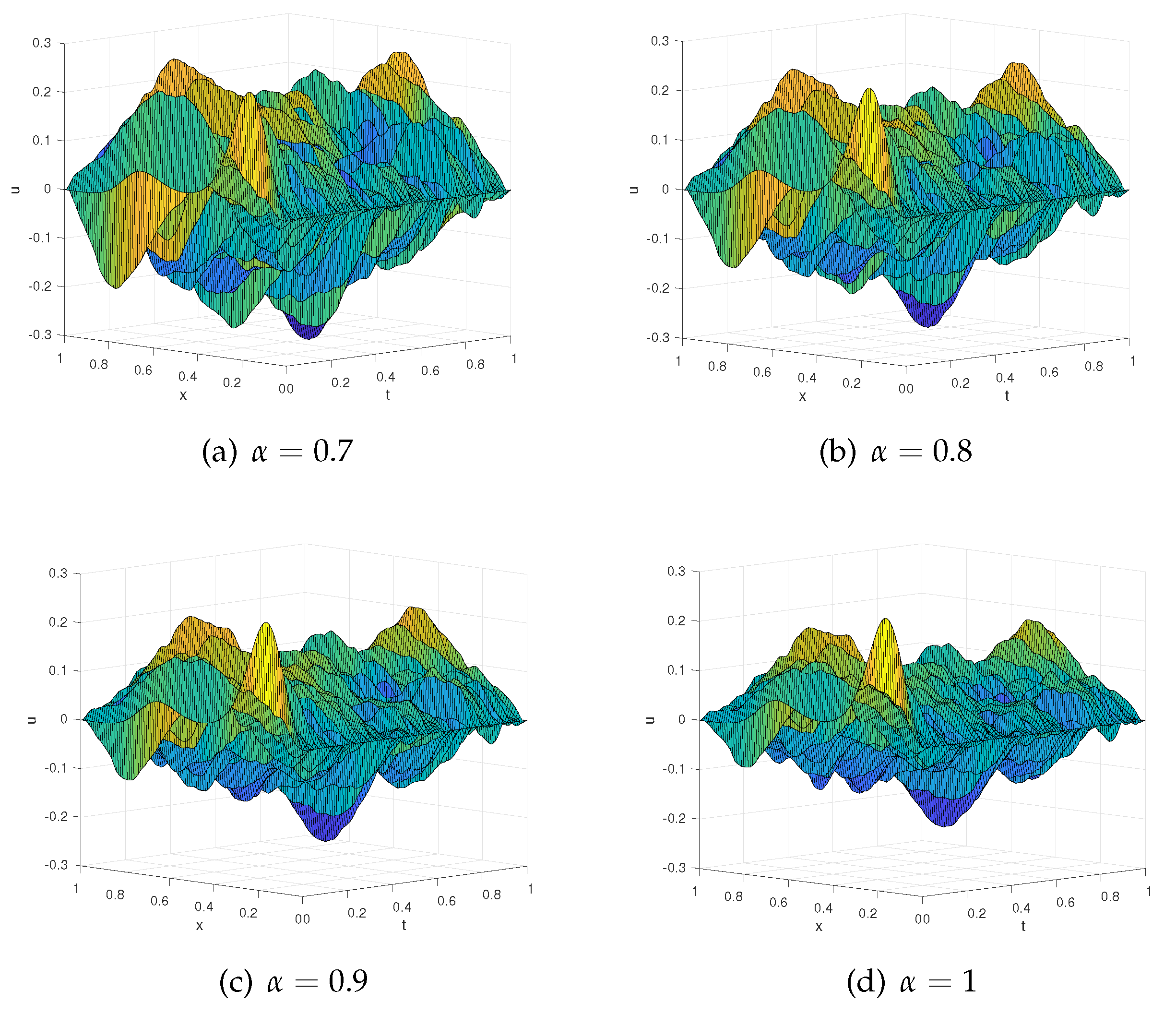
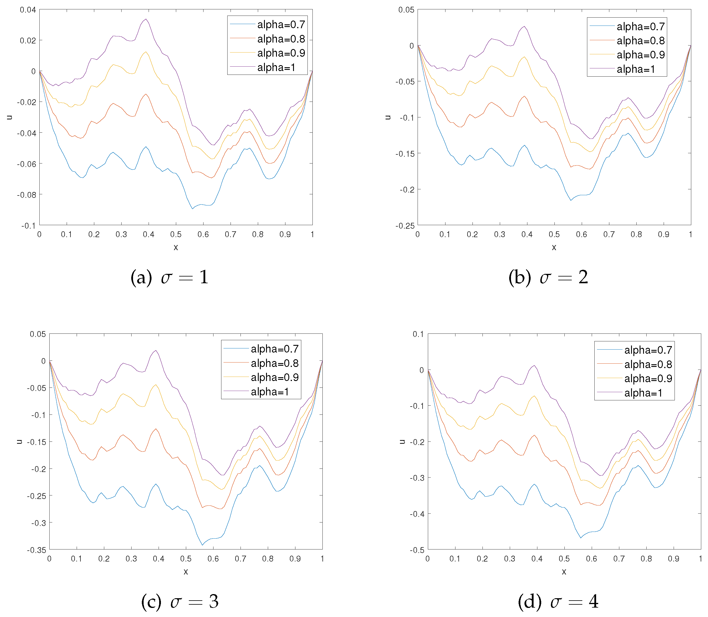
Example 2.

Consider the following SGFDE:

$${\displaystyle \frac{{}^{*}{\partial }^{\alpha }u(x,t)}{\partial t^{\alpha }}}=\nu {\displaystyle \frac{{\partial }^{2}u(x,t)}{\partial x^2}}+f(x,t)+\sigma \dot{W}(x,t),0<t<1,0<x<1,$$

(21)

with $0<\alpha <1$, and $u(0,t)=u(1,t)=0$.

(1) 

$\nu =1.5$, source term $f(x,t)={\displaystyle \frac{(x-1)(t-1)}{2+sin\left(xt\right)}}$, scale function $z\left(t\right)=t$, weight function $\omega \left(t\right)=exp\left(t\right)$, and the initial condition as $u(x,0)=x{(1-x)}^{3}exp(sin\left(3.5\pi x\right))$. We observe that the solutions tend to zero eventually, which is because Equation (7) is a diffusion equation with zero-boundary conditions.

(2) 

$\nu =0.5$, source term $f(x,t)={\displaystyle \frac{(x-1)(t-1)}{2+sin\left(xt\right)}}$, scale function $z\left(t\right)=t$, weight function $\omega \left(t\right)=exp\left(t\right)$, and the initial condition as $u(x,0)=x{(1-x)}^{3}exp(sin\left(3.5\pi x\right))$. Comparison of Figure 4 with Figure 6 shows that when the diffusion coefficient ν reduces, the diffusion becomes slow.

(3) 

$\nu =1.5$, source term $f(x,t)=1$, scale function $z\left(t\right)=t$, weight function $\omega \left(t\right)=exp\left(t\right)$, and the initial condition as $u(x,0)=x{(1-x)}^{3}exp(sin\left(3.5\pi x\right))$. Comparison of Figure 8 with Figure 4 shows that when the source term is a nonzero constant, which means that the energy will be supplied constantly during diffusion, the diffusion will tend to be a nonzero stationary distribution.

Figure 4, Figure 5, Figure 6, Figure 7, Figure 8 and Figure 9 show the numerical solutions for different values of $\alpha$ and $\sigma$ in three cases. Figure 10, Figure 11 and Figure 12 show the numerical solutions at $t=0.2$ and different values of $\alpha$ and $\sigma$ at $t=0.3,0.4$, and $0.45$ in three cases.

6. Conclusions

This article introduces a model to the GFDEs as SGFDEs including a random term. The finite difference method is also used for finding numerical solution of SGFDEs. Numerical examples with plots of the results are depicted to show the efficiency of the proposed method.

References

- Debrabant, K.; Kværnø, A. B-series analysis of stochastic Runge-Kutta methods that use an iterative scheme to compute their internal stage values. SIAM J. Numer. Anal. 2008, 47, 181–203. [Google Scholar] [CrossRef]
- Kloeden, P.; Platen, E. Numerical Solution of Stochastic Differential Equations; Springer: Berlin, Germany, 1999. [Google Scholar]
- Barth, A. A Finite Element Method for Martingale-Stochastic Partial Differential Equations. Commun. Stoch. Anal. 2010, 4, 355–375. [Google Scholar] [CrossRef]
- Mohammed, A.S. Mean Square Convergent Three and Five Points Finite Difference Scheme for Stochastic Parabolic Partial Differential Equations. Electron. J. Math. Anal. Appl. 2014, 2, 164–171. [Google Scholar]
- Soong, T.T. Random Differential Equations in Science and Engineering; Academic Press: New York, NY, USA, 1973. [Google Scholar]
- Alabert, A.; Gyongy, I. On Numerical Approximation of Stochastic Burgers’ Equation. In From Stochastic Calculus to Mathematical Finance; Kabanov, Y., Liptser, R., Stoyanov, J., Eds.; Springer: Berlin, Germany, 2006; pp. 1–15. [Google Scholar]
- Davie, A.M.; Gaines, J.G. Convergence of Numerical Schemes for the Solution of Parabolic Stochastic Partial Differential Equations. Math. Comput. 2011, 70, 121–134. [Google Scholar] [CrossRef]
- Printems, J. On the Discretization in Time of Parabolic Stochastic Partial Differential Equations. ESAIM Math. Model. Numer. Anal. 2001, 35, 1055–1078. [Google Scholar] [CrossRef]
- Diethelm, K. The Analysis of Fractional Differential Equations: An Application-Oriented Exposition Using Differential Operators of Caputo Type; Springer: Berlin, Germany, 2010. [Google Scholar]
- Spanier, J.; Oldham, K.B. The Fractional Calculus; Academic Press: New York, NY, USA, 1974. [Google Scholar]
- Ross, B. The development of fractional calculus 1695-1900. Hist. Math. 1977, 4, 75–89. [Google Scholar] [CrossRef]
- Rossikhin, Y.A. Reflections on two parallel ways in the progress of fractional calculus in mechanics of solids. Appl. Mech. Rev. 2010, 63, 010701. [Google Scholar] [CrossRef]
- Samko, S.G.; Kilbas, A.A.; Marichev, O.I. Fractional Integrals and Derivatives: Theory and Applications; Gordon and Breach: Yverdon, Switzerland, 1993. [Google Scholar]
- Seybold, H.J.; Hilfer, R. Numerical results for the generalized Mittag-Leffler functions. Fract. Calc. Appl. Anal. 2005, 8, 127–139. [Google Scholar]
- Odibat, Z.M. Analytic study on linear systems of fractional differential equations. Comput. Math. Appl. 2010, 59, 1171–1183. [Google Scholar] [CrossRef]
- Odibat, Z.; Momani, S.; Erturk, V.S. Generalized differential transform method: Application to differential equations of fractional order. Appl. Math. Comput. 2008, 197, 467–477. [Google Scholar] [CrossRef]
- Xu, Y.; He, Z.; Agrawal, O. Numerical and analytical solutions of new generalized fractional diffusion equation. Comput. Math. Appl. 2013, 66, 2019–2029. [Google Scholar] [CrossRef]
- Agrawal, O. Some generalized fractional calculus operators and their applications in integral equations. Fract. Calc. Anal. Appl. 2012, 15, 700–711. [Google Scholar] [CrossRef] [Green Version]
- Kilbas, A.; Srivastava, H.; Trujillo, J. Theory and Applications of Fractional Differential Equations; Elsevier: Amsterdam, The Netherlands, 2006. [Google Scholar]
- El-Tawil, M.A.; Sohaly, M.A. Mean square convergent three points finite difference scheme for random partial differential equations. J. Egypt. Math. Soc. 2012, 20, 188–204. [Google Scholar] [CrossRef]
- Ekström, S.-E.; Furci, I.; Garoni, C.; Manni, C.; Serra-Capizzano, S.; Speleers, H. Are the eigenvalues of the B-spline IgA approximation of −Δu = λu known in almost closed form? Numer. Linear Algebra Appl. 2018. [Google Scholar] [CrossRef]
- Serra-Capizzano, S. On the extreme spectral properties of symmetric Toeplitz matrices generated by L1 functions with several global minima/maxima. BIT 1996, 36, 135–142. [Google Scholar] [CrossRef]
- Smith, G.D. Numerical Solution of Partial Differential Equations: Finite Difference Methods; Oxford University Press: Oxford, UK, 1985. [Google Scholar]
Figure 1.
The approximation solutions of Example 1 with .
Figure 2.
Figure 3.
Figure 4.
The approximation solutions of Example 2 (case (1)) with .
Figure 5.
Figure 6.
The approximation solutions of Example 2 (case (2)) with .
Figure 7.
Figure 8.
The approximation solutions of Example 2 (case (3)) with .
Figure 9.
Figure 10.
Figure 11.
Figure 12.
© 2018 by the authors. Licensee MDPI, Basel, Switzerland. This article is an open access article distributed under the terms and conditions of the Creative Commons Attribution (CC BY) license (http://creativecommons.org/licenses/by/4.0/).
Share and Cite
MDPI and ACS Style
Sepahvandzadeh, A.; Ghazanfari, B.; Asadian, N. Numerical Solution of Stochastic Generalized Fractional Diffusion Equation by Finite Difference Method. Math. Comput. Appl. 2018, 23, 53. https://doi.org/10.3390/mca23040053
AMA Style
Sepahvandzadeh A, Ghazanfari B, Asadian N. Numerical Solution of Stochastic Generalized Fractional Diffusion Equation by Finite Difference Method. Mathematical and Computational Applications. 2018; 23(4):53. https://doi.org/10.3390/mca23040053
Chicago/Turabian StyleSepahvandzadeh, Amaneh, Bahman Ghazanfari, and Nader Asadian. 2018. "Numerical Solution of Stochastic Generalized Fractional Diffusion Equation by Finite Difference Method" Mathematical and Computational Applications 23, no. 4: 53. https://doi.org/10.3390/mca23040053