Rapid Solution of Optimal Control Problems by a Functional Spreadsheet Paradigm: A Practical Method for the Non-Programmer


ExcelWorks LLC, Sharon, MA 02067, USA
Math. Comput. Appl. 2018, 23(4), 54; https://doi.org/10.3390/mca23040054
Submission received: 29 August 2018
/
Revised: 24 September 2018
/
Accepted: 26 September 2018
/
Published: 28 September 2018
(This article belongs to the Special Issue Optimization in Control Applications)
Abstract
:We devise a practical and systematic spreadsheet solution paradigm for general optimal control problems. The paradigm is based on an adaptation of a partial-parametrization direct solution method which preserves the original mathematical optimization statement, but transforms it into a simplified nonlinear programming problem (NLP) suitable for Excel NLP solver. A rapid solution strategy is implemented by a tiered arrangement of pure elementary calculus functions in conjunction with Excel NLP solver. With the aid of the calculus functions, a cost index and constraints are represented by equivalent formulas that fully encapsulate an underlining parametrized dynamical system. Excel NLP solver is then employed to minimize (or maximize) the cost index formula, by varying decision parameters, subject to the constraints formulas. The paradigm is demonstrated for several fixed and free-time nonlinear optimal control problems involving integral and implicit dynamic constraints with direct comparison to published results obtained by fundamentally different methods. Practically, applying the paradigm involves no more than defining a few formulas using basic Excel spreadsheet skills.
1. Introduction
Many researchers and academics often need to solve optimal control problems that are frequently postulated in various engineering, social, and life sciences [1,2,3]. An optimal control problem is concerned with finding control functions, (or policies), that achieve optimal trajectories for a set of controlled differential state variables. The optimal trajectories are determined by solving a constrained dynamical optimization problem, such that a cost index is minimized (or maximized), subject to constraints on state variables and control functions. Mathematically, an optimal control problem may be stated generally as follows (bold symbols indicate vector-valued functions):
Find control functions and corresponding state variables which minimize (or maximize) the cost index
subject to
with initial conditions
and end conditions and bounds
In the formulation (1)–(5), the generally nonlinear H, and G are scalar functions, whereas F, Q and S are vector valued functions. Typically, either H or Q are specified but not both in the same problem. Common forms of Q and S are end conditions on the state variables, , and bound constraints on the controls, respectively. More general forms of S considered in this paper include algebraic and integral constraints involving derivatives. The matrix M in (2) offers an optional coupling of states’ temporal derivatives by a mass matrix which may be singular. If M is singular, the equation system (2) is differential algebraic, or DAE. For uncoupled derivatives, M is the identity matrix which can be omitted. Furthermore, , which denotes the final time, may be fixed or free.
Numerical solution strategies for (1)–(5) can be classified into two approaches: indirect and direct methods. Indirect methods employ Pontryagin’s minimum principle to transform the problem into an augmented Hamiltonian system requiring the solution of a boundary value problem which may be hard to solve [4,5]. On the other hand, direct method approaches transform the original optimal control problem into a nonlinear programming problem which can be solved by various established NLP packages. The transformation is carried out via a discretization of the control and the state functions on a time grid using some form of a collocation method [4,6,7]. Complete discretization of the state and control functions eliminate the need to iteratively solve the inner initial value problem (IVP) (2) but at the expense of a large numbers of decision variables for the NLP solver. Other direct approaches rely only on a partial parametrization for the control functions using piecewise constant or higher order polynomial approximations [8]. In this approach, the inner IVP must be solved repeatedly by the outer NLP algorithm while searching for the optimal parameter vector. Except for the most trivial cases, optimal control problems are inherently nontrivial to solve. They typically require a level of programming fluency, in addition to a good understanding of the general structure of the solution strategy, and the various solvers required to implement it [9].
In [10], the author introduced a practical spreadsheet method for solving a class of optimal control problems using basic spreadsheet skills. The method utilized two elementary calculus functions: an initial value problem solver and a discrete data integrator from an available Excel calculus Add-in [11] in conjunction with Excel intrinsic NLP solver to formulate a partial-parametrization direct solution strategy. With the aid of the calculus functions, a cost index was represented by an equivalent formula that fully encapsulated a control-parametrized inner IVP (2)–(3). Excel NLP solver was employed next for minimizing (or maximizing) the cost index formula, by varying a decision parameter vector, subject to bounds constraints on state and control variables. The method proved effective at solving several nonlinear optimal control problems reproduced from Elnagar and Kazemi [6] who employed a full-parametrization direct method using pseudo-spectral approximation and NLPQL optimization software.
This research paper aims at generalizing the method introduced in [10] for more general formulations of optimal control than previously considered. More specifically, this paper demonstrates a systematic solution strategy formulated by the aid of various elementary calculus functions, for optimal control problems involving one or more of the following conditions: dependence on higher order derivatives of state or control variables in the cost index and constraints; integral and algebraic dynamic constraints; as well as implicit inner IVP. In addition, this paper investigates convergence and error control of the method, and provides direct comparison of optimal trajectories with published solutions obtained by fundamentally different methods.
It should be noted that the solution strategy formulation pursued in this research, although founded on a common approach, follows closely the original mathematical problem statement, and thus implementation of the strategy varies according to the given problem. Therefore, the paper gives considerable emphasis on the application of the method using four representative problems selected from various applications. Results presented in Section 3 are remarkable, in terms of convergence, agreement with published solutions, and notably, the minimal effort required to obtain them with basic spreadsheet formulas.
In view of traditional spreadsheet applications, the devised solution strategy represents a leap in the utilization of the spreadsheet for solving general optimal control problems. The strategy departs markedly from prior spreadsheet approaches [12,13] by shifting the effort from a low-level detailed algorithmic implementation to a high-level problem modeling. Prior approaches utilized the spreadsheet explicitly as the computational grid for the discretization and solution of the inner IVP. This effectively constrained the scope to rather simple problems that can be easily discretized with an explicit differencing scheme suitable for the spreadsheet. In contrast, we employ a set of pure calculus functions for computing integrals, derivatives and solving differential equations as the building blocks for a direct solution method. The calculus functions, described in Appendix A, utilize adaptive algorithms which are independent of the spreadsheet grid and thus suitable for a general class for nonlinear stiff problems. The calculus functions are utilized in formulas just like intrinsic math functions based on a simple input/output model. In essence, the calculus functions represent a natural extension of the built-in spreadsheet math functions with the allowance that some of their input arguments are functions themselves and not just static values.
The reminder of this paper is organized as follows: In the next section, we present an outline of the general steps required to implement the direct spreadsheet solution strategy, and discuss sources of errors that impact convergence and accuracy of the solution as well as possible remedies. In Section 3, we apply the method for solving four different optimal control problems selected to demonstrate the various conditions outlined earlier. Direct comparisons of optimal trajectories obtained by the method versus published solutions obtained by fundamentally different approaches are also provided. In addition, effects of parametrization order and error control are investigated in some problems. Section 4 presents concluding remarks as well as directions for future research. Detailed descriptions of the various calculus functions utilized in this work are included in Appendix A.
2. Mechanics of Spreadsheet Direct Method
The solution strategy is based on an adaptation of the control-parametrization direct approach [4,8] by an analogous spreadsheet functional formulation. The building blocks of the functional formulation are a set of calculus spreadsheet functions [11,14] which integrate with the spreadsheet, like intrinsic pure math functions, but also accept formulas as a new type of argument for solving problems in integral, algebraic, and differential calculus. For example, an integration function accepts a formula and limits as inputs, and it outputs an accurate integral value much like an intrinsic math function accepts a number and computes its square root. Specifically, we make use of the following functions from a calculus Add-in [11]:
- Initial value problem solver, IVSOLVE, using RADAU5 an implicit 5th-order Runge-Kutta algorithm with adaptive time step [15].
- Discrete data Integrator, QUADXY, using cubic splines [16].
- Discrete data differentiator, DERIVXY, using cubic splines [16].
- Formula integrator, QUADF, using Gauss quadrature with adaptive error control [17].
The functions are utilized in combination with Excel NLP solver, which is based on the Generalized Reduced Gradient algorithm based on Lasdon and Waren [18]. A detailed description of the calculus functions usage, and respective algorithms are given in Appendix A. The critical characteristic of the calculus functions which permits their seamless utilization with the NLP solver in a functional paradigm, is the mathematical purity property. The calculus functions do not modify their inputs, and produce no side effects in the spreadsheet. They only compute and display a solution result in their allocated spreadsheet memory cells. The authority to modify the inputs to the calculus functions, via changes to the decision parameter vector, is confined to the outer NLP solver command.
Below, we describe the main elements of the solution strategy introduced originally in [10] but generalized in this work for solving general optimal control problem (1)–(5) with the aim of supporting the various conditions outlined earlier.
2.1. Solution Strategy
The strategy comprises three ordered steps which are implemented by the aid of calculus functions:
In the first step, we obtain an initial solution to the inner IVP (2)–(3), based on suitable parametrization for the control functions with initial guesses for the unknown parameters and a final time for free-time problems. The unknown parameters and the final time constitute the decision variables for the final optimization step by the outer NLP solver. Any prior information about the controls should be incorporated in the specified parametrization. Absent any information, a low-order polynomial is often an adequate choice. The initial IVP solution is obtained by the calculus function IVSOLVE which displays the state variables, , in an allocated array of the spreadsheet at uniform output time points. It should be noted that output time grid is determined by the number of rows in the allocated output array but is, otherwise, unrelated to the accuracy of the computed solution. To display a finer output time grid, a larger output array should be allocated. However, the resolution of the output time grid affects the accuracy of the computed integrals for the cost index and any integral constraints which is discussed in Section 2.2. Optional parameters to IVSOLVE could also be used to control or specify the output time points.
In the second step, we construct an analogous formula for the cost index (1) dependent on the initial solution outputted by IVSOLVE. The cost index may depend on , the control values, , as well as first and higher order derivatives of the state variables and controls. Values for , and higher derivatives are readily generated using the specified parametrized formula for a control . The spreadsheet is particularly suited for such computations using its AutoFill feature. On the other hand, values for the state variables derivatives and are not readily available and must be approximated by differentiating values obtained by IVSOLVE. We accomplish this task by the aid of a discrete data differentiator calculus function DERIVXY which computes derivatives using cubic splines to model the best function described by . With all the necessary values obtained, we proceed to defining an analogous formula for the cost index, which is typically defined as a continuous time integral of an algebraic integrand. The devised method is to sample the integrand expression using the obtained values for the states, controls and their derivatives, followed by employing a discrete data integrator calculus function QUADXY to integrate a cubic-spline fit function through the sampled integrand. Depending on a particular problem formulation, it may be necessary to define additional formulas to represent constraints equations (5) that may be present. Such formulas can often be constructed in a similar way to the cost index formula using appropriate calculus functions. In particular, we shall demonstrate in Section 3 using an additional formula integrator function QUADF to define an integral constraint formula.
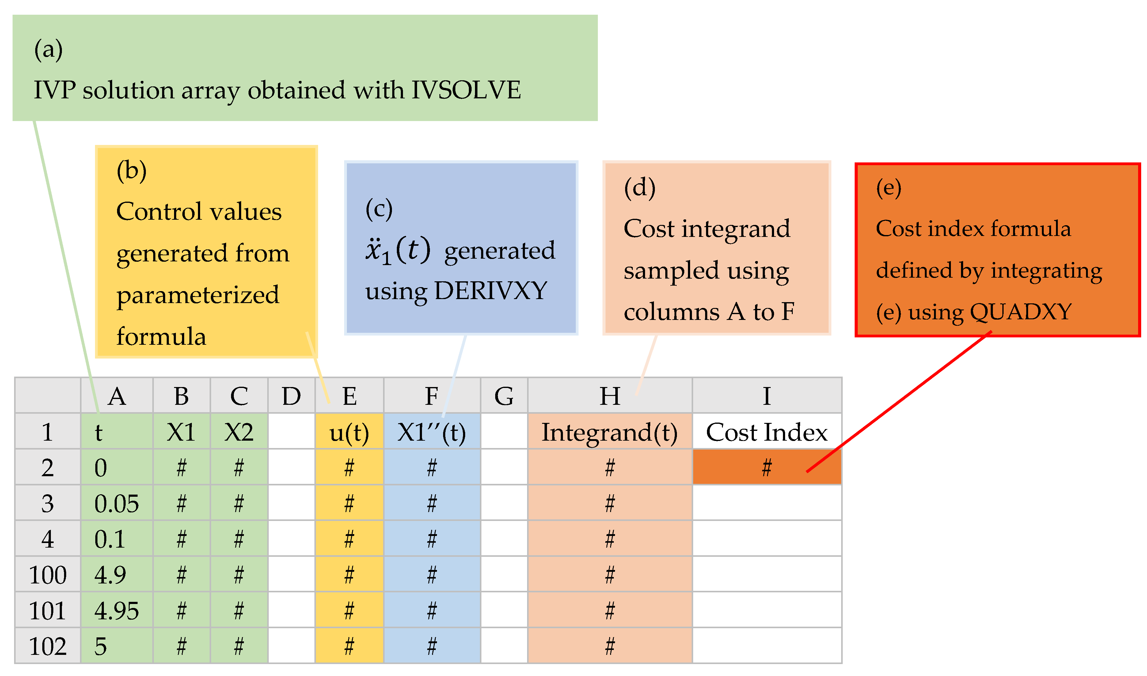
Figure 1 illustrates the aforementioned steps applied to an optimal control problem with one control and two state variables. An initial IVP solution, which is dependent on a decision parameters vector, is obtained with IVSOLVE in an array (Figure 1a). Values for the control, , and any needed state derivatives such as , are generated in additional columns (Figure 1b,c) at the time values of the IVP solution. Next, the cost index integrand expression is sampled at the IVP solution times (Figure 1d), and the sample is then integrated to define the cost index formula (Figure 1e). The generated values interdependence hierarchy ensures that any change to the decision parameters vector, such as by an outer NLP solver, will trigger reevaluation of the cost index formula in the proper order shown in the figure. The cost index formula thus fully encapsulates the inner IVP problem.
In the last step, we configure Excel NLP solver to minimize (or maximize) the cost index formula by varying the decision parameters vector subject to bounds, end conditions and other present constraints. Bound constraints on , as well as end point constraints on , are imposed directly on the corresponding values in the IVP solution array. More general constraints are imposed on additional formulas constructed in step 2 as needed. The three steps are demonstrated on several examples in the next section.
2.2. Convergence and Error Control
Two sources of errors are introduced by the spreadsheet method with respect to the original problem. The first error is introduced by restricting the space of admissible control functions to a finite-dimensional space, for example, variable-order polynomials up to a fixed degree. For some problems, it may not be possible to find a solution if the optimal control, in fact, lies outside the admissible space. The second source of error is introduced by the calculus numerical algorithms. This error can be further split into two sources. The error associated with solution of the inner IVP, and the error associated with integration (or differentiation) of discrete data sets generated from the IVP solution. The first error is bounded by the tolerances specified for IVSOLVE algorithm. The second error impacts the accuracy of the computed integral for the cost index. Under the assumption that the discrete data describe a smooth curve, the computed integral by QUADXY using cubic splines is generally quite accurate. However, it may be further improved by any of the following acts.
- Increasing the size of the data set by increasing the number of rows of the allocated IVP solution array to output a finer time grid.
- Supplying optional slopes at the end points of the curve to the calculus function when available. The slopes may be derived analytically from the integrand expression and can improve the accuracy of the spline fit near the curve edges.
- Using nonuniform output time points clustered near rapidly-varying regions of the state trajectories. This can be controlled via optional arguments to IVSOLVE including supplying exact values for the output time points.
In practice, we have found that the parametrization order and the starting guess for unknown parameters to be the most important factors influencing convergence. We have generally used polynomials up to 5th order which have performed reasonably well. On the other hand, increasing the output array for IVP solution beyond a reasonable size, on the order of 100 uniform subdivisions for the time interval, has not generally resulted in a consistent or significant improvement of the result. In the examples in the next section, we shall demonstrate the effects of both increasing the parametrization order and reducing the output time interval.
3. Illustrative Optimal Control Problems
In the following subsections we apply the method to four different optimal control problems representing various engineering applications and compare the optimal trajectories with published solutions. The computations were carried out on a standard laptop computer with an Intel i7 four-core processor at 2.70 GHz running Microsoft Windows 10 and Excel 2016 with ExceLab calculus add-in [11], which enables the calculus function in Excel. A supplementary Excel workbook containing the solved examples is available for downloading from the publisher.
3.1. Minimum Energy Shape: Hanging Chain
The first example is concerned with finding the shape of a chain of length L suspended between two points, such that its total energy is minimized. We state the problem as described in [19] with L = 4, below:
Find u(t) which minimizes the total energy cost index
subject to the chain length constraint
and the end conditions
Note that in this problem formulation, the inner IVP is implicitly defined by the integral constraint (7). Dolan et al. [19] reformulated the problem, via variable substitution, as a standard optimal control problem subject to a system of explicit differential equations and solved it by a direct approach. Discretization was done using a uniform time step and the trapezoidal rule for the integration. Results for the AMPL implementation were reported using several solvers including KNITRO and LOQO. The best cost index was found at 5.06852 starting from a quadratic approximation and using a grid of 800 nodes. Our spreadsheet solution below is formulated based on the original problem statement (6)–(9).
3.1.1. Solution by Direct Spreadsheet Method
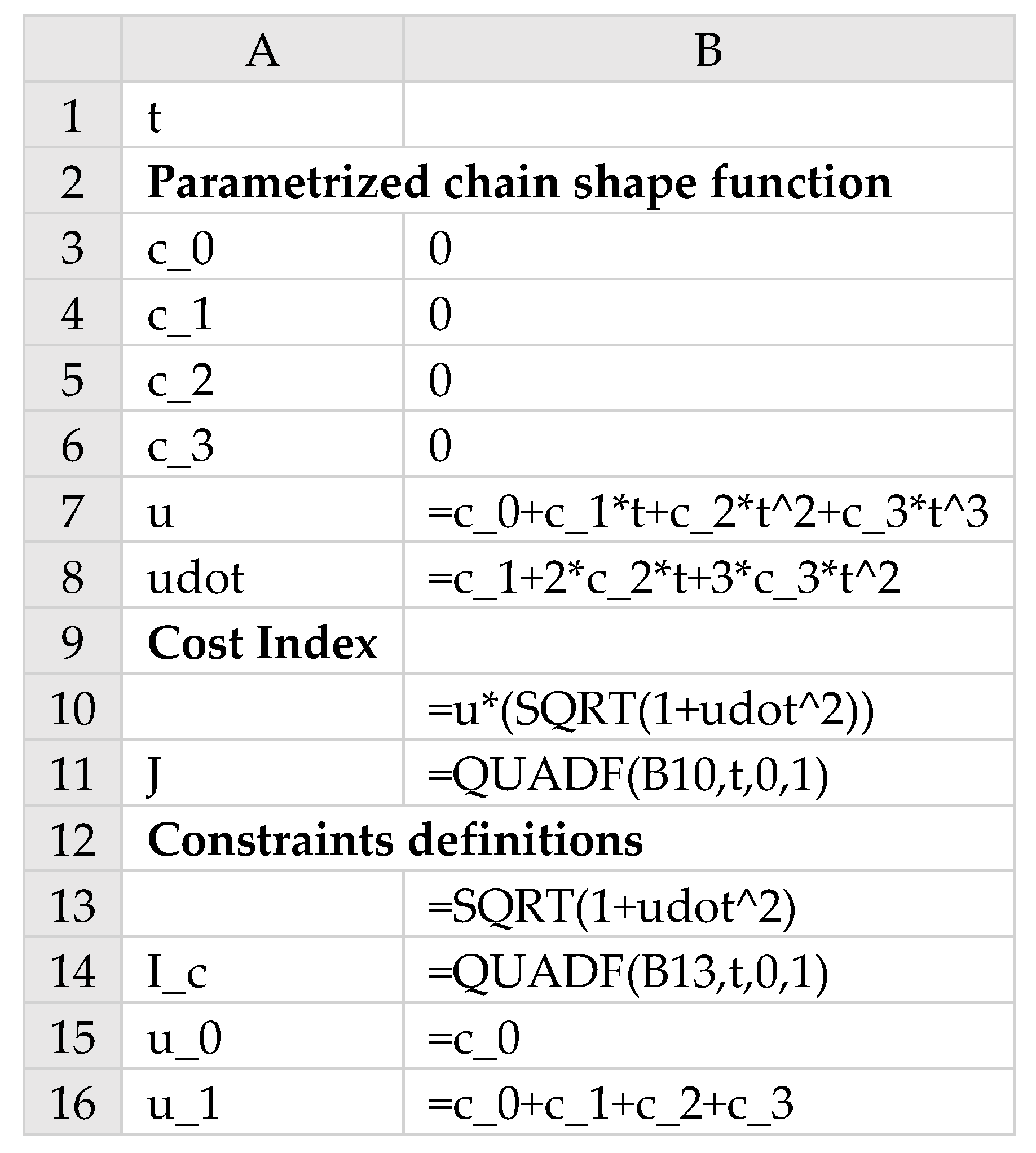
Referring to Figure 2, we setup problem (6)–(9) in Excel using named variables with labels listed in column A. The shape function u(t) was parametrized using a 3rd order polynomial with unknown coefficients c_0, c_1, c_2 and c_3 as shown by formula B7. In B15 and B16, formulas for the initial and final values, u(0) and u(1) were defined by evaluating B7 at time equal zero and one (these formulas are used later to impose the constraints (8)–(9)). An additional formula was defined in B8, (named udot), for the shape function derivative, by differentiating B7 with respect to time. Next, we defined the cost index integral (6), by using the integration calculus function QUADF as shown in B11. The first parameter to QUADF is the integrand which is defined by the equivalent formula in B10. The 2nd parameter is the variable of integration t, and the 3rd and 4th parameters are the integration limits. Likewise, with the aid of QUADF, we defined the constraint integral (7) as shown in B14 (named I_c). This completed the model needed to run Excel NLP solver.
3.1.2. Results and Analysis
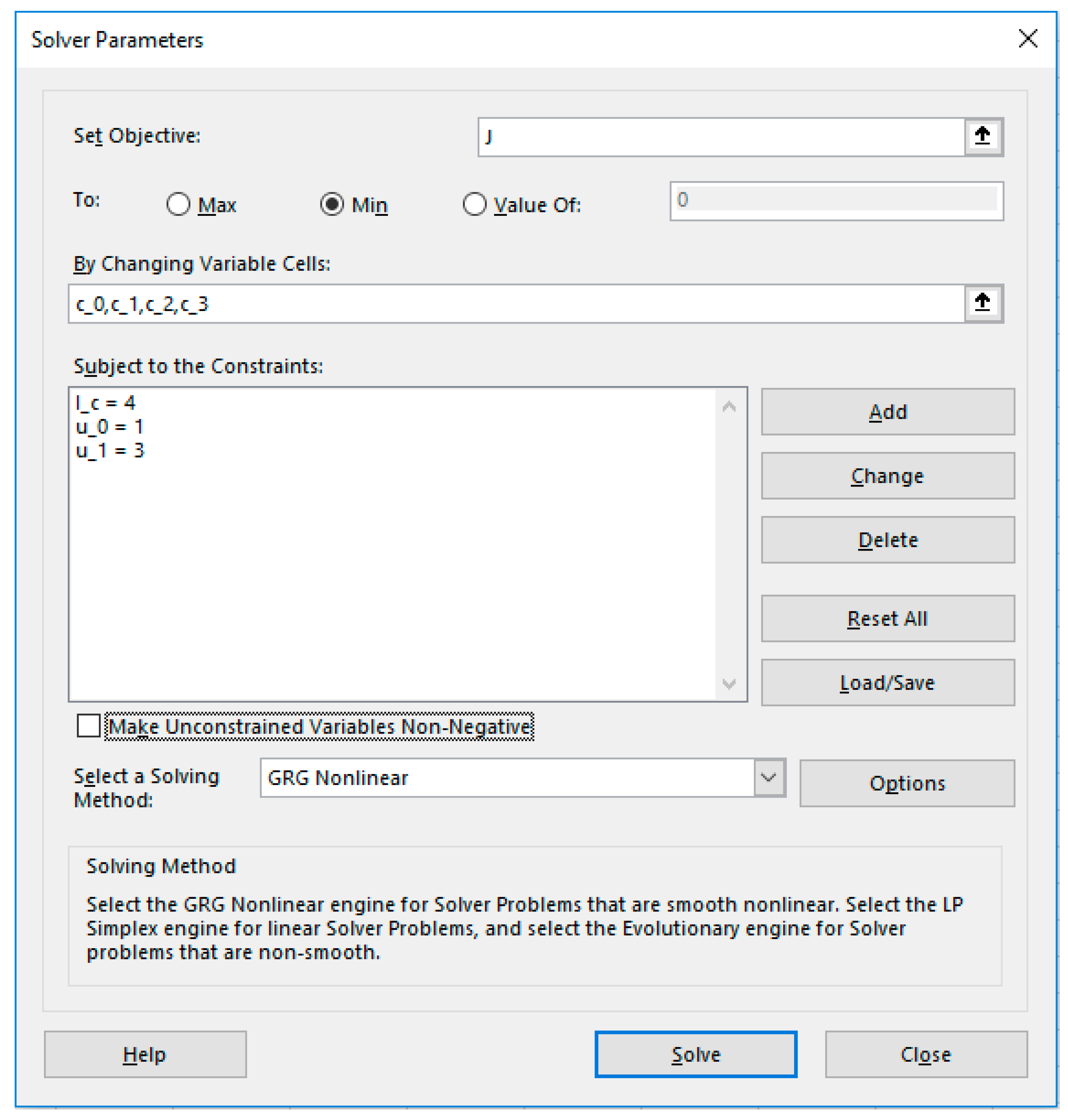
Excel NLP solver is invoked from the Data tab on Excel Ribbon and displays a dialog to enter the problem objective, variables and constraints. Figure 3 shows the inputs for problem 3.1 in which the objective J (B11), was selected to be minimized, by varying the parameters c_0, c_1, c_2 and c_3, subject to the three constraints: I_c = 4, corresponding to (7); u_0 = 1, corresponding to (8); and u_1 = 3, corresponding to (9).
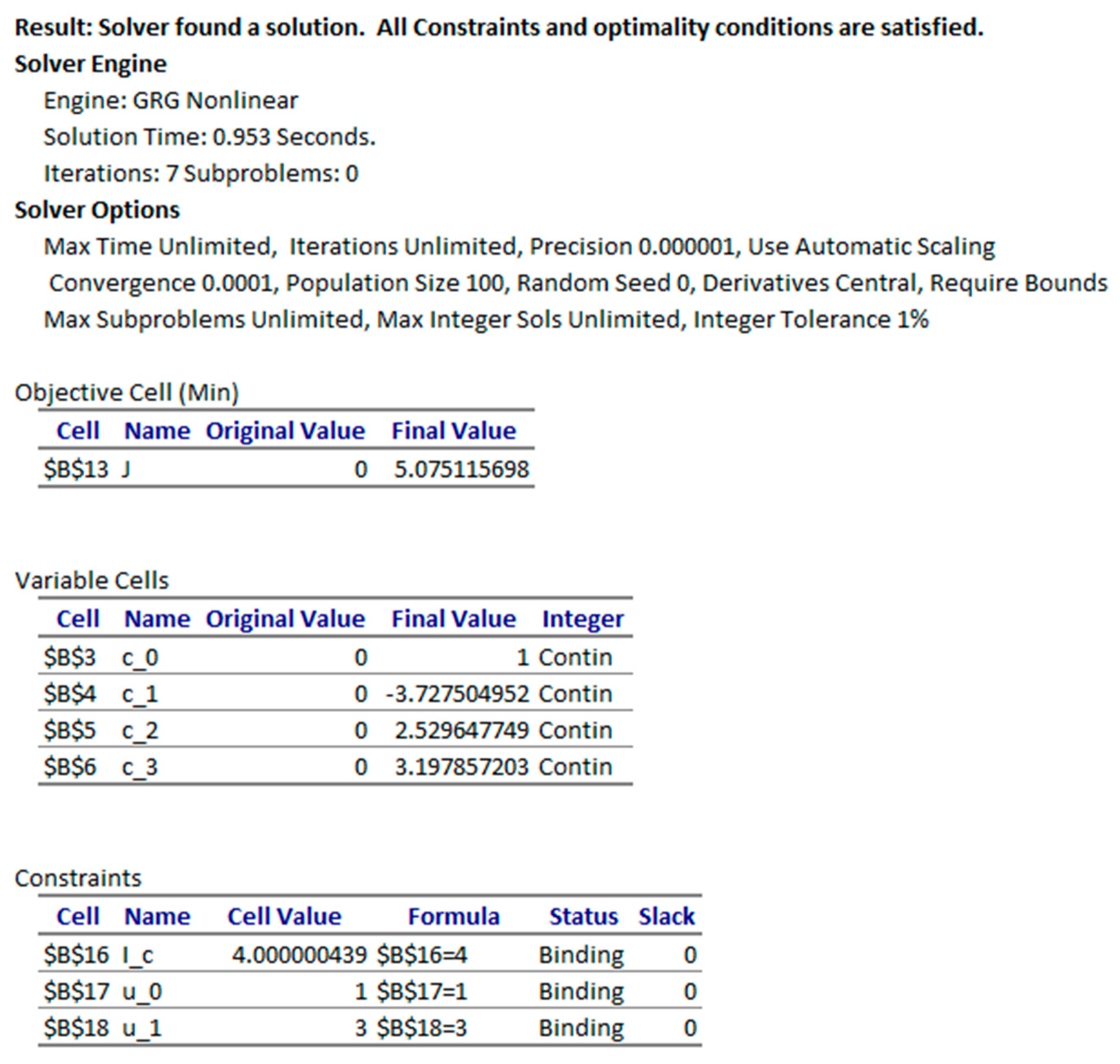
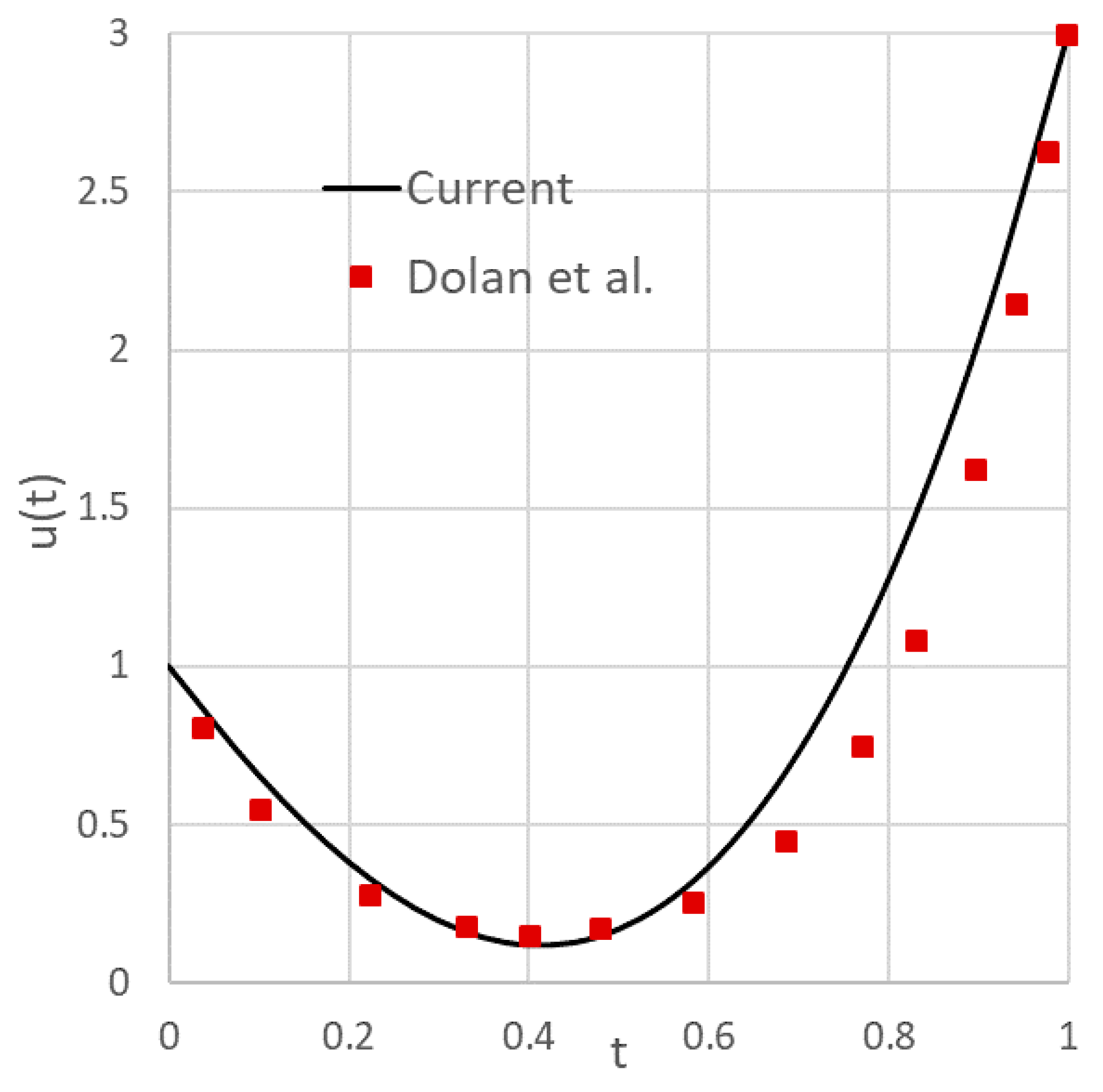
The solver converged, starting from a zero guess for the parameters in less than a second to the result shown in Figure 4 with a final cost index of 5.0751. The optimal shape function u(t) is plotted in Figure 5 together with digitally-read values from the plot published in [19].
The difference between the value reported by Dolan et al. [19] and our computed value using a cubic approximation for u(t) is approximately 0.13%. We have tried a quadratic approximation and obtained a slightly higher cost index of 5.078412. It is likely that the small difference originated from integration error in [19] using a trapezoidal rule, whereas the integration in our solution by QUADF calculus function is based on an adaptive Gauss-quadrature scheme [17] which is accurate to machine precision for a smooth polynomial integrand.
To demonstrate the effect of control parametrization order on the result, next we tried a 5th-order polynomial approximation to the shape function u(t), but also appended the problem with one additional constraint:
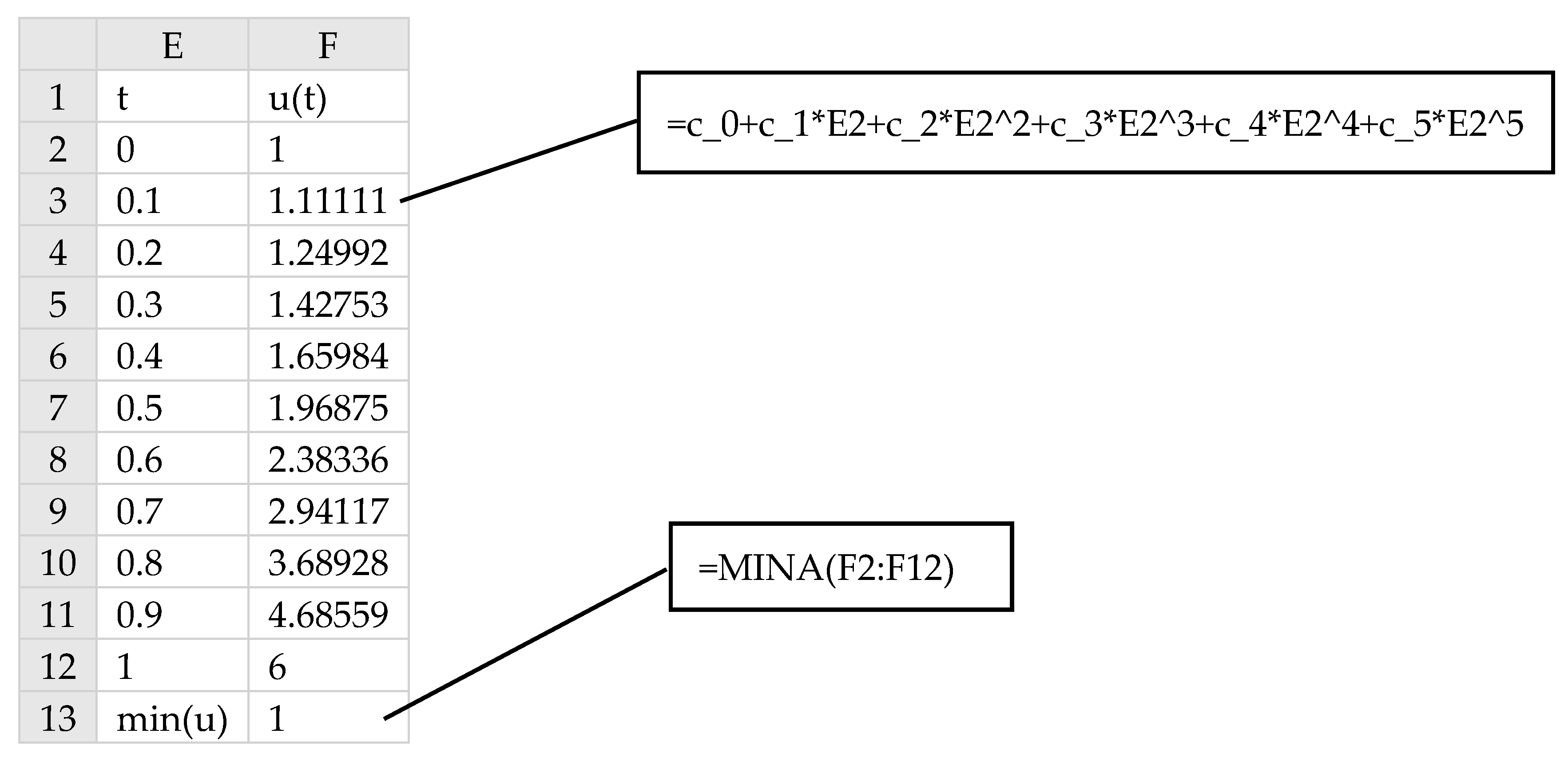
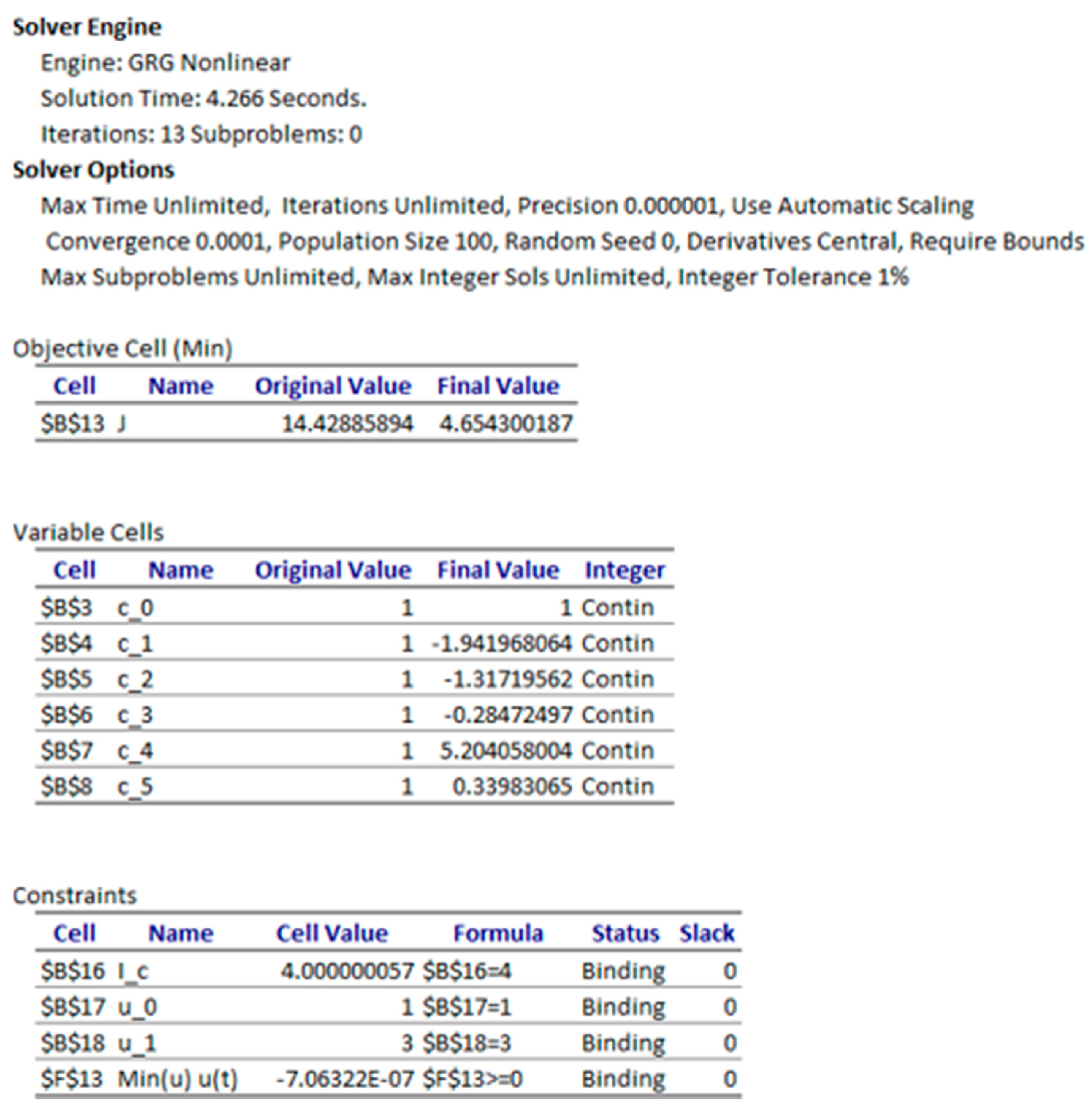
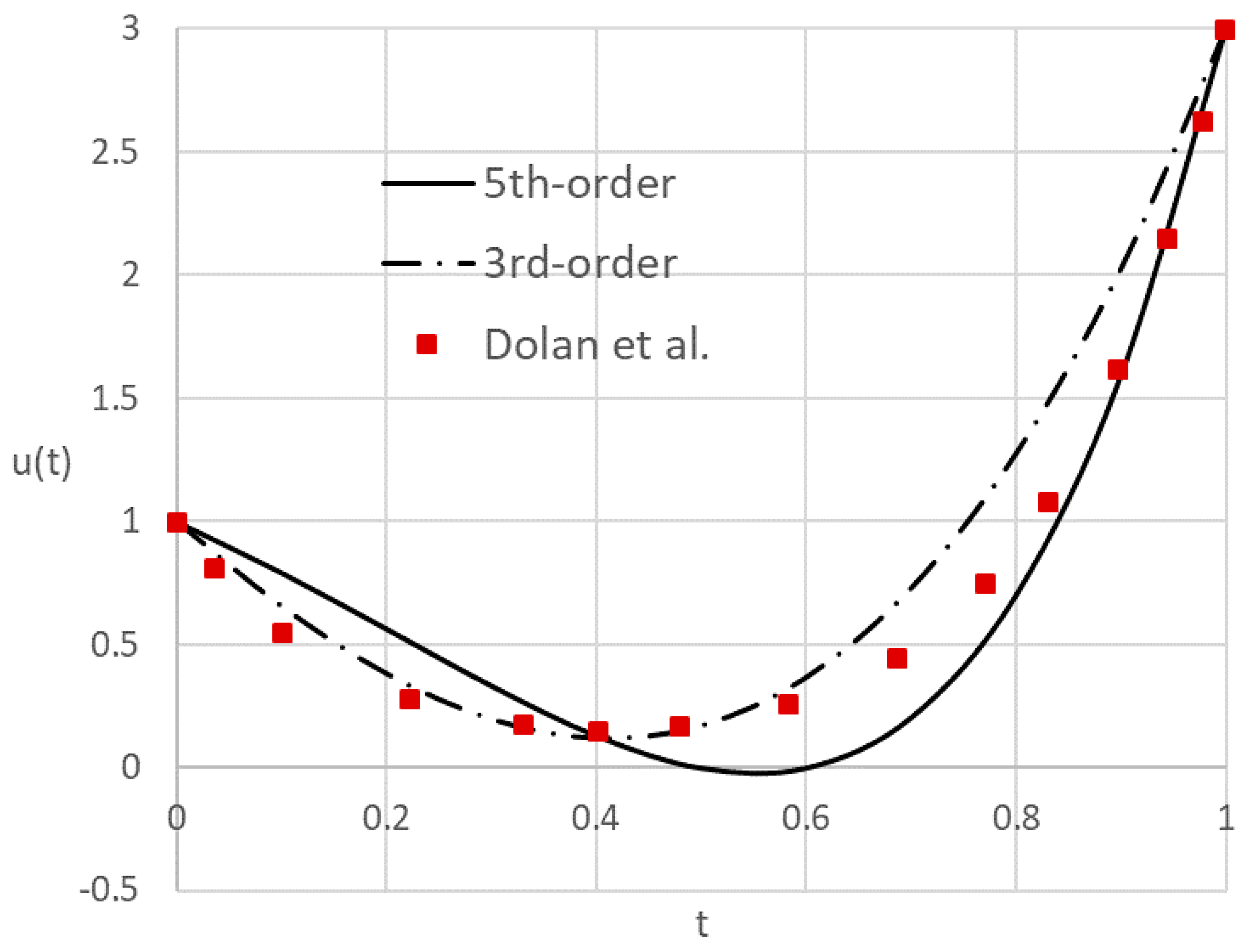
Incorporating (10) into the spreadsheet model was accomplished as follows. In a new column, a vector of time values from 0 to 1 in increment of 0.1 was generated using Excel AutoFill feature, along with a corresponding vector for the parametrized shape formula as shown in Figure 6. To impose (10), it is sufficient to demand that the minimum value of the shape vector, as computed in F13 of Figure 6, be greater than or equal to zero. Running the NLP solver with the added constraint yielded a cost index of 4.654 as shown in Figure 7 and plotted in Figure 8. The higher-order approximation to the shape function has resulted in a considerably lower cost index, by more than 8.3%, compared to that reported by Dolan et al. [19].
3.2. Quadratic Control Problem with Integral Constraint
The following problem which involves an integral dynamic constraint was studied by Lim et al. [20], who showed the that the optimal control can be calculated by solving an optimal parameter selection problem together with an unconstrained LQ problem. The optimal control problem is stated as follows:
Find which minimize the cost index
subject to
with initial conditions
and integral bounds constraint (There appears to be a typographical error in [20] where (15) is stated as less than 8. The actual value appears to be 80 since 8 would clearly violate the constraint at the reported optimal solution in [20].)
Lim et al. [20] calculated, with aid of control software MISER 3.1, an optimal cost index J of 62.66103.
3.2.1. Solution by Direct Spreadsheet Method
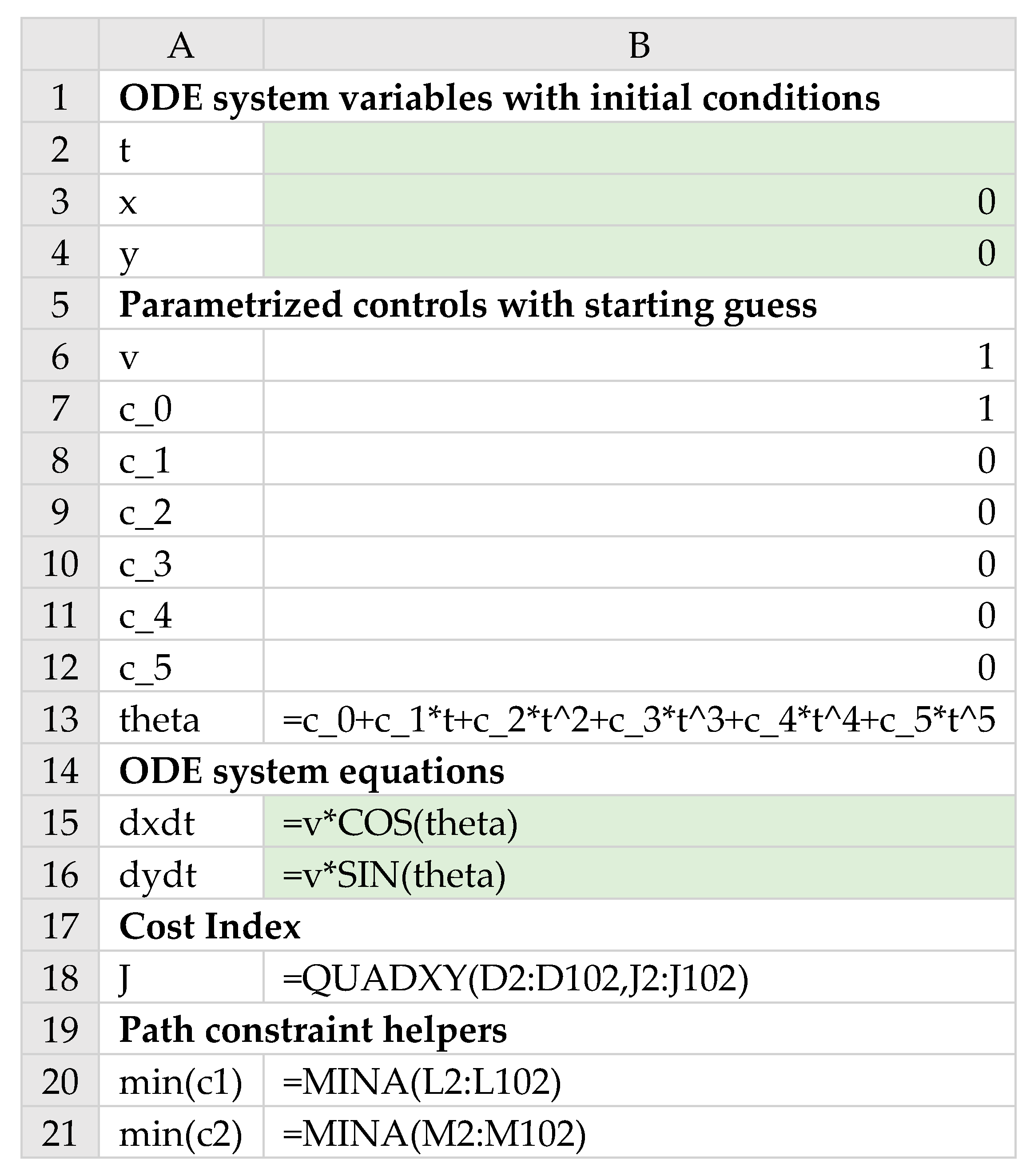
Referring to Figure 9 and working with named variables shown in column A, both and were parametrized using 3rd-order polynomials as shown in B10 and B11, and the IVP equations (12) and (13) were defined by equivalent formulas in B13 and B14. The state variables and are assigned the initial conditions as shown in B3 and B4. Next, an initial solution to the underlining IVP (12)–(14) was obtained by evaluating the formula
in an allocated array E1:G102. IVSOLVE was passed the IVP equations B13:B14, the IVP variables B2:B4, and the time interval [0, 1] and computed a formatted result shown partially in Figure 10. Here we have allocated 102 rows for the result array to display the solution at uniform time steps of 0.01.
=IVSOLVE(B13:B14, B2:B4, {0,1})
To define an equivalent formula for the cost index (11), we proceeded by sampling the controls formulas, and the cost index integrand as shown in columns I, J and K of Figure 10 by starting from the initial formulas shown in the figure and using AutoFill to generate the values. (Note the hierarchical interdependence of the generated columns on the IVP solution). Next, we defined the cost index formula in which the discrete data integrator calculus function QUADXY was employed to integrate the sampled integrand as shown in B16 of Figure 9. Similarly, we defined an analog formula for the integral constraint (15) as shown in B18 of Figure 9, and thus prepared all the input needed to run Excel NLP solver next.
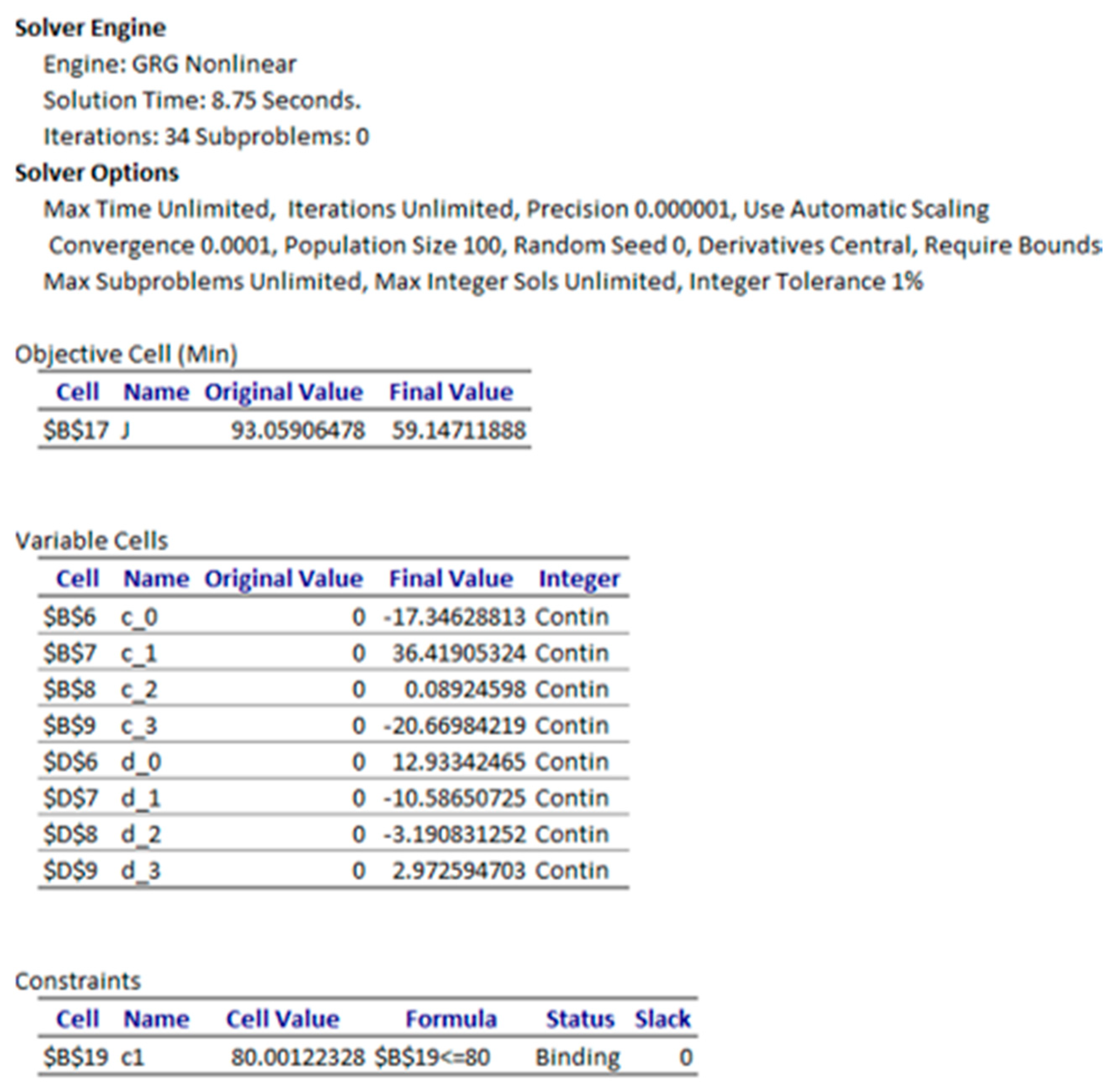
3.2.2. Results and Analysis
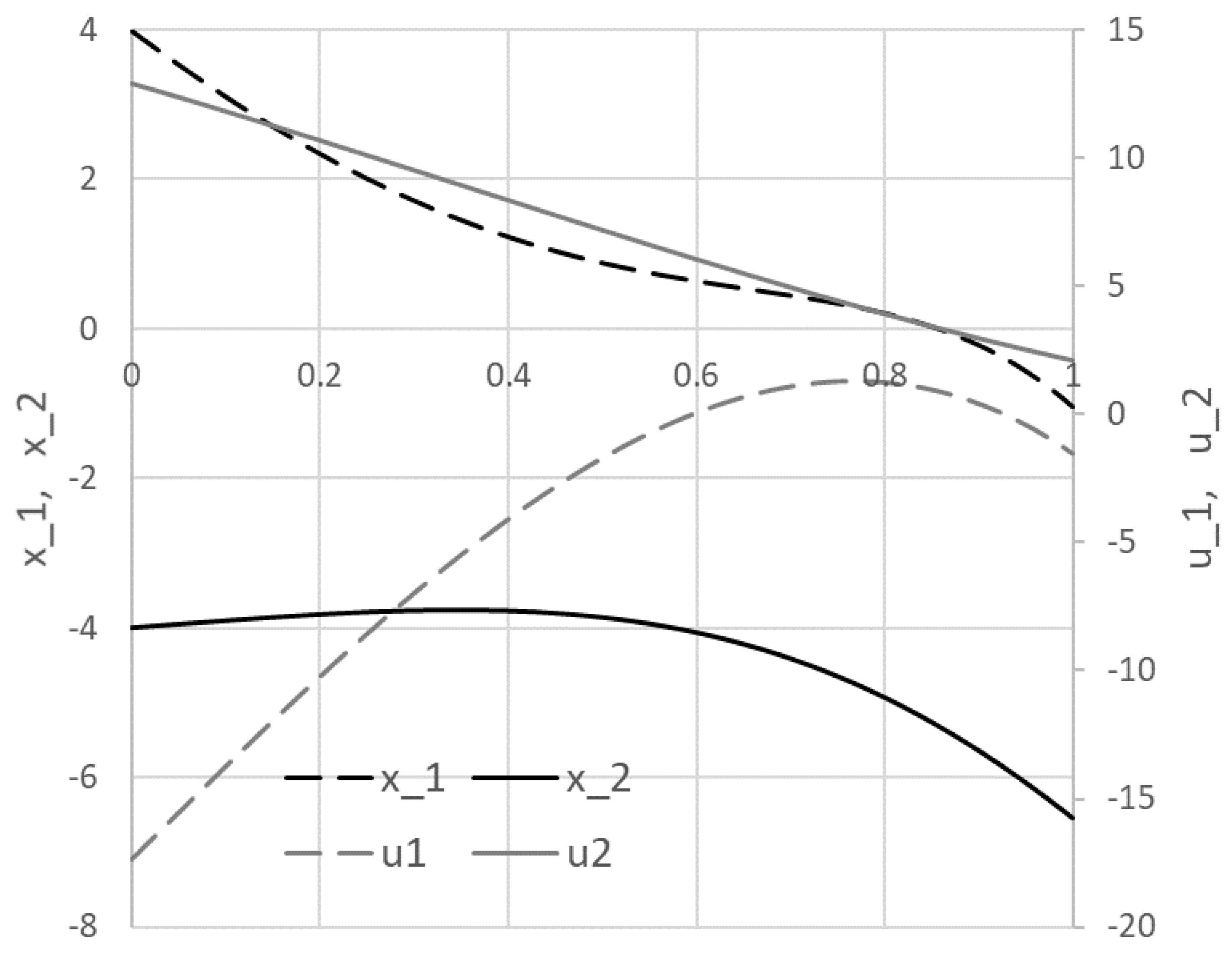
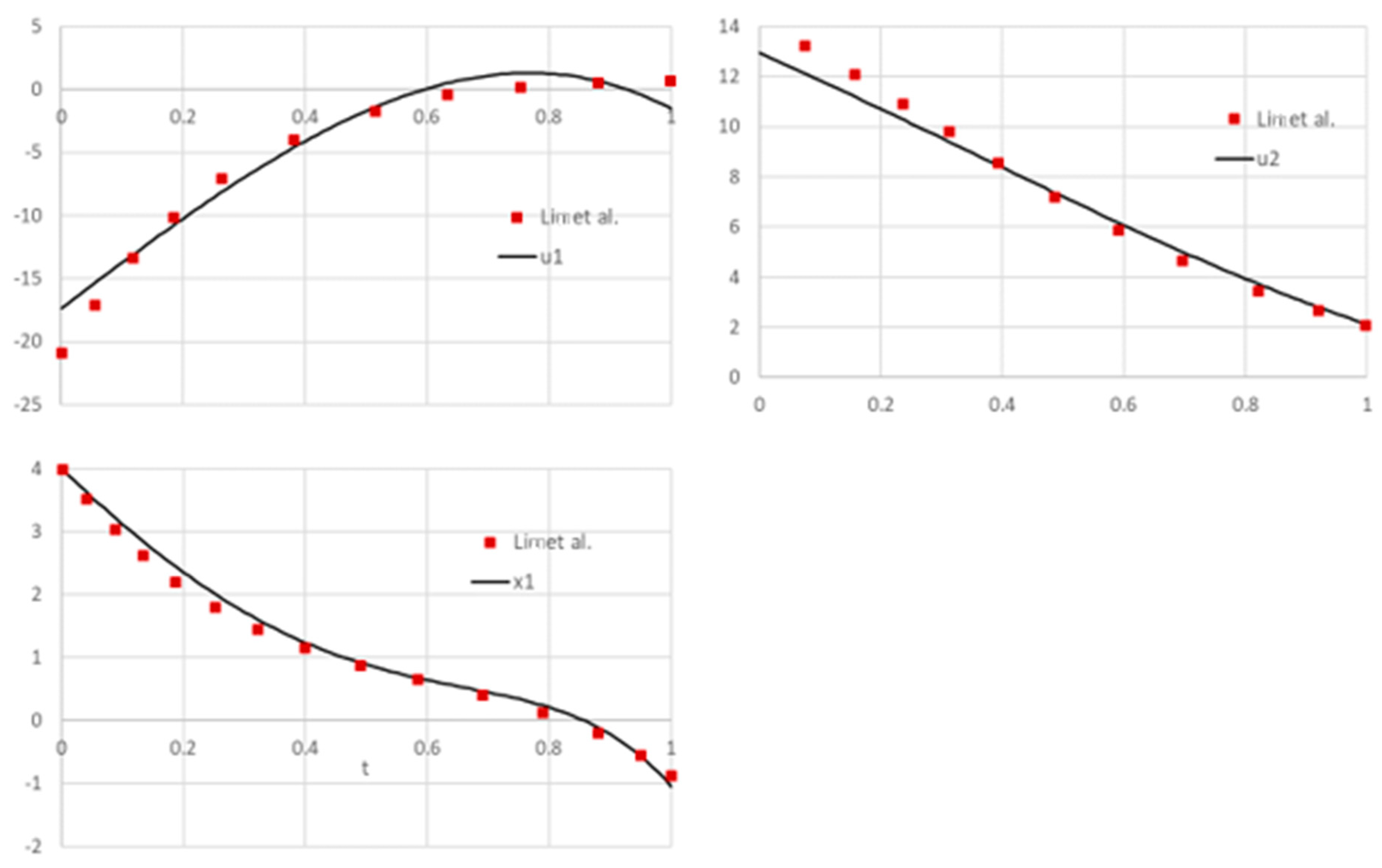
Excel solver was configured to minimize the cost index B16, by varying the controls coefficients B6:B9 and D6:D9, subject to the integral constraint B18 being smaller than or equal to 80. Excel solver converged in approximately eight seconds to the solution shown in Figure 11 and plotted in Figure 12. The obtained cost index at 59.1471 was lower than reported by Lim et al. [20] at 62.66103 using an indirect approach with MISER 3.1. Figure 13 provides direct comparisons for (t), and trajectories obtained by the current method and digitized plot values from [20]. The plots show good agreement despite fundamentally different solution strategies.
To investigate the effect of numerical integration error on the result, we increased the output array for IVSOLVE from 102 to 502 rows which reduced output time increment from 0.01 to 0.002. However, this has resulted in only minor improvement of the cost index to 59.1429, with otherwise insignificant change to the original solution which indicated the initial output time step of .01 was sufficient for accurate integration.
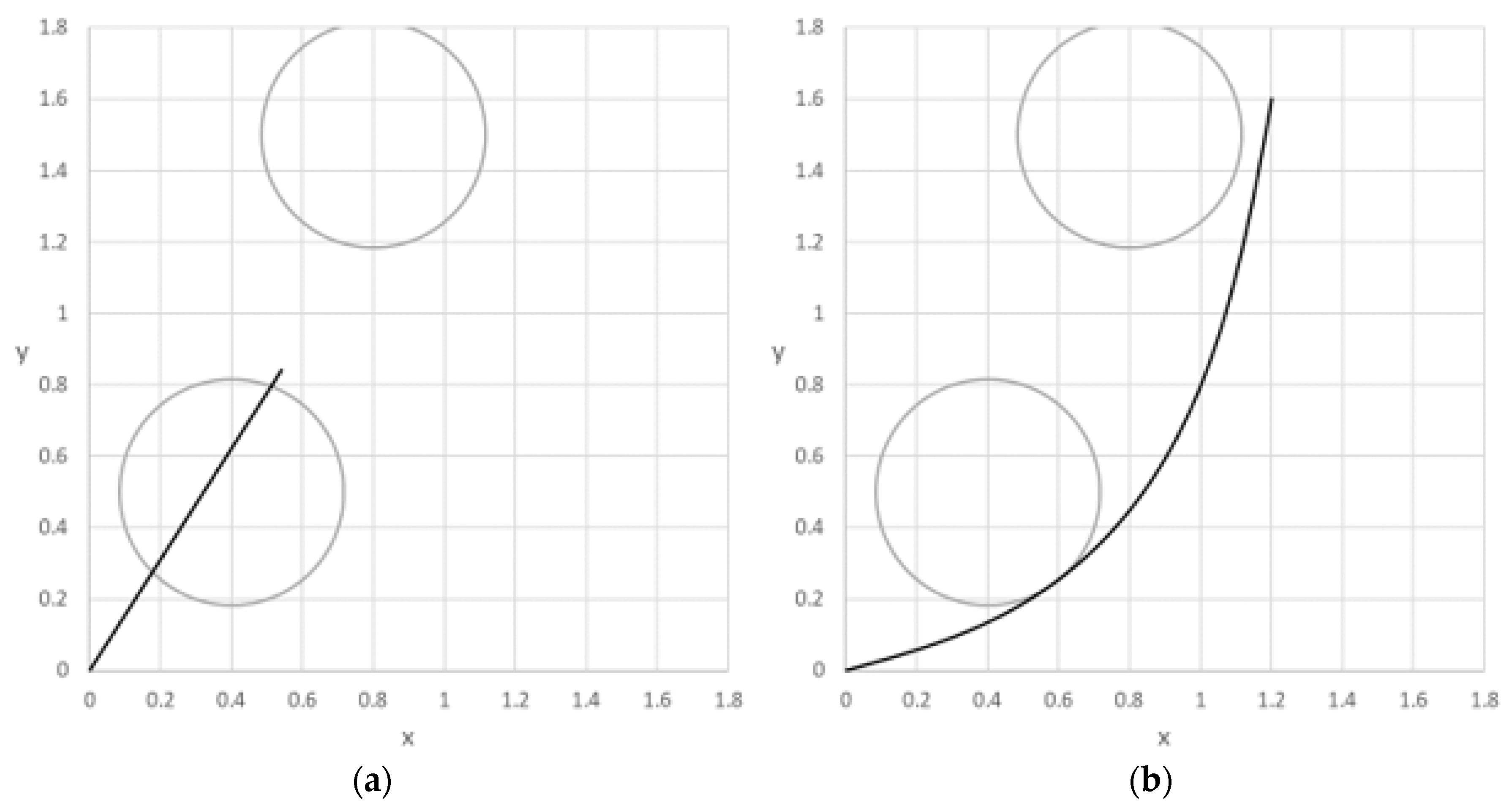
3.3. Robot Motion Planning: Obstacle Avoidance
The third problem is concerned with planning a 2D motion for a robot from point A (0, 0) to point B (1, 1), to avoid two circular obstacles of radius , centered at (0.4, 0.5) and (0.8, 1.5), while using the least amount of energy. The two controls for the robot motion are the constant speed, v, and the variable angle (direction), of the motion. The corresponding optimal control problem has the following form [21]:
Find which minimize the energy cost index
subject to
with initial conditions
end conditions
and trajectory constraints which model the circles to be avoided
Note that the cost index in this example depends on the second derivatives of the state variables.
3.3.1. Solution by Direct Spreadsheet Method
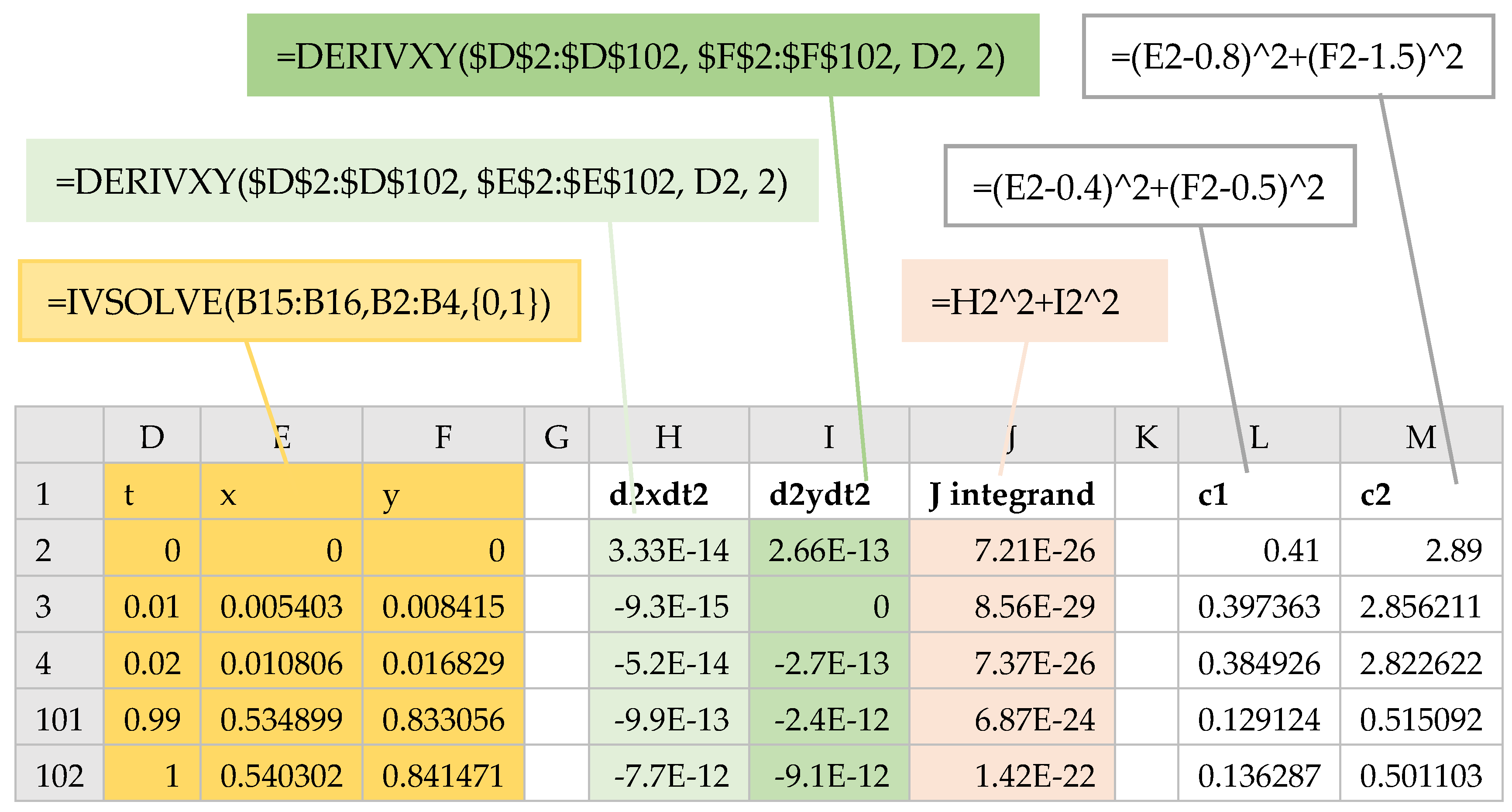
Referring to Figure 14, the speed was parametrized using the named variable v for B6 with initial value of 1, and the angle (named theta in B13) was parametrized with a fifth order polynomial. Using the named variable t, x and y, the IVP formulas (18) and (19) were defined in B15 and B16. An initial IVP solution was obtained by evaluating IVSOLVE formula (24) in array D1:F102 shown partially in Figure 15.
=IVSOLVE(B15:B16, B2:B4, {0,1})
The next task was to define an analog formula for the cost index (17). The integrand for the cost index depends on , and which we needed to generate. Although , and can be derived analytically for this particular problem by differentiating (18) and (19), we elected to compute them numerically using the discrete data differentiator calculus function DERIVXY as shown in columns H and I of Figure 15. For example, to compute , we started from the formula
in H2 passing in, respectively, the time and x vectors from the IVP solution array, the point of differentiation, and the order of the x derivative to compute. Next, the AutoFill was used to generate values for all the points in the time vector. Note that the first two arguments in (25) were locked using Excel $ operator to prevent these values from being incremented during the AutoFill, allowing only D2 to be incremented. Values for the integrand expression were then readily generated in a new column L and integrated with respect to the time vector by using the calculus function QUADXY as shown in B18 of Figure 14.
=DERIVXY($D$2:$D$102, $E$2:$E$102, D2, 2)
The remaining task to complete the input for Excel NLP solver was to define formulas for the circle avoidance constraints. Using x and y values from the IVP solution, values for the constraints equations (22) and (23) were generated as shown in columns L and M of Figure 15. To impose the bounds, it was sufficient to require that the minimum values of columns L and M, as computed in B20 and B21 of Figure 14, be greater than or equal to the specified bound.
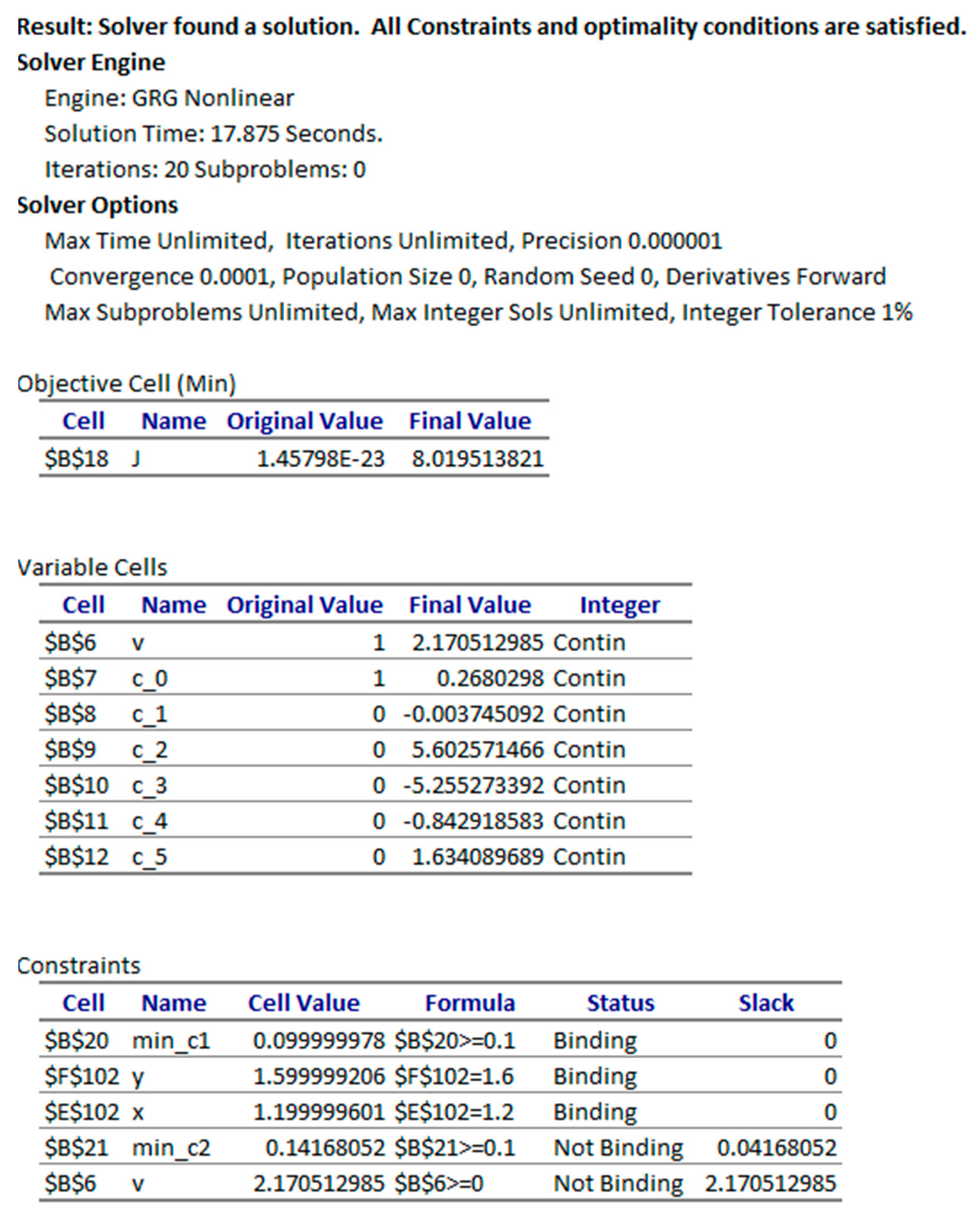
3.3.2. Results and Analysis
Excel solver was configured to minimize the cost index, J (B18), by varying the speed v (B6), and theta polynomial coefficients (B7:B12), subject to the constraints:
v >= 0,
E102 = 1.2, corresponding to (21)
F102 = 1.6, corresponding to (21)
B20 >= 0.1, corresponding to (22)
B21 >= 0.1, corresponding to (23).
The solver converged to the expected low-energy solution shown in Figure 16b in approximately 18 s, with the result shown in Figure 17. The initial trajectory for the robot based on our starting guess for the controls is shown in Figure 16a. The cost index was found at approximately 8.02.
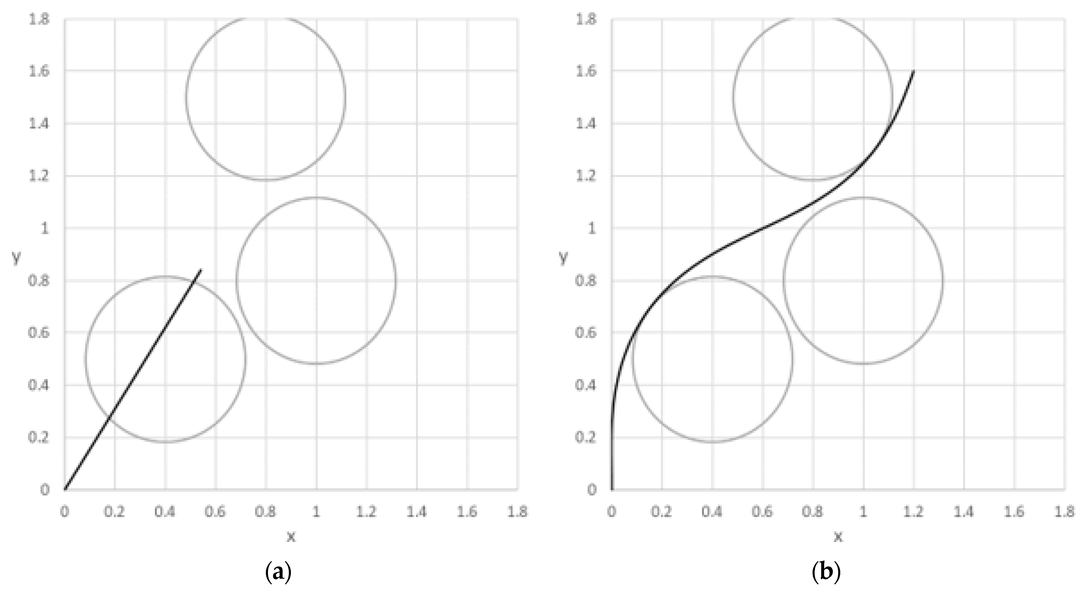
To make the problem more interesting, we added a 3rd circle obstacle by appending the additional path constraint to the problem:
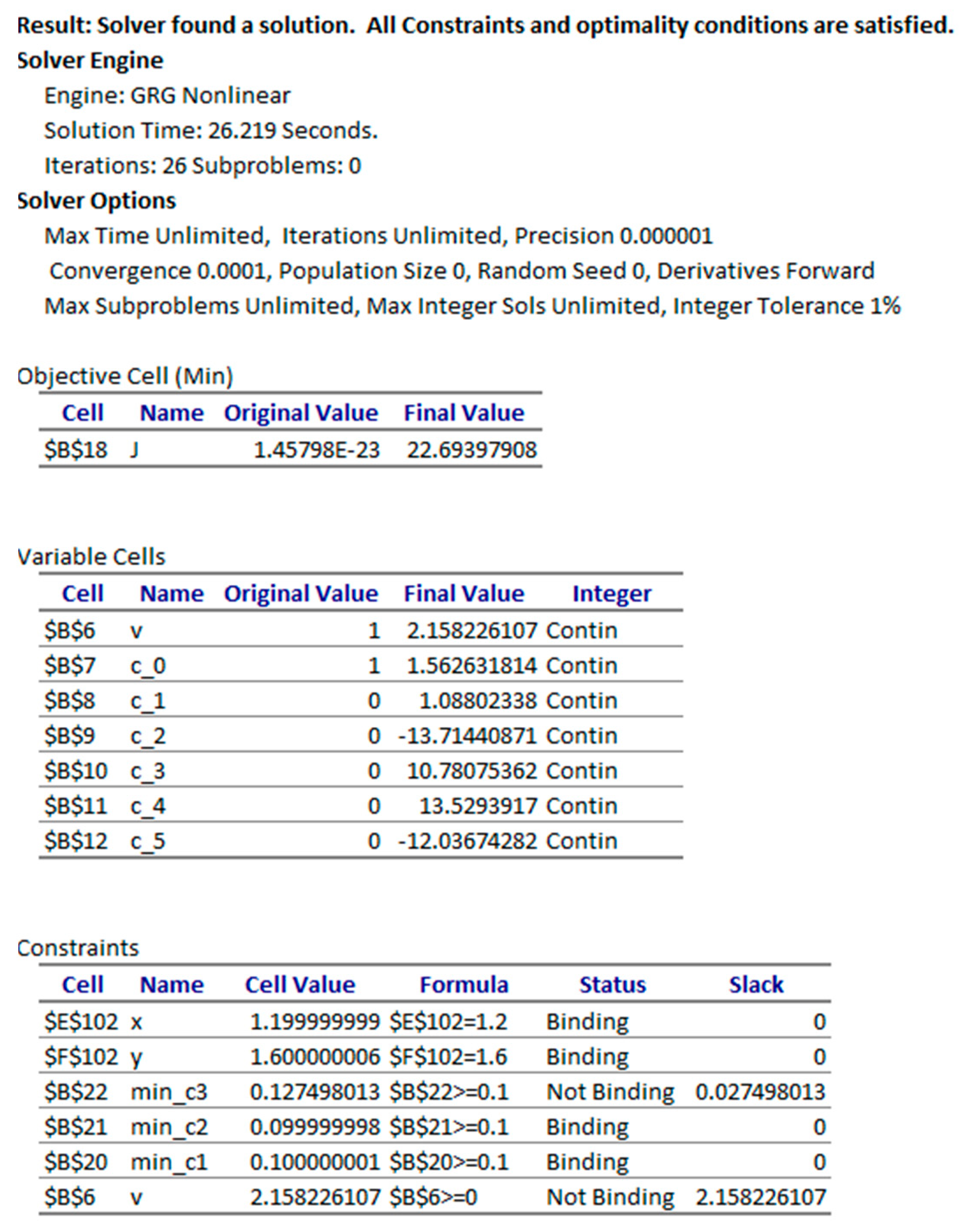
The new configuration and initial trajectory are shown in Figure 18a. The incorporation of the 3rd constraint into the model setup is straight forward and the solver converged to the higher energy trajectory shown in Figure 18b at a cost index of approximately 22.69; the results are shown in Figure 19.
3.4. Nonlinear Bioprocess Optimization: Batch Production
The 4th problem considers the optimal control of a fed-batch reactor for the production of ethanol [8]. The goal is to maximize the yield of ethanol using the feed rate as the control. This problem has highly nonlinear dynamic constraints and a free terminal time , which is also an unknown design variable. The mathematical statement of the free end time problem is given below:
Find the flowrate , and the terminal time to maximize the cost index
subject to
where
with Initial conditions
and bounds constraints
This problem was solved by Banga et al. [8] using a two-phase (stochastic-deterministic) hybrid (TPH) approach to overcome convergence difficulties reported by previous published attempts. Their best reported results found the maximum cost index J at 20839, and the terminal time at 61.17 h.
3.4.1. Solution by Direct Spreadsheet Method
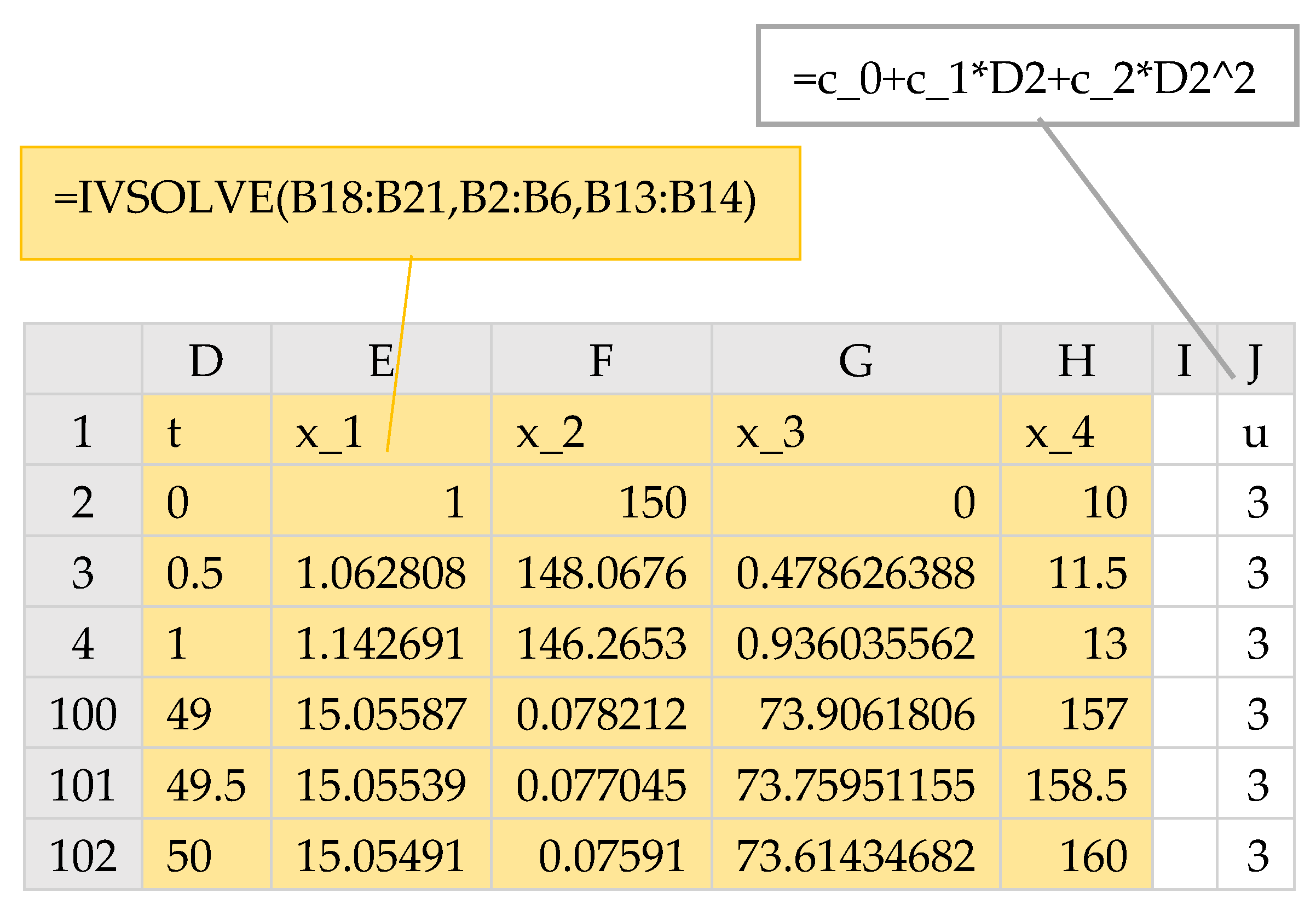
Following the procedure in the previous examples, the control u(t) was parameterized using a 2nd order polynomial as shown in B11 of Figure 20, and the IVP equations were defined in terms of the named variables as shown in B18:B21. Note that the terminal time has been assigned the variable B14 (named tF) with initial value of 50. The IVP solution was obtained with IVSOLVE formula
in array D1:H102 as shown partially in Figure 21. Note that the final time is now a variable for IVSOLVE which was passed in the 3rd parameter B13:B14. The cost index formula for this problem is simple and was defined by formula B23 which references and of the IVSOLVE solution array. To impose the bound constraint (35), we sampled the control formula in column J at the solution output time points as shown in Figure 21 and demanded that the maximum and minimum values of the control vector as computed by formulas B25 and B26 satisfy the appropriate bounds.
=IVSOLVE(B18:B21, B2:B6, B13:B14)
3.4.2. Results and Analysis
Excel solver was run starting from the initial guess for the unknown control coefficients and terminal time shown in Figure 20. The cost index J (B23) was selected to be maximized by varying the terminal time tF (B14), and the coefficients c_0, c_1 and c_2, (B8:B10) subject to the constraints:
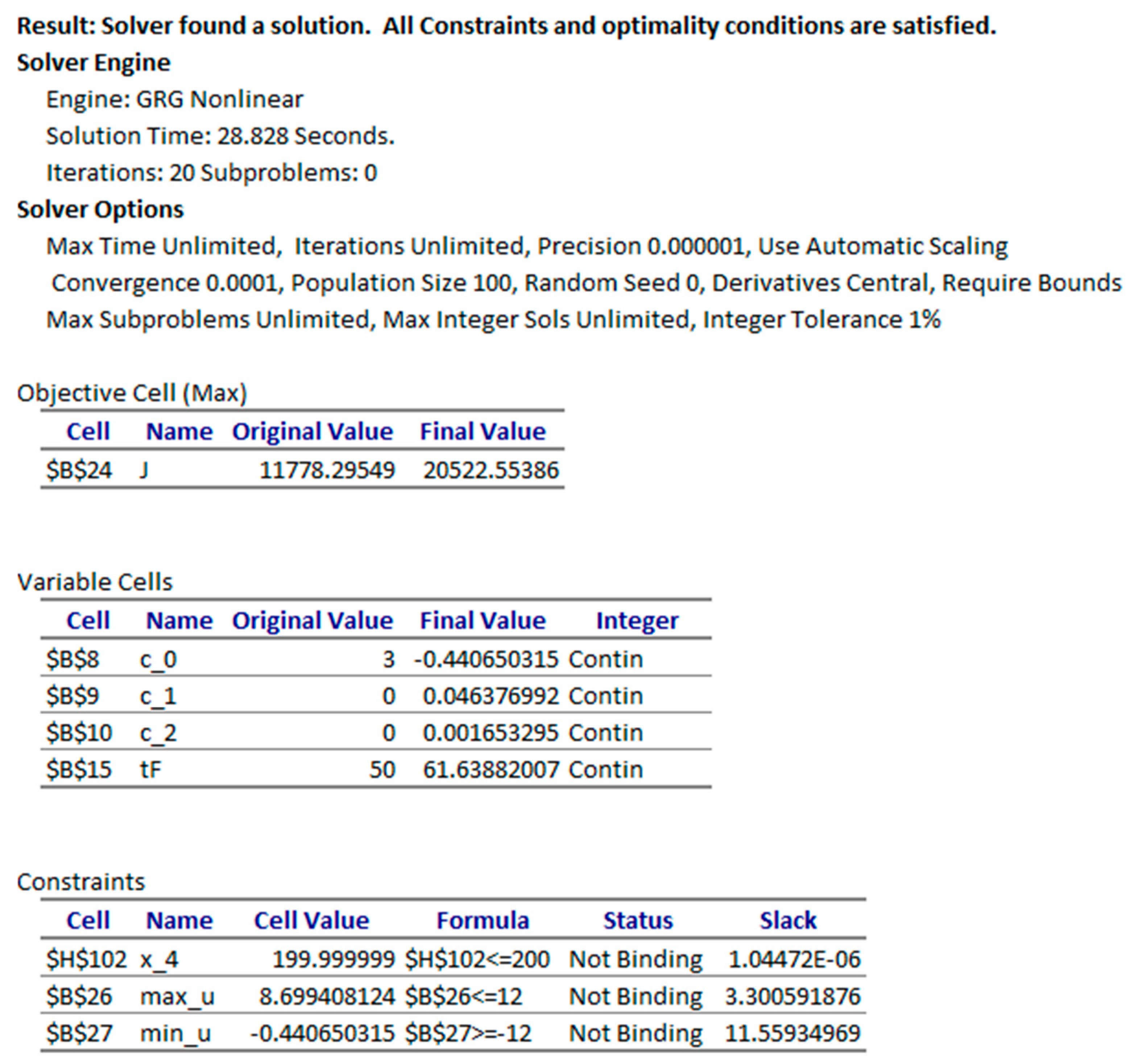
Excel NLP solver converged in approximately 29 s to the result shown in Figure 22, and plotted in Figure 23. A partial listing of the converged control values and IVP solution reflecting the new terminal time is shown in Figure 24.
B25 <= 12, corresponding to (35)
B26 >= −12, corresponding to (35)
H102 <= 200, corresponding to (36).
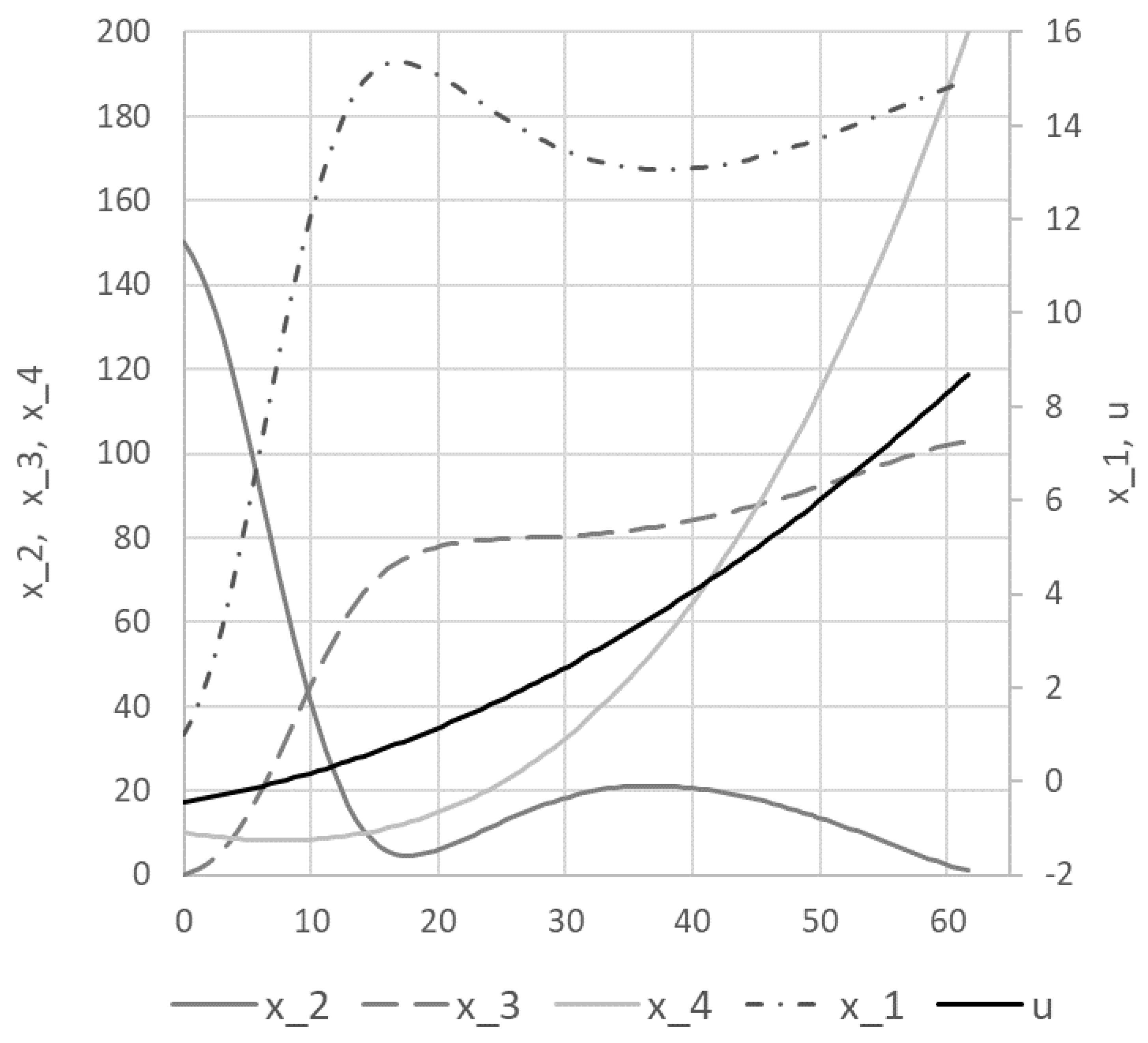
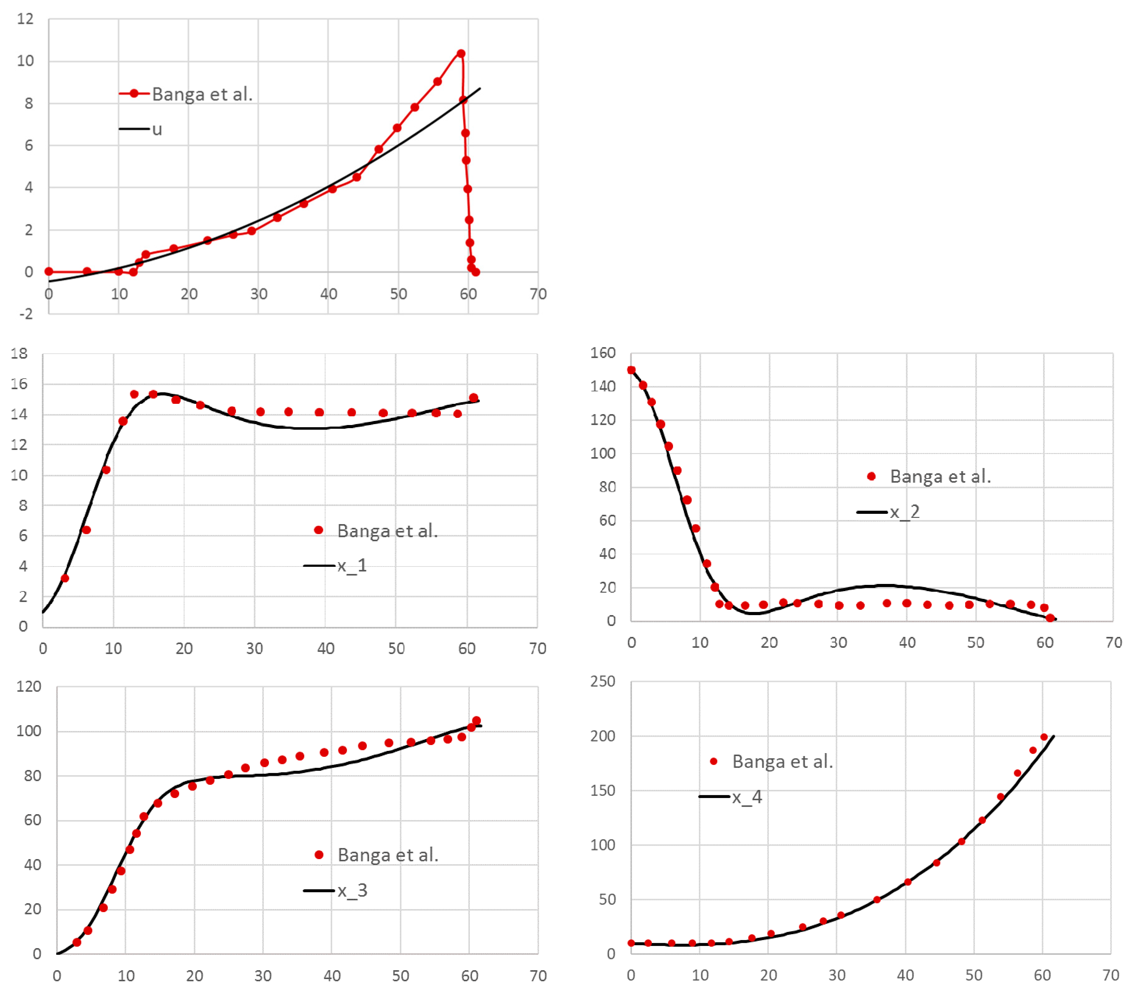
The achieved maxima for the cost index was at 20522.5 and the terminal time was found at approximately 61.64. These values are in very good agreement with the best results reported by Banga et al. [8] at 20839, and 61.17 h. Figure 25 shows direct comparison of the states and control trajectories with digitized plot values from Banga et al. The agreement is quite good for the most part despite fundamentally different control parametrization and algorithms employed by the two methods. In particular, the control parametrization in [8] is approximated by connected line segments, whereas our control is a continuous parabola.
4. Conclusions
We devised a practical and systematic spreadsheet solution strategy for solving general optimal control problems. The strategy is based on an adaptation of the partial-parametrization direct solution method which preserves the structure of the original mathematical optimization statement, but transforms it into a simplified NLP problem suitable for Excel NLP solver. The solution strategy is formulated by the aid of several elementary calculus functions from an available Excel calculus Add-in [11] for solving differential equations, computing integrals and derivatives. The calculus functions are employed as building blocks in a hierarchical functional paradigm implemented by standard Excel formulas in conjunction with Excel built-in NLP solver to carry out a dynamic optimization program.
Results were obtained for four representative problems selected to illustrate modeling of several conditions including dependence on higher order derivatives of state and controls as well as implicit IVP problems and integral constraints. The results were compared with published solutions obtained by other methods, and in some cases, were shown to be better by the measure of the cost index. The performance of the method is also notable with computing times on the order of seconds to a minute on a standard laptop. As has been illustrated by the solution procedure, applying the technique involves no more than defining a few formulas that parallel the original mathematical equations. No special programming skill is needed beyond basic familiarity with the common spreadsheet operation. The minimal problem setup effort, in combination with the ubiquity of Excel spreadsheet, present reasons to explore the method as an alternative, simpler educational tool for rather complex problems.
The success of the devised strategy for optimal control of ordinary differential equations supports future research for extending the strategy to optimal control of partial differential equations. In [22], the author demonstrated an analogous formulation combing the NLP solver with a PDE solver from the same Add-in [11] for parameter estimation of partial differential algebraic equations, and it may be feasible that certain formulations of optimal control of partial differential equations are solvable in the spreadsheet by a similar strategy. On the other hand, it is worth investigating devising an alternative strategy based on the indirect solution method [4,5] for optimal control problems. The indirect method requires solving a boundary value problem which could be solved by the aid of a boundary value problem solver function also available in the Excel calculus Add-in [11].
Supplementary Materials
An Excel workbook containing the solved problems in this paper is available online at https://www.mdpi.com/2297-8747/23/4/54/s1.
Funding
This research received no external funding.
Conflicts of Interest
The author of the manuscript is the founder of ExcelWorks LLC of Massachusetts, USA supplying the Excel calculus Add-in [11], utilized in this research work.
Appendix A
The following subsections present brief descriptions of the calculus functions utilized in this work. The functions are enabled as an extension of Excel math functions by installing ExceLab calculus Add-in [11]. For more detailed descriptions of the functions, the reader is referred to [11].
Appendix A.1. IVSOLVE: Initial Value Problem Solver
The worksheet function IVSOLVE solves an initial value differential algebraic equation system in the interval
, and M is an optional mass matrix which may be singular. IVSOLVE uses by default RADUA5 an implicit 5th-order Runge-Kutta scheme with adaptive time step [15], and at minimum, requires three input parameters to describe the ODE system:
- Reference to the right-hand side formulas corresponding to the vector-valued function .
- Reference to the system variables in the specific order ().
- The integration time interval end points.
Additional optional parameters include specifying a mass matrix as well as algorithmic controls. IVSOLVE is run as an array formula in an allocated array of cells. It evaluates to an ordered tabular result where the time values are listed in the first column, and the corresponding state variables’ values are listed in adjacent columns. By default, IVSOLVE reports the output at uniform intervals according to the allocated number of rows for the output array. Custom output formats can be achieved via the optional parameters including specifying custom divisions or exact points. We demonstrate IVSOLVE for the following DAE problem (reproduced from [14]):
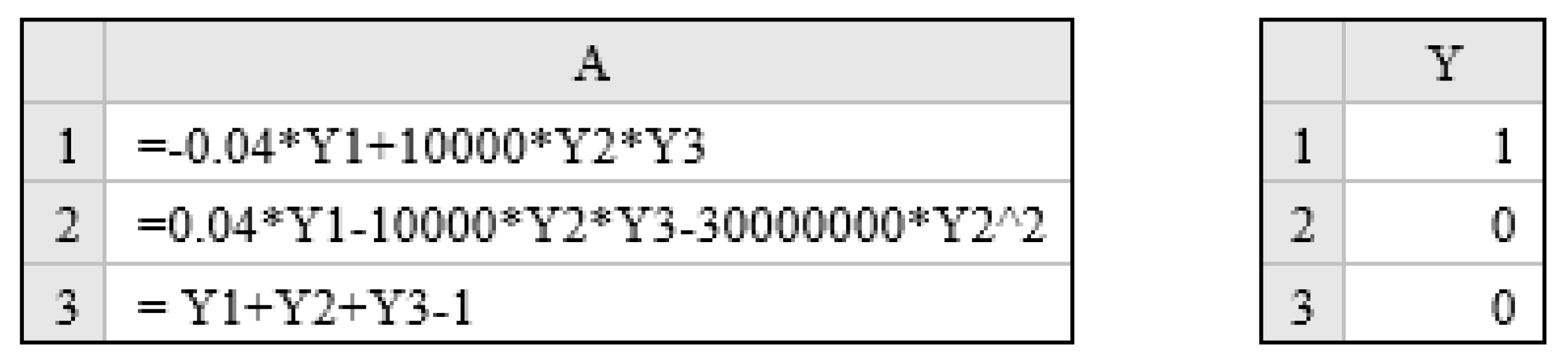
Referring to Figure A1, the system RHS formulas are defined in cells A1:A3 using cell T1 for the time variable and Y1, Y2, Y3 for the state variables which are assigned the initial conditions as shown in the figure.
Figure A1.
Spreadsheet model for equation system (A2).

To solve the system, we execute the array formula
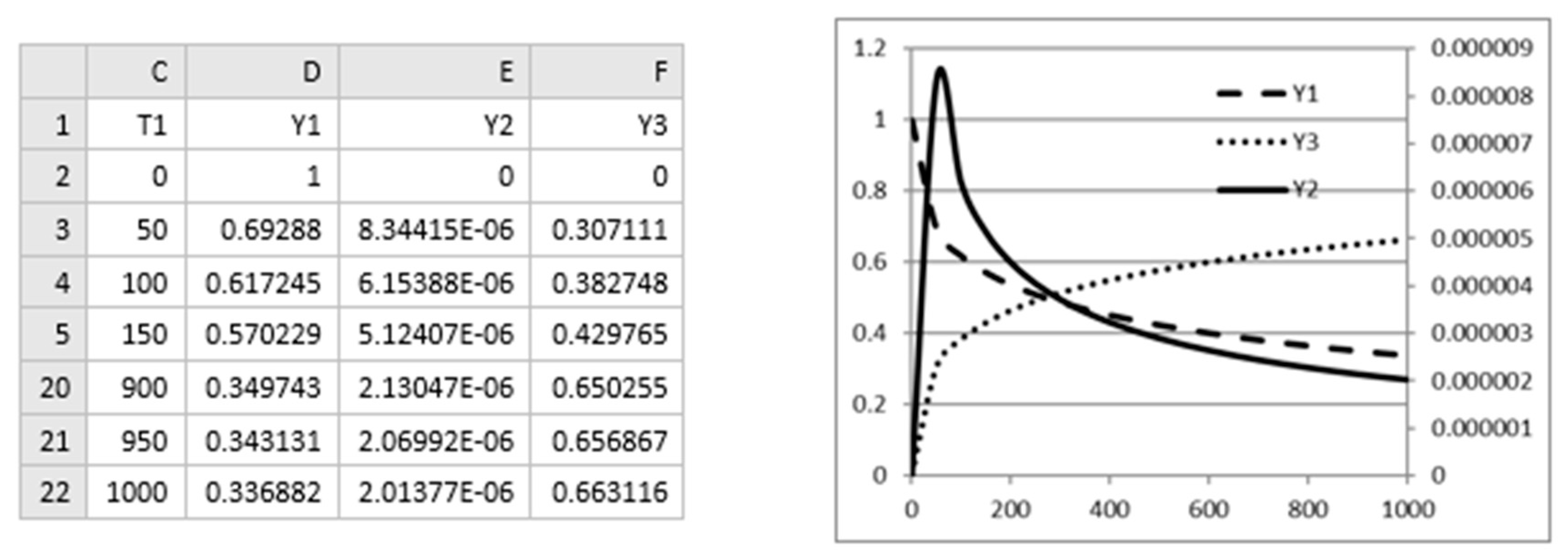
in an allocated array, (e.g., C1:F22) by pressing the 3 keys Control+Shift+Enter simultaneously. IVSOLVE computes and displays the solution shown Figure A2. Here we have used the 4th optional parameter to specify that the last equation, (A3) is an algebraic equation.
=IVSOLVE (A1:A3, (T1,Y1:Y3), {0,1000}, 1)
Figure A2.
Partial listing of the result computed by IVSOLVE (left) for system (A2), and a plot of the trajectories (right).
Figure A2.
Partial listing of the result computed by IVSOLVE (left) for system (A2), and a plot of the trajectories (right).

Appendix A.2. QUADF: Formula Integrator Function
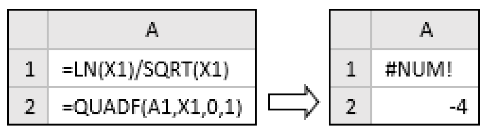
The spreadsheet function QUADF computes definite and improper one-dimensional integrals . QUADF utilizes QUADPACK numerical integration algorithms [17] suitable for smooth, irregular, and integrands with known singularities. By default, it uses QAG, an adaptive algorithm using Gauss-Kronrod 21-point integration rule. We demonstrate QUADF by computing the following integral (reproduced from [14]):
Referring to Figure A3, the integrand formula is defined in cell A1 using X1 as dummy variable for the integration. The QUADF integration formula
is defined in A2 passing in the integrand formula, the variable of integration, and values for the limits. Evaluating A2 yields the result.
=QUADF (A1, X1, 0, 1)
Figure A3.
Demonstration of QUADF for computing integral (A3) in Excel.

Using recursion, multiple integrals of any order can be computed by direct nesting of QUADF, as demonstrated by the following volume integral example:
To compute (A4), we construct a simple program consisting of three nested calls of QUADF as shown in Figure A4. Using X1, Y1 and Z1 as dummy variables, the integrand formula is defined in A1, and the inner, middle, and outer integrals formulas are defined in A2, A3 and A4 respectively, with each inner QUADF formula serving as the integrand for the next outer QUADF formula. Evaluating the outer integral in A4 computes the triple integral value.
Figure A4.
Demonstration of QUADF for computing multiple integral (A4) in Excel.

Appendix A.3. QUADXY: Discrete Data Integrator
The spreadsheet function QUADXY computes the integral of a curve passing through the set of data pairs . The integration interval is defined by the endpoints . QUADXY computes the integral by the aid of cubic (default) or linear splines fit to the data [16]. Start and end point slope information may be specified in the 3rd optional parameter to enhance accuracy near the end points. The slope data is defined by a reference to a key/value array as illustrated in Figure A5.
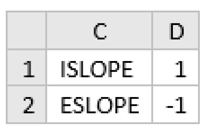
Figure A5.
Optional input format to QUADXY for endpoints boundary conditions.

For example, the formula
computes an integral value of 20 data pairs in columns X1 and Y1 with supplied optional end points slope values shown in Figure A5.
=QUADXY(X1:X20, Y1:Y20, C1:D2)
Appendix A.4. DERIVXY: Discrete Data Differentiator
The spreadsheet function DERIVXY employs cubic splines to compute the derivative of a curve passing through a set of data pairs at a specified point . Similar to QUADXY, optional start and or endpoint slope information may be specified to enhance accuracy near the end points. For example, the formula
computes the second derivative for a curve passing through 20 points in columns X1 and Y1 at the point x = 5.
=DERIVXY(X1:X20, Y1:Y20, 5, 2)
When using DERIVXY with Excel AutoFill feature to differentiate a given data set at multiple points, it is necessary to lock the parameters except for the variable point (parameter 3) so they are not incremented during the AutoFill. For example, the following formula is safe to use with AutoFill to generate derivatives at points stored in Z1, Z2, Z3, etc.
=DERIVXY($X$1:$X$20, $Y$1:$Y$20, Z1)
References
- Geering, H.P. Optimal Control with Engineering Applications; Springer: Berlin, Germany, 2007. [Google Scholar]
- Sethi, S.P. Optimal Control Theory: Applications to Management Science and Economics, 3rd ed.; Springer: Berlin, Germany, 2019. [Google Scholar]
- Aniţa, S.; Arnăutu, V.; Capasso, V. An Introduction to Optimal Control Problems in Life Sciences and Economics: From Mathematical Models to Numerical Simulation with MATLAB; Birkhäuser: Basel, Switzerland, 2011. [Google Scholar]
- Betts, J.T. Practical Methods for Optimal Control and Estimation Using Nonlinear Programming, 2nd ed.; Advances in Design and Control; Society for Industrial and Applied Mathematics: Philadelphia, PA, USA, 2009. [Google Scholar]
- Böhme, T.J.; Frank, B. Indirect Methods for Optimal Control. In Hybrid Systems, Optimal Control and Hybrid Vehicles. Advances in Industrial Control; Springer: Cham, Switzerland, 2017. [Google Scholar]
- Elnagar, G.; Kazemi, M.A. Pseudospectral Chebyshev Optimal Control of Constrained Nonlinear Dynamical Systems. Comput. Optim. Appl. 1998, 11, 195–217. [Google Scholar] [CrossRef]
- Böhme, T.J.; Frank, B. Direct Methods for Optimal Control. In Hybrid Systems, Optimal Control and Hybrid Vehicles. Advances in Industrial Control; Springer: Cham, Switzerland, 2017. [Google Scholar]
- Banga, J.R.; Balsa-Canto, E.; Moles, C.G.; Alonso, A.A. Dynamic optimization of bioprocesses: Efficient and robust numerical strategies. J. Biotechnol. 2003, 117, 407–419. [Google Scholar] [CrossRef] [PubMed]
- Rodrigues, H.S.; Torres Monteiro, M.T.; Torres, D.F.M. Optimal Control and Numerical Software: An Overview. arXiv, 2014; arXiv:1401.7279. [Google Scholar]
- Ghaddar, C.K. Novel Spreadsheet Direct Method for Optimal Control Problems. Math. Comput. Appl. 2018, 23, 6. [Google Scholar] [CrossRef]
- ExcelWorks LLC, MA, USA. ExceLab Calculus Add-in and Reference Manual. Available online: https://excel-works.com (accessed on 22 September 2018).
- Nævdal, E. Solving Continuous Time Optimal Control Problems with a Spreadsheet. J. Econ. Educ. 2003, 34, 2. [Google Scholar] [CrossRef]
- Weber, E.J. Optimal Control Theory for Undergraduates Using the Microsoft Excel Solver Tool. Comput. High. Educ. Econ. Rev. 2007, 19, 4–15. [Google Scholar]
- Ghaddar, C. Unconventional Calculus Spreadsheet Functions. World Academy of Science, Engineering and Technology, International Science Index 112. Int. J. Math. Comput. Phys. Electr. Comput. Eng. 2016, 10, 194–200. [Google Scholar]
- Hairer, E.; Wanner, G. Solving Ordinary Differential Equations II: Stiff and Differential-Algebraic Problems; Springer Series in Computational Mathematics; Springer: Berlin, Germany, 1996. [Google Scholar]
- De Boor, C. A Practical Guide to Splines (Applied Mathematical Sciences); Springer: Berlin, Germany, 2001. [Google Scholar]
- Piessens, R.; de Doncker-Kapenga, E.; Ueberhuber, C.W.; Kahaner, D.K. Quadpack: A Subroutine Package for Automatic Integration; Springer: Berlin, Germany, 1983. [Google Scholar]
- Lasdon, L.S.; Waren, A.D.; Jain, A.; Ratner, M. Design and Testing of a Generalized Reduced Gradient Code for Nonlinear Programming. ACM Trans. Math. Softw. 1978, 4, 34–50. [Google Scholar] [CrossRef] [Green Version]
- Dolan, E.D.; More, J.J. Benchmarking Optimization Software with Cops; Technical Report; Argonne National Laboratory: Argonne, IL, USA, 2001. [Google Scholar]
- Lim, A.E.B.; Liu, Y.Q.; Teo, K.L.; B, M.J. Linear-quadratic optimal control with integral quadratic constraints. Optim. Control Appl. Methods 1999, 20, 79–92. [Google Scholar] [CrossRef]
- Bhattacharya, R. OPTRAGEN 2.0: A MATLAB Toolbox for Optimal Trajectory Generation; Texas A & M University: College Station, TX, USA, 2013. [Google Scholar]
- Ghaddar, C.K. Rapid Modeling and Parameter Estimation of Partial Differential Algebraic Equations by a Functional Spreadsheet Paradigm. Math. Comput. Appl. 2018, 23, 39. [Google Scholar] [CrossRef]
Figure 1.
Illustration of the ordered steps to define an analog formula for the cost index (1) which encapsulates the inner IVP (2)–(3).
Figure 1.
Illustration of the ordered steps to define an analog formula for the cost index (1) which encapsulates the inner IVP (2)–(3).

Figure 2.
Spreadsheet parametrized model for problem 3.1.

Figure 3.
Input to Excel solver for problem 3.1 based on the spreadsheet model in Figure 2.
Figure 3.
Input to Excel solver for problem 3.1 based on the spreadsheet model in Figure 2.

Figure 4.
Answer report generated by Excel solver using 3rd order parametrization for problem 3.1.

Figure 5.
Optimal u(t) computed using 3rd order parametrization for problem 3.1. Reported values by Dolan et al. are also shown.
Figure 5.
Optimal u(t) computed using 3rd order parametrization for problem 3.1. Reported values by Dolan et al. are also shown.

Figure 6.
Parametrized u(t) function is sampled with AutoFill to provide a handle on its minimum value for the purpose of imposing constraint (10).
Figure 6.
Parametrized u(t) function is sampled with AutoFill to provide a handle on its minimum value for the purpose of imposing constraint (10).

Figure 7.
Answer report generated by Excel solver using a 5th order parametrization for problem 3.1 with the added constrained (10).
Figure 7.
Answer report generated by Excel solver using a 5th order parametrization for problem 3.1 with the added constrained (10).

Figure 8.
Optimal u(t) computed by using 5th order parametrization for problem 3.1. The higher-cost solution with 3rd order parametrization and reported values by Dolan et al. are also shown.
Figure 8.
Optimal u(t) computed by using 5th order parametrization for problem 3.1. The higher-cost solution with 3rd order parametrization and reported values by Dolan et al. are also shown.

Figure 9.
Spreadsheet parametrized model for problem 3.2. The colored ranges are inputs for IVSOLVE formula (16).
Figure 9.
Spreadsheet parametrized model for problem 3.2. The colored ranges are inputs for IVSOLVE formula (16).

Figure 10.
Partial display of IVP (12)–(14) solution obtained by IVSOLVE formula (16), and dependent generated columns for the parametrized controls formulas, and the integrand expression for the cost index (11).
Figure 10.
Partial display of IVP (12)–(14) solution obtained by IVSOLVE formula (16), and dependent generated columns for the parametrized controls formulas, and the integrand expression for the cost index (11).

Figure 11.
Answer report generated by Excel solver for problem 3.2.

Figure 12.
Optimal trajectories computed by the spreadsheet method for problem 3.2.

Figure 13.
Direct comparison of spreadsheet solution with reported solution obtained by Lim et al. [20] for problem 3.2.
Figure 13.
Direct comparison of spreadsheet solution with reported solution obtained by Lim et al. [20] for problem 3.2.

Figure 14.
Spreadsheet parametrized model for problem 3.3. The colored ranges are inputs for IVSOLVE formula (24).
Figure 14.
Spreadsheet parametrized model for problem 3.3. The colored ranges are inputs for IVSOLVE formula (24).

Figure 15.
Partial display of the IVP (18)–(20) solution obtained by IVSOLVE formula (24), and dependent generated values needed to define the cost index and constraints formulas of problem 3.3.
Figure 15.
Partial display of the IVP (18)–(20) solution obtained by IVSOLVE formula (24), and dependent generated values needed to define the cost index and constraints formulas of problem 3.3.

Figure 16.
Initial (a) and optimal (b) trajectories for problem 3.3.

Figure 17.
Answer report generated by Excel Solver for problem 3.3.

Figure 18.
Initial (a) and optimal (b) trajectories for problem 3.3 with additional constraint (26).
Figure 18.
Initial (a) and optimal (b) trajectories for problem 3.3 with additional constraint (26).

Figure 19.
Answer report generated by Excel Solver for problem 3.3 with additional constraint (26).

Figure 20.
Spreadsheet parametrized model for problem 3.4. The colored ranges are inputs for IVSOLVE formula (37).
Figure 20.
Spreadsheet parametrized model for problem 3.4. The colored ranges are inputs for IVSOLVE formula (37).

Figure 21.
Partial display of IVP (28)–(34) solution obtained by IVSOLVE formula (37), and generated values for the parametrized control of problem 3.4.
Figure 21.
Partial display of IVP (28)–(34) solution obtained by IVSOLVE formula (37), and generated values for the parametrized control of problem 3.4.

Figure 22.
Answer report generated by Excel solver for problem 3.4.

Figure 23.
Optimal trajectories computed by the spreadsheet method for problem 3.4.

Figure 24.
Partial listing of the converged IVP solution and control values of problem 3.4.

Figure 25.
Direct comparison of spreadsheet solution with reported solution obtained by Banga et al. for problem 3.4.
Figure 25.
Direct comparison of spreadsheet solution with reported solution obtained by Banga et al. for problem 3.4.

© 2018 by the author. Licensee MDPI, Basel, Switzerland. This article is an open access article distributed under the terms and conditions of the Creative Commons Attribution (CC BY) license (http://creativecommons.org/licenses/by/4.0/).
Share and Cite
MDPI and ACS Style
Ghaddar, C.K. Rapid Solution of Optimal Control Problems by a Functional Spreadsheet Paradigm: A Practical Method for the Non-Programmer. Math. Comput. Appl. 2018, 23, 54. https://doi.org/10.3390/mca23040054
AMA Style
Ghaddar CK. Rapid Solution of Optimal Control Problems by a Functional Spreadsheet Paradigm: A Practical Method for the Non-Programmer. Mathematical and Computational Applications. 2018; 23(4):54. https://doi.org/10.3390/mca23040054
Chicago/Turabian StyleGhaddar, Chahid Kamel. 2018. "Rapid Solution of Optimal Control Problems by a Functional Spreadsheet Paradigm: A Practical Method for the Non-Programmer" Mathematical and Computational Applications 23, no. 4: 54. https://doi.org/10.3390/mca23040054