Time Needed to Control an Epidemic with Restricted Resources in SIR Model with Short-Term Controlled Population: A Fixed Point Method for a Free Isoperimetric Optimal Control Problem

Abstract

In this paper, we attempt to determine the optimal duration of an anti-epidemic control strategy which targets susceptible people, under the isoperimetric condition that we could not control all individuals of this category due to restricted health resources. We state and prove the local and global stability conditions of free and endemic equilibria of a simple epidemic compartmental model devised in the form of four ordinary differential equations which describe the dynamics of susceptible-controlled-infected-removed populations and where it is taken into account that the controlled people cannot acquire long-lived immunity to move towards the removed compartment due to the temporary effect of the control parameter. Thereafter, we characterize the sought optimal control and we show the effectiveness of this limited control policy along with the research of the optimal duration that is needed to reduce the size of the infected population. The isoperimetric constraint is defined over a fixed horizon, while the objective function is defined over a free horizon present under a quadratic form in the payoff term. The complexity of this optimal control problem requires the execution of three numerical methods all combined together at the same time, namely, the forward–backward sweep method to generate the optimal state and control functions, the secant method adapted to the isoperimetric restriction, and, finally, the fixed point method to obtain the optimal final time.

1. Introduction

1.1. Background

Many epidemiological models have been interested in the study of the dynamics of susceptible, infected and removed individuals who belong to a sample of a population threatened by an infection. Many theoretical models in epidemiology have been devised to show the effect of different anti-epidemic control strategies when they are followed to prevent transmission of a particular type of infection to the susceptible population. As examples of these control approaches, we can cite Refs. [1,2] where the authors introduced an awareness control function in their models and which aimed to prevent the susceptible people from Human Immunodeficiency Virus infection and Acquired Immune Deficiency Syndrome (HIV/AIDS) epidemic. Roy et al. [3] treated the idea of awareness control programs in HIV/AIDS prevention after the addition of a new variable in their models and which defines the number of individuals in the aware class. Other examples of control models have used vaccination of the susceptible individuals as a control policy, while considering the number of vaccinated people as additional compartment in their systems (see [3,4,5,6,7]). Most optimal control strategies suggested for preventing an infection to spread consider a fixed final time. However, health policy-makers need very often to know when it is appropriate to stop their anti-epidemic measures as this information is important for managing their medical resources [8], and then, it becomes not reasonable in such situations to study dynamics of an epidemic under control without an estimation of the final time. The present paper tries to find the optimal value of this mentioned variable through a free horizon optimal control approach applied to an epidemic model with four compartments, namely classes of susceptible, controlled, infected and removed people.

1.2. Formulation of the Problem of Interest for this Investigation

Here, we devise a simple generalized model where the control utilized has only a temporary effect on the immunity of the targeted population so the susceptible people under control do not acquire long-lived immunity to move to the removed class, while taking into account the presence of an equation which describes the evolution of the number of the controlled people. First, we study the local and global stability of our epidemic model, which is devised in the form of four ordinary differential equations, and wherein a control is introduced as a constant parameter; and, second, we seek the optimal duration needed for reaching the goal of our strategy while determining the optimal value of this control when it is changed to a function of time under the hypothesis that this anti-epidemic preventive measure can reach only a specific fraction of susceptible people due to the limited health resources. We should note that authors of [8,9] tried to find the optimal final time in a first case through their plots and checked the values where this optimal function verified the obtained additional necessary condition, and in two other cases via discrete numerical schemes. We believe this work is more interesting, as it provides a more precise numerical method. In fact, as the necessary condition on final time also represents here a fixed point equation, the incorporation of the fixed point method better facilitates our task, as this technique seems more accurate and convincing since it meets the theoretical aspect of the found condition.

1.3. Literature Survey

Zhou and Fan [10] discussed different forms of functions introduced in epidemic models to explore the impact of limited medical resources in the transmission of infectious diseases. Abdelrazec et al. [11] introduced, in a mathematical model of dengue fever, a function in place of the recovery rate for similar purpose. More recently, Yu et al. proposed an optimal control approach to investigate the optimal distribution policy of the limited vaccination resources based on the research of a parameter introduced in their model and which minimizes the basic reproduction number [12].

1.4. Scope and Contribution of this Study

We present here an optimal control approach which treats the problem of limited resources differently to the three above-mentioned references. In fact, our method considers a constraint, so-called “isoperimetric”, which is used on the control function as done in [13] for the resolution of a dosage problem, on the fraction of controlled variables as done in [14] in the case of an epidemic model, or when adapted to a discrete-time SIRS epidemic model as in [15], and it supposes also that the final time or horizon of the objective function is free (non-fixed) as used in many applications (see, for example, Ref. [8], which discusses the problem of optimal duration needed for reaching the intravesical therapy goal, and Ref. [9], where it is explained why such considerations are very important to health-policy makers and managers in the health sector when there is an epidemic that is controlled through awareness of the susceptible class).

1.5. Organization of the Paper

Based on the theory of mathematical epidemiology in [16], the spread of an epidemic can be described mathematically by SIR models which in turn have been developed later to extended forms such as SEIR [17], SIRS [18], or SIS [19], where each letter refers to a class of individuals. A class of controlled people can also be considered, as done in [20] where authors added a vaccination compartment in a model of pertussis and tuberculosis, and in [21] where they studied nonfatal diseases, and [22,23] in case of influenza. Sharomi and Malik [24] represented an other form of SIR model with an additional equation corresponding to the vaccinated category in the case the vaccination is not $100\%$ effective; such considerations can also be found in [4]. Based on similar assumptions as in the two last mentioned references, we devise our present model.

In the following parts of the paper, we start with the presentation of our mathematical model and study its stability in cases of free and endemic equilibria. Furthermore, we seek the optimal value of the free horizon considered in the objective function, along with the determination of the optimal value of the control function. Finally, we discuss our numerical results.

2. The Mathematical Model and Stability

In this section, we consider a mathematical model with the four following main compartments:

• S is the number of susceptible people to infection or who are not yet infected.
• $C_S$ is the number of susceptible people who are temporarily controlled so they cannot move to the removed class due to the limited effect of control.
• I is the number of infected people who are capable of spreading the epidemic to those in the susceptible and temporary controlled categories.
• R is the number of removed people from the epidemic.

In our modeling approach, we choose to describe dynamics of variables S, $C_S$, I and R at time t, based on the following differential system

$$\left\{\begin{array}{ccc}\dot{S}\left(t\right)\hfill & =\hfill & \mathsf{\Pi }\left(t\right)-\beta S\left(t\right)I\left(t\right)-a\theta S\left(t\right)-\mu S\left(t\right)\hfill \\ \dot{C_S}\left(t\right)\hfill & =\hfill & a\theta S\left(t\right)-b\beta C_S\left(t\right)I\left(t\right)-\mu C_S\left(t\right)\hfill \\ \dot{I}\left(t\right)\hfill & =\hfill & \beta (S\left(t\right)+b{C}_S\left(t\right))I\left(t\right)-\gamma I\left(t\right)-\mu I\left(t\right)\hfill \\ \dot{R}\left(t\right)\hfill & =\hfill & \gamma I\left(t\right)-\mu R\left(t\right)\hfill \end{array}\right.$$

(1)

with initial conditions $S\left(0\right)>0$, $C_S\left(0\right)\ge 0$, $I\left(0\right)\ge 0$ and $R\left(0\right)\ge 0$, and where $\mathsf{\Pi }\left(t\right)=\mu N\left(t\right)$, with $N\left(t\right)=S\left(t\right)+C_S\left(t\right)+I\left(t\right)+R\left(t\right)$ as the total population size, gives the newborn people at time t; $a\theta$$(0\le a\le 1)$ is the recruitment rate of susceptibles to the controlled class with $\theta$ defining the control parameter as a constant between 0 and 1 and “a” modeling the reduced chances of a susceptible individuals to be controlled; $\beta ={\displaystyle \frac{\delta }{N\left(t\right)}}$ with $\delta$ the infection transmission rate, $\mu$ the natural death rate, $b\theta$$(0\le b\le 1)$ the recruitment rate of controlled people to the infected class even in the presence of $\theta$ and “b” modeling the reduced chances of a temporarily controlled individual to be infected; and $\gamma$ is the recovery rate. We note that the population size is constant because $\dot{N}\left(t\right)=\dot{S}\left(t\right)+{\dot{C}}_S\left(t\right)+\dot{I}\left(t\right)+\dot{R}\left(t\right)=0$. Hence, $N\left(t\right)=N=aconstant$, and then, $\mathsf{\Pi }\left(t\right)=\mathsf{\Pi }=aconstant$.

For the sake of readability, hereafter, we use S, $C_S$, I and R as notations of the time functions $S\left(t\right)$, $C_S\left(t\right)$, $I\left(t\right)$ and $R\left(t\right)$.

Recalling that ${\displaystyle R_0=\frac{\beta }{\mu +\gamma }}$ is the basic reproduction number of the standard SIR model (see [25] where it is concluded that the disease free equilibrium $E^0$ is global asymptotically stable if $R_0\le 1$, and there exists a global asymptotically stable and unique endemic equilibrium $E^{+}$ if $R_0>1$).

Since the two first equations are independent of the last equation, we only study the stability of the following differential system

$$\left\{\begin{array}{ccc}\dot{S}\hfill & =\hfill & \mathsf{\Pi }-\beta SI-a\theta S-\mu S\hfill \\ \dot{C_S}\hfill & =\hfill & a\theta S-b\beta C_{S}I-\mu C_S\hfill \\ \dot{I}\hfill & =\hfill & \beta (S+b{C}_S)I-\gamma I-\mu I\hfill \end{array}\right.$$

(2)

A disease free equilibrium in our case can be defined as $E^0=(S^0,C_S^0,0)$ where $S^0$ and $C_S^0$ are obtained based on the assumptions $\dot{S}=0$ and $\dot{I}=0$ when there is no infection.

Explicitly, we have $\dot{S}=0$ when $I=0$, gives ${\displaystyle S^0=\frac{\mathsf{\Pi }}{\mu +a\theta }}$. In addition, we have $\dot{C_S}=0$ when $I=0$, gives ${\displaystyle C_S^0=\frac{a\theta \mathsf{\Pi }}{\mu (\mu +a\theta )}}$.

If ${lim}_{t\to +\infty }{C}_S\left(t\right)=0$ as a consequence of the case when $\theta =0$, we define the basic reproduction number for our case by $R_0^C$ which is the average new infections produced by one infected individual during his life cycle when the population is at $E^0$.

Since I is the only infected compartment, then ${\displaystyle R_0^C=\beta (S^0+b{C}_S^0)\times \frac{1}{\mu +\gamma }}$. Thus, we have

$${\displaystyle R_0^C=\frac{\beta \mathsf{\Pi }}{(\mu +a\theta )(\mu +\gamma )}+\frac{ab\beta \theta \mathsf{\Pi }}{\mu (\mu +a\theta )(\mu +\gamma )}=\frac{\beta \mathsf{\Pi }(\mu +ab\theta )}{\mu (\mu +a\theta )(\mu +\gamma )}}$$

(3)

Now, we try to find the components of the endemic equilibrium $E^{+}=(S^{+},C_S^{+},I^{+})$ where $S^{+}$ and $C_S^{+}$ are obtained based on the assumptions $\dot{S}=0$ and $\dot{C_S}=0$ when there is an infection.

Explicitly, we have $\dot{S}=0$ when $I>0$, which gives ${\displaystyle S^{+}=\frac{\mathsf{\Pi }}{\mu +a\theta +\beta I^{+}}}$. In addition, we have $\dot{C_S}=0$ when $I>0$, which gives ${\displaystyle C_S^{+}=\frac{a\theta S^{+}}{\mu +b\beta I^{+}}}$.

On the other part, we have $\dot{I}=0$ when $I>0$, which gives

$$\begin{array}{c}\beta S^{+}{I}^{+}+b\beta C_S^{+}{I}^{+}-\gamma I^{+}-\mu I^{+}=0\hfill \\ {\displaystyle \Rightarrow \beta \frac{\mathsf{\Pi }}{\mu +a\theta +\beta I^{+}}+\beta \frac{ab\theta S^{+}}{\mu +b\beta I^{+}}=\gamma +\mu }\hfill \\ \Rightarrow \beta \mathsf{\Pi }(\mu +b\beta I^{+})+ab\beta \theta S^{+}(\mu +a\theta +\beta I^{+})=(\gamma +\mu )(\mu +a\theta +\beta I^{+})(\mu +b\beta I^{+})\hfill \\ \Rightarrow \beta \mathsf{\Pi }(\mu +b\beta I^{+})+ab\beta \theta \mathsf{\Pi }=(\gamma +\mu )(\mu +a\theta +\beta I^{+})(\mu +b\beta I^{+})\hfill \\ \Rightarrow b{\beta }^2\mathsf{\Pi }{I}^{+}+\beta \mathsf{\Pi }(\mu +ab\theta )=(\gamma +\mu )(\mu +a\theta +\beta I^{+})(\mu +b\beta I^{+})\hfill \\ \Rightarrow (\gamma +\mu )(\mu +a\theta )R_0^C\mu -(\gamma +\mu )(a\theta \mu +{\mu }^2)\hfill \\ =b{\beta }^2(\gamma +\mu )I^{{+}^2}+[(\gamma +\mu )(\beta \mu (1+b)+ab\beta \theta )-b{\beta }^2\mathsf{\Pi }]I^{+}\hfill \end{array}$$

Thus, we find that $I^{+}$ is the root of the function $f\left(I^{+}\right)={\alpha }_1{I}^{{+}^2}+{\alpha }_2{I}^{+}+(1-R_0^C){\alpha }_3$ where ${\alpha }_1,{\alpha }_2$ and ${\alpha }_3$ are constants.

In the following three theorems, we state and prove stability results on free and endemic equilibria.

Theorem 1.

$E^0$ always exists and is locally asymptotically stable if $R_0^C<1$ (respectively, $E^0$ is unstable if $R_0^C>1$).

Proof. 

The existence of $E^0$ is trivial.

For the stability of $E^0$, we define the Jacobian Matrix associated to the system in Equation (2) by

$$\begin{array}{c}\hfill \left(\begin{array}{ccc}-\beta I-a\theta -\mu & 0& -\beta S\\ a\theta & -b\beta I-\mu & -b\beta C_S\\ \beta I& b\beta I& \beta (S+b{C}_S)-\gamma -\mu \end{array}\right)\end{array}$$

(4)

At $E^0$, (4) becomes

$$\begin{array}{c}\hfill \left(\begin{array}{ccc}-a\theta -\mu & 0& -\beta S^0\\ a\theta & -\mu & -b\beta C_S^0\\ 0& 0& \beta (S^0+b{C}_S^0)-\gamma -\mu \end{array}\right)\end{array}$$

whose eigenvalues are

$$\begin{array}{c}{\lambda }_1=-\mu <0,\hfill \\ {\lambda }_2=-(\mu +a\theta )<0\hfill \\ {\lambda }_3=\beta (S^0+b\beta C_S^0)-\gamma -\mu =(\gamma +\mu )(R_0^C-1),\hfill \end{array}$$

which imply the local asymptotic stability of $E^0$ when $R_0^C<1$, and its instability when $R_0^C>1$. □

Theorem 2.

The differential system in Equation (2) admits $E^{+}=\left({\displaystyle \frac{\mathsf{\Pi }}{\mu +a\theta +\beta I^{+}},\frac{a\theta S^{+}}{\mu +b\beta I^{+}},I^{+}}\right)$ as the unique positive equilibrium and which is asymptotically stable when it exists, if and only if $R_0^C>1$.

Proof. 

First, we have

$$\begin{array}{c}{\alpha }_1=b{\beta }^2(\gamma +\mu )>0,\hfill \\ {\alpha }_2=[(\gamma +\mu )(\beta \mu (1+b)+ab\beta \theta )-b{\beta }^2\mathsf{\Pi }],\hfill \\ {\alpha }_3=\mu (\gamma +\mu )(\mu +a\theta )>0\hfill \end{array}$$

For the sufficiency of the existence and uniqueness of $E^{+}$, so we have ${\alpha }_1>0$ and since $f\left(0\right)=(1-R_0^C){\alpha }_3<0$ if $R_0^C>1$, then $f\left(I^{+}\right)$ has two real roots, one is positive and the other is negative. For the necessity, let us assume that $R_0^C\le 1$ and prove that $f\left(I^{+}\right)$ has no positive roots. In this case, the first fraction in Equation (3) verifies

$$\begin{array}{c}\beta \mathsf{\Pi }\le (\mu +\gamma )(\mu +a\theta )\hfill \\ \Rightarrow {\alpha }_2=(b\beta (\mu +a\theta )+\mu \beta )(\gamma +\mu )-b{\beta }^2\mathsf{\Pi }\hfill \\ \ge \left(b\beta \right(\mu +a\theta )+\mu \beta )(\gamma +\mu )-b\beta (\mu +a\theta )(\mu +\gamma )=\mu \beta (\gamma +\mu )>0.\hfill \end{array}$$

Thus, we have ${\alpha }_1>0$ and since $f\left(0\right)=(1-R_0^C){\alpha }_3\ge 0$, $f\left(I^{+}\right)$ is increasing and $f\left(I^{+}\right)>f\left(0\right)\ge 0$, then we reach the non-positivity of the roots.

For the stability of $E^{+}$, at $E^{+}$, Equation (4) is defined as

$$\begin{array}{c}\hfill \left(\begin{array}{ccc}-\beta I^{+}-a\theta -\mu & 0& -\beta S^{+}\\ a\theta & -b\beta I^{+}-\mu & -b\beta C_S^{+}\\ \beta I^{+}& b\beta I^{+}& \beta (S^{+}+b{C}_S^{+})-\gamma -\mu \end{array}\right)\end{array}$$

$$\begin{array}{c}\hfill =\left(\begin{array}{ccc}{\displaystyle -\frac{\mathsf{\Pi }}{S^{+}}}& 0& -\beta S^{+}\\ a\theta & {\displaystyle -\frac{a\theta S^{+}}{C_S^{+}}}& -b\beta C_S^{+}\\ \beta I^{+}& b\beta I^{+}& 0\end{array}\right)\end{array}$$

whose characteristic equation is ${\lambda }^3+{\sigma }_1{\lambda }^2+{\sigma }_2\lambda +{\sigma }_3$ and where

$$\begin{array}{c}{\displaystyle {\sigma }_1=\frac{\mathsf{\Pi }}{S^{+}}+\frac{a\theta S^{+}}{C_S^{+}}}\hfill \\ {\displaystyle {\sigma }_2=\frac{a\theta \mathsf{\Pi }}{C_S^{+}}+b^2{\beta }^2{C}_S^{+}{I}^{+}+{\beta }^2{S}^{+}{I}^{+}}\hfill \\ {\displaystyle {\sigma }_3=ab{\beta }^2\theta S^{+}{I}^{+}+\frac{a\theta {\beta }^2{S}^{{+}^2}{I}^{+}}{C_S^{+}}+\frac{b^2{\beta }^2\mathsf{\Pi }{C}_S^{+}{I}^{+}}{S^{+}}.}\hfill \end{array}$$

Hence, we have

$$\begin{array}{c}{\sigma }_1{\sigma }_2-{\sigma }_3\hfill \\ {\displaystyle =\frac{\mathsf{\Pi }}{S^{+}}\left({\displaystyle \frac{a\theta \mathsf{\Pi }}{C_S^{+}}+{\beta }^2{S}^{+}{I}^{+}}\right)}\hfill \\ {\displaystyle +\frac{a\theta S^{+}}{C_S^{+}}\left({\displaystyle \frac{a\theta \mathsf{\Pi }}{C_S^{+}}+b^2{\beta }^2{C}_S^{+}{I}^{+}}\right)-ab{\beta }^2\theta S^{+}{I}^{+}}\hfill \\ {\displaystyle =\frac{a\theta {\mathsf{\Pi }}^2}{S^{+}{C}_S^{+}}+(\mathsf{\Pi }+a\theta +\beta I^{+}){\beta }^2{S}^{+}{I}^{+}}\hfill \\ {\displaystyle +\frac{a\theta S^{+}}{C_S^{+}}\left({\displaystyle \frac{a\theta \mathsf{\Pi }}{C_S^{+}}+b^2{\beta }^2{C}_S^{+}{I}^{+}}\right)-ab{\beta }^2\theta S^{+}{I}^{+}}\hfill \\ {\displaystyle =\frac{a\theta {\mathsf{\Pi }}^2}{S^{+}{C}_S^{+}}+(\mathsf{\Pi }+\beta I^{+}){\beta }^2{S}^{+}{I}^{+}+\frac{a^2{\theta }^2\mathsf{\Pi }{S}^{+}}{C_S^{{+}^2}}}\hfill \\ +a\theta S^{+}{I}^{+}{(\beta -b\beta )}^2+ab{\beta }^2\theta S^{+}{I}^{+}\hfill \\ >0\hfill \end{array}$$

Finally, based on the Routh–Hurwitz Criterion, we deduce the local asymptotic stability of $E^{+}$. □

Theorem 3.

If $R_0^C\le 1$, then $E^0$ is globally asymptotically stable. If $R_0^C>1$, then $E^{+}$ is globally asymptotically stable.

Proof. 

We suppose that $R_0^C\le 1$ and we prove that $E^0$ is globally asymptotically stable. Let us define the Lyapunov function by

$${\displaystyle L_0=S-S^0-S^{0}ln\frac{S}{S^0}+C_S-C_S^0-C_S^{0}ln\frac{C_S}{C_S^0}+I.}$$

Its derivative is then defined by

$$\begin{array}{c}{\displaystyle \dot{L_0}=\dot{S}+\dot{C_S}+\dot{I}-S^0\frac{\dot{S}}{S}-C_S^0\frac{\dot{C_S}}{C_S}}\hfill \\ {\displaystyle =\mathsf{\Pi }-\mu S-\mu C_S-\mu I-\gamma I-S^0\frac{\mathsf{\Pi }}{S}+\mu S^0+\beta S^{0}I+a\theta S^0-C_S^0\frac{a\theta S}{C_S}+b\beta C_S^{0}I+\mu C_S^0.}\hfill \end{array}$$

Since ${\displaystyle \mu =\frac{a\theta S^0}{C_S^0}}$ and $\mathsf{\Pi }=\mu S^0+a\theta S^0$, then this derivative becomes

$$\begin{array}{c}\dot{L_0}=-\mu S+2\mu S^0+3a\theta S^0-(\mu +\gamma -\beta S^0-b\beta C_S^0)I\hfill \\ {\displaystyle -\frac{a\theta C_S^{0}S}{C_S}-\frac{S^0}{S}(\mu S^0+a\theta S^0)-\frac{a\theta S^0{C}_S}{C_S^0}}\hfill \\ =-\mu S^0\left({\displaystyle \frac{S}{S^0}+\frac{S^0}{S}-2}\right)\hfill \\ -a\theta S^0\left({\displaystyle \frac{C_S}{C_S^0}+\frac{S^0}{S}+\frac{C_S^{0}S}{C_S{S}^0}-3}\right)\hfill \\ -(\mu +\gamma )(1-R_0^C)I\hfill \end{array}$$

Now, we have ${\displaystyle \frac{S}{S^0}+\frac{S^0}{S}-2\ge 0}$ and ${\displaystyle \frac{C_S}{C_S^0}+\frac{S^0}{S}+\frac{C_S^{0}S}{C_S{S}^0}-3\ge 0}$ due to the fact that arithmetic mean is larger than or equals to the geometric mean, and the equalities hold if $S=S^0$ and $C_S=C_S^0$. Thus, $\dot{L_0}\le 0$ which implies the global asymptotic stability of $E^0$ based on Lyapunov–LaSalle’s invariance principle.

Similarly, we study the global asymptotic stability of $E^{+}$ by considering the following Lyapunov function

$${\displaystyle L_{+}=S-S^{+}-S^{+}ln\frac{S}{S^{+}}+C_S-C_S^{+}-C_S^{+}ln\frac{C_S}{C_S^{+}}+I-I^{+}-I^{+}ln\frac{I}{I^{+}}.}$$

The derivative is then defined as

$$\begin{array}{c}{\displaystyle \dot{L_{+}}=\dot{S}+\dot{C_S}+\dot{I}-S^{+}\frac{\dot{S}}{S}-C_S^{+}\frac{\dot{C_S}}{C_S}-I^{+}\frac{\dot{I}}{I}}\hfill \\ {\displaystyle =\mathsf{\Pi }-\mu S-\mu C_S-(\mu +\gamma )I-\mathsf{\Pi }\frac{S^{+}}{S}+\mu S^{+}+\beta S^{+}I+a\theta S^{+}-a\theta S\frac{C_S^{+}}{C_S}+b\beta C_S^{+}I+\mu C_S^{+}}\hfill \\ -\beta S{I}^{+}-b\beta C_S{I}^{+}+(\mu +\gamma )I^{+}\hfill \end{array}$$

Since $\mu +\gamma =\beta S^{+}+b\beta C_S^{+}$, ${\displaystyle \mu =\frac{a\theta S^{+}-b\beta C_S^{+}{I}^{+}}{C_S^{+}}}$ and $\mathsf{\Pi }=\mu S^{+}+\beta S^{+}{I}^{+}+a\theta S^{+}=\mu S^{+}+\mu C_S^{+}+(\mu +\gamma )I^{+}$, this derivative becomes

$$\begin{array}{c}{\displaystyle \dot{L_{+}}=2\mathsf{\Pi }-\mu S-\frac{a\theta S^{+}-b\beta C_S^{+}{I}^{+}}{C_S^{+}}{C}_S-(\mu S^{+}+\beta I^{+}{S}^{+}+a\theta S^{+})\frac{S^{+}}{S}+a\theta S^{+}}\hfill \\ {\displaystyle -a\theta S\frac{C_S^{+}}{C_S}-\beta S{I}^{+}-b\beta C_S{I}^{+}}\hfill \\ {\displaystyle =2(\mu S^{+}+\beta S^{+}{I}^{+}+a\theta S^{+})-\mu S-\frac{a\theta S^{+}{C}_S}{C_S^{+}}+a\theta S^{+}-\frac{\mu S^{{+}^2}}{S}-\frac{\beta S^{{+}^2}{I}^{+}}{S}}\hfill \\ {\displaystyle -\frac{a\theta S^{{+}^2}}{S}-\frac{a\theta S{C}_S^{+}}{C_S}-\beta S{I}^{+}}\hfill \\ =-(\mu S^{+}+\beta S^{+}{I}^{+})\left({\displaystyle \frac{S}{S^{+}}+\frac{S^{+}}{S}-2}\right)\hfill \\ -a\theta S^{+}\left({\displaystyle \frac{C_S}{C_S^{+}}+\frac{S^{+}}{S}+\frac{C_S^{+}S}{C_S{S}^{+}}-3}\right)\hfill \\ \le 0\hfill \end{array}$$

which is the final result, sought to prove for deducing that $E^{+}$ is globally asymptotically stable. □

3. Free Horizon Isoperimetric Optimal Control Approach

Now, we consider the mathematical model in Equation (1) with $\theta$ as a control function of time t.

Motivated by the desire to find the optimal time needed to reduce the number of infected people as much as possible while minimizing the value of the control $\theta \left(t\right)$ over a free (non-fixed) horizon $t_f$, our objective is to seek a couple $({\theta }^{\ast }\left(t\right),t_f^{\ast })$ such that

$${\displaystyle J({\theta }^{\ast }\left(t\right),t_f^{\ast })=\underset{(\theta \left(t\right),t_f)\in U\times R^{+}}{min}J(\theta \left(t\right),t_f)}$$

(5)

where J is the functional defined by

$${\displaystyle J(\theta \left(t\right),t_f)=t_f^2+{\int }_0^{t_f}\left({\displaystyle a^{\prime }I\left(t\right)+\frac{b^{\prime }}{2}{\theta }^2\left(t\right)}\right)dt}$$

(6)

and where the control space U is defined by the set

$$U=\left\{\theta \left(t\right)\right|0\le \theta \left(t\right)\le 1,\theta \left(t\right)measurable,t\in [0,t_f],t_{f}free\}$$

where $a^{\prime }$ and $b^{\prime }$ represent constant severity weights associated to functions I and $\theta$, respectively. Alkama et al. treated three cases of the form of the free horizon $t_f^{\ast }$ in the final gain function of their objective function when applying a free final time optimal control approach to a cancer model [9]. Here, we suppose that $t_f^{\ast }$ takes the quadratic form as formulated in Equation (6) to obtain a direct formula which characterizes $t_f^{\ast }$. In fact, if $t_f^{\ast }$ is taken linear or the final gain function is zero, $t_f^{\ast }$ would just be approximated numerically due to the nature of necessary conditions in these two cases (see [9] for explanation).

Since managers of the anti-epidemic resources cannot well-predict whether their control strategy will reach the entire susceptible population over a fixed horizon T, we treat here an example where the number of targeted people in the susceptible class is equal for example to only a constant $C=3026$ for $T=50$ months. Hence, we try to find $({\theta }^{\ast }\left(t\right),t_f^{\ast })$ under the definition of the following isoperimetric restriction

$${\displaystyle {\int }_0^{T}a\theta \left(t\right)S\left(t\right)dt=C}$$

(7)

In [13], the authors defined an isoperimetric constraint on the control variable only to model the total tolerable dosage amount of a therapy along the treatment period. In their conferences talks [26,27], Kornienko et al. and De Pinho et al. introduced state constraints in an optimal control problem that is subject to an S-Exposed-I-R differential system to model the situation of limited supply of vaccine based on work in [14] and where the isoperimetric constraint is defined on the product of the control and state variables.

In our case, to take into account the constraint in Equation (7) for the resolution of the optimal control problem in Equation (5), we consider a new variable Z defined as

$${\displaystyle Z\left(t\right)={\int }_0^{t}a\theta \left(v\right)S\left(v\right)dv}$$

(8)

Then, we have $\dot{Z}\left(t\right)=a\theta \left(t\right)S\left(t\right)$. Using notations of the state variables in the previous section and keeping $\theta$ as a notation of $\theta \left(t\right)$ and Z in place of $Z\left(t\right)$, we study the differential system defined as follows

$$\left\{\begin{array}{ccc}\dot{S}\hfill & =\hfill & \mathsf{\Pi }-\beta SI-a\theta S-\mu S\hfill \\ \dot{C_S}\hfill & =\hfill & a\theta S-b\beta C_{S}I-\mu C_S\hfill \\ \dot{I}\hfill & =\hfill & \beta (S+b{C}_S)I-\gamma I-\mu I\hfill \\ \dot{R}\hfill & =\hfill & \gamma I-\mu R\hfill \\ \dot{Z}\hfill & =\hfill & a\theta S\hfill \end{array}\right.$$

(9)

instead of the model in Equation (1). We also note that, when the minimization problem in Equation (5) is under the constraint in Equation (7), the application of Pontryagin’s Maximum Principle would not be appropriate for this case, but the new variable Z has the advantage to convert Equations (5)–(7) to a classical optimal control problem under one restriction which is the system in Equation (9) only [28]. If we follow most optimal control approaches in the literature, the objective function in Equation (6) will be defined over a fixed time interval. However, $t_f^{\ast }$ is free here, and, to find the optimal duration needed to control an epidemic, it would be advantageous to managers of medical or health resources to control an epidemic before reaching the fixed time T for lesser costs. For this purpose, we need to assume that $0\le t_f^{\ast }\le T$ to guarantee the sufficient condition for an optimal ${\theta }^{\ast }$ in the case of a free horizon. This is because ${\theta }^{\ast }$ exists for the minimization problem in Equation (5) when Equation (6) is defined over T based on the verified properties of the sufficient conditions as stated in details in Theorem 4.1, pp. 68–69 of [29] and that can easily be verified for many examples as ours, and this implies in our case that the existence of an optimal control ${\theta }^{\ast }$ and associated optimal trajectories $S^{\ast },C_S^{\ast },I^{\ast },R^{\ast }$ and $Z^{\ast }$ comes directly from the convexity of the integrand term in Equation (6) with respect to the control $\theta$ and the Lipschitz properties of the state system with respect to state variables $S,C_S,I,R$ and Z. Then, it exists for any time in the interval $[0,T]$ including $t_f^{\ast }$. As regard the necessary conditions, we state and prove the following theorem.

Theorem 4.

If there exist optimal control $u^{\ast }$ and optimal horizon $t_f^{\ast }$ which minimize Equation (6) along with the optimal solutions $S^{\ast }$, $C_S^{\ast }$, $I^{\ast }$ and $R^{\ast }$ associated to the differential system in Equation (9), then there exist adjoint variables ${\lambda }_k$, $k=1,2,3,4,5$ as notations of ${\lambda }_k\left(t\right)$ and which satisfy the following adjoint differential system

$$\left\{\begin{array}{ccc}\dot{{\lambda }_1}\hfill & =\hfill & {\lambda }_1(\beta I^{\ast }+\mu +a{\theta }^{\ast })-a{\lambda }_2{\theta }^{\ast }-\beta {\lambda }_3{I}^{\ast }-a\theta {\lambda }_5\hfill \\ \dot{{\lambda }_2}\hfill & =\hfill & {\lambda }_2(b\beta I^{\ast }+\mu )-b{\lambda }_3\beta I^{\ast }\hfill \\ \dot{{\lambda }_3}\hfill & =\hfill & -a^{\prime }+{\lambda }_1\beta S^{\ast }+b{\lambda }_2\beta C_S^{\ast }-{\lambda }_3(\beta (S^{\ast }+b{C}_S^{\ast })-\mu -\gamma )-{\lambda }_4\gamma \hfill \\ \dot{{\lambda }_4}\hfill & =\hfill & {\lambda }_4\mu \hfill \\ \dot{{\lambda }_5}\hfill & =\hfill & 0\hfill \end{array}\right.$$

(10)

with the transversality conditions ${\lambda }_k(t_f^{\ast })=0$, $k=1,2,3,4$ and ${\lambda }_5(t_f^{\ast })=$ constant which should be determined.

Furthermore, the sought optimal control is characterized by

$${\theta }^{\ast }=min\left(max\left({\displaystyle 0,\frac{a{S}^{\ast }({\lambda }_1-{\lambda }_2-{\lambda }_5)}{b^{\prime }}}\right),1\right)$$

(11)

while the sought optimal horizon is characterized by

$${\displaystyle t_f^{\ast }=-\frac{H(t_f^{\ast },S(t_f^{\ast }),C_S(t_f^{\ast }),I(t_f^{\ast }),R(t_f^{\ast }),Z(t_f^{\ast }),{\lambda }_1(t_f^{\ast }),{\lambda }_2(t_f^{\ast }),{\lambda }_3(t_f^{\ast }),{\lambda }_4(t_f^{\ast }),{\lambda }_5(t_f^{\ast }),\theta (t_f^{\ast }))}{2}}$$

(12)

where $H(t_f^{\ast },S(t_f^{\ast }),C_S(t_f^{\ast }),I(t_f^{\ast }),R(t_f^{\ast }),Z(t_f^{\ast }),{\lambda }_1(t_f^{\ast }),{\lambda }_2(t_f^{\ast }),{\lambda }_3(t_f^{\ast }),{\lambda }_4(t_f^{\ast }),{\lambda }_5(t_f^{\ast }),\theta (t_f^{\ast }))$ defines the Hamiltonian function as the sum of the integrand term of Equation (6) and the term ${\lambda }_1\dot{S}+{\lambda }_2\dot{C_S}+{\lambda }_3\dot{I}+{\lambda }_4\dot{R}+{\lambda }_5\dot{Z}$ at $t_f^{\ast }$.

Moreover, $t_f^{\ast }$ is positive only when $H(t_f^{\ast },S(t_f^{\ast }),C_S(t_f^{\ast }),I(t_f^{\ast }),R(t_f^{\ast }),Z(t_f^{\ast }),{\lambda }_1(t_f^{\ast }),{\lambda }_2(t_f^{\ast }),{\lambda }_3(t_f^{\ast }),{\lambda }_4(t_f^{\ast }),{\lambda }_5(t_f^{\ast }),\theta (t_f^{\ast }))$ is negative.

Proof. 

Let H be a notation of the Hamiltonian function $H(t,S\left(t\right),C_S\left(t\right),I\left(t\right),R\left(t\right),Z\left(t\right),{\lambda }_1\left(t\right),{\lambda }_2\left(t\right),{\lambda }_3\left(t\right),{\lambda }_4\left(t\right),{\lambda }_5\left(t\right),\theta \left(t\right))$ in all time t. Then, we have

$$\begin{array}{ccc}\hfill H& =& {\displaystyle a^{\prime }I+\frac{b^{\prime }}{2}{\theta }^2+{\lambda }_1\dot{S}+{\lambda }_2\dot{C_S}+{\lambda }_3\dot{I}+{\lambda }_4\dot{R}+{\lambda }_5\dot{Z}}\hfill \\ & =& {\displaystyle a^{\prime }I+\frac{b^{\prime }}{2}{\theta }^2+{\lambda }_1(\mathsf{\Pi }-\beta SI-a\theta S-\mu S)+{\lambda }_2(a\theta S-b\beta C_{S}I-\mu C_S)}\hfill \\ & & +{\lambda }_3(\beta (S+b{C}_S)I-\gamma I-\mu I)+{\lambda }_4(\gamma I-\mu R)+a\theta S{\lambda }_5\hfill \end{array}$$

Using Pontryagin’s maximum principle [30], we have

$$\begin{array}{ccc}\hfill \dot{{\lambda }_1}& =& {\displaystyle -\frac{\partial H}{\partial S}={\lambda }_1(\beta I^{\ast }+\mu +a{\theta }^{\ast })-a{\lambda }_2{\theta }^{\ast }-\beta {\lambda }_3{I}^{\ast }-a\theta {\lambda }_5}\hfill \\ \hfill \dot{{\lambda }_2}& =& {\displaystyle -\frac{\partial H}{\partial C_S}={\lambda }_2(b\beta I^{\ast }+\mu )-b{\lambda }_3\beta I^{\ast }}\hfill \\ \hfill \dot{{\lambda }_3}& =& {\displaystyle -\frac{\partial H}{\partial I}=-a^{\prime }+{\lambda }_1\beta S^{\ast }+b{\lambda }_2\beta C_S^{\ast }-{\lambda }_3(\beta (S^{\ast }+b{C}_S^{\ast })-\mu -\gamma )-{\lambda }_4\gamma }\hfill \\ \hfill \dot{{\lambda }_4}& =& {\displaystyle -\frac{\partial H}{\partial R}={\lambda }_4\mu }\hfill \\ \hfill \dot{{\lambda }_5}& =& {\displaystyle -\frac{\partial H}{\partial R}=0}\hfill \end{array}$$

while the transversality conditions defined as minus the derivative of the final gain function with respect to the state variables S, $C_S$, I and R. Since the final gain function in Equation (6) does not contain any term of these variables, then ${\lambda }_k(t_f^{\ast })=0$, $k=1,2,3,4$ and ${\lambda }_5(t_f^{\ast })$ is unknown but we are sure it is a constant since ${\dot{\lambda }}_5\left(t\right)=0$$\forall t\in [0,t_f^{\ast }]$. The solution of this problem is treated in the next section.

The optimality condition at $\theta ={\theta }^{\ast }$ implies that ${\displaystyle \frac{\partial H}{\partial \theta }=0}$. Then, after setting $S=S^{\ast }$, we have

$${\displaystyle b^{\prime }\theta -aS{\lambda }_1+aS{\lambda }_2+aS{\lambda }_5=0\Rightarrow \theta =\frac{aS({\lambda }_1-{\lambda }_2-{\lambda }_5)}{b^{\prime }}}$$

Taking into account the bounds of the control, we obtain,

$${\theta }^{\ast }=min\left(max\left({\displaystyle 0,\frac{a{S}^{\ast }({\lambda }_1-{\lambda }_2-{\lambda }_5)}{b^{\prime }}}\right),1\right)$$

Now, let us prove the necessary conditions on $t_f^{\ast }$. As $J(\theta ,t_f)$ reaches its minimum at ${\theta }^{\ast }$ and $t_f^{\ast }$, we have

$$\underset{h\mapsto 0}{lim}\frac{J\left({\theta }^{\ast },t_f^{\ast }+h\right)-J\left({\theta }^{\ast },t_f^{\ast }\right)}{h}=0$$

with the consideration of the final gain function $\varphi$ that we deduce it is defined in Equation (6) by $\varphi (t_f,S\left(t_f\right),C_S\left(t_f\right),I\left(t_f\right),R\left(t_f\right),Z\left(t_f\right))=t_f^2$, while setting $\theta ={\theta }^{\ast }$ and $t_f=t_f^{\ast }$, we obtain

$$\begin{array}{c}\underset{h\mapsto 0}{lim}\frac{1}{h}\left[\varphi (t_f+h,S(t_f+h),C_S(t_f+h),I(t_f+h),R(t_f+h),Z(t_f+h))+\underset{0}{\overset{t_f+h}{\int }}\left({\displaystyle aI\left(t\right)+\frac{b}{2}{\theta }^2\left(t\right)}\right)dt\right.\hfill \\ \left.-\varphi (t_f,S\left(t_f\right),C_S\left(t_f\right),I\left(t_f\right),R\left(t_f\right),Z\left(t_f\right))-\underset{0}{\overset{t_f}{\int }}{k}_I\left({\displaystyle aI\left(t\right)+\frac{b}{2}{\theta }^2\left(t\right)}\right)dt\right]=0\hfill \\ \Rightarrow \underset{h\mapsto 0}{lim}\left[\frac{\varphi (t_f+h,S(t_f+h),C_S(t_f+h),I(t_f+h),R(t_f+h),Z(t_f+h))-\varphi (t_f,S\left(t_f\right),C_S\left(t_f\right),I\left(t_f\right),R\left(t_f\right),Z\left(t_f\right))}{h}\right.\hfill \\ \left.+\frac{1}{h}\underset{t_f}{\overset{t_f+h}{\int }}\left({\displaystyle aI\left(t\right)+\frac{b}{2}{\theta }^2\left(t\right)}\right)dt\right]=0\hfill \\ {\displaystyle \Rightarrow \frac{\partial \varphi }{\partial t}\left(t_f\right)+\frac{\partial \varphi }{\partial S}\left(t_f\right)\dot{S}\left(t_f\right)+\frac{\partial \varphi }{\partial C_S}\left(t_f\right)\dot{C_S}\left(t_f\right)+\frac{\partial \varphi }{\partial I}\left(t_f\right)\dot{I}\left(t_f\right)+\frac{\partial \varphi }{\partial R}\left(t_f\right)\dot{R}\left(t_f\right)+\frac{\partial \varphi }{\partial Z}\left(t_f\right)\dot{Z}\left(t_f\right)+aI\left(t\right)+\frac{b}{2}{\theta }^2\left(t\right)=0}\hfill \\ \Rightarrow 2t_f+H(t_f,S\left(t_f\right),C_S\left(t_f\right),I\left(t_f\right),R\left(t_f\right),Z\left(t_f\right),{\lambda }_1\left(t_f\right),{\lambda }_2\left(t_f\right),{\lambda }_3\left(t_f\right),{\lambda }_4\left(t_f\right),{\lambda }_5\left(t_f\right),\theta \left(t_f\right))=0\hfill \\ \Rightarrow t_f+\frac{H(t_f,S\left(t_f\right),C_S\left(t_f\right),I\left(t_f\right),R\left(t_f\right),Z\left(t_f\right),{\lambda }_1\left(t_f\right),{\lambda }_2\left(t_f\right),{\lambda }_3\left(t_f\right),{\lambda }_4\left(t_f\right),{\lambda }_5\left(t_f\right),\theta \left(t_f\right))}{2}=0\hfill \end{array}$$

Finally, we have

$${\displaystyle t_f=-\frac{H(t_f,S\left(t_f\right),C_S\left(t_f\right),I\left(t_f\right),R\left(t_f\right),Z\left(t_f\right),{\lambda }_1\left(t_f\right),{\lambda }_2\left(t_f\right),{\lambda }_3\left(t_f\right),{\lambda }_4\left(t_f\right),{\lambda }_5\left(t_f\right),\theta \left(t_f\right))}{2}}$$

Otherwise, the positivity of $t_f^{\ast }$ under the condition of negativity of

$$H(t_f^{\ast },S(t_f^{\ast }),C_S(t_f^{\ast }),I(t_f^{\ast }),R(t_f^{\ast }),Z(t_f^{\ast }),{\lambda }_1(t_f^{\ast }),{\lambda }_2(t_f^{\ast }),{\lambda }_3(t_f^{\ast }),{\lambda }_4(t_f^{\ast }),{\lambda }_5(t_f^{\ast }),\theta (t_f^{\ast }))$$

is trivial, but this is not a condition we should have necessarily for ${\theta }^{\ast }$ since the Hamiltonian could change signs any time along the interval of study. □

4. Numerical Simulations

Based on the formulation of Equation (8), we have $Z\left(0\right)=0$ and $Z\left(t_f\right)=C$. Since the optimal control problem consists to resolve the two-point boundary value problem defined by the two systems in Equations (2) and (10), the differential system in Equation (2) will be numerically resolved forward in time because of its initial conditions and the value of Z(0) does not change, while the differential system in Equation (10) will be numerically resolved backward in time because of its final or transversality conditions but with the condition that $Z\left(t_f\right)$ varies depending on the value of k. Based on the numerical approach in [13], we propose also here to define a real function g such that $k\to g\left(k\right)={\tilde{Z}}_f-Z_f$ and where ${\tilde{Z}}_f$ is the value of Z at $t_f$ for various values of k and $Z_f$ is the value fixed by C. This leads to the combination of the Forward–Backward–Sweep Method (FBSM) which resolves the two-point boundary value problem in Equations (2)–(10), with the secant-method to find the value of the root ${}^{\prime }{k}^{\prime }$ of the function g [31]. The necessary condition on $t_f^{\ast }$ defined by the characterization in Equation (12), which leads to seek a fixed point of a real function F such that $F(t_f^{\ast })=t_f^{\ast }$. We choose to solve this numerical problem differently to the method used in [8,9] using the fixed point method. In brief, the four steps of numerical calculus associated to the resolution of our free optimal control problem (5) under isoperimetric constraint (7), are described in Algorithm 1.

Algorithm 1: Resolution steps of the two-point boundary value optimal control problem (9) and (10).

Step 0:

Guess an initial estimation to $\theta$ and $t_{final}$.

Step 1:

Use the initial condition $S\left(0\right)$, $C_S\left(0\right)$, $I\left(0\right)$, $R\left(0\right)$ and $Z\left(0\right)$ and the stocked values by $\theta$ and $t_f$.

Find the optimal states $S^{\ast }$, $C_S^{\ast }$, $I^{\ast }$, $R^{\ast }$ and $Z^{\ast }$ which iterate forward in the two-point boundary value problem (2)–(10).

Step 2:

Use the stocked values by $\theta$ and the transversality conditions ${\lambda }_k\left(t_f\right)$ for $k=1,2,3,4$ while searching the constant ${\lambda }_5\left(t_f\right)$ using the secant-method.

Find the adjoint variables ${\lambda }_k$ for $k=1,2,3,4,5$ which iterate backward in the two-point boundary value problem (2)–(10).

Step 3:

Update the control utilizing new S, $C_S$, I, R, Z and ${\lambda }_k$ for $k=1,2,3,4,5$ in the characterization of ${\theta }^{\ast }$ as presented in (11) while searching the optimal time $t_f^{\ast }$ characterized by (12) using the fixed point method.

Step 4:

Test the convergence. If the values of the sought variables in this iteration and the final iteration are sufficiently small, check out the recent values as solutions. If the values are not small, go back to Step 1.

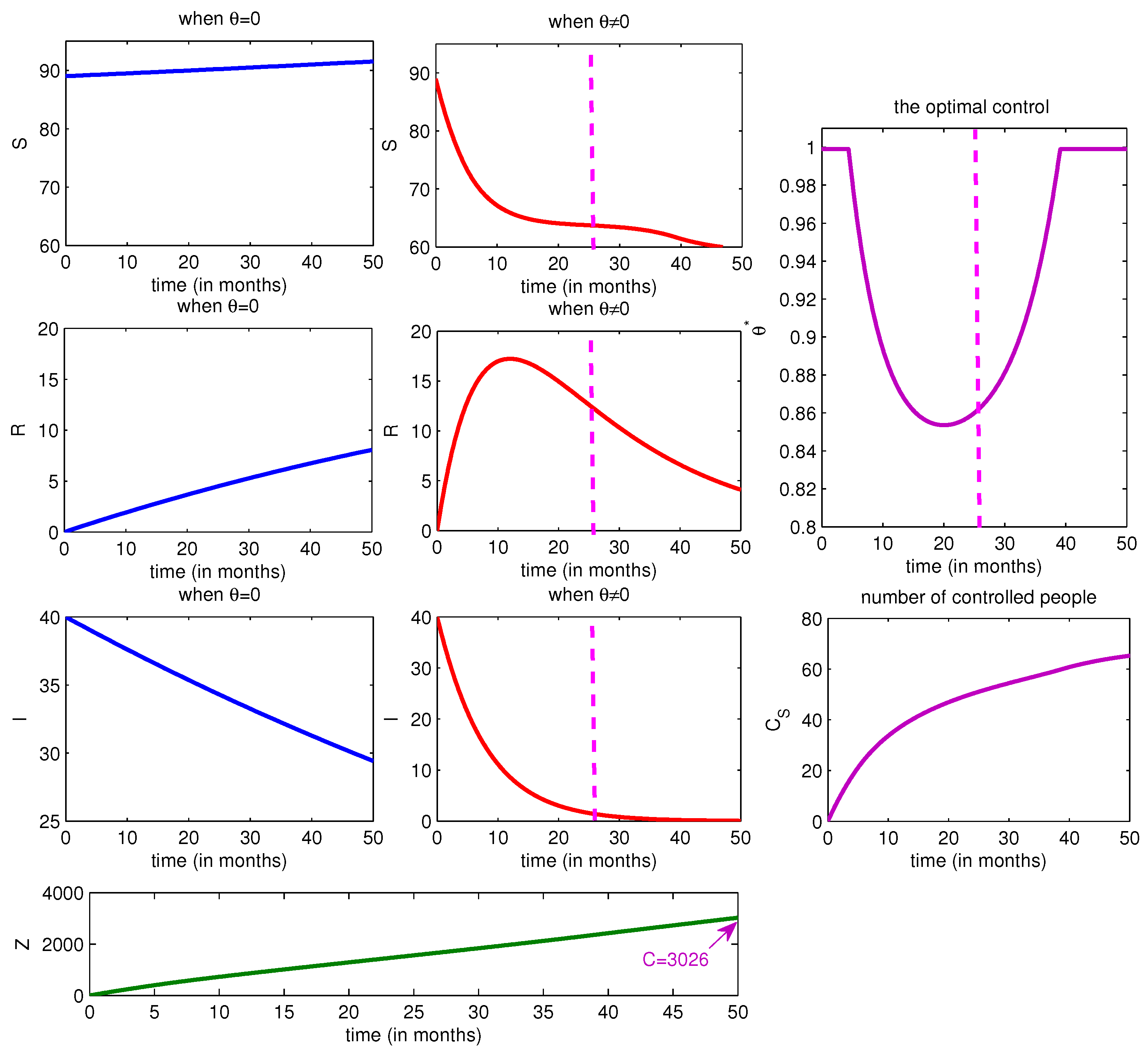
Figure 1 depicts the $S{C}_{S}IRZ$ dynamics in the absence and presence of the control and we can see that the number of susceptible people has increased linearly from its initial condition to a number higher than 92.5 individuals when we choose $\theta =0$, while the optimal state $S^{\ast }$ increases during the first months of the optimal control strategy and it decreases when we work with the characterization of Equation (11). Simultaneously, the number of removed people increases to only a value close to eight people while it reaches a value higher than this number with a maximal peak equaling to 17 when $\theta \ne 0$. As regards to the number of infected people, it decreases from its initial condition to a value close to an important value of 30 individuals because of the natural death and recovery only, while it decreases towards a value very close to zero after the introduction of the control $\theta$. We can see the relationship between the number of controlled people and the optimal values taken by $\theta$ so when this is increasing, the optimal state $C_S^{\ast }$ is also increasing. In fact, we can deduce that, with only small values of $\theta$, we reach our goal by minimizing I function, and maximizing R function while the total number of the susceptible who received the control along T and which is represented by the function Z has not exceeded the imposed constant C. The dashed lines introduced in this figure show the highest fixed point value of the sought final time, and we can understand that, at this point, we have already reached our goal which concerns the minimization of the number of infected people and maximization of the number of removed people. The next figure gives more information about the obtained value of $t_f^{\ast }$.

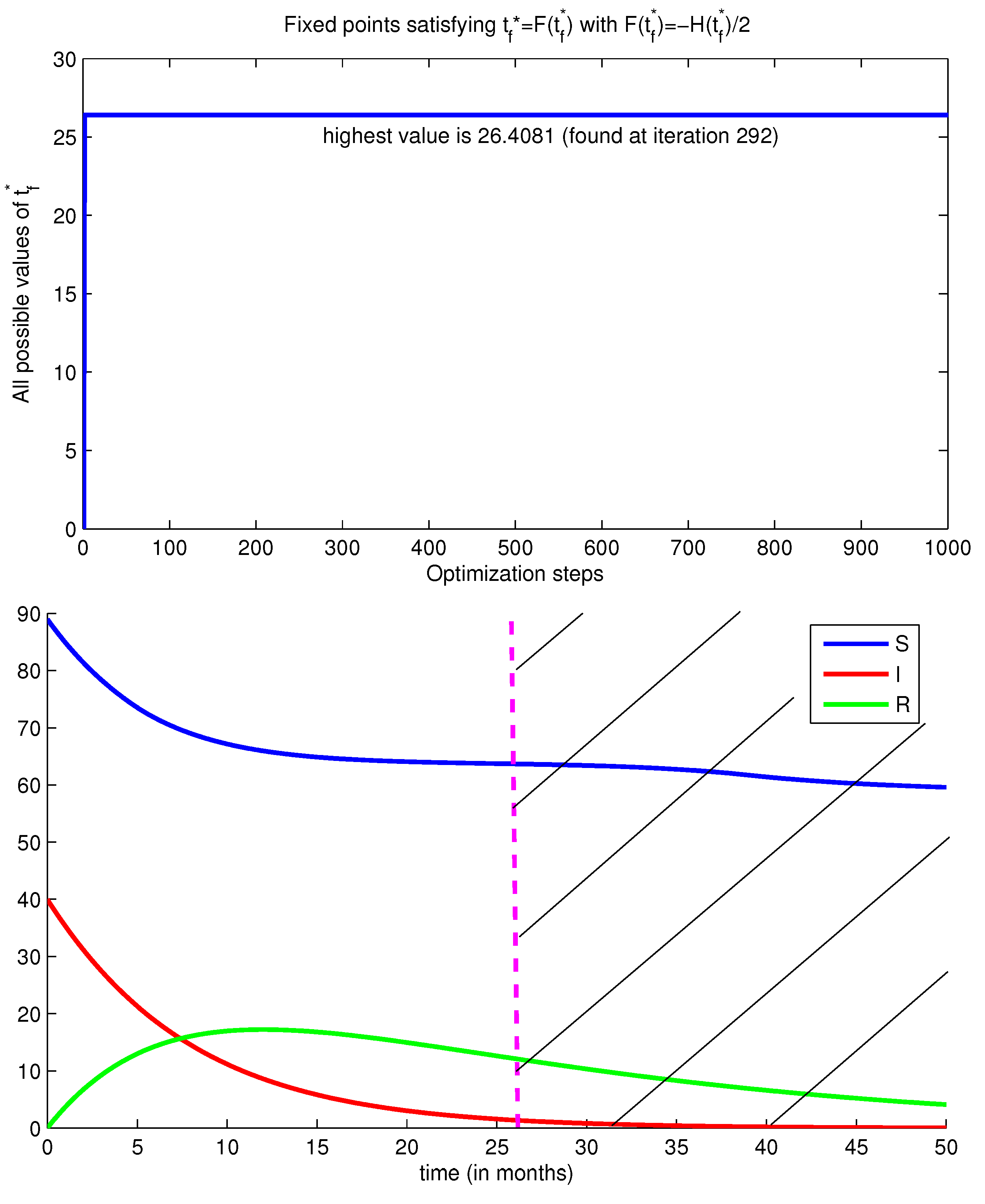
In Figure 2, we present dynamics of the functions S, I and R, and we can see the fixed points $t_f^{\ast }$ in the first plot above. The solution of the equation $F(t_f^{\ast })=t_f^{\ast }$ starts from an initial guess which equals zero, and increases to values that are very close or sometimes equal to 26 months (we note that, even if they appeared taking the value 26, this is not the case at all iterations but just because all values are very close to 26 with a small precision of about ${10}^{-4}$). As noted in this figure, for instance, the highest value of $t_f^{\ast }=26.4081$ found at iteration 292 among 1000. In the same figure, in the plot below, we observe that, at $t_f^{\ast }$ indicated by the dashed purple line, the number of infected people has already taken the direction towards zero values, while the number of removed people has already reached its positive peak and started to decrease because of the decrease of the optimal control function ${\theta }^{\ast }$, as shown in the previous figure. This means that there is no need in this case to extend the optimal control approach for other months since, at $t_f^{\ast }$, Equation (5) has been almost realized.

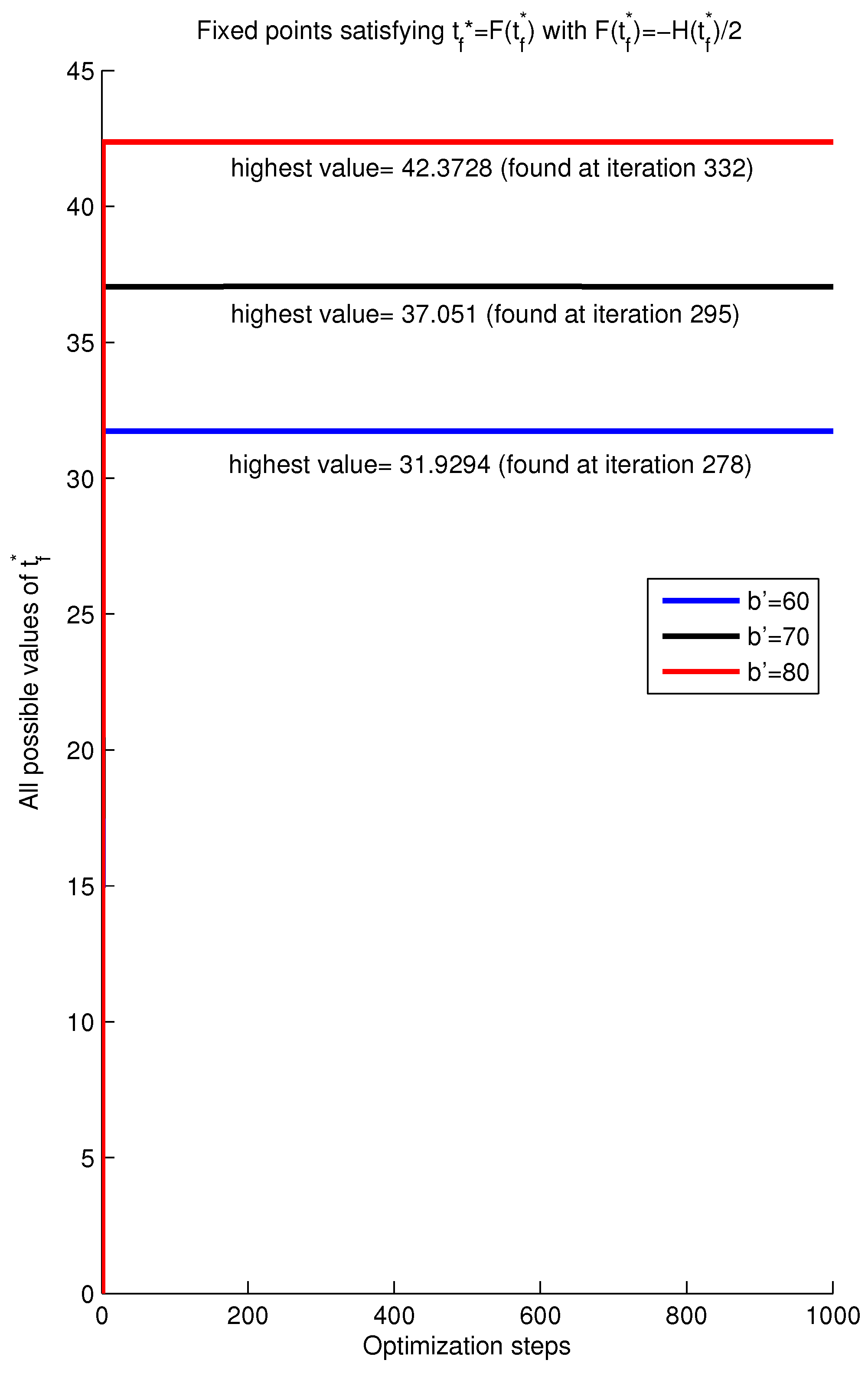
In Figure 3, the fixed points $t_f^{\ast }$ for different values of the control severity weight $b^{\prime }$ suggest that, as the value of $b^{\prime }$ increases, $t_f^{\ast }$ increases. In fact, the bigger is $b^{\prime }$, the lesser is the optimal control ${\theta }^{\ast }$, which is important, as we can deduce from the formulation in Equation (11), and this is reasonable since, when ${\theta }^{\ast }$ is small, we need more time to control the epidemic. The obtained results in this figure can be summarized as follows:

• When $b^{\prime }=60$: $I(t_f^{\ast })=6.734$ with $\theta (t_f^{\ast })=0.8658$ (iteration 278), which implies that $83.165\%$ of infected people have left the I compartment.
• When $b^{\prime }=70$: $I(t_f^{\ast })=6.0627$ with $\theta (t_f^{\ast })=0.8624$ (iteration 295), which implies that $84.8425\%$ of infected people have left the I compartment.
• When $b^{\prime }=80$: $I(t_f^{\ast })=4.7619$ with $\theta (t_f^{\ast })=0.8573$ (iteration 332), which implies that $88.09525\%$ of infected people have left the I compartment.

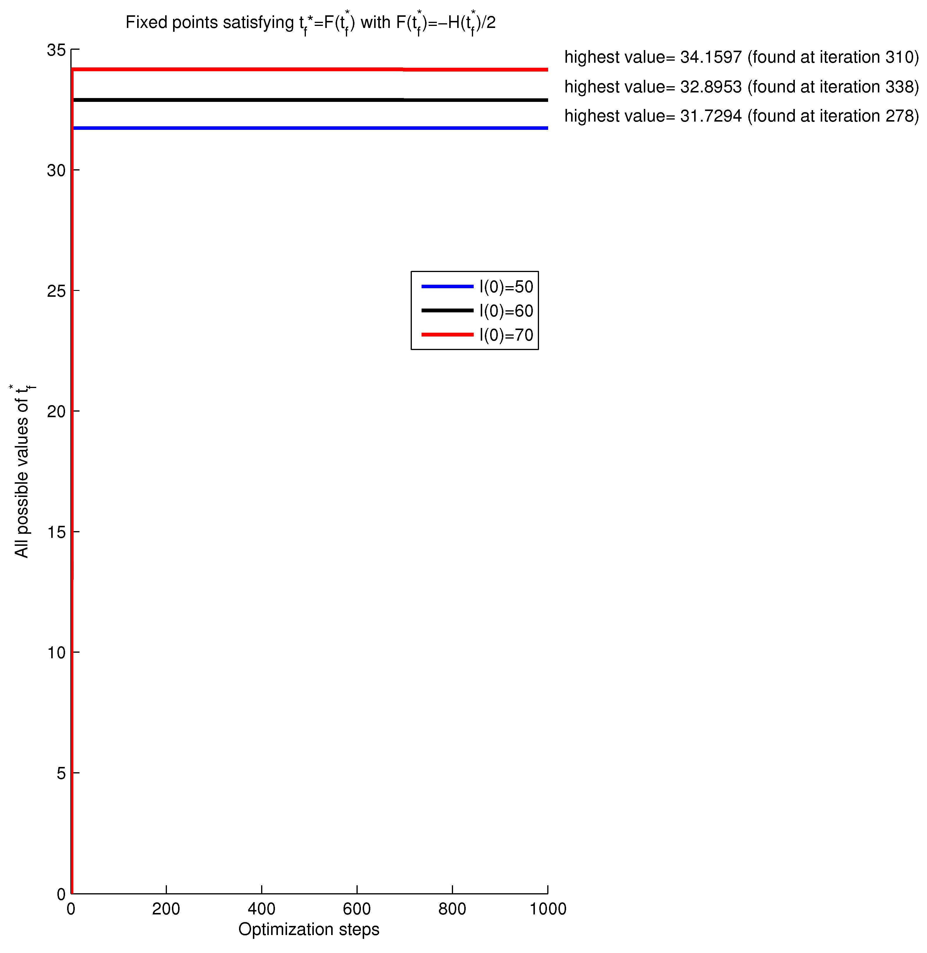
In Figure 4, we show the impact of the initial condition of I function, namely $I_0$, on fixed points $t_f^{\ast }$, and we can deduce from the obtained optimal horizons that, as $I_0$ increases, $t_f^{\ast }$ increases, and this is reasonable since, when the number of infected people is important, the anti-epidemic measures need longer time for controlling the situation. The obtained results in this figure can be summarized as follows:

• When $I(0)=50$: $I(t_f^{\ast })=8.4416$ with $\theta (t_f^{\ast })=0.8758$ (iteration 278), which implies that $83.1168\%$ of infected people have left the I compartment.
• When $I(0)=60$: $I(t_f^{\ast })=5.7018$ with $\theta (t_f^{\ast })=0.8662$ (iteration 338), which implies that $90.497\%$ of infected people have left the I compartment.
• When $I\left(0\right)=70$: $I\left(t_f^{\ast }\right)=8.1909$ with $\theta \left(t_f^{\ast }\right)=0.8802$ (iteration 310), which implies that $88.2987\%$ of infected people have left the I compartment.

5. Conclusions

In this paper, we have determined the optimal duration needed for controlling an epidemic based on a free horizon optimal control approach with an isoperimetric constraint and which has been applied to a four-compartmental epidemic model where it is supposed that the controlled population does not reach the removed class due to the temporary effect of the control. The isoperimetric restriction which has been proposed to define the number of susceptible people who receive the control along the anti-epidemic measures period, allowed us to find the optimal horizon of the optimal control strategy when there are limited resources devised to fight against a disease. In the numerical simulations, we used the fixed point method since the necessary condition on the free horizon led to a fixed point equation. Our results prove their usefulness, since, at the obtained optimal horizons for different values of parameters and initial conditions on infection, the infected population size has been reduced and this presents an advantage of the followed control approach to managers of the health resources even when these are limited.