Article

Differential Evolution Algorithm for Multilevel Assignment Problem: A Case Study in Chicken Transportation

by
Sasitorn Kaewman
1,*,
Tassin Srivarapongse
2,
Chalermchat Theeraviriya
3 and
Ganokgarn Jirasirilerd
4
1
Faculty of Informatics, Mahasarakham University, Maha Sarakham 44150, Thailand
2
Department of Economics, Rajamangala University of Technology Thanyaburi, Patumthani 12110, Thailand
3
Faculty of Engineering, Nakhon Phanom University, Nakhon Phanom 48000, Thailand
4
Faculty of Liberal Arts and Sciences, Sisaket Rajabhat University, Sisaket 33000, Thailand
*
Author to whom correspondence should be addressed.
Math. Comput. Appl. 2018, 23(4), 55; https://doi.org/10.3390/mca23040055
Submission received: 12 September 2018 / Revised: 30 September 2018 / Accepted: 30 September 2018 / Published: 2 October 2018
(This article belongs to the Special Issue Optimization in Control Applications)

Abstract

:
This study aims to solve the real-world multistage assignment problem. The proposed problem is composed of two stages of assignment: (1) different types of trucks are assigned to chicken farms to transport young chickens to egg farms, and (2) chicken farms are assigned to egg farms. Assigning different trucks to the egg farms and different egg farms to the chicken farms generates different costs and consumes different resources. The distance and the idle space in the truck have to be minimized, while constraints such as the minimum number of chickens needed for all egg farms and the longest time that chickens can be in the truck remain. This makes the problem a special case of the multistage assignment (S-MSA) problem. A mathematical model representing the problem was developed and solved to optimality using Lingo v.11 optimization software. Lingo v.11 can solve to optimality only small- and medium-sized test instances. To solve large-sized test instances, the differential evolution (DE) algorithm was designed. An excellent decoding method was developed to increase the search performance of DE. The proposed algorithm was tested with three randomly generated datasets (small, medium, and large test instances) and one real case study. Each dataset is composed of 12 problems, therefore we tested with 37 instances, including the case study. The results show that for small- and medium-sized test instances, DE has 0.03% and 0.05% higher cost than Lingo v.11. For large test instances, DE has 3.52% lower cost than Lingo v.11. Lingo v.11 uses an average computation time of 5.8, 103, and 4320 s for small, medium and large test instances, while DE uses 0.86, 1.68, and 8.79 s, which is, at most, 491 times less than Lingo v.11. Therefore, the proposed heuristics are an effective algorithm that can find a good solution while using less computation time.

1. Introduction

Thailand has long been known as a farming country due to the influence of Southeast Asian monsoons, which make the landscape, resources, environment, and climate conducive to agriculture. Most of the population works in agriculture or is involved in it in some manner. Although there have been efforts to develop Thailand into an industrialized country, it still largely depends on agriculture. The evolution and development of Thai agriculture has changed over time, reflecting the worldwide flow of changes. Hens are considered to be economic animals, as farmers can generate revenue from them throughout the year. In Thailand, there is a nationwide demand for eggs, which are popular among consumers. Breeding hens, therefore, are important to the economic balance and well-being of the Thai people. However, the problem that most farmers face is that they have high operating costs and generate little profit, thus they struggle to afford the costs incurred for labor, raw materials, transportation, etc.
In recent years, the logistics cost in Thailand is 14% of gross domestic product (GDP), which is valued at more than 1912.9 million baht. Many Thai businesses face the problem of high logistics cost, especially in agricultural businesses. In this study, we focus on reducing the cost of chicken transportation, which is one of the most important business groups of the Thai agricultural industry. Chicken transportation starts from delivering young chickens to egg farms in many different areas, which affects the resource usage of trucks (road conditions). It is not possible to travel on some Thai roads with some types of trucks, and even with some types of trucks the fuel consumption is different from the average speed limit. A suitable assignment approach needs to be decided on so that the total cost is minimized. Moreover, suitable trucks should be assigned to suitable chicken farms. Suitable farms and trucks means the truck does not have much idle space during delivery. Too much idle space means the use of bigger trucks, and bigger trucks always consume more fuel than smaller trucks because the weight of the truck affects the fuel consumption rate.
In transporting chickens from farmers to buyer farms, a number of factors must be taken into account—such as the mode of transportation, time to transport, temperature, etc.—as well as making sure that chickens from different farms are not mixed during transport. Therefore, it essential to find an appropriate vehicle that meets the needs of chicken farmers to avoid mixing chickens during transport to customers. This would help to minimize assignment or production costs and would be beneficial to the chicken farms, resulting in lower production costs and higher quality chickens for the egg farms. Thus, the overall condition of the chicken industry would be improved. Furthermore, chicken farms and egg farms can use the money saved to accomplish other farm activities, such as feeding, vaccinating, or researching—that is, to further develop their farms.
This study investigated a solution to the problem of chicken transport, which is a problem of multistate assignment. This was a case study regarding appropriate vehicle assignment for the transportation of chickens directly from chicken farms to egg farms by using the lowest cost of assignment. The differential evolution was developed to solve the problem because it is effective and uses short computation time. This paper has four contributions:
(1)
The special case of the multistage assignment problem is proposed. The attribute that makes it a special case is that the experience of the workers and the type of shipping instrument will be considered in the assignment of trucks to farms. These affect the time to ship chickens in trucks and will affect the total time that chickens can be in the trucks during transport.
(2)
The idle space in the truck is considered as the objective function and it is converted into lost opportunity due to higher fuel consumption of bigger trucks, therefore using unsuitable trucks will generate more cost.
(3)
The new decoding method of the DE algorithm is presented so that the proposed problem can be solved.
(4)
The mathematical model of the proposed problem is presented.
The paper is organized as follows. Section 2 presents the related research. Section 3 presents the problem statement and mathematical model. Section 4 shows the proposed heuristics (differential evolution algorithm). The computational result and a conclusion are presented in Section 5 and Section 6, respectively.

2. Literature Review

Assignment problem (AP): The AP evolved from the transportation problem, which is a form of proper task assignment to an employee or machine considering cost effectiveness or profit maximization in some cases. The assignment problem is a type of combinatorial problem. It has been addressed as a transportation problem, where transportation affects other jobs. The aim is to minimize the total cost of transportation. Therefore, this problem could be considered a task assignment problem [1]. The key condition of this problem is that the assignments must be on a one-on-one basis; that is, once a task has been assigned to an employee, it cannot be assigned to another employee as well.
Previously, task assignment problems were resolved by bipartite matching. This matching method was proposed by Frobenius and Konig [2,3]. Later, Dantzig [4] presented the assignment problem in the form of a linear programming problem and used the simplex method to solve it. However, there might be limitations on the size of the problem, the number of variables, and the number of constraint equations. This means that if the limitations were too great or the computer was not sufficiently capable, the simplex method would not work. Kuhn [5] subsequently presented a solution to assigning tasks through the Hungarian method, which is a quick way to solve problems compared to simplex.
Generalized assignment problem (GAP): GAP is more flexible than AP. Unlike AP, where assignments are made on a one-on-one basis, with GAP, one task can be assigned to multiple employees or to the same employee. However, it must not exceed the capacity of the employee. Thus, GAP is more comprehensive and more closely resembles the actual situation than AP. GAP was first proposed by Ross and Soland [6] and was found to be an NP-hard problem [7]. This is often corrected by the exact method with small problems. The problem of 200 tasks and 20 employees was considered to be the biggest problem that could be solved by the exact method [8]. Therefore, the heuristics method has been used to solve GAP.
The proposed problem is the multistage GAP. The GAP has no restrictions that the case study has, such as (1) the longest traveling time; (2) the effect of the shipping instrument and the experience of the workers, which affects the operating cost; (3) the idle space in the truck is considered as the objective function; (4) at least half of the demand of the egg farm has to be considered; and (5) the multistage GAP was never found in the literature.
We will move on to review the methodology to solve the special multistage assignment (S-MSA) problem. Many worldwide methods have been used to solve GAP. Both exact methods—such as branch and bound, branch and price, etc.—and heuristics methods have been used to solve the problem. Metaheuristics is one of the most commonly used methods to solve GAP. Metaheuristics is an approximation method where it is not guaranteed that the solution optioned from the method is the optimal solution. The advantage is that it uses much less computation time than the exact method, which makes it possible to solve real-world problems that cannot be solved by exact methods.
The well-known metaheuristics are the krill herd (KH) algorithm [9,10,11], the cuckoo algorithm [12,13], the monarch butterfly optimization (MBO) [14,15], the hybridizing harmony search [16], the Lévy-flight krill herd algorithm [17], the bat algorithm [18], elephant herding optimization (EHO) [19], and the earthworm optimization algorithm (EWA) [20].
Enhancing the quality of the heuristics method can be achieved in many ways, such as adjusting suitable parameters for the proposed method, increasing the search area by introducing ways to move from local optimal, and applying local search to increase the intensive search of the method [21,22,23,24,25]. The most recent successful method was proposed by Wang [26]. The method is called the krill herd (KH) algorithm. Many papers have proposed improving the solution quality of the KH, such as adding new attributes to the algorithm [22], using a hybrid KH with other methods [23,24,25,26], exchanging information between top krill during the motion calculation process [27], using the best parameters [28], and adding local searches to improve search ability [29]. Aside from being applicable to many types of problems, KH is valid for function optimization [30] as well. An excellent review of the KH method has been proposed by Wang et al. [31].
Metaheuristics has been applied to many combinatorial optimization and real-world problems, such as the parallel hurricane optimization algorithm [32], firefly-inspired krill herd (FKH) [33], the moth search (MS) algorithm [34], monarch butterfly optimization [35,36,37], across neighborhood search (ANS) [38], chaotic particle-swarm krill herd (CPKH) [39], chaotic cuckoo search (CCS) [40], self-adaptive probabilistic neural network [41], and the differential evolution (DE) algorithm [42].
Differential evolution is a frequently used heuristics method. It is a way to apply the principles of evolution, and the steps are as follows: (1) initial solution, (2) mutation, (3) recombination, and (4) selection. Differential evolution was first used by Storn and Price [43] and has since been used since to solve many problems, such as production scheduling [44] and manufacturing problems [45]. Liao et al. [46] proposed two hybrid DEs to obtain truck sequences for cross-docking operations. Later, Liao et al. [47] proposed six metaheuristic algorithms for sequencing inbound trucks for multi-door cross-docking operations under a fixed schedule of outbound truck departure. Hou [48] proposed discrete DE (DDE) by modifying a mutation operator for the vehicle routing problem (VRP) with simultaneous pickups and deliveries (VRPPD). Recently, Dechampai et al. [49] proposed DE to solve the capacitated VRP with the flexibility of mixing pickup and delivery services and maximum duration of a route in the poultry industry. Sethanan and Pitakaso [50] improved DE by adding two more steps, reincarnation and survival process, to improve its intensification search [51]. It has been proven that using different pairs of mutation and recombination processes gives different solution qualities, such as in Pitakaso and Sethanan [50] and Boon et al. [52]. Sethanan and Pitakaso [50,51] suggested that improving the DE algorithm, such as by adding more steps to the original DE, inserting local search, and adding more attributes, can improve the solution quality, but the design of the decoding method must make sure that the most important rules in solution quality are obtained. In this paper, the excellent design of a decoding method from real numbers obtained from the DE mechanism to find the solution of the proposed problem is reported. The decoding method not only makes it possible to obtain the solution, but also local search has been added to the decoding method routine. Therefore, excellent results can be gained from the proposed method.

3. Problem Statement and Mathematical Modeling

This section explains the problem statement and the mathematical model to represent the problem so that the reader has more understanding of the proposed problem.

3.1. Problem Statement
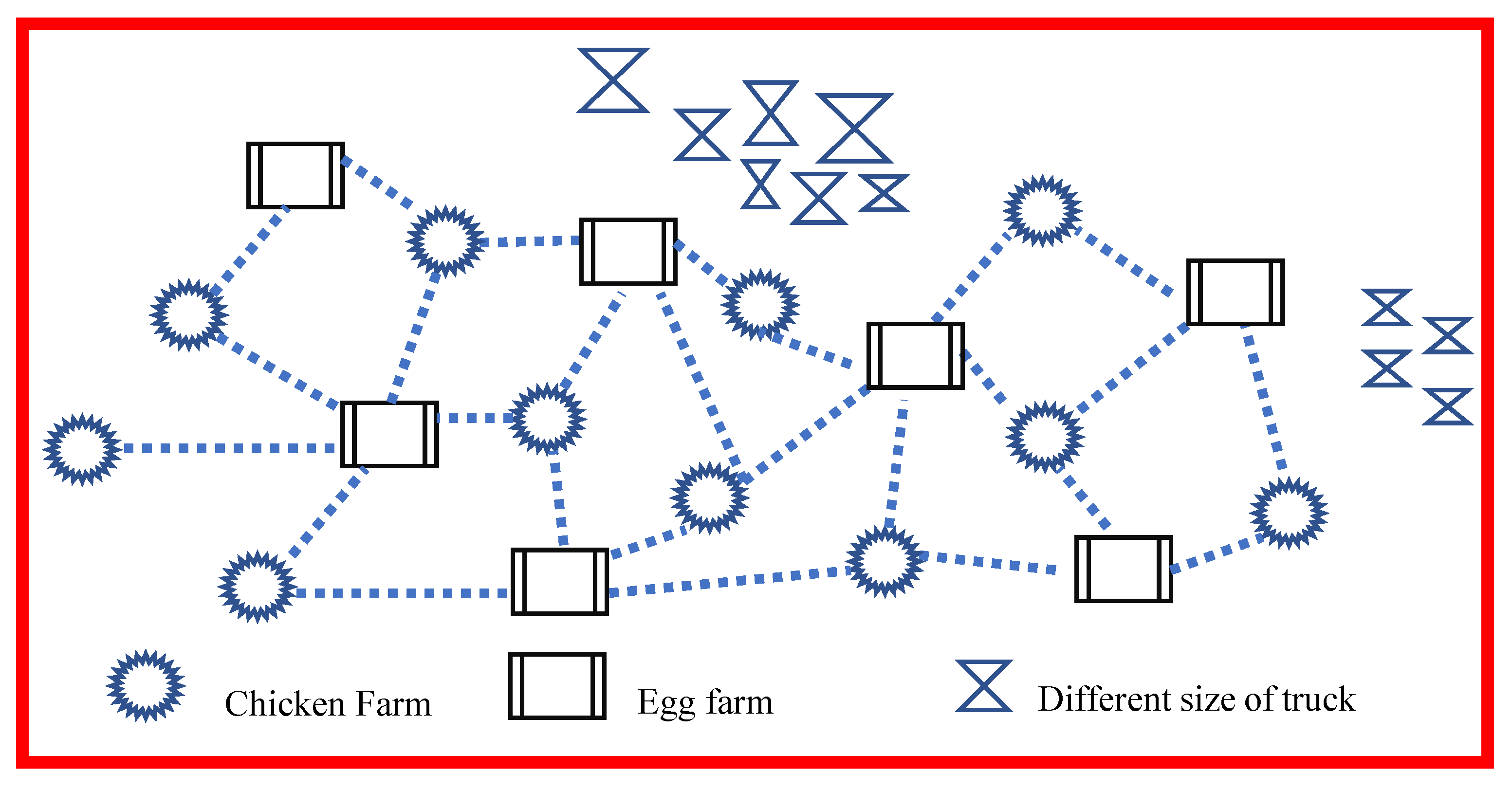
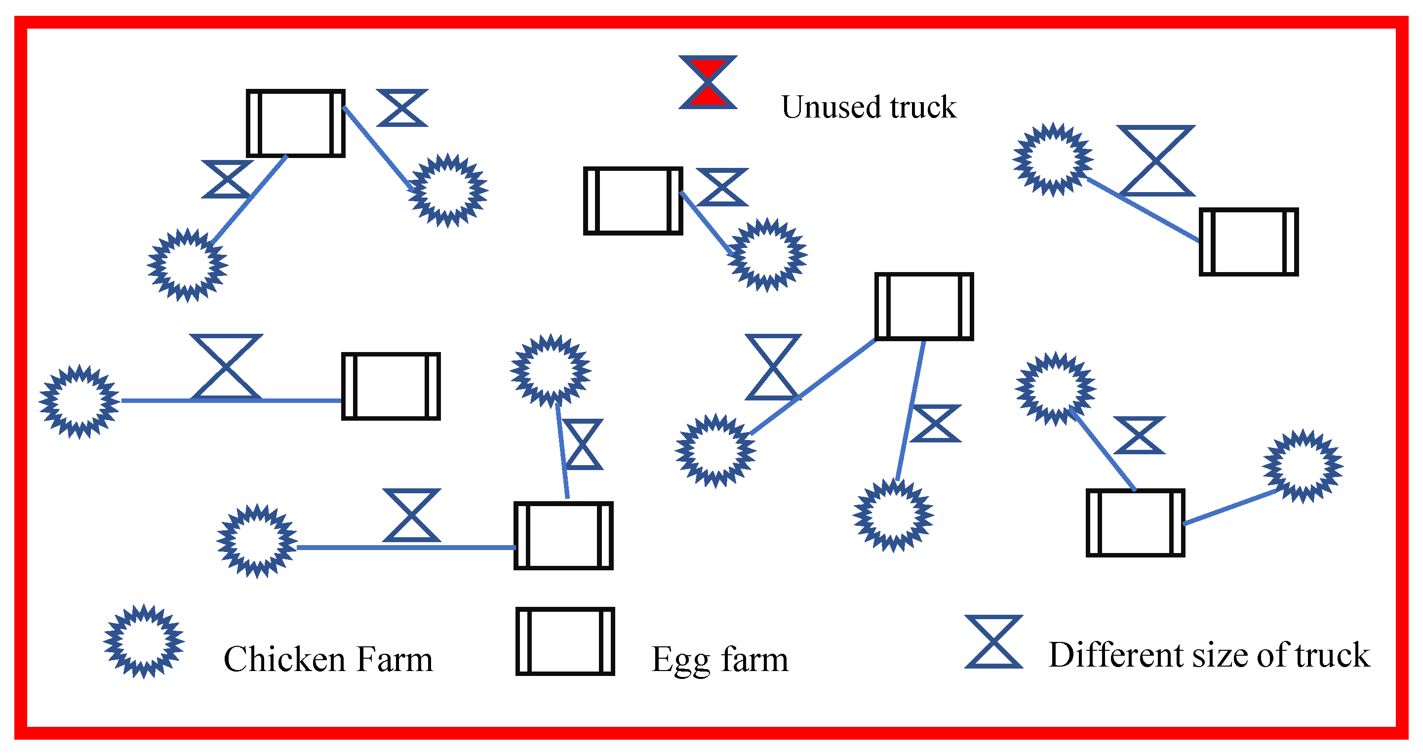
Figure 1 and Figure 2 represent the unsolved problem and the solved problem, respectively. Chicken farms have different amounts of young chickens. The chicken farms transport the chickens to egg farms, which grow the chickens and collect the eggs to sell to end customers. The egg farms have different capacities and demands for young chickens from chicken farms. The transportation of chickens needs to use trucks. The chicken farms have workers and loading/unloading instruments such as forklifts, carts, etc. This can make for different delivery times for the chicken farm in different types of trucks. When the truck arrives at the egg farm, the egg farm also has instruments for unloading chickens from the truck, which causes different shipping times. The objective function is not only to minimize the total distance of assignment under many constraints, which will be explained later, but also to minimize the idle space of the truck when transporting chickens. The idle space is assumed to be a lost opportunity to use the suitable truck for the suitable route. Moreover, it is possible that some trucks are not used. Therefore, the problem comprises the following components:
(1)
Assign the right truck to the right egg farm so that free space is minimized. Different farms have different levels of experience with different trucks, which can affect the loading of chickens onto the truck, which can affect the total time that the chickens are in transport.
(2)
Assign the right egg farm to the right chicken farm to minimize so travel distance. The workers at the chicken farm and the egg farm need to be coordinated so that shipping chickens out on the trucks uses as little time as possible, therefore the quality of the chickens remains unchanged.
The problem is a special case of the multistage assignment problem (S-MAP). The objective function is to minimize total distance and minimize free space in the truck. This objective needs to be optimized while keeping the following limitations or constraints:
(1)
Transportation of chickens from chicken farms to egg farms is done only by direct transport. There is no chicken picking from other farms and no eggs are sent to other farms. This is because egg farms need to control the quality and breed of the chickens and prevent communicable diseases.
(2)
A chicken farm can send chickens to an egg farm more than once.
(3)
A chicken farm can sell all of its chickens.
(4)
Egg farms may receive chickens from more than one farm, but they may not exceed the capacity of such farms.
(5)
Egg farms will receive chickens for at least 50% of the demand. However, some egg farms may not be able to do this. Transportation time should not exceed 8 h, which includes the time spent loading the chickens onto the vehicle, transfer, and removal.
(6)
The vehicles used for transport are sufficient for the needs.
(7)
Chicken farms may use more than one type of vehicle and each type can be used for more than one round.
There are 40 chicken farms in the case study, and the capacity of a chicken farm is from 5000 to 20,000 chickens per planning period. There are four types of truck available, which have a capacity of 2000 to 12,000 chickens per round of travel. There are 60 egg farms in the system, for which chicken farms need to deliver at least 50% of the demand.

3.2. Mathematical Modelling

The S_MAP can be modeled as follows:
Indices
i = 1, 2, 3, 4 (4 truck types)
j = 1, 2, 3, …, J (J number of chicken farms; 40 farms)
k = 1, 2, 3, 4 (4 rounds of transportation)
l = 1, 2, 3, …, L (L number of egg farms; 60 farms)
Decision Variables
x i j k l Decision variable
x i j k l = 1 Truck (i) is assigned to transport chickens from chicken farm (j) on the round of transporting (k) to egg farm (l)
x i j k l =   0 Truck (i) is assigned to transport chickens from chicken farm (j) on the round of transporting (k) to egg farm (l)
q i j k l Number of chickens transported by truck (i) from chicken farm (j) on round (k) to egg farm (l)
Parameters
c i j l Cost of truck type assignment (i) to transport chickens from farm (j) to egg farm (l)
t i Capacity of truck (i) to transport chickens (unit: chicken)
o c i j l Cost of lost opportunity due to truck not completely loaded (i) from chicken farm (j) to egg farm (l) (unit: baht per chicken)
d l Demand for chickens by egg farm (l)
s j Capacity of chicken breeding of farm (j)
t u p i j Time spent loading chickens onto truck (i) at chicken farm (j)
z u p i j Performance of employees at chicken farm (j) to carry chickens into truck (i)
t d n i l Time spent removing chickens from truck (i) at egg farm (l)
z d n i l Performance of employees at egg farm (l) to remove chickens from truck (i)
t t r i j k l Time spent traveling from the truck station to chicken farm (j) then to egg farm (l), and then from egg farm (l) back to the truck station
t d j l Time spent for truck (i) to go from the station to chicken farm (j) to convey chickens on round (k) to egg farm (l)
t i m e j k l Time spent for an assignment of each round, not to exceed 8 h, consisting of the time to load chickens at chicken farm (i) ( t u p i j k l ) , time to transport from farm (i) to egg farm (l) ( t t r i j k l ) , and time to remove chickens from the truck at egg farm (l) ( t d n i j k l ) , or the overall time to use the truck
t t r u c k i Usage time of truck type
Remark 1.The time for t t r i j k l and t d i j k l does not include the usage time to load and remove chickens from the truck.
Objective Function
m i n i I j J k K l L ( c i j l × x i j k l ) Part 1 + i I j J k K l L [ ( ( x i j k l × t i ) q i j k l ) Part 2 × o c i j l ]
  x i j k l { 0 , 1 }         f o r       i j k l  
  q i j k l { 0 , 1 }             f o r       i j k l  
  l L x i j k l 1             f o r       i j k  
i I j J k K q i j k l d l           f o r       l  
i I j J k K q i j k l 0.5 × d l           f o r       l  
i I k K l L q i j k l = s j             f o r       j  
  q i j k l M × x i j k l             f o r       i j k l  
  q i j k l t i           f o r       i j k l  
  t u p i j = z u p i j × q i j k l             f o r       i j k l  
  t d n i l = z d n i l × q i j k l         f o r       i j k l  
  t t r i j k l = t d j l × x i j k l           f o r       i j k l  
  t i m e i j k l = t u p i j k l + t d n i j k l + t t r i j k l             f o r       i j k l  
  t i m e i j k l 8             f o r       i j k l  
j J k K l L t i m e i j k l t t r u c k ( i )         f o r       i  
  x i j k l x i j ( k + 1 ) l         f o r       i j k l  
This mathematical model was created to solve multistage assignment problems. The objective function aims to investigate how to assign the task in order to gain the lowest cost of the assignment, for which distance is the key factor (part1 of Equation (1)). The cost of opportunity loss is due to the truck not being completely loaded. This means that there is free space on the truck for each round of transporting (part2 of Equation (1)).
The relevant limitations begin from the decision variables ( x i j k l ) , which are the counting numbers and equal to 0 or 1 only (Equation (2)). The number of chickens prepared for transport ( q i j k l ) must be equal in the positive integer only (Equation (3)). Egg farm (i) can receive chickens from farm (j) by using truck (i) for transportation round (k) only one time (Equation (4)). Epidemics may be prevented because chickens are transported from different places, and an egg farm (l) may not receive as many chickens as it needs (Equation (5)). Each egg farm (i) will receive at least 50% of the chickens it needs (Equation (6)). Each chicken farm (j) will be able to deliver all chickens to the egg farm until there are no more chickens at the farm (Equation (7)). If there is no assignment ( x i j k l = 0 ) , the number to transport is equivalent to 0 ( q i j k l = 0 ) as well (Equation (8)).
The quantity to be transported (q) in each round shall not exceed the capacity of the truck (Equation (9)). The time spent loading chickens onto the truck is represented by Equation (10). The quantity of chickens to be transported (q), the performance of the workers in loading chickens (zup), and the time taken to remove chickens from the truck are represented by Equation (11). The quantity of chickens to be transported (q), the performance of the workers in removing chickens from the truck (zdn), and the time spent on transportation ( t t r i j k l ) from the station to the chicken farm, and then from the chicken farm to the egg farm, and finally getting back to the station, which does not include time for loading and removing chickens, depends on distance and driving speed (Equation (12)). Equation (13) is the overall time for an assignment. The time spent loading chickens (tup), time spent traveling (ttrans), and time spent removing chickens from the truck (tdn) must not exceed 8 h (Equation (14)). The usage time of each type of truck may not exceed the working hours that have been set (Equation (15)). Equation (16) fixes a round of assignments starting at the first round.

4. Proposed Algorithm

The proposed method that is used to solve the S-MSA is the differential evolution (DE) algorithm. DE comprises four steps: (1) initialize the target vectors, (2) perform the mutation process, (3) perform the recombination process, and (4) perform the selection process. The proposed method can be explained as follows.

4.1. Initial Vector (Initial Population)

This step requires defining the number of the population and the random number of the population. The population must be at least four, because the DE process uses three vectors to determine the direction of the searching. If the population is small, it will not spread to find the answer. When the initial population is determined, it will be entered into the encoding process as the next DE method. The end product of this step is the first target vector.
The initialization needs to generate the vector representing the problem solution. We call it encoding. The encoding is the coding for three factors, such as the type of truck, chicken farm, and egg farm. In this case study, there are five vectors and each vector has four positions. This process starts by specifying a random number for each position in each vector, for which the random numbers are equivalent between 0 and 1, as shown in Table 1, Table 2 and Table 3 respectively.
From the random number of the position in each initial vector, the initial vectors of truck type, chicken farm, and egg farm are sorted by random numbers. The lowest of the random numbers is set to be in the first position. The higher random numbers will be set in the last row of each column, as shown in Table 4, Table 5 and Table 6.
For this study, first, vectors of truck type, chicken farm, and egg farm were assigned. The lowest random number, or position no. 1, was selected as the first order, as shown in Table 7.
The vectors shown in Table 1, Table 2, Table 3 and Table 4 need to be decoded to get the proposed problem’s solution. This step is called decoding. Decoding is the sequential ordering in the assignment table, as shown in Table 8, to encode. For the operation of decoding, all constraints must be accomplished at the same time. For example, each type of truck cannot be overloaded and must not exceed the specified working hours. The working hours start from the time spent loading chickens at chicken farms. Travel time includes the time to travel from the station to the chicken farm and from the chicken farm to the egg farm, including the time to get back to the station and the time to remove chickens from the truck at the egg farm. The chicken farm can deliver all of the chickens without the rest of the chickens at the farm. The first assignment must be completed before another assignment can be given to the chicken farm. The egg farm will receive at least 50% of the demand in the beginning, after which more chickens will be added. The chicken farm in the first sequence usually receives the amount of chickens it demands. However, the farm in the latter sequence may not get the number of chickens it wants. All factors involved must be considered simultaneously. An important factor in task assignment is the quantity assigned each time, which will be affected by the type of truck and the number of rounds, which includes transportation costs. The amount of chickens to be transported ( A s s i g n Q ) is determined by the number of chickens from one farm, including the demand from the egg farm to assign up to 50% of its demand before providing the rest. The transported chickens are counted from the quantity of chickens at the farm and the demands of the egg farm. If any quantity is less, it will be transported using such a quantity. The assignment is shown in Equation (17)
  A s s i g n Q = { Q d A   i f Q d Q s Q s   o t h e r w i s e
A s s i g n Q means quantity to be transported, Q d A means the initial chicken demands of the egg farm equivalent to 50% of the entire demand, and Q s means productivity of the chicken farm.
Another factor is the quantity to carry, which has a great influence on the type of truck selected. Choosing the proper vehicle will save transportation costs. If a truck is chosen that has less capacity than the amount it is required to carry, it will require several trips to complete the transport. This results in fuel consumption and increases transportation cost. If a truck is chosen that is larger than the amount to transport, there is free space, which raises the cost. Therefore, selecting the truck type should be based on a capacity that is larger than—but similar to—the quantity to be delivered, to avoid several rounds of transportation, which could cost more than a single trip with a large truck, as shown in Equation (18)
m i n   T r u c k Q k A s s i g n Q  
T r u c k Q k means the capacity of truck type k; k = 1, 2, 3, and 4.
The assignment of chicken farms will be carried out in the order shown in Table 10, starting from the initial order farm since the first farm has been completely assigned. Then, another farm can be assigned when the all farms have been assigned and no chickens remain. The assignment for the egg farms is different, as they require at least 50% of their demands. After that, additional chickens will be provided. The chicken farm in the first sequence usually receives the amount of chickens it demands. However, the farm in the latter sequence may not get the chickens it wants. Once the assigned quantity has been determined, the type of vehicle will be assigned. Also, the second round of transport will take place when the same vehicle is assigned from the same chicken farm to the same egg farm until the requirement is met. With the initial decoding for an assignment to provide 50% of chickens to egg farms as the limitation, the first assignment is shown in Table 8, in which chicken farm no. 2 has been assigned as the first and has an order of 5000 chickens, while the first egg farm needs 10,000 chickens. Therefore, this egg farm will receive at least 50% of its demand (5000 chickens) from chicken farm no. 2. To avoid several rounds of transportation, trucks that have more capacity than the assigned quantity are used.
However, choosing a more capable truck will result in costs of lost opportunity. In order to avoid this cost, trucks should be selected with a capacity closest to the quantity to be commissioned. In the case of 5000 chickens, this will be assigned to a truck that has capacity for 8000 chickens, which also results in 3000 empty spaces and lost opportunity cost.

4.2. Perform Mutation Process

Mutation is a method of modifying the values in the vector position, which is a step to extend the scope for finding the answers. It starts from three random vectors from the initial population in the same group (truck type, chicken farm, and egg farm), combining the first vector with the difference from the other two to form a new vector. This principle is unique to differential evolution and can be expressed as
  v i , j , G + 1 = x r 1 , j , G + F ( x r 2 , j , G x r 3 , j , G )  
  • x r 1 , j , G = target vector ( r 1 ) of chicken farm group (j) acquired from random G population, for which there are three vectors, and the next vectors are x r 2 , j , G and x r 3 , j , G.
  • v i , j , G + 1 = mutant vector, or the vector from the steps of modifying the values of the vector in population position (i) of vector group (j) for the new population (G + 1).
  • F = mutant factor; F is equal to 0.8 (Qin et al., 2009), acquired from the experiment to find the optimal value.
  • i = 1, 2, 3, …, N (N means the number of population).
  • j = 1, 2, 3 means the vector from type of truck, chicken farm, and egg farm, respectively.
The target vectors of truck type, chicken farm, and egg farm, as shown in Table 1, Table 2 and Table 3 respectively, are taken into the modification of the vector position to obtain the mutant vector of the truck type (Table 9), of the chicken farm (Table 10), and of the egg farm (Table 11). Evaluating the mutant vector, F = 0.8 [53], this is a good starting point to randomly select three vectors from X i , G and then substitute them into Equation (19), which produces 0.853 + 0.8 (0.757–0.335), which is equal to 1.191. Then, it leads to the recombination of the vectors.

4.3. Perform the Recombination Process

The recombination process uses the mutant vector ( v i , j , G ) and the target vector ( x i , j , G ) to select once again to be a trial vector ( u i , j , G ) by choosing only one vector. The process must not choose the same vector. The method can be expressed as
u i , j , G = { v i , j , G       w h e n       C R r a n d x i , j , G       w h e n       C R > r a n d  
The recombination method aims to use the target vector from the first step to find the difference of vectors in the mutant vector of position but still allow the target vector to return to the process by setting the crossover rate (CR) to 0.2. If the random number for each vector is greater than or equal to a CR of 0.2, the mutant vector will be selected. If the random number is less than the CR, the target vector will be selected, as shown in Table 12.
Applying the random number obtained from Table 12 to the mutant vector demonstrates that most of the vectors taken into consideration in the vector selection procedure were the ones that already passed the mutant vector process. The selected vector of the truck type is shown in Table 13, that of the chicken farm is shown in Table 14, and that of the egg farm is shown in Table 15. Then, the vector selection procedure continues.

4.4. Perform the Selection Process

The selection process is the vector selection step in DE that compares the cost of assignment (fitness function) with the cost of the target and trial vectors from the mutation process.
x i , j , G + 1 = { u i , j , G + 1 i f f ( u i , j , G + 1 ) f ( x i , j , G ) x i , j , G o t h e r w i s e
If the cost of the assignment from the trial vector is less than or equal to the cost of the assignment from the target vector, then the trial vector will be selected and collected for the next population. On the other hand, if the cost of the assignment given by the trial vector is greater than the target vector, then the target vector will be collected from this population to be the vector for further population. Repeat steps 2–6 until the best answer is acquired.
From the explanation in Section 4.1, Section 4.2, Section 4.3 and Section 4.4, the proposed heuristics procedure is shown in Algorithm 1.
Algorithm 1. Pseudocode of the proposed heuristics.
Set NP, CR, F, NP (size of vector)
Generate initial solution
Begin
For G = 1 to Gmax, where G = iterations and Gmax = maximum iterations
For N = 1 to NP
Generate random target vector X r 1 , j , G and RV and update BV
Produce mutant vector N (mutation process) (Equation (19))
v i , j , G + 1 = x r 1 , j , G + F ( x r 2 , j , G x r 3 , j , G )
Produce trial vector N (recombination process)
     • Using Equation (20):
u i , j , G = { v i , j , G       w h e n       C R r a n d x i , j , G       w h e n       C R > r a n d
   Produce new target vector (selection\process)
X i , j , G + 1 = { U i , j , G i f   f ( U i , j , G ) f ( X i , j , G ) X i , j , G otherwise
End

5. Computational Framework and Result

The proposed heuristics were executed and compared with the solution generated by Lingo v.11. We reprogrammed the proposed heuristics in C++ and simulated it on a computer with Intel (R) Core i7-3520M CPU @ 2.90 GHz Ram 8.00 GB. We tested our algorithms with three groups of test instances, small, medium, and large. The simulation was executed five times until the best solution was selected, as shown in the table. Details of the test instances are shown in Table 16.
From Table 16, we test our 37 tested instances, composed of 12 small, medium, and large instances and 1 case study. For small and medium test instances, the proposed method was compared with the exact method. The exact method used here is Lingo v.11. For the large instances and the case study, the proposed method was compared with the lower bound generated by Lingo v.11 within 72 h.
The first experiment was executed with the small and medium test instances. The stopping criterion for Lingo v.11 was when it found the optimal solution. The best solution and computation time were collected. The stopping criterion for DE was when it found the optimal solution (the same as Lingo v.11) or when it reached 500 iterations. The results are shown in Table 17 and Table 18 for small and medium randomly generated datasets, respectively. The simulation was executed in 12 test instances, each of which had a size of 5 × 5 (number of egg farms × number of chicken farms). The best solutions out of five runs are shown in Table 17 and Table 18.
Table 17 shows a small group of problem instances. In one out of five instances, the proposed heuristic could not find the optimal solution. The average gap (%diff.) of DE from the solution generated by Lingo v.11 was 0.03% and it used 10.57 times (9.09/0.86) less computation time. The simulation was executed for 12 test instances, each with a size of 10 × 10 (number of egg farms × number of chicken farms). The best solutions out of five runs are shown in Table 18.
Table 18 shows a medium-sized test, for which the sample size is 10 × 10. Lingo v.11 took 100.83 s on average to find a 0.05% better solution than DE, but DE used only 1.68 s computation time on average to find that solution.
The next experiment was executed with a large size of test instances. The stopping criterion of Lingo v.11 was 72 h or 4320 min. The best solution found within that time was collected to compare with the result generated by DE. The stopping criterion of DE was set at 1000 iterations. The solution is shown in Table 19. This group includes the case study (40 × 60).
Table 19 shows a large-scale problem test, for which the sample size was 20 × 20. The result generated by Lingo v.11 within 72 h had an average cost of 51,576.46 baht, while the result generated by DE was 49,622.46 baht, or 4.52% less, using 491 times less computation time. The comparison of Lingo v.11 and DE shown in Table 17, Table 18 and Table 19 was statistically tested using Wilcoxon signed-rank test with 95% confidence interval. The statistical test results are shown in Table 20.
From Table 20, we can see that in the small and medium groups, the performance of DE and Lingo v11 was not significant different, and for the large size, DE had significantly lower cost than Lingo v.11.

6. Conclusions and Suggestions

The purpose of resolving the multistage assignment problem is to minimize the cost of assignment. The case study in this research consisted of the main cost of transportation, which relies on the distance to transport as well as the cost of opportunity loss related to truck incapacity.
The resolution started from the development of a mathematical model that consisted of the cost of chicken transportation and opportunity loss. The model had to comply with the conditions as well. Then, the mathematical model was applied to find the best answer using Lingo v.11. Unfortunately, when the problem size is large, Lingo v.11 is not able to solve the problem into optimality, therefore the metaheuristics have to be further developed to get the solution for the case study and the large problem size.
Later, DE was developed to solve the multistage assignment problem, and the results of the efficiency of DE vs. Lingo v.11 were compared. In the case that Lingo v.11 can find the optimal solution, we compared the proposed heuristic (DE) with the optimal solution. The time Lingo v.11 used to find the optimal solution was recorded for all test instances. In this case, DE will use number of iterations (set to 500 from the preliminary test). The computation results show that in small- and medium-sized test instances, DE uses much less computation time than Lingo v.11 while obtaining less than a 1% cost difference (0.03% and 0.05%, respectively) from the optimal solution. In the large-sized problem instances, DE found a 3.52% better solution while using 491 times less computation time than Lingo v.11. Thus, we can see that the performance of DE is better when the problem size is larger. DE obtains better solutions than Lingo v.11 when it uses much more computation time. DE is suitable to solve big problems that an exact method like Lingo v.11 cannot solve.
From the computation results shown in Table 18, Table 19 and Table 20 we can see that when the problem size is small, Lingo v.11 can always find the optimal solution and DE sometimes has worse solution quality than Lingo v.11. This is the weak point of the proposed heuristics: in small- and medium-sized test instances, it cannot find the optimal solution even when we increase the iterations to 1000 or 1500. This means that, in small-sized test instances, DE converts fast and sticks on the local optimal. When there is a large size of test instances, DE can find a better solution than Lingo v.11, because when the problem size is large, it is hard for the exact method to solve to optimality, and when the computation time is set at 72 h, Lingo v.11 is not yet finished with the search while DE, the metaheuristic, can finish the search activity.
Future research should study more complicated assignment problems as well as the current problems or other metaheuristic methods to enhance solutions through hybrid methodologies. Algorithm designers need to add a search mechanism that allows the proposed solution to escape from the local optimal to the general mechanism of DE so that the ability to escape from the local optimal will be increased.

Author Contributions

S.S. designed the algorithm; T.S. and C.T. gathered data and programed the algorithm; G.J. made the summary and conclusion.

Funding

We would like to express our thanks to Mahasarakham University, Rajamangala University of Technology Thanyaburi, Ubon Ratchathani University, Nakhon Phanom University, and Sisaket Rajabhat University for funding this project.

Conflicts of Interest

The authors declare no conflict of interest.

References

  1. Monge, G. Sur le CalculIntégraldes Équations Aux Differences Partielles. Available online: http://verbit.ru/MATH/TALKS/India/History-MA.pdf (accessed on 10 May 2016).
  2. Frobenius, F.G. Ferdinand Georg Frobenius; Gesammelte Abhandlungen, Band III; Serre, J.-P., Ed.; Springer: Berlin, Germany, 1968. [Google Scholar]
  3. Konig, D. Vonalrendszerek és determinánsok. Mathenatikaies Termeszettudomanyi Ertesito 1915, 33, 221–229. [Google Scholar]
  4. Dantzig, G.B. Application of the simplex method to a transportation problem. In Activity Analysis of Production and Allocation, Proceedings of Linear Programming, Chicago, Illinois, 1949; Wiley: New York, NY, USA, 1951; pp. 359–373. [Google Scholar]
  5. Kuhn, H.W. The Hungarian method for the assignment problem. Nav. Res. Logist. Q. 1956, 2, 83–97. [Google Scholar] [CrossRef]
  6. Ross, G.T.; Soland, R.M. A branch and bound algorithm for the generalized Assignment problem. Math. Program. 1975, 8, 91–103. [Google Scholar] [CrossRef]
  7. Fisher, M.L.; Jaikumar, R. A generalized assignment heuristic for vehicle routing. Networks 1981, 11, 109–124. [Google Scholar] [CrossRef]
  8. Liu, L.; Mu, H.; Song, Y.; Luo, H.; Li, X.; Wu, F. The equilibrium generalized Assignment problem and genetic algorithm. Appl. Math. Comput. 2012, 218, 6526–6535. [Google Scholar] [CrossRef]
  9. Wang, G.; Tan, Y. Improving Metaheuristic Algorithms with Information Feedback Models. IEEE Trans. Cybern. 2017, 99, 1–14. [Google Scholar] [CrossRef] [PubMed]
  10. Wang, G.; Guo, L.; Gandomi, A.H.; Hao, G.; Wang, H. Chaotic Krill Herd algorithm. Inf. Sci. 2014, 274, 17–34. [Google Scholar] [CrossRef]
  11. Wang, G.; Gandomi, A.H.; Alavi, A.H. An effective krill herd algorithm with migration operator in biogeography-based optimization. Appl. Math. Model. 2014, 38, 2454–2462. [Google Scholar] [CrossRef]
  12. Cui, Z.; Sun, B.; Wang, G.; Xue, Y.; Chen, J. A novel oriented cuckoo search algorithm to improve DV-Hop performance for cyber-physical systems. J. Parallel Distrib. Comput. 2016, 103. [Google Scholar] [CrossRef]
  13. Wang, G.; Alavi, A.H.; Zhao, X.; Hai, C.C. Hybridizing harmony search algorithm with cuckoo search for global numerical optimization. Soft Comput. 2016, 20, 273–285. [Google Scholar] [CrossRef]
  14. Feng, Y.; Wang, G. Binary Moth Search Algorithm for Discounted {0-1} Knapsack Problem. IEEE Access 2018. [Google Scholar] [CrossRef]
  15. Wang, G.; Deb, S.; Cui, Z. Monarch Butterfly Optimization. Neural Comput. Appl. 2015. [Google Scholar] [CrossRef]
  16. Wang, G.; Guo, L.; Gandomi, A.H.; Cao, L.; Alavi, A.H.; Duan, H.; Li, J. Lévy-Flight Krill Herd Algorithm. Math. Probl. Eng. 2013. [Google Scholar] [CrossRef]
  17. Wang, G.; Guo, L.; Duan, H.; Wang, H.; Liu, L.; Shao, M. Hybridizing Harmony Search with Biogeography Based Optimization for Global Numerical Optimization. J. Comput. Theor. Nanosci. 2013, 10, 2312–2322. [Google Scholar] [CrossRef]
  18. Wei, Z.J.; Wang, G. Image Matching Using a Bat Algorithm with Mutation. Appl. Mech. Mater. 2012, 203, 88–93. [Google Scholar] [CrossRef]
  19. Wang, G.; Coelho, L.; Gao, X.Z.; Deb, S. A new metaheuristic optimisation algorithm motivated by elephant herding behavior. Int. J. Bio-Inspir. Comput. 2016, 8, 394. [Google Scholar] [CrossRef]
  20. Wang, G.; Deb, S.; Coelho, L.D.S. Earthworm optimization algorithm: A bio-inspired metaheuristic algorithm for global optimization problems. Int. J. Bio-Inspir. Comput. 2018, 12, 1–12. [Google Scholar] [CrossRef]
  21. Wang, G.; Guo, L.; Wang, H.; Duan, H.; Liu, L.; Li, J. Incorporating mutation scheme into krill herd algorithm for global numerical optimization. Neural Comput. Appl. 2014, 24, 853–871. [Google Scholar] [CrossRef]
  22. Wang, G.; Gandomi, A.H.; Alavi, A.H. Stud krill herd algorithm. Neurocomputing 2014, 128, 363–370. [Google Scholar] [CrossRef]
  23. Wang, G.; Gandomi, A.H.; Yang, X.; Alavi, A.H. A new hybrid method based on krill herd and cuckoo search for global optimisation tasks. Int. J. Bio-Inspir. Comput. 2016, 8, 286–299. [Google Scholar] [CrossRef]
  24. Wang, H.; Yi, J.H. An improved optimization method based on krill herd and artificial bee colony with information exchange. Memet. Comput. 2017, 10, 177–198. [Google Scholar] [CrossRef]
  25. Wang, G.; Gandomi, A.H.; Alavi, A.H.; Deb, S. A hybrid method based on krill herd and quantum-behaved particle swarm optimization. Neural Comput. Appl. 2016, 27, 989–1006. [Google Scholar] [CrossRef]
  26. Wang, G.; Guo, L.; Gandomi, A.H.; Alavi, A.H.; Duan, H. Simulated Annealing-Based Krill Herd Algorithm for Global Optimization. Abstr. Appl. Anal. 2013, 2013, 213853. [Google Scholar] [CrossRef]
  27. Guo, L.; Wang, G.; Gandomi, A.H.; Alavi, A.H.; Duan, H. A new improved krill herd algorithm for global numerical optimization. Neurocomputing 2014, 138, 392–402. [Google Scholar] [CrossRef]
  28. Wang, G.; Gandomi, A.H.; Alavi, A.H. Study of Lagrangian and Evolutionary Parameters in Krill Herd Algorithm. In Adaptation and Hybridization in Computational Intelligence. Adaptation, Learning, and Optimization; Fister, I., Fister, I., Jr., Eds.; Springer: Cham, Switzerland, 2015. [Google Scholar]
  29. Wang, G.; Gandomi, A.H.; Alavi, A.H.; Deb, S. A Multi-Stage Krill Herd Algorithm for Global Numerical Optimization. Int. J. Artif. Intell. Tools 2016, 25. [Google Scholar] [CrossRef]
  30. Wang, G.; Deb, S.; Gandomi, A.H.; Alavi, A.H. A Opposition-based krill herd algorithm with Cauchy mutation and position clamping. Neurocomputing 2016, 177, 147–157. [Google Scholar] [CrossRef]
  31. Wang, G.; Gandomi, A.H.; Alavi, A.H.; Gong, D. A comprehensive review of krill herd algorithm: Variants, hybrids and applications. Artif. Intell. Rev. 2017. [Google Scholar] [CrossRef]
  32. Rizk, M.; Rizk, A.; Ragab, A.; El-Sehiemy, R.A.; Wang, G. A novel parallel hurricane optimization algorithm for secure emission/economic load dispatch solution. Appl. Soft Comput. 2018, 63, 206–222. [Google Scholar] [CrossRef]
  33. Wang, G.; Gandomi, A.H.; Alavi, A.H.; Dong, Y. A Hybrid Meta-Heuristic Method Based on Firefly Algorithm and Krill Herd. In Handbook of Research on Advanced Computational Techniques for Simulation-Based Engineering; IGI: Hershey, PA, USA, 2016; pp. 521–540. [Google Scholar] [CrossRef]
  34. Wang, G. Moth search algorithm: A bio-inspired metaheuristic algorithm for global optimization problems. Memet. Comput. 2018, 10, 151–164. [Google Scholar] [CrossRef]
  35. Feng, Y.; Wang, G.; Deb, S.; Lu, M.; Zhao, X. Solving 0–1 knapsack problem by a novel binary monarch butterfly optimization. Neural Comput. Appl. 2017, 28, 1619–1634. [Google Scholar] [CrossRef]
  36. Feng, Y. Solving 0–1 knapsack problems by chaotic monarch butterfly optimization algorithm with Gaussian mutation. Memet. Comput. 2016. [Google Scholar] [CrossRef]
  37. Wang, G.; Deb, S.; Zhao, X.; Cui, Z. A new monarch butterfly optimization with an improved crossover operator. Oper. Res. 2016, 3, 731–755. [Google Scholar] [CrossRef]
  38. Wu, G. Across neighborhood search for numerical optimization. Inf. Sci. 2016, 329, 597–618. [Google Scholar] [CrossRef] [Green Version]
  39. Wang, G.; Gandomi, A.H.; Alavi, A.H. A chaotic particle-swarm krill herd algorithm for global numerical optimization. Kybernetes 2013, 42, 962–978. [Google Scholar] [CrossRef]
  40. Wang, G.; Deb, S.; Gandomi, A.H.; Zhang, Z.; Alavi, A.H. A Fusion of Foundations, Methodologies and Applications. Soft Comput. 2016, 20, 3349–3362. [Google Scholar] [CrossRef]
  41. Yi, J.; Wang, J.; Wang, G. Improved probabilistic neural networks with self-adaptive strategies for transformer fault diagnosis problem. Adv. Mech. Eng. 2016, 8. [Google Scholar] [CrossRef] [Green Version]
  42. Storn, R.; Price, K. Differential evolution—A simple and efficient heuristic for global Optimization over continuous spaces. J. Glob. Optim. 1977, 11, 341–359. [Google Scholar] [CrossRef]
  43. Pitakaso, R. Differential evolution algorithm for simple assembly line balancing type 1 (SALBP-1). J. Ind. Prod. Eng. 2015, 32, 104–114. [Google Scholar] [CrossRef]
  44. Pitakaso, R.; Sethanan, K. Modified differential evolution algorithm for simple assembly line balancing with a limit on the number of machine types. Eng. Optim. 2015, 48, 253–271. [Google Scholar] [CrossRef]
  45. López Cruz, I.L.; Van Willigenburg, L.G.; Van Straten, G. Optimal control of nitrate in lettuce by a hybrid approach: Differential evolution and adjustable control weight gradient algorithms. Comput. Electron. Agric. 2003, 40, 179–197. [Google Scholar] [CrossRef]
  46. Liao, T.W.; Egbelu, P.J.; Chang, P.C. Two hybrid differential evolution algorithms for optimal inbound and outbound truck sequencing in cross docking operations. Appl. Soft Comput. 2012, 12, 3683–3697. [Google Scholar] [CrossRef]
  47. Liao, T.W.; Egbelua, P.J.; Chang, P.C. Simultaneous dock assignment and sequencing of inbound trucks under a fixed outbound truck schedule in multi-door cross docking operations. Int. J. Prod. Econ. 2013, 141, 212–229. [Google Scholar] [CrossRef]
  48. Hou, L.; Zhou, H.; Zhao, J. A novel discrete differential evolution algorithm for stochastic VRPSPD. J. Comput. Inf. Syst. 2010, 6, 2483–2491. [Google Scholar]
  49. Dechampai, D.; Tanwanichkul, L.; Sethanan, K.; Pitakaso, R. A differential evolution algorithm for the capacitated VRP with flexibility of mixing pickup and delivery services and the maximum duration of a route in poultry industry. J. Intell. Manuf. 2015, 28, 1357–1376. [Google Scholar] [CrossRef]
  50. Sethanan, K.; Pitakaso, R. Differential evolution algorithms for scheduling raw milk transportation. Comput. Electron. Agric. 2016, 121, 245–259. [Google Scholar] [CrossRef]
  51. Sethanan, K.; Pitakaso, R. Improved differential evolution algorithms for solving generalized assignment problem. Expert Syst. Appl. 2016, 45, 450–459. [Google Scholar] [CrossRef]
  52. Boon, E.T.; Ponnambalam, S.G.; Kanagara, G. Differential evolution algorithm with local search for capacitated vehicle routing problem. Int. J. Bio-Inspir. Comput. 2013, 7. [Google Scholar] [CrossRef]
  53. Qin, A.K.; Huang, V.L.; Suganthan, P.N. Differential Evolution Algorithm with Strategy Adaptation for Global Numerical Optimization. IEEE Trans. Evol. Comput. 2009, 13, 398–417. [Google Scholar] [CrossRef]
Figure 1. Unsolved problem.
Mca 23 00055 g001
Figure 2. Solved problem.
Mca 23 00055 g002
Table 1. Initial target vectors of truck types.
PositionVectors of Truck Types
12345
10.8530.9560.8860.5210.545
20.3350.3970.6390.8630.471
30.7570.3910.5190.0980.443
40.9670.2930.0630.5950.824
Table 2. Initial target vectors of chicken farms.
PositionVectors of Chicken Farms
12345
10.2340.7130.3960.4170.806
20.2570.0820.6960.8290.091
30.5120.9790.1860.4750.502
40.1640.7800.8730.5220.671
Table 3. Initial target vectors of egg farms.
PositionVectors of Egg Farms
12345
10.5440.7660.0670.1710.634
20.0040.0450.3130.3000.042
30.5640.4360.0510.4980.485
40.4990.2500.2630.1780.396
Table 4. Positions of initial vectors of truck types.
PositionVectors of Truck Types
12345
134423
213342
322211
441134
Table 5. Positions of initial vectors of chicken farms.
PositionVectors of Chicken Farms
12345
122214
231341
344122
413433
Table 6. Positions of initial vectors of egg farms.
PositionVectors of Egg Farms
12345
134214
211431
343143
422322
Table 7. Sequence of position in vectors of truck type, chicken farm, and egg farm.
PositionTruck TypeChicken FarmEgg Farm
1211
2443
3124
4332
Table 8. Results of the decoding method.
TimeTruckRoundChicken FarmEgg Farm
TypeEmptyFarmAssignmentRemainingFarmAssignmentRemaining
1230001250000150000
2301340006000240000
3315001325003500425000
435001335000335001500
545001115008500315000
6230001150003500150000
73500113500023500500
84150014500450025000
9315001425002000425000
10401420000320003000
Table 9. Mutant vectors of truck type.
PositionMutant Vectors of Truck Type
12345
11.1910.9610.9820.7350.850
20.4120.849−0.0190.5250.553
30.8480.3080.3210.1570.384
40.6290.7450.1591.2070.906
Table 10. Mutant vectors of chicken farm.
PositionMutant Vectors of Chicken Farm
12345
10.5120.872−0.1540.6630.477
20.0350.0280.1460.875−0.017
30.4380.474−0.0540.2291.074
40.3861.4980.7050.1920.428
Table 11. Mutant vectors of egg farm.
PositionMutant Vectors of Egg Farm
12345
10.9400.9150.2770.0730.988
2−0.012−0.1040.3260.038−0.029
30.168−0.1410.0910.5960.202
40.9470.5630.0530.3360.870
Table 12. Random number values for each vector.
Type of VectorRandom Number of Vectors
12345
Truck type0.6140.1300.9630.6010.074
Chicken farm0.1410.2290.7640.1470.622
Egg farm0.6970.6030.1580.7440.796
Table 13. Vectors after mutation of vector positions of truck type.
PositionVectors of Truck Type
12345
11.1910.9560.9820.7350.545
20.4120.397−0.0190.5250.471
30.8480.3910.3210.1570.443
40.6290.2930.1591.2070.824
Note: Target vectors are in bold.
Table 14. Vectors after mutation of vector positions of chicken farm.
PositionVectors of Chicken Farm
12345
10.2340.872−0.1540.4170.477
20.2570.0280.1460.829−0.017
30.5120.474−0.0540.4751.074
40.1641.4980.7050.5220.428
Note: Target vectors are in bold.
Table 15. Vectors after mutation of vector positions of egg farm.
PositionVectors of Egg Farm
12345
10.940.9150.0670.0730.988
2−0.012−0.1040.3130.038−0.029
30.168−0.1410.0510.5960.202
40.9470.5630.2630.3360.87
Note: Target vectors are in bold.
Table 16. Details of the test instances.
Group Test InstanceNumber of Test InstancesNumber of Chicken FarmsNumber of Egg FarmsNumber of TrucksCompare Method St
Small12555–10Exactit
Medium 12101010–20Exact it
Large 12202020–30Lower boundit
Case study1406054Lower bound it
ST, stopping criteria; it, number of iterations; compare method, method that the proposed heuristic will be compared with.
Table 17. Results of small samples (5 × 5) showing cost and time of assignment.
DatasetLingo v.11Differential Evolution%Diff.
Cost (Baht) (a)Time (s)Cost (Baht) (b)Time (s)
197236.997230.50.00
28753287530.20.00
3533010.753300.20.00
470564.870590.20.04
573174.773170.20.00
660988.961070.70.15
770049.670040.30.00
876499.476490.80.00
977614.877611.70.00
10789412.878941.80.00
11756613.775752.90.12
12768320.876830.80.00
Average7486.179.097487.920.860.03
Note: % diff .   =   b a a ×   100 % .
Table 18. Experimental results of the medium sample (10 × 10) showing cost of assignment and processing time.
DatasetLingo v.11Differential Evolution%Diff.
Cost (Baht) (a)Time (s)Cost (Baht) (b)Time (s)
111,98917511,9890.60.00
211,3977911,4010.60.04
311,5728411,5720.50.00
412,8989112,8982.80.00
512,1849212,1841.40.00
611,3159811,3150.90.00
714,50810514,5081.80.00
812,6139312,6132.90.00
910,9029210,9211.60.17
1011,87010811,8901.80.17
1115,81711415,8491.50.20
1212,1147912,1143.70.00
Average12431.58100.8312437.831.680.05
Notes: % diff .   =   b a a   ×   100 % .
Table 19. Experimental results for large samples (20 × 20) and the case study showing the cost of assignment and processing time.
DatasetLingo v.11DE%Diff.
Cost (Baht) (a)Time (min)Cost (Baht) (b)Time (min)
133,249432032,7165.11.63
229,943432029,0945.12.92
337,672432036,1283.64.27
438,891432037,7814.82.94
539,781432037,8955.94.98
631,480432030,08411.24.64
758,984432057,73814.52.16
889,872432087,57315.82.63
990,164432089,07919.11.22
1035,878432034,87111.52.89
1129,095432028,0493.73.73
1229,892432029,1523.72.54
Case study125,5934320114,93210.39.28
Average51,576.46432049,622.468.793.52
Note: % diff . = a b b   ×   100 % .
Table 20. Statistical test results.
Problem SizeSignificance LevelCritical ValueResult
p-ValueWp-ValueW
Small0.8981217.50.058Lingo V.11 = DE
Medium0.65994100.056Lingo V.11 = DE
Large0.0014800.0517Lingo V.11 ≥ DE

