Decision Making Approach Based on Competition Graphs and Extended TOPSIS Method under Bipolar Fuzzy Environment


1
Department of Mathematics, Government College Women University, Sialkot 51310, Pakistan
2
Department of Mathematics, University of the Punjab, New Campus, Lahore 54590, Pakistan
*
Author to whom correspondence should be addressed.
Math. Comput. Appl. 2018, 23(4), 68; https://doi.org/10.3390/mca23040068
Submission received: 20 September 2018
/
Revised: 20 October 2018
/
Accepted: 24 October 2018
/
Published: 28 October 2018
Abstract
:A wide variety of human decision-making is based on double-sided or bipolar judgmental thinking on a positive side and a negative side. This paper develops a new method called bipolar fuzzy extended TOPSIS based on entropy weights to address the multi-criteria decision-making problems involving bipolar measurements with positive and negative values. The extended bipolar fuzzy TOPSIS method incorporates the capability of bipolar information into the TOPSIS to address the interactions between criteria and measure the aggregate values on a bipolar scale. In practical problems, this method can be used to measure the benefits and side effects of medical treatments. We also discuss some novel applications of bipolar fuzzy competition graphs in food webs and present certain algorithms to compute the strength of competition between species.
Keywords:
bipolar fuzzy food web; bipolar fuzzy common enemy graph; bipolar fuzzy competition common enemy graph; bipolar fuzzy extended TOPSIS modelMSC:
03E72; 68R10; 68R051. Introduction
Multi-criteria decision-making (MCDM) models have been developed and implemented in various fields such as engineering, economics, management, business and information technology. The well-known MCDM approach is a TOPSIS technique, which was introduced by Hwang and Yoon [1]. It determines the performance of given alternatives through similarity with the help of ideal solutions. The main concept of the technique is that the selected object not only has a minimum distance form positive ideal solution, but also a farthest from negative ideal solution. The positive solution contains the best values, and the negative solution consists of the worst values among all the alternatives. TOPSIS is the most implemented technique for decision-making problems, especially in medical science, but due to its limitations in dealing with bipolar uncertainty, which is in the perception of decision-makers and in the given information, it does not give accurate results. It is a very good and rational approach which gives computational efficiency in a simple mathematical form. In existing TOPSIS methods, the results of decision-making are determined as numerical values, but in the real world, the perception about these problems is completely uncertain.
In classical TOPSIS methods, the aggregated values and weights are determined precisely. To deal with uncertainty and vagueness, Chen [2] discussed the TOPSIS method for a group decision-making problems under a fuzzy environment. To solve various real-world decision-making problems, fuzzy and intuitionistic TOPSIS methods were discussed in [3,4]. Alghamdi [5] proposed TOPSIS methods for multi-criteria decision-making methods in a bipolar fuzzy environment and illustrated them with various examples. To deal with the limitations of classical TOPSIS, the researchers in [6,7,8,9,10,11,12,13,14,15,16] have extended the concept of the TOPSIS method under a fuzzy, intuitionistic fuzzy, interval-valued fuzzy and bipolar fuzzy environment for the multi-criteria selection of objects.
Medical science has drawn much attention due to its recent advances in research in the last few years. Dental treatments are often misdiagnosed because the symptoms and their interrelationships are not considered in the existing methods. Diseases can also be caused by the wrong medical treatments and the use of metallic instruments. It is however important to diagnose the disease and detect the disadvantages of various medical treatments. Bipolar fuzziness can be used to detect the diseases caused by various treatments. In the existing bipolar fuzzy TOPSIS methods, weights to alternatives are chosen arbitrarily according to the choice of decision-makers. We have extended this technique using entropy weights.
A fuzzy set [17] is an important mathematical structure to represent a collection of objects whose boundary is vague. Fuzzy models are becoming useful because of their aim to reduce the differences between the traditional models used in engineering and science. Nowadays, fuzzy sets are playing a substantial role in chemistry, economics, computer science, engineering, medicine and decision-making problems. Zhang [18] introduced the notion of bipolar fuzzy sets as an extension of fuzzy sets. Based on Zadeh’s fuzzy relations [19], Kaufmann defined in [20] a fuzzy graph. The fuzzy relations between fuzzy sets were also considered by Rosenfeld [21], and he developed the structure of fuzzy graphs, obtaining analogs of several graph theoretical concepts. Fuzzy k-competition and p-competition graphs were introduced by Samanta and Pal [22]. However, all the predator-prey relations cannot only be represented by fuzzy competition graphs. For example, a species is at the same time strong and weak, and a prey may be energetic and harmful. This is bipolar information that is fuzzy in nature. This idea motivates the necessity of bipolar fuzzy competition graphs.
This research article is a continuation of [23,24,25,26,27]. We present certain algorithms of bipolar fuzzy competition graphs in food webs to compute the strength of competition between species. We also present the bipolar fuzzy extended TOPSIS multi-criteria decision-making model based on entropy weights for the selection of teeth replacement options with minimum side effects and maximum benefits. For other terminologies and applications that are not mentioned in this paper, readers may refer to [28,29,30,31,32,33].
2. Bipolar Fuzzy Competition Graphs
Definition 1.
[24] A bipolar fuzzy graph is a pair where is a bipolar fuzzy set on X and is a bipolar fuzzy relation in X such that:
Note that D is a bipolar fuzzy relation on C and , for , for .
Definition 2.
[23] A bipolar fuzzy digraph on a crisp digraph is a pair where is a bipolar fuzzy set on X and is a bipolar fuzzy relation on X such that:
Definition 3.
[23] The bipolar fuzzy out neighborhood of a vertex x of a bipolar fuzzy digraph is a bipolar fuzzy set where , and are defined by and . The bipolar fuzzy in neighborhood of a vertex x of a bipolar fuzzy digraph is a bipolar fuzzy set where and and are defined by and .
Definition 4.
[23] Let be a bipolar fuzzy set on a non-empty crisp set X. The height of C is defined as: .
Definition 5.
[23] The bipolar fuzzy competition graph of a bipolar fuzzy digraph is an undirected graph , which has the same vertex set as in , and there is an edge between two vertices x and y if is non-empty. The positive membership and negative membership values of the edge are defined as:
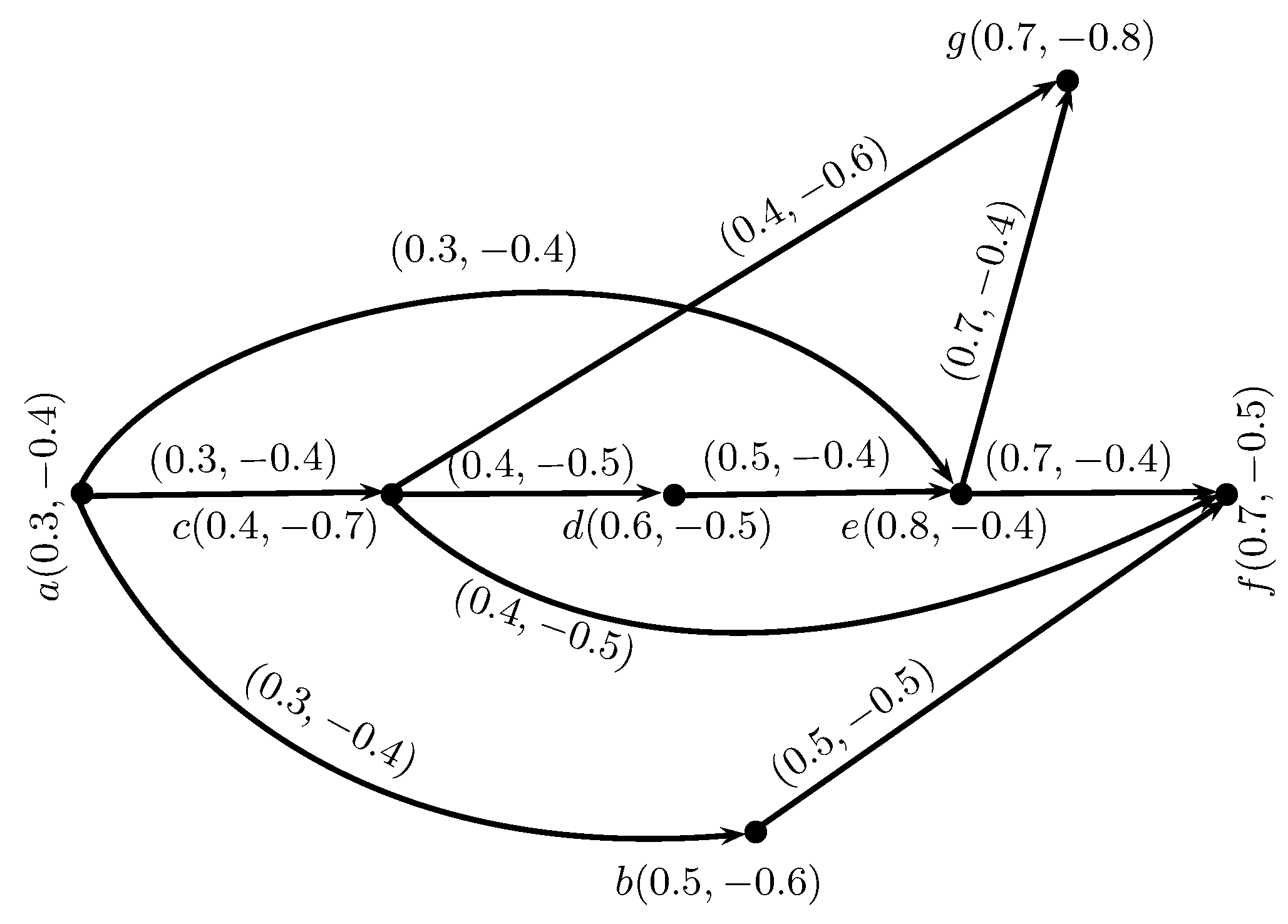
Example 1.
The bipolar fuzzy outneighborhood is given in Table 2.
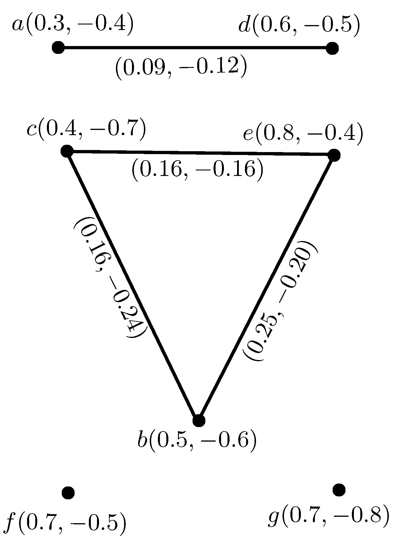
The bipolar fuzzy competition graph of the bipolar fuzzy digraph is shown in Figure 2.
Theorem 1.
Let G be a bipolar fuzzy graph, then adding a sufficient number of isolated vertices to G produces a bipolar fuzzy competition graph of some bipolar fuzzy digraph.
Proof.
Let be a bipolar fuzzy graph of the crisp graph where is a bipolar fuzzy set on the set of vertices X and is a bipolar fuzzy set on the set of edges E. Construct the bipolar fuzzy digraph as follows: Let be any two vertices of G such that or . Add a vertex ; remove the edge ; and draw directed edges from x and y to such that:
Continuing this process, we obtain a bipolar fuzzy digraph such that where I is the bipolar fuzzy set of isolated vertices added to G. ☐
3. Decision-Making Approach of Competition Graphs and the Extended TOPSIS Method Based on Bipolar Fuzzy Sets
We now present several applications of bipolar fuzzy competition graphs in food webs.
3.1. Bipolar Fuzzy Competition Graph in Food Webs
Food webs are the graphical representations of the natural interconnection of food chains between different species. Competition graphs arose in connection with an application to food webs. In a food web, vertices represent species, and there is a directed edge between two species x and y if y is a food for x. Bipolar fuzzy graphs are more realistic to represent the competition between species.
Let represent a bipolar fuzzy food web of a crisp food web in which vertices represent the species and if x preys on y. Bipolar fuzzy food webs can play an important role in investigating the flow of energy and the predator-prey relationship in the ecosystem. The bipolar fuzzy competition graph can be constructed from the bipolar fuzzy food web to study to what extent species compete for common prey. It is defined as: Let be a bipolar fuzzy food web. The bipolar fuzzy competition graph has the same vertices as , and there is an edge between two vertices x and y if and:
We present an algorithm that is used to calculate the strength of competition between species in an ecosystem.
Algorithm 1.
- Given any bipolar fuzzy food web.
- Construct the table of bipolar fuzzy in neighborhoods of all the species.
- Construct the bipolar fuzzy competition graph using the above definition.
- If for any two species x and y, then the strength of competition between x and y for common food is:
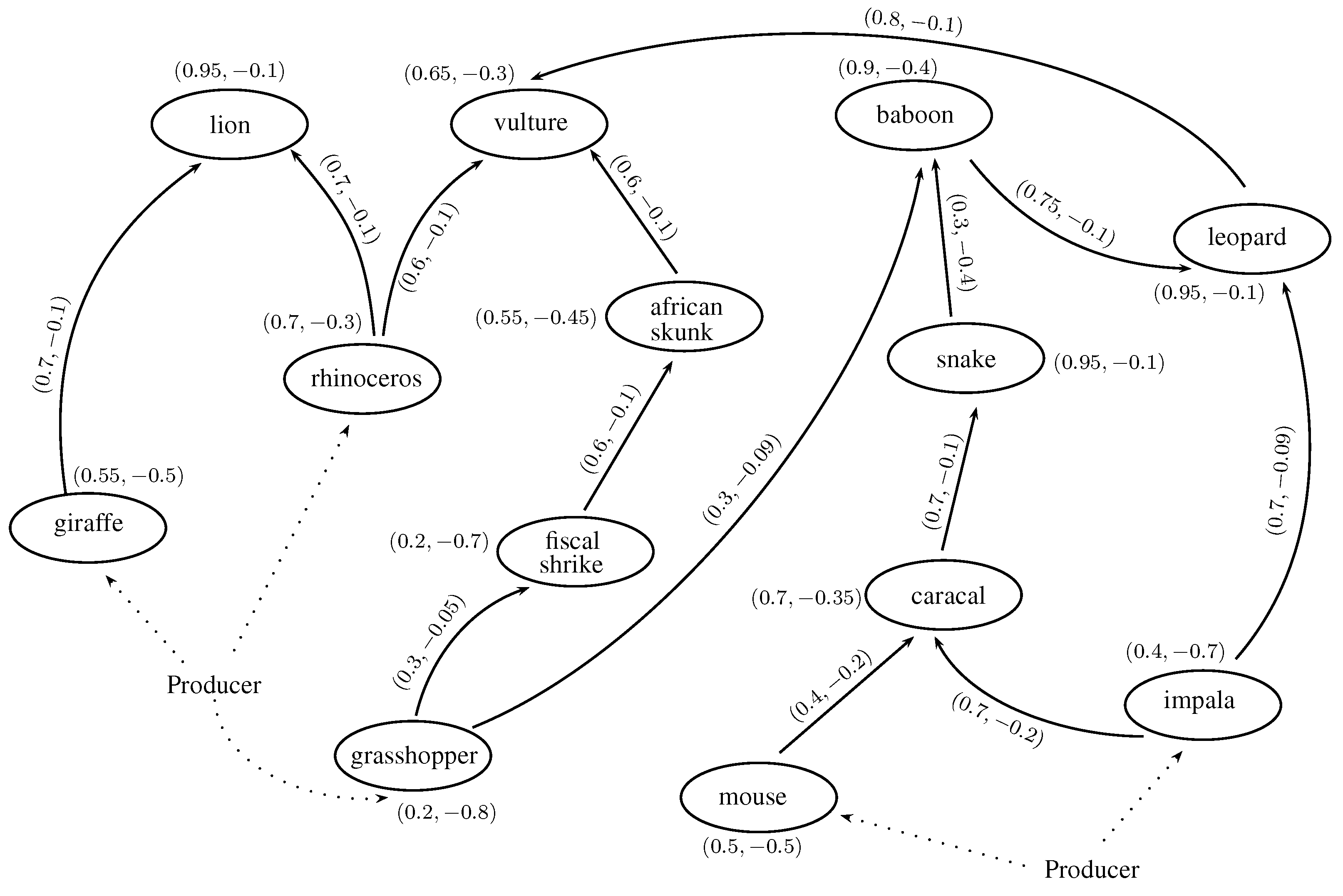
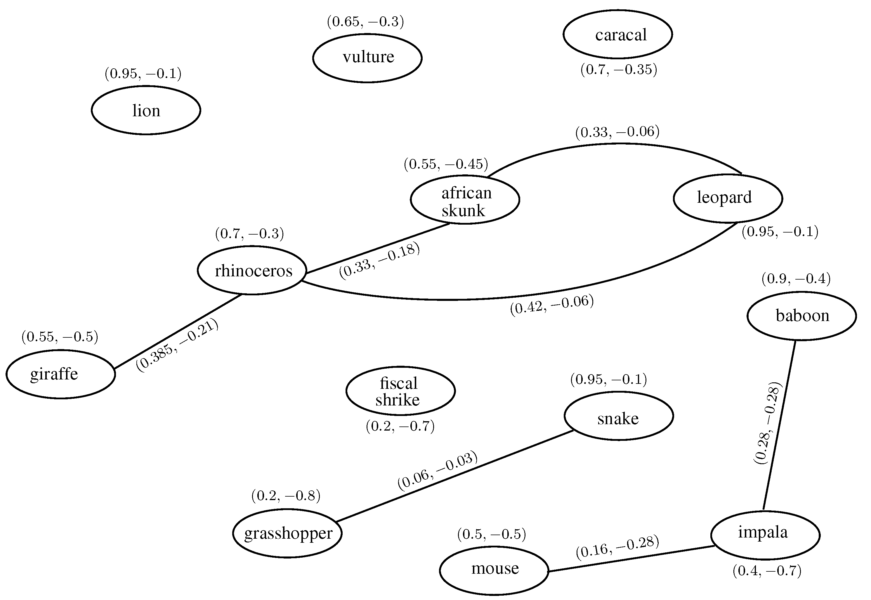
Consider the example of bipolar fuzzy food web of 13 species: giraffe, lion, vulture, rhinoceros, African skunk, fiscal shrike, grasshopper, baboon, leopard, snake, caracal, mouse and impala. The positive degree of membership of each species represents to what extent the species is strong according to its power and can defend itself to exist in the animal kingdom. The negative degree of membership of a species represents its weakness that it can be killed or dominated by other species. The bipolar fuzzy food web is shown in Figure 3.
The degree of membership of lion is , which shows that lion is strong in its kingdom according to hunting power and weak because a group of animals together can dominate a lion. The directed edge between giraffe and lion has degree of membership , which represents that a lion obtains energy from giraffe, and a giraffe is harmful for a lion because it can kill a lion with its long legs.
This is an acyclic bipolar fuzzy digraph. A bipolar fuzzy competition graph can be constructed to investigate the strength of competition between species for common food prey. The bipolar fuzzy in neighborhoods are given in Table 3.
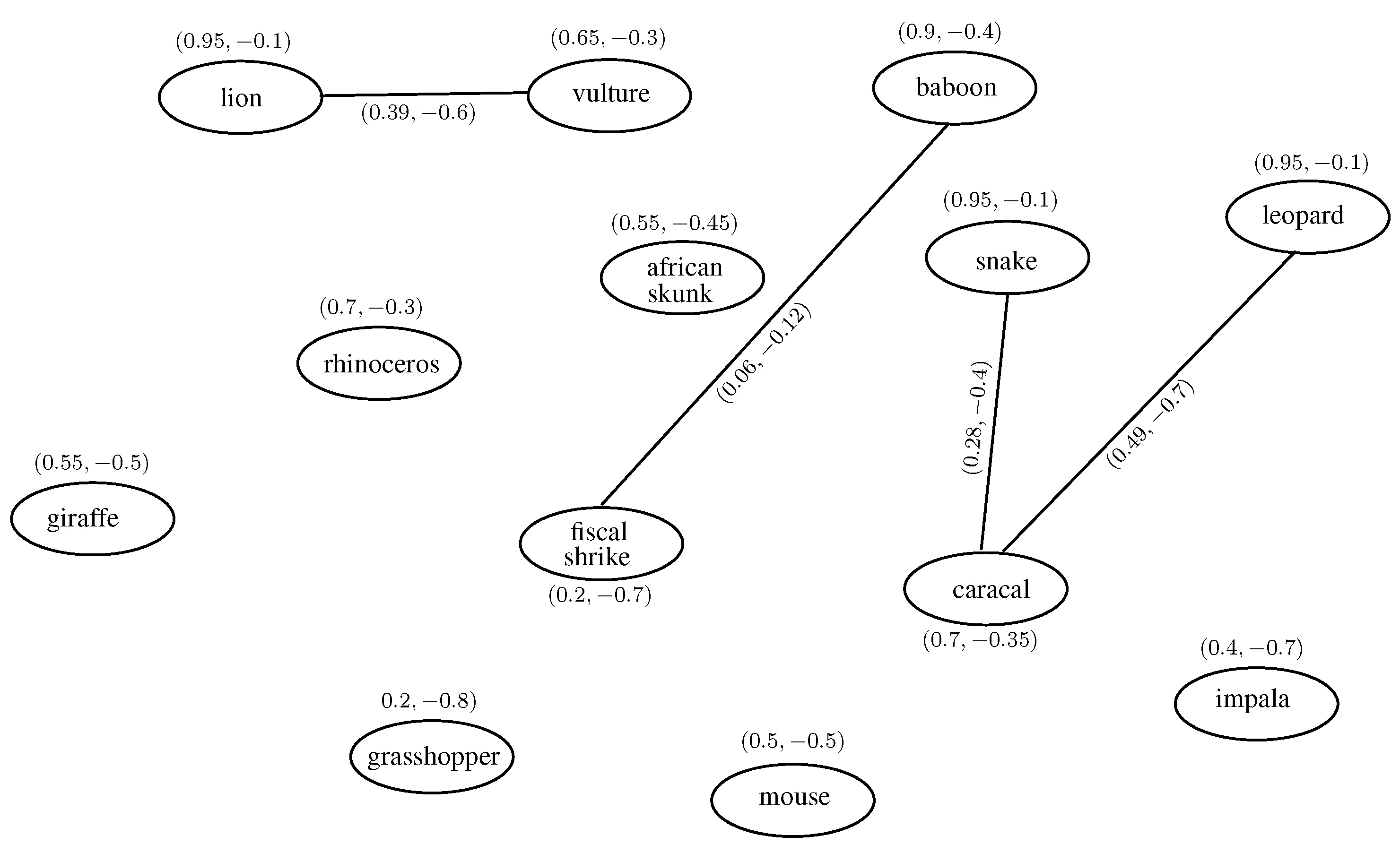
The bipolar fuzzy competition graph is shown in Figure 4. There is food competition between lion and vulture, fiscal shrike and baboon, snake and caracal, leopard and caracal. The membership value of the edge between two species represents the degree of the benefits and harm of common food.
The strength of competition between species x and y calculated using Formula (1) is given in Table 4.
According to Table 4, there is a strong competition between caracal and leopard for common food with respect to hunting powers and weaknesses.
3.2. Bipolar Fuzzy Common Enemy Graph
Bipolar common enemy graphs can be constructed from bipolar fuzzy food webs to study the strength of common enemies between species. It is defined as:
Let be a bipolar fuzzy food web. The bipolar fuzzy common enemy graph has the same set of species as , and there is an edge between two species x and y if , i.e., x and y has a common predator and:
We present the method of calculating the strength of common enemies between species in an ecosystem as an algorithm.
Algorithm 2.
- Given any bipolar fuzzy food web.
- Construct the table of bipolar fuzzy out neighborhoods of all the species.
- Construct the bipolar fuzzy competition graph using the above definition.
- If for any two species x and y, then the strength of competition between x and y for common food is:
Consider the example of a bipolar fuzzy food web of 13 species as shown in Figure 3. The bipolar fuzzy out neighborhoods are given in Table 5.
The bipolar fuzzy common enemy graph is shown in Figure 5. There are common enemies between giraffe and rhinoceros, rhinoceros and African skunk, rhinoceros and leopard, African skunk and leopard, grasshopper and snake, mouse and impala and baboon and impala. The positive membership value of the edge between two species represents the degree of energy both provide to common predator-enemy, and the negative degree of membership shows to what extent they can harm their common enemy.
3.3. Bipolar Fuzzy Competition Common Enemy Graph
Bipolar fuzzy competition common enemy graphs can be constructed from bipolar fuzzy food webs to study the relationship of common enemies, as well as competition for prey between species. It is defined as:
Let be a bipolar fuzzy food web. The bipolar fuzzy competition common enemy graph has same vertices as , and there is an edge between two vertices x and y if and , i.e., x and y have a common predator and a common prey where,
We depict our method of finding the strength of power of each species according to competition for common prey and common enemies as an algorithm.
Algorithm 3.
- Given any bipolar fuzzy food web.
- Construct the table of bipolar fuzzy out neighborhoods and bipolar fuzzy in neighborhoods of all the species.
- Construct the bipolar fuzzy competition graph using the above definition.
- If and for any two species x and y, then calculate the degree of each species x,
- The strength of the power of each species x is
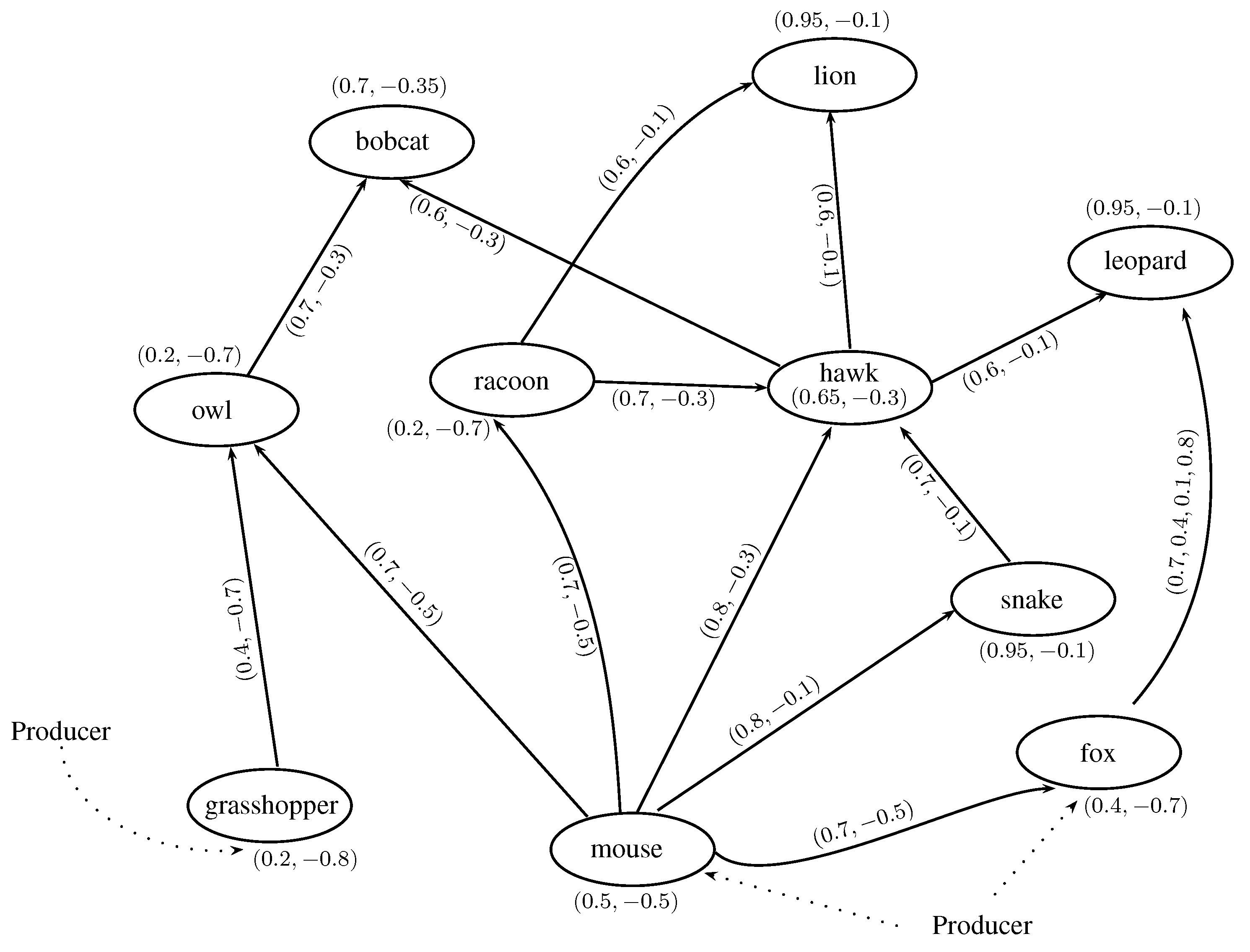
Consider the example of a bipolar fuzzy food web of 10 species as shown in Figure 6. The description of the degrees of membership of vertices and directed edges is the same as in Figure 3.
The bipolar fuzzy out neighborhoods and bipolar fuzzy in neighborhoods are given in Table 7.
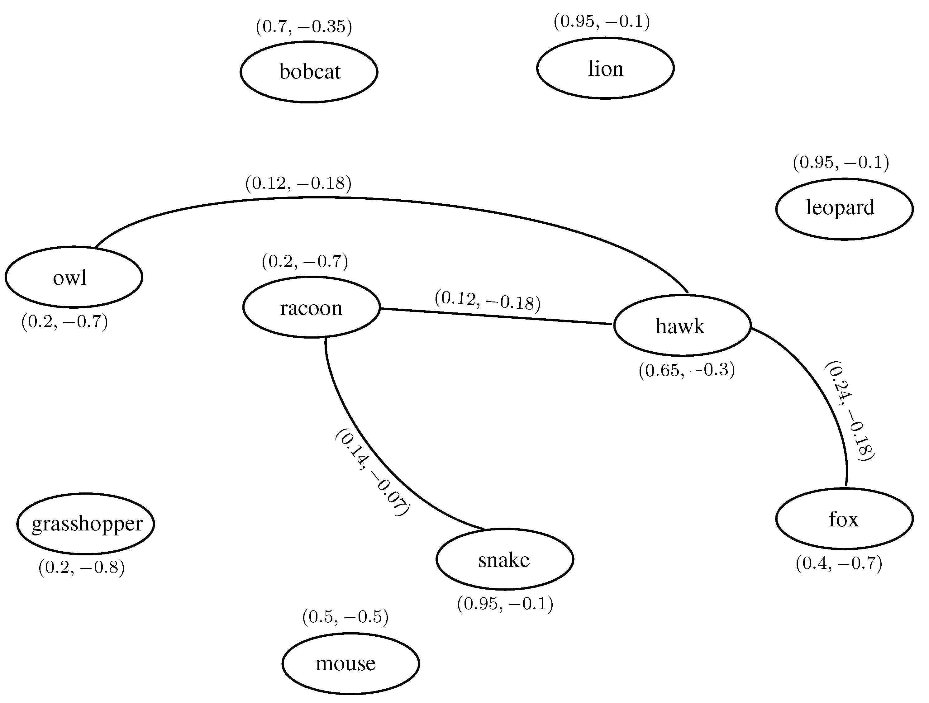
The bipolar fuzzy competition common enemy graph is shown in Figure 7.
The strength of power of each species according to food competition and common enemies is calculated in Table 8, which depicts that hawk is the most powerful animal in this bipolar fuzzy food web.
3.4. Bipolar Fuzzy Niche Graph
Niche graphs are important to study the behavior of species in ecological networks. Since all the species have different characteristics with respect to each other, therefore the bipolar fuzzy niche graphs can play a substantial role to study ecological networks more precisely. A bipolar fuzzy niche graph is defined as:
Let be a bipolar fuzzy food web. The bipolar fuzzy niche graph has the same vertices as , and there is an edge between two vertices x and y if or , i.e., x and y have a common predator or a common prey where,
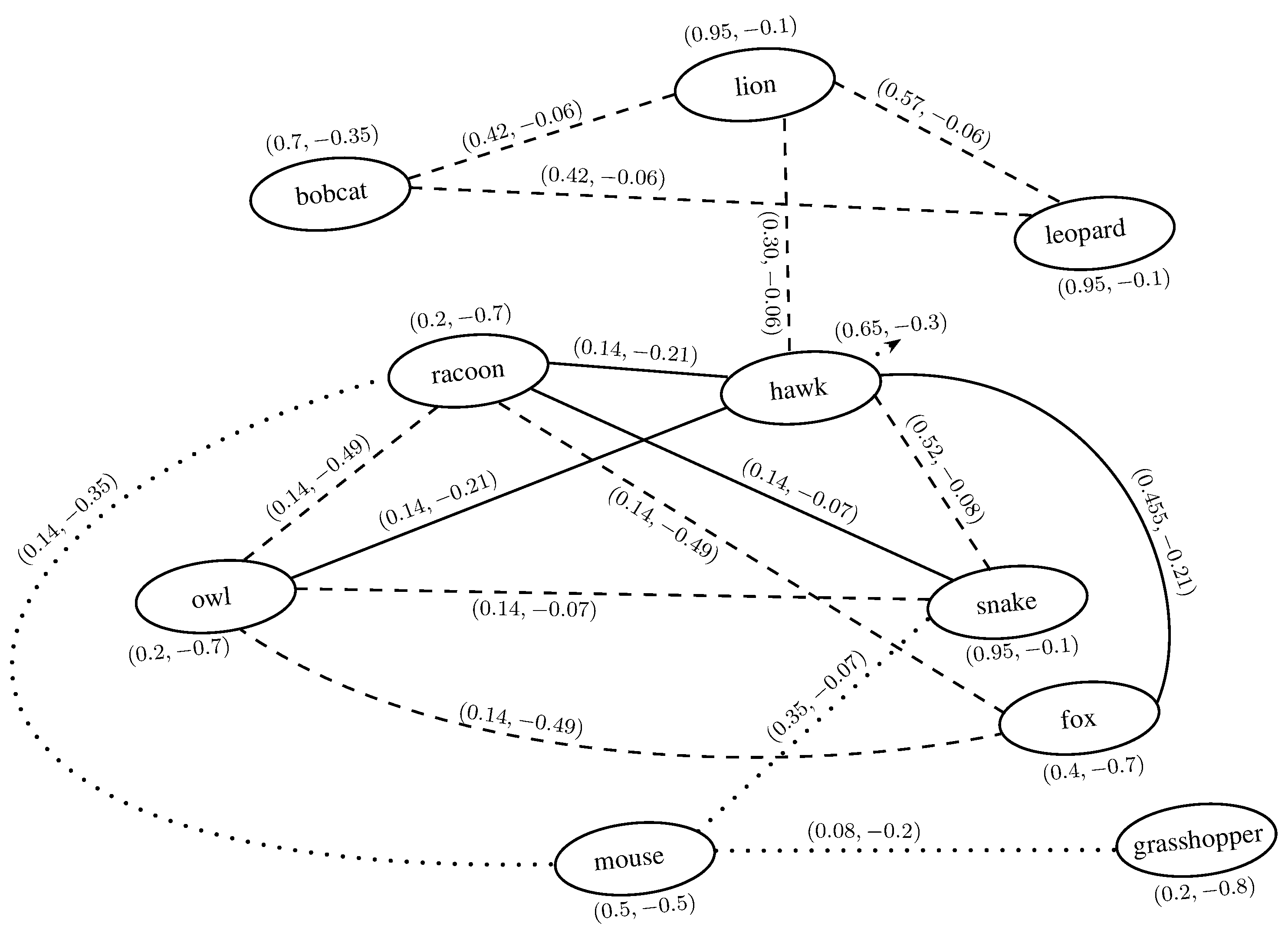
The bipolar fuzzy niche graph of Figure 6 is shown in Figure 8. The edge between species that have only common prey is represented by dashed lines; dotted lines represent the species relationship having only common enemies; and solid lines represent the species that have both common prey and common enemies.
3.5. Multi-Criteria Decision Making Method to Minimize the Side Effects of Dental Treatments
Tooth diseases are very common nowadays due to the increasing demand for unhealthy food. The problem affecting millions of people the most is tooth decay. Our mouth is a ground for good and bad bacteria. People are not used to thinking of teeth as living organs and tissues. There are various treatments to prevent cavities, gum disease, toothaches, missing teeth, etc. However, on the other hand, it is roughly estimated that almost 70% of human diseases are indirectly or directly due to intervention in the tooth structures. This includes: teeth filling with various metallic and non-metallic materials, root canals, dental bridges, teeth implants, metal braces, crowns and caps, dentures, gum surgery, teeth veneers, composite bridges, etc. Bipolar fuzzy sets can be used to detect the diseases caused by various treatments considering the benefits of the treatment. If are the alternative materials and are the side effects corresponding to each alternative, then the procedure for the selection of a suitable treatment with minimum danger is given in Algorithm 4.
Algorithm 4. Bipolar fuzzy extended TOPSIS method based on entropy weights.
- Input the n number of alternative materials .
- Input the side effects corresponding to each alternative.
- Input the bipolar fuzzy decision matrix where represents the degree of membership of alternative with respect to criteria . The positive degree of membership represents the degree of side effect for implementing , and the negative degree of membership represents the degree of benefit of material .
- Determine the criteria weight (information entropy) of each side effect , , using Formula (3).where is a constant such that .
- Calculate the degree of divergence of each side effect using Equation (4).
- Calculate the entropy weights corresponding to each criterion as given in Equation (5):
- Construct the weighted bipolar fuzzy decision matrix where, for each , is defined in Equation (6).
- Calculate the relative closeness degree of each alternative using Equation (11).
- Arrange all the alternatives in descending order according to the relative closeness degree.
We now describe an example of teeth replacement alternatives to illustrate Algorithm 4.
Replacement of a Missing Tooth
A person may face the problem of missing teeth due to gum disease, tooth decay, injury, by birth or inherited disorder. With the passage of time, missing teeth can cause various health issues including poor nutrition and chewing problems. One missing tooth can weaken the jaw structure. People often visit dentists for replacement of missing teeth. There are various alternative replacement options for a missing tooth such as a traditional bridge, denture, cantilever bridge, resin bonding, teeth implant, etc. The benefits and side effects of teeth replacements vary in patients. Every person has different skin and teeth sensitivities; therefore, the side effects of dental treatments are not constant in patients. Consider the example of a person X who wants a teeth replacement treatment. The side effects and benefits of alternative treatments with respect to person X are shown in Table 9. The description of the degree of membership of each criterion (side effect) is shown in Table 10.
Denote each side effect by as given in Table 11. By taking , the calculations of entropy wights are given in Table 11.
The weighted bipolar fuzzy decision matrix is given in Table 12.
The bipolar fuzzy positive and negative ideal solutions are given in Table 13.
The distance measures and relative closeness degree of each alternative measure are given in Table 14.
Arranging the alternatives in decreasing order according to relative closeness degree, we conclude that a traditional bridge is the best option for replacement of missing teeth.
A View of Bipolar Fuzzy Extended TOPSIS
Multi-criteria decision-making (MCDM) is a procedure to make an ideal decision that has the highest level of of achievement from a set of alternatives that are characterized regarding various conflicting criteria. TOPSIS methods are the most effective and favorable methods to solve MCDM problems. To deal with uncertainty and incomplete information, fuzziness, intuitionistic fuzziness and neutrosophic sets have been utilized successfully in TOPSIS methods for solving MCDM problems. However, in many cases, the given information is bipolar in nature. Recently, a bipolar fuzzy TOPSIS method for the suitable selection of objects was discussed in [5]. However, in this method, the weights are chosen arbitrarily, which can be changed according to the choice of decision-makers. The chosen weights may be irrelevant for the given information, which can effect the outcomes of decision-making. Therefore, it is necessary to calculate weights according to the given information. In our method, we have discussed the process for calculating entropy weights from given bipolar fuzzy information. It gives more suitable decisions as compared to the previous methods discussed in the literature.
4. Conclusions
Bipolar fuzzy graphs play a vital role in many research domains and give more precision, flexibility and compatibility to the system as compared to the classical and fuzzy models. A bipolar fuzzy set is an extension of a fuzzy set with the additional possibility to represent bipolar uncertainty and vagueness that exist in real-world situations. In this paper, we have presented the procedure of the bipolar fuzzy extended TOPSIS method based on entropy weights in the form of an algorithm. For illustration, we have applied this method to a real-life problem in dentistry. We have also discussed applications of bipolar fuzzy competition graphs and proved that every bipolar fuzzy graph is a bipolar fuzzy competition graph of some bipolar fuzzy digraph. We have presented four different variations of bipolar fuzzy competition graphs in food webs and studied the strength of competition between species. We have also studied the process for calculating the strength of competition with certain algorithms.
5. Future Work
Author Contributions
M.S., M.A. and F.Z. conceived of and designed the experiments. M.S. and F.Z. wrote the paper.
Conflicts of Interest
The authors declare no conflict of interest.
References
- Hwang, C.L.; Yoon, K. Multiple attribute decision-making-methods and applications. In A State of the Art Survey; Springer: New York, NY, USA, 1981. [Google Scholar]
- Chen, C.-T. Extension of the TOPSIS for group decision-making under fuzzy environment. Fuzzy Sets Syst. 2000, 114, 1–9. [Google Scholar] [CrossRef]
- Hung, C.-C.; Chen, L.-H. A fuzzy TOPSIS decision-making model with entropy weright under intuitionistic fuzzy environment. In Proceedings of the International MultiConference of Engineers and Computer Scientists, Hong Kong, China, 18–20 March 2009; Volume 1. [Google Scholar]
- Li, D.-F.; Nan, J.-X. Extension of the TOPSIS for multi-attribute group decision-making under atanassov IFS environments. Int. J. Fuzzy Syst. Appl. 2011, 4, 47–61. [Google Scholar] [CrossRef]
- Alghamd, M.A.; Alshehri, N.O.; Akram, M. Multi-criteria decision-making methods in bipolar fuzzy environment. Int. J. Fuzzy Syst. 2018, 20, 2057–2064. [Google Scholar] [CrossRef]
- Garg, H.; Gagandeep, K. Extended TOPSIS method for multi-criteria group decision-making problems under cubic intuitionistic fuzzy environment. Sci. Iran. 2018. [Google Scholar] [CrossRef]
- Garg, H.; Kumar, K. Improved possibility degree method for ranking intuitionistic fuzzy numbers and their application in multiattribute decision-making. Granul. Comput. 2018, 1–11. [Google Scholar] [CrossRef] [Green Version]
- Garg, H.; Kumar, K. Group Decision Making Approach Based on Possibility Degree Measures and the Linguistic Intuitionistic Fuzzy Aggregation Operators Using Einstein Norm Operations. J. Multiple-Valued Logic Soft Comput. 2018, 31, 209–235. [Google Scholar]
- Kumar, K.; Garg, H. Connection number of set pair analysis based TOPSIS method on intuitionistic fuzzy sets and their application to decision-making. Appl. Intell. 2018, 48, 2112–2119. [Google Scholar] [CrossRef]
- Kumar, K.; Garg, H. TOPSIS method based on the connection number of set pair analysis under interval-valued intuitionistic fuzzy set environment. Comput. Appl. Math. 2018, 37, 1319–1329. [Google Scholar] [CrossRef]
- Garg, H. A new improved score function of an interval-valued Pythagorean fuzzy set based TOPSIS method. Int. J. Uncertain. Quantif. 2017, 7, 463–474. [Google Scholar] [CrossRef]
- Bashir, Z.; Rashid, T.; Watróbski, J.; Salabun, W.; Malik, A. Hesitant probabilistic multiplicative preference relations in group decision-making. Appl. Sci. 2018, 8, 398. [Google Scholar] [CrossRef]
- Faizi, S.; Rashid, T.; Salabun, W.; Zafar, S.; Watróbski, J. Decision making with uncertainty using hesitant fuzzy sets. Int. J. Fuzzy Syst. 2018, 20, 93–103. [Google Scholar] [CrossRef]
- Faizi, S.; Salabun, W.; Rashid, T.; Watróbski, J.; Zafar, S. Group decision-making for hesitant fuzzy sets based on characteristic objects method. Symmetry 2017, 9, 136. [Google Scholar] [CrossRef]
- Jankowski, J.; Salabun, W.; Watróbski, J. Identification of a multi-criteria assessment model of relation between editorial and commercial content in web systems. In Multimedia and Network Information Systems; Springer: Cham, Switzerland, 2017; pp. 295–305. [Google Scholar]
- Akram, M.; Shumaiza, S.F. Decision-Making with Bipolar Neutrosophic TOPSIS and Bipolar Neutrosophic ELECTRE-I. Axioms 2018, 7, 33. [Google Scholar] [CrossRef]
- Zadeh, L.A. Fuzzy sets. Inf. Control 1965, 8, 338–353. [Google Scholar] [CrossRef] [Green Version]
- Zhang, W.-R. Bipolar fuzzy sets and relations: A computational framework for cognitive modeling and multiagent decision analysis. In Proceedings of the First International Joint Conference of the North American Fuzzy Information Processing Society Biannual Conference, San Antonio, TX, USA, 18–21 December 1994; pp. 305–309. [Google Scholar]
- Zadeh, L.A. Similarity relations and fuzzy orderings. Inf. Sci. 1971, 3, 177–200. [Google Scholar] [CrossRef]
- Kaufmann, A. Introduction la Thorie des Sous-Ensembles Flous l’Usage des Ingnieurs (Fuzzy Sets Theory); Masson: Paris, France, 1975. [Google Scholar]
- Rosenfeld, A. Fuzzy Sets and Their Applications; Academic Press: New York, NY, USA, 1975; pp. 77–95. [Google Scholar]
- Samanta, S.; Pal, M. Fuzzy k-competition and p-competition graphs. Fuzzy Inf. Eng. 2013, 2, 191–204. [Google Scholar] [CrossRef]
- Al-shehri, N.O.; Akram, M. Bipolar fuzzy competition graphs. Ars Comb. 2015, 121, 385–402. [Google Scholar]
- Akram, M. Bipolar fuzzy graphs. Inf. Sci. 2011, 181, 5548–5564. [Google Scholar] [CrossRef]
- Akram, M. Bipolar fuzzy graphs with applications. Knowl. Based Syst. 2013, 39, 1–8. [Google Scholar] [CrossRef]
- Akram, M.; Sarwar, M. Bipolar fuzzy circuits with applications. J. Intell. Fuzzy Syst. 2016, 34, 547–558. [Google Scholar]
- Sarwar, M.; Akram, M. Novel concepts bipolar fuzzy competition graphs. J. Appl. Math. Comput. 2016, 54, 511–547. [Google Scholar] [CrossRef]
- Cohen, J.E. Interval Graphs and Food Webs: A Finding and a Problem. Available online: http://lab.rockefeller.edu/cohenje/assets/file/014.1CohenIntervalGraphsFoodWebsRAND1968.pdf (accessed on 22 September 2018).
- Scott, D.D. The competition common-enemy graph of a digraph. Discret. Appl. Math. 1987, 17, 269–280. [Google Scholar] [CrossRef]
- Mordeson, J.N.; Nair, P.S. Fuzzy Graphs and Fuzzy Hypergraphs; Springer: Berlin / Heidelberg, Germany, 2000. [Google Scholar]
- Rosen, K.H. Discrete Mathematics and Its Applications, 7th ed.; McGraw-Hill Education: New York, NY, USA, 2012. [Google Scholar]
- Samanta, S.; Akram, M.; Pal, M. m-step fuzzy competition graphs. J. Appl. Math. Comput. 2015, 47, 461–472. [Google Scholar] [CrossRef]
- Cable, C. Niche Graphs. Discret. Appl. Math. 1989, 23, 231–241. [Google Scholar] [CrossRef]
- Garg, H. Linguistic pytagorean fuzzy sets and its applications in multi-attribute decision-making preocess. Int. J. Intell. Syst. 2018, 33, 1234–1263. [Google Scholar] [CrossRef]
- Garg, H. Hesitant pythagorean fuzzy sets and their aggregation operators in multiple-attribute decision-making. Int. J. Uncertain. Quantif. 2018, 8, 267–289. [Google Scholar] [CrossRef]
- Garg, H. New logarithmic operational laws and their aggregation operators for pythagorean fuzzy set and their applications. Int. J. Fuzzy Syst. 2018. [Google Scholar] [CrossRef]
Figure 1.
Bipolar fuzzy digraph.

Figure 2.
Bipolar fuzzy competition graph.

Figure 3.
Bipolar fuzzy web.

Figure 4.
Bipolar fuzzy competition graph.

Figure 5.
Quadripolar fuzzy common enemy graph.

Figure 6.
Bipolar fuzzy food web.

Figure 7.
Bipolar fuzzy competition common enemy graph.

Figure 8.
Quadripolar fuzzy niche graph.


Table 1.
Adjacency matrix.
| X | a | b | c | d | e | f | g |
|---|---|---|---|---|---|---|---|
| a | |||||||
| b | |||||||
| c | |||||||
| d | |||||||
| e | |||||||
| f | |||||||
| g |
Table 2.
Bipolar fuzzy inneighborhood.
| ∅ | |
| ∅ |
Table 3.
The bipolar fuzzy in neighborhoods.
| Species | Is a Species |
|---|---|
| giraffe | |
| lion | |
| rhinoceros | |
| vulture | |
| African skunk | |
| fiscal shrike | |
| grasshopper | |
| baboon | |
| leopard | |
| snake | |
| caracal | |
| mouse | |
| impala |
Table 4.
Strength of competition between species.
| Species | Strength of Competition | Species | Strength of Competition |
|---|---|---|---|
| lion, vulture | shrike, baboon | ||
| snake, caracal | caracal, leopard |
Table 5.
Bipolar fuzzy out neighborhoods.
| Species | Is a Species |
|---|---|
| giraffe | |
| lion | ∅ |
| rhinoceros | |
| vulture | ∅ |
| African skunk | |
| fiscal shrike | |
| grasshopper | |
| baboon | |
| leopard | |
| snake | |
| caracal | |
| mouse | |
| impala |
Table 6.
Strength of common enemies between species.
| giraffe, rhinoceros | grasshopper, snake | ||
| rhinoceros, African skunk | impala, baboon | ||
| African skunk, leopard | mouse, impala | ||
| rhinoceros, leopard | - | - |
Table 7.
Bipolar fuzzy out neighborhoods and in neighborhoods.
| x Is a Species | and |
|---|---|
| grasshopper | grasshopper, grasshopper)= |
| owl | owl)= owl |
| bobcat | bobcat)=, bobcat |
| lion | lion)=, lion |
| leopard | leopard)=, leopard |
| raccoon | raccoon)= raccoon |
| hawk | hawk)= hawk |
| mouse | mouse, mouse)= |
| fox | fox, fox |
| snake | snake, snake |
Table 8.
Strength of competition between species.
| Species | Degree of Each Species | Power in Food Web |
|---|---|---|
| owl | ||
| raccoon | 0.755 | |
| hawk | 1.01 | |
| snake | 0.605 |
Table 9.
Bipolar fuzzy decision matrix.
| Alternatives | Disadvantages and Benefits | ||||||
|---|---|---|---|---|---|---|---|
| Affordable | Bone Infection | Damage to Natural Teeth | Long Lasting | Toothache | Risk of Tooth Decay | Gum Disease | |
| Traditional Bridge | () | ||||||
| Cantilever Bridge | |||||||
| Resin Bonded | |||||||
| Removable Denture | |||||||
| Teeth Implant | |||||||
Table 10.
Bipolar fuzzy decision matrix.
| Criteria | Positive Degree of Membership | Negative Degree of Membership |
|---|---|---|
| Affordable | Replacement option is affordable | Replacement option is expensive |
| Bone Infection | Infection causes jawbone loss | Prevents the risk of jawbone loss |
| Damage to Natural Teeth | Damage to abutting healthy teeth | Prevents the future decay and shifting of healthy adjacent teeth |
| Long Lasting | Restoration can collapse and needs to be replaced early | Treatment will last long |
| Toothache | Treatment causes toothache with the passage of time | Treatment prevents risk of toothache |
| Risk of Tooth Decay | Tooth decay under the replacement | Good dentistry prevents tooth loss |
| Gum Disease | Replacement causes gum infections and diseases | Prevents the risk of gum infection |
Table 11.
Entropy weights.
| Calculated Values | Disadvantages and Benefits | ||||||
|---|---|---|---|---|---|---|---|
| Affordable | Bone Infection | Damage to Natural Teeth | Long Lasting | Toothache | Risk of Tooth Decay | Gum Disease | |
| 0.267 | 0.272 | 0.293 | 0.285 | 0.352 | 0.261 | 0.32 | |
| 0.733 | 0.728 | 0.707 | 0.715 | 0.648 | 0.739 | 0.68 | |
| 0.148 | 0.147 | 0.143 | 0.14 | 0.131 | 0.149 | 0.137 | |
Table 12.
Weighted bipolar fuzzy decision matrix.
| Criteria | Alternatives | ||||
|---|---|---|---|---|---|
| Traditional Bridge | Cantilever Bridge | Resin Bonded | Removable Denture | Teeth Implant | |
Table 13.
Bipolar fuzzy positive and negative ideal solutions.
| 0.03 | 0.015 | 0.057 | 0.056 | 0.066 | 0.045 | 0.014 | |
| −0.084 | |||||||
| 0.133 | 0.118 | 0.129 | 0.112 | 0.092 | 0.134 | 0.11 | |
Table 14.
Distance measures and relative closeness degree.
| Calculated Values | Traditional Bridge | Cantilever Bridge | Resin Bonded | Removable Denture | Teeth Implant |
|---|---|---|---|---|---|
| 2.3018 | 2.2634 | 2.0521 | 1.9615 | 2.2648 | |
| 2.0314 | 1.9862 | 1.8164 | 1.7372 | 2.002 | |
| 0.4688 | 0.5326 | 0.4695 | 0.4697 | 0.4692 |
© 2018 by the authors. Licensee MDPI, Basel, Switzerland. This article is an open access article distributed under the terms and conditions of the Creative Commons Attribution (CC BY) license (http://creativecommons.org/licenses/by/4.0/).
Share and Cite
MDPI and ACS Style
Sarwar, M.; Akram, M.; Zafar, F. Decision Making Approach Based on Competition Graphs and Extended TOPSIS Method under Bipolar Fuzzy Environment. Math. Comput. Appl. 2018, 23, 68. https://doi.org/10.3390/mca23040068
AMA Style
Sarwar M, Akram M, Zafar F. Decision Making Approach Based on Competition Graphs and Extended TOPSIS Method under Bipolar Fuzzy Environment. Mathematical and Computational Applications. 2018; 23(4):68. https://doi.org/10.3390/mca23040068
Chicago/Turabian StyleSarwar, Musavarah, Muhammad Akram, and Fariha Zafar. 2018. "Decision Making Approach Based on Competition Graphs and Extended TOPSIS Method under Bipolar Fuzzy Environment" Mathematical and Computational Applications 23, no. 4: 68. https://doi.org/10.3390/mca23040068