Modified Auxiliary Equation Method versus Three Nonlinear Fractional Biological Models in Present Explicit Wave Solutions

Abstract

In this article, we present a modified auxiliary equation method. We harness this modification in three fundamental models in the biological branch of science. These models are the biological population model, equal width model and modified equal width equation. The three models represent the population density occurring as a result of population supply, a lengthy wave propagating in the positive x-direction, and the simulation of one-dimensional wave propagation in nonlinear media with dispersion processes, respectively. We discuss these models in nonlinear fractional partial differential equation formulas. We used the conformable derivative properties to convert them into nonlinear ordinary differential equations with integer order. After adapting, we applied our new modification to these models to obtain solitary solutions of them. We obtained many novel solutions of these models, which serve to understand more about their properties. All obtained solutions were verified by putting them back into the original equations via computer software such as Maple, Mathematica, and Matlab.

1. Introduction

Since the emergence of humanity, people have taken a great interest in understanding natural phenomena, beginning from fire, lightning, thunder, earthquakes, and volcanoes, ranging all to way to the nano-particle. In the beginning of the 18th century, many scientists demonstrated an interest in studying these phenomena. The development of these studies continued until the middle of the 19th century. Partial differential equations (PDEs) became an essential tool for studying other branches of science, and many phenomena have been explained using PDEs. Many techniques for solving PDEs have been developed by scientists and researchers in their efforts to explain these phenomena. Many methods have been derived to obtain exact and approximate solutions of these models. The most important results in determining explicit solutions of nonlinear partial differential equations (NLPDEs) were derived in [1]. These types of methods are best known as continuous symmetry transformation groups [2,3,4,5,6]. At present, we use computer software (e.g., Maple, Mathematica) to make this kind of transformation. Since the 20th century, the investigation of the partial differential equation has become an independent field. Partial differential equations have been applied to the study of many phenomena in different fields, such as sound, heat, electrostatics, electrodynamics, fluid dynamics, elasticity, quantum mechanics, solid state physics, fluid mechanics, hydrodynamics, optics, plasma physics, chemical kinetics, biological phenomena, and more. It is known that there exist various analytic solution methods for NPDEs [7,8,9,10,11,12,13,14,15,16,17,18,19,20,21]. However, in the general case, there is no central theory for NPDEs. There is no unified method that can be applied to all types of nonlinear PDEs. For these reasons, we have to discover new methods for solving these kinds of models, and cannot just make modifications to methods that were discovered more than 100 years ago. Recently, fractional nonlinear partial differential equations have played an important role in the representation of many phenomena. Fractional rule half differential equations are increasingly chronic in accordance with mannequin problems between fluid flow, pay up and vile areas over the application. Fractional derivatives grant spiffy arms for the story on devotion or ancestral houses concerning various substances then processes. Half-order derivatives and integrals prove according to lie more useful for the method concerning sure electrochemical problems than the first-rate models. Fractional differentiation and integration operators are additionally chronic for extensions about the pervasion then suspense equations. Many researchers tried in conformity with finding out extra properties expecting that form of derivatives. They discovered partially about methods in accordance with changing the nonlinear fractional half differential equations among everyday differential equation together with integer order. For more important points in relation to these types of derivatives, we refer the reader to References [22,23,24,25,26,27,28,29]. In this paper, we use conformable derivative properties and apply them to three nonlinear biological models. These models are a fractional biological population model [30,31,32,33,34], a fractional equal width equation [35,36,37,38], and a fractional modified equal width equation [39,40,41,42], respectively.

The rest of this research paper is organized as follows: In Section 2, we give the headlines of the modified auxiliary equation method. In Section 3, we employ a novel computation to get the solitary solutions of the fractional biological population model, fractional equal width equation, and fractional modified equal width equation. In Section 4, we study the obtained solutions and their novelty with the previous method. In Section 5, we represent the conclusion of this study.

2. Fundamental Steps of the New Technique

Consider a nonlinear partial differential equation (NLPDE) with the following form:

$$F(u,u_x,u_t,u_{xx},u_{tt},\dots )=0,$$

(1)

where F is a polynomial in $u(x,t)$ and its partial derivatives in which the highest-order derivatives and nonlinear terms are involved. In the following, we give the steps of this method:

Step 1. Using the wave transformation:

$$u(x,t)=u(\theta ),\mathrm{where}[\theta =x+y+ct].$$

Using this transformation on (1), we convert the nonlinear partial differential equation into an ordinary differential equation with the following form:

$$f(u,u^{\prime },u^{″},\cdots )=0.$$

(2)

Step 2. Suppose that the solutions of ODE (2) have the following form:

$$u(\theta )=\sum _{i=1}^N{a}_i{K}^{if(\theta )}+a_0+\sum _{i=1}^N{b}_i{K}^{-if(\theta )},$$

(3)

where $(a_i,a)$ are arbitrary constants that will be determined later, while $f(\theta )$ satisfies the following ODE:

$$f^{\prime }(\theta )=\frac{1}{ln(a)}(\alpha K^{-f(\theta )}+\beta +\sigma K^{f(\theta )}).$$

(4)

Step 3. Determine the positive integer N in Equation (3) by balancing the highest-order derivatives and the nonlinear terms.

Step 4. Substituting Equations (3) and (4) into Equation (2) and collecting all the terms of the same power $(K^{if(\theta )})$ where $(i=-N,\cdots ,N)$ and equating them to zero, we get a system of algebraic equations that can be solved by Maple or Mathematica to get the values of $a_i,b_i$, and $(\alpha ,\beta ,\sigma )$.

Step 5. Substituting these values and the solutions of Equation (4) into Equation (3), we obtain the exact solutions of Equation (1).

3. Applications

In this part, we apply a novel computational method to two fractional models.

• Fractional biological population model:
  This model describes population dynamics. It also gives a simple example of how complex interactions and processes work. The model has the following form:

  $$\begin{array}{c}\hfill D_t^{\vartheta }u=D_{xx}^{2\vartheta }{u}^2+D_{yy}^{2\vartheta }{u}^2+\lambda (u^2-s),0<\vartheta <1,\end{array}$$

  (5)

  where u impersonates the population density and $\lambda (u^2-s)$ constitutes the population changes because of deaths and births.
• Fractional equal width equation:
  This model is usually used to describe complex physical phenomena in various fields, and has the following formula:

  $$\begin{array}{c}\hfill D_t^{\vartheta }u+2hu{D}_x^{\vartheta }u-r{D}_{xxt}^{3\vartheta }u=0,0<\vartheta <1,\end{array}$$

  (6)

  where $[h,r]$ are arbitrary constants.
• Fractional modified equal width equation:
  This model refers to the replica of one-dimensional wave propagation in nonlinear form with dispersion processes, and has the following formula:

  $$\begin{array}{c}\hfill D_t^{\vartheta }u+h{u}^2{D}_x^{\vartheta }u-r{D}_{xxt}^{3\vartheta }u,0<\vartheta <1,\end{array}$$

  (7)

  where $[h,r]$ are arbitrary constants.

Applying the conformable derivative definition and its properties to Equations (5) and (7) in respective order $[u(x,y,t)=u(\theta )\&\theta =\mu \frac{x^{\kappa }}{\kappa }+i\mu \frac{y^{\kappa }}{\kappa }+\frac{c{t}^{\kappa }}{\kappa }]$ & $[u(x,t)=u(\theta )\&\theta =\frac{x^{\kappa }}{\kappa }+\frac{c{t}^{\kappa }}{\kappa }]$, we transform the fractional PDE into an integer order ODE in the following order:

$$\begin{array}{c}\hfill c{u}^{\prime }-\lambda u^2+\lambda s=0,\end{array}$$

(8)

$$\begin{array}{c}\hfill cu+h{u}^2-rc{u}^{″}=0,\end{array}$$

(9)

$$\begin{array}{c}\hfill cu+\frac{h}{3}{u}^3-rc{u}^{″}=0.\end{array}$$

(10)

We balanced the terms in Equations (8)–(10) to get the balance value of each of them, obtaining the value of balance equal to one in all of them. According to the novel method, the general solution of Equations (8) and (10) is in the following form:

$$\begin{array}{c}\hfill u(\theta )=a_0+a_1{K}^{f(\theta )}+b_1{K}^{-f(\theta )},\end{array}$$

(11)

while the general solution of Equation (9) is in the next form:

$$\begin{array}{c}\hfill u(\theta )=a_0+a_1{K}^{f(\theta )}+a_2{K}^{2f(\theta )}+b_1{K}^{-f(\theta )}+b_2{K}^{-2f(\theta )}.\end{array}$$

(12)

3.1. Fractional Biological Population Model

Substitute Equation (11) and its derivatives into Equation (8). Collect all coefficients of the same terms for $K^{f(\theta )}$. Equating them to zero, we obtain system of algebraic equations. Solving this system via any computer software (e.g., Maple, Mathematica), we obtain:

$$a_0\to \frac{\beta \sqrt{s}}{\sqrt{{\beta }^2-4\alpha \sigma }},a_1\to 0,b_1\to \frac{2\alpha \sqrt{s}}{\sqrt{{\beta }^2-4\alpha \sigma }},c\to -\frac{2\lambda \sqrt{s}}{\sqrt{{\beta }^2-4\alpha \sigma }},$$

$$\mathrm{where}[s>0,\alpha \ne 0,\lambda \ne 0,{\beta }^2\ne 4\alpha \sigma ].$$

Consequently, the solitary wave solutions of population density have the following formulae: When ${\beta }^2-4\alpha \sigma <0$ and $\sigma \ne 0$, we get:

$$\begin{array}{c}\hfill u(x,y,t)=\frac{\sqrt{s}}{\sqrt{{\beta }^2-4\alpha \sigma }}\left[\beta -\frac{4\alpha \sigma }{\beta -\sqrt{4\alpha \sigma -{\beta }^2}tan\left(\frac{\sqrt{4\alpha \sigma -{\beta }^2}}{2\kappa }(-\frac{2\lambda \sqrt{s}{t}^{\kappa }}{\sqrt{{\beta }^2-4\alpha \sigma }}+\mu x^{\kappa }+i\mu y^{\kappa })\right)}\right],\end{array}$$

(13)

$$\begin{array}{c}\hfill u(x,y,t)=\frac{\sqrt{s}}{\sqrt{{\beta }^2-4\alpha \sigma }}\left[\beta -\frac{4\alpha \sigma }{\beta -\sqrt{4\alpha \sigma -{\beta }^2}cot\left(\frac{\sqrt{4\alpha \sigma -{\beta }^2}}{2\kappa }(-\frac{2\lambda \sqrt{s}{t}^{\kappa }}{\sqrt{{\beta }^2-4\alpha \sigma }}+\mu x^{\kappa }+i\mu y^{\kappa })\right)}\right].\end{array}$$

(14)

When ${\beta }^2-4\alpha \sigma >0$ and $\sigma \ne 0$, we get:

$$\begin{array}{c}\hfill u(x,y,t)=\frac{\sqrt{s}}{\sqrt{{\beta }^2-4\alpha \sigma }}\left[\beta -\frac{4\alpha \sigma }{\beta +\sqrt{{\beta }^2-4\alpha \sigma }tanh\left(\frac{-2\lambda \sqrt{s}{t}^{\kappa }+\mu \sqrt{{\beta }^2-4\alpha \sigma }(x^{\kappa }+i{y}^{\kappa })}{2\kappa }\right)}\right],\end{array}$$

(15)

$$\begin{array}{c}\hfill u(x,y,t)=\frac{\sqrt{s}}{\sqrt{{\beta }^2-4\alpha \sigma }}\left[\beta -\frac{4\alpha \sigma }{\beta +\sqrt{{\beta }^2-4\alpha \sigma }coth\left(\frac{-2\lambda \sqrt{s}{t}^{\kappa }+\mu \sqrt{{\beta }^2-4\alpha \sigma }(x^{\kappa }+i{y}^{\kappa })}{2\kappa }\right)}\right].\end{array}$$

(16)

When ${\beta }^2+4{\alpha }^2<0$ and $\alpha =-\sigma$ where $(\sigma \ne 0)$, we get:

$$\begin{array}{c}\hfill u(x,y,t)=\frac{\sqrt{s}}{\sqrt{{\beta }^2-4\alpha \sigma }}\left[\beta +\frac{4{\alpha }^2}{\beta -\sqrt{-4{\alpha }^2-{\beta }^2}tan\left(\frac{\sqrt{-4{\alpha }^2-{\beta }^2}}{2\kappa }(-\frac{2\lambda \sqrt{s}{t}^{\kappa }}{\sqrt{4{\alpha }^2+{\beta }^2}}+\mu x^{\kappa }+i\mu y^{\kappa })\right)}\right],\end{array}$$

(17)

$$\begin{array}{c}\hfill u(x,y,t)=\frac{\sqrt{s}}{\sqrt{{\beta }^2-4\alpha \sigma }}\left[\beta +\frac{4{\alpha }^2}{\beta -\sqrt{-4{\alpha }^2-{\beta }^2}cot\left(\frac{\sqrt{-4{\alpha }^2-{\beta }^2}}{2\kappa }(-\frac{2\lambda \sqrt{s}{t}^{\kappa }}{\sqrt{4{\alpha }^2+{\beta }^2}}+\mu x^{\kappa }+i\mu y^{\kappa })\right)}\right].\end{array}$$

(18)

When ${\beta }^2+4{\alpha }^2>0$ and $\alpha =-\sigma$ where $(\sigma \ne 0)$, we get:

$$\begin{array}{c}\hfill u(x,y,t)=\frac{\sqrt{s}}{\sqrt{{\beta }^2-4\alpha \sigma }}\left[\beta +\frac{4{\alpha }^2}{\beta +\sqrt{4{\alpha }^2+{\beta }^2}tanh\left(\frac{-2\lambda \sqrt{s}{t}^{\kappa }+\mu \sqrt{4{\alpha }^2+{\beta }^2}(x^{\kappa }+i{y}^{\kappa })}{2\kappa }\right)}\right],\end{array}$$

(19)

$$\begin{array}{c}\hfill u(x,y,t)=\frac{\sqrt{s}}{\sqrt{{\beta }^2-4\alpha \sigma }}\left[\beta +\frac{4{\alpha }^2}{\beta +\sqrt{4{\alpha }^2+{\beta }^2}coth\left(\frac{-2\lambda \sqrt{s}{t}^{\kappa }+\mu \sqrt{4{\alpha }^2+{\beta }^2}(x^{\kappa }+i{y}^{\kappa })}{2\kappa }\right)}\right].\end{array}$$

(20)

When ${\beta }^2-4{\alpha }^2<0$ and $\alpha =\sigma$ where $(\alpha \ne 0)$, we get:

$$\begin{array}{c}\hfill u(x,y,t)=\frac{\sqrt{s}}{\sqrt{{\beta }^2-4\alpha \sigma }}\left[\beta -\frac{4{\alpha }^2}{\beta -\sqrt{4{\alpha }^2-{\beta }^2}tan\left(\frac{\sqrt{4{\alpha }^2-{\beta }^2}}{2\kappa }(-\frac{2\lambda \sqrt{s}{t}^{\kappa }}{\sqrt{{\beta }^2-4{\alpha }^2}}+\mu x^{\kappa }+i\mu y^{\kappa })\right)}\right],\end{array}$$

(21)

$$\begin{array}{c}\hfill u(x,y,t)=\frac{\sqrt{s}}{\sqrt{{\beta }^2-4\alpha \sigma }}\left[\beta -\frac{4{\alpha }^2}{\beta -\sqrt{4{\alpha }^2-{\beta }^2}cot\left(\frac{\sqrt{4{\alpha }^2-{\beta }^2}}{2\kappa }(-\frac{2\lambda \sqrt{s}{t}^{\kappa }}{\sqrt{{\beta }^2-4{\alpha }^2}}+\mu x^{\kappa }+i\mu y^{\kappa })\right)}\right].\end{array}$$

(22)

When ${\beta }^2-4{\alpha }^2>0$ and $\alpha =\sigma$ where $(\alpha \ne 0)$, we get:

$$\begin{array}{c}\hfill u(x,y,t)=\frac{\sqrt{s}}{\sqrt{{\beta }^2-4\alpha \sigma }}\left[\beta -\frac{4{\alpha }^2}{\beta +\sqrt{{\beta }^2-4{\alpha }^2}tanh\left(\frac{-2\lambda \sqrt{s}{t}^{\kappa }+\mu \sqrt{{\beta }^2-4{\alpha }^2}(x^{\kappa }+i{y}^{\kappa })}{2\kappa }\right)}\right],\end{array}$$

(23)

$$\begin{array}{c}\hfill u(x,y,t)=\frac{\sqrt{s}}{\sqrt{{\beta }^2-4\alpha \sigma }}\left[\beta -\frac{4{\alpha }^2}{\beta +\sqrt{{\beta }^2-4{\alpha }^2}coth\left(\frac{-2\lambda \sqrt{s}{t}^{\kappa }+\mu \sqrt{{\beta }^2-4{\alpha }^2}(x^{\kappa }+i{y}^{\kappa })}{2\kappa }\right)}\right].\end{array}$$

(24)

When $\alpha \sigma >0$ where $(\alpha \ne 0,\&\beta =0)$, we get:

$$\begin{array}{c}\hfill u(x,y,t)=\frac{\alpha \sqrt{s}\sigma }{\sqrt{-{\alpha }^2{\sigma }^2}}cot\left(\frac{\sqrt{\alpha \sigma }(-\frac{\lambda \sqrt{s}{t}^{\kappa }}{\sqrt{-\alpha \sigma }}+\mu x^{\kappa }+i\mu y^{\kappa })}{\kappa }\right),\end{array}$$

(25)

$$\begin{array}{c}\hfill u(x,y,t)=-\frac{\alpha \sqrt{s}\sigma }{\sqrt{-{\alpha }^2{\sigma }^2}}tan\left(\frac{\sqrt{\alpha \sigma }(-\frac{\lambda \sqrt{s}{t}^{\kappa }}{\sqrt{-\alpha \sigma }}+\mu x^{\kappa }+i\mu y^{\kappa })}{\kappa }\right).\end{array}$$

(26)

When $\alpha \sigma <0$ where $(\alpha \ne 0,\&\beta =0)$, we get:

$$\begin{array}{c}\hfill u(x,y,t)=\sqrt{s}coth\left(\frac{-\lambda \sqrt{s}{t}^{\kappa }+\mu \sqrt{-\alpha \sigma }(x^{\kappa }+i{y}^{\kappa })}{\kappa }\right),\end{array}$$

(27)

$$\begin{array}{c}\hfill u(x,y,t)=\sqrt{s}tanh\left(\frac{-\lambda \sqrt{s}{t}^{\kappa }+\mu \sqrt{-\alpha \sigma }(x^{\kappa }+i{y}^{\kappa })}{\kappa }\right).\end{array}$$

(28)

When $\beta =0$ and $\alpha =-\sigma$, we get:

$$\begin{array}{c}\hfill u(x,y,t)=\frac{\alpha \sqrt{s}}{\sqrt{{\alpha }^2}}tanh\left(\frac{\alpha (-\frac{\lambda \sqrt{s}{t}^{\kappa }}{\sqrt{{\alpha }^2}}+\mu (x^{\kappa }+i{y}^{\kappa }))}{\kappa }\right).\end{array}$$

(29)

When $\beta =\kappa ,\alpha =2\kappa$ and $\sigma =0$ we get:

$$\begin{array}{c}\hfill u(x,y,t)=\frac{\kappa \sqrt{s}\left(2e^{\frac{2\lambda \sqrt{s}{t}^{\kappa }}{\sqrt{{\kappa }^2}}}+e^{\mu (x^{\kappa }+i{y}^{\kappa })}\right)}{\sqrt{{\kappa }^2}\left(-2e^{\frac{2\lambda \sqrt{s}{t}^{\kappa }}{\sqrt{{\kappa }^2}}}+e^{\mu (x^{\kappa }+i{y}^{\kappa })}\right)}.\end{array}$$

(30)

When $\beta =0$ and $\alpha =\sigma$, we get:

$$\begin{array}{c}\hfill u(x,y,t)=\frac{\alpha \sqrt{s}}{\sqrt{-{\alpha }^2}}cot\left(\frac{C\kappa +\frac{\sqrt{-\alpha }\lambda \sqrt{s}{t}^{\kappa }}{\sqrt{\alpha }}+\alpha \mu (x^{\kappa }+i{y}^{\kappa })}{\kappa }\right).\end{array}$$

(31)

When $\sigma =0$, we get:

$$\begin{array}{c}\hfill u(x,y,t)=\frac{\beta \sqrt{s}}{\sqrt{{\beta }^2}}\left[1-\frac{2\alpha }{\alpha -\beta exp\left(\frac{\beta }{\kappa }(-\frac{2\lambda \sqrt{s}{t}^{\kappa }}{\sqrt{{\beta }^2}}+\mu x^{\kappa }+i\mu y^{\kappa })\right)}\right].\end{array}$$

(32)

3.2. Fractional Equal Width Model

Substitute Equation (12) and its derivatives into Equation (9). Collect all coefficients of the same terms for $K^{f(\theta )}$. Equating them to zero, we obtain a system of algebraic equations. Solving this system via any computer software (e.g., Maple, Mathematica), we obtain:

$$a_0\to -\frac{c(\sqrt{{({\beta }^2-4\alpha \sigma )}^2}+8\alpha \sigma +{\beta }^2)}{2h\sqrt{{({\beta }^2-4\alpha \sigma )}^2}},a_1\to 0,a_2\to 0,b_1\to -\frac{6\alpha \beta c}{h\sqrt{{({\beta }^2-4\alpha \sigma )}^2}},$$

$$b_2\to -\frac{6{\alpha }^{2}c}{h\sqrt{{({\beta }^2-4\alpha \sigma )}^2}},r\to -\frac{1}{\sqrt{16{\alpha }^2{\sigma }^2-8\alpha {\beta }^2\sigma +{\beta }^4}},$$

$$\mathrm{where}[h\ne 0,\alpha \beta c\ne 0,{\alpha }^{2}c\ne 0,{\beta }^2\ne 4\alpha \sigma ].$$

Consequently, the solitary wave solutions of population density have the following formulae: When ${\beta }^2-4\alpha \sigma <0$ and $\sigma \ne 0$, we get:

$$\begin{array}{c}\hfill u(x,t)=\frac{c(-\sqrt{{({\beta }^2-4\alpha \sigma )}^2}-{\beta }^2+\frac{24\alpha \beta \sigma }{\beta -\sqrt{4\alpha \sigma -{\beta }^2}tan(\frac{\sqrt{4\alpha \sigma -{\beta }^2}(c{t}^{\kappa }+x^{\kappa })}{2\kappa })}+8\alpha \sigma (-\frac{6\alpha \sigma }{{(\beta -\sqrt{4\alpha \sigma -{\beta }^2}tan(\frac{\sqrt{4\alpha \sigma -{\beta }^2}(c{t}^{\kappa }+x^{\kappa })}{2\kappa }))}^2}-1))}{2h\sqrt{{({\beta }^2-4\alpha \sigma )}^2}},\end{array}$$

(33)

$$\begin{array}{c}\hfill u(x,t)=\frac{c(-\sqrt{{({\beta }^2-4\alpha \sigma )}^2}-{\beta }^2+\frac{24\alpha \beta \sigma }{\beta -\sqrt{4\alpha \sigma -{\beta }^2}cot(\frac{\sqrt{4\alpha \sigma -{\beta }^2}(c{t}^{\kappa }+x^{\kappa })}{2\kappa })}+8\alpha \sigma (-\frac{6\alpha \sigma }{{(\beta -\sqrt{4\alpha \sigma -{\beta }^2}cot(\frac{\sqrt{4\alpha \sigma -{\beta }^2}(c{t}^{\kappa }+x^{\kappa })}{2\kappa }))}^2}-1))}{2h\sqrt{{({\beta }^2-4\alpha \sigma )}^2}}.\end{array}$$

(34)

When ${\beta }^2-4\alpha \sigma >0$ and $\sigma \ne 0$, we get:

$$\begin{array}{c}\hfill u(x,t)=\frac{c(-\sqrt{{({\beta }^2-4\alpha \sigma )}^2}-{\beta }^2+\frac{24\alpha \beta \sigma }{\beta +\sqrt{{\beta }^2-4\alpha \sigma }tanh(\frac{\sqrt{{\beta }^2-4\alpha \sigma }(c{t}^{\kappa }+x^{\kappa })}{2\kappa })}+8\alpha \sigma (-\frac{6\alpha \sigma }{{(\beta +\sqrt{{\beta }^2-4\alpha \sigma }tanh(\frac{\sqrt{{\beta }^2-4\alpha \sigma }(c{t}^{\kappa }+x^{\kappa })}{2\kappa }))}^2}-1))}{2h\sqrt{{({\beta }^2-4\alpha \sigma )}^2}},\end{array}$$

(35)

$$\begin{array}{c}\hfill u(x,t)=\frac{c(-\sqrt{{({\beta }^2-4\alpha \sigma )}^2}-{\beta }^2+\frac{24\alpha \beta \sigma }{\beta +\sqrt{{\beta }^2-4\alpha \sigma }coth(\frac{\sqrt{{\beta }^2-4\alpha \sigma }(c{t}^{\kappa }+x^{\kappa })}{2\kappa })}+8\alpha \sigma (-\frac{6\alpha \sigma }{{(\beta +\sqrt{{\beta }^2-4\alpha \sigma }coth(\frac{\sqrt{{\beta }^2-4\alpha \sigma }(c{t}^{\kappa }+x^{\kappa })}{2\kappa }))}^2}-1))}{2h\sqrt{{({\beta }^2-4\alpha \sigma )}^2}}.\end{array}$$

(36)

When ${\beta }^2+4{\alpha }^2<0$ and $\alpha =-\sigma$ where $(\sigma \ne 0)$, we get:

$$\begin{array}{c}\hfill u(x,t)=\frac{c(-\sqrt{{(4{\alpha }^2+{\beta }^2)}^2}-{\beta }^2+8{\alpha }^2(1-\frac{3(2{\alpha }^2+{\beta }^2-\beta \sqrt{-4{\alpha }^2-{\beta }^2}tan(\frac{\sqrt{-4{\alpha }^2-{\beta }^2}(c{t}^{\kappa }+x^{\kappa })}{2\kappa }))}{{(\beta -\sqrt{-4{\alpha }^2-{\beta }^2}tan(\frac{\sqrt{-4{\alpha }^2-{\beta }^2}(c{t}^{\kappa }+x^{\kappa })}{2\kappa }))}^2}))}{2h\sqrt{{(4{\alpha }^2+{\beta }^2)}^2}},\end{array}$$

(37)

$$\begin{array}{c}\hfill u(x,t)=\frac{c(-\sqrt{{(4{\alpha }^2+{\beta }^2)}^2}-{\beta }^2+8{\alpha }^2(1-\frac{3(2{\alpha }^2+{\beta }^2-\beta \sqrt{-4{\alpha }^2-{\beta }^2}cot(\frac{\sqrt{-4{\alpha }^2-{\beta }^2}(c{t}^{\kappa }+x^{\kappa })}{2\kappa }))}{{(\beta -\sqrt{-4{\alpha }^2-{\beta }^2}cot(\frac{\sqrt{-4{\alpha }^2-{\beta }^2}(c{t}^{\kappa }+x^{\kappa })}{2\kappa }))}^2}))}{2h\sqrt{{(4{\alpha }^2+{\beta }^2)}^2}}.\end{array}$$

(38)

When ${\beta }^2+4{\alpha }^2>0$ and $\alpha =-\sigma$ where $(\sigma \ne 0)$, we get:

$$\begin{array}{c}\hfill u(x,t)=\frac{c(-\sqrt{{(4{\alpha }^2+{\beta }^2)}^2}-{\beta }^2+8{\alpha }^2(1-\frac{3(2{\alpha }^2+{\beta }^2+\beta \sqrt{4{\alpha }^2+{\beta }^2}tanh(\frac{\sqrt{4{\alpha }^2+{\beta }^2}(c{t}^{\kappa }+x^{\kappa })}{2\kappa }))}{{(\beta +\sqrt{4{\alpha }^2+{\beta }^2}tanh(\frac{\sqrt{4{\alpha }^2+{\beta }^2}(c{t}^{\kappa }+x^{\kappa })}{2\kappa }))}^2}))}{2h\sqrt{{(4{\alpha }^2+{\beta }^2)}^2}},\end{array}$$

(39)

$$\begin{array}{c}\hfill u(x,t)=\frac{c(-\sqrt{{(4{\alpha }^2+{\beta }^2)}^2}-{\beta }^2+8{\alpha }^2(1-\frac{3(2{\alpha }^2+{\beta }^2+\beta \sqrt{4{\alpha }^2+{\beta }^2}coth(\frac{\sqrt{4{\alpha }^2+{\beta }^2}(c{t}^{\kappa }+x^{\kappa })}{2\kappa }))}{{(\beta +\sqrt{4{\alpha }^2+{\beta }^2}coth(\frac{\sqrt{4{\alpha }^2+{\beta }^2}(c{t}^{\kappa }+x^{\kappa })}{2\kappa }))}^2}))}{2h\sqrt{{(4{\alpha }^2+{\beta }^2)}^2}}.\end{array}$$

(40)

When ${\beta }^2-4{\alpha }^2<0$ and $\alpha =\sigma$ where $(\alpha \ne 0)$, we get:

$$\begin{array}{c}\hfill u(x,t)=\frac{c(-\sqrt{{({\beta }^2-4{\alpha }^2)}^2}-{\beta }^2+8{\alpha }^2(\frac{3(-2{\alpha }^2+{\beta }^2-\beta \sqrt{4{\alpha }^2-{\beta }^2}tan(\frac{\sqrt{4{\alpha }^2-{\beta }^2}(c{t}^{\kappa }+x^{\kappa })}{2\kappa }))}{{(\beta -\sqrt{4{\alpha }^2-{\beta }^2}tan(\frac{\sqrt{4{\alpha }^2-{\beta }^2}(c{t}^{\kappa }+x^{\kappa })}{2\kappa }))}^2}-1))}{2h\sqrt{{({\beta }^2-4{\alpha }^2)}^2}},\end{array}$$

(41)

$$\begin{array}{c}\hfill u(x,t)=\frac{c(-\sqrt{{({\beta }^2-4{\alpha }^2)}^2}-{\beta }^2+8{\alpha }^2(\frac{3(-2{\alpha }^2+{\beta }^2-\beta \sqrt{4{\alpha }^2-{\beta }^2}cot(\frac{\sqrt{4{\alpha }^2-{\beta }^2}(c{t}^{\kappa }+x^{\kappa })}{2\kappa }))}{{(\beta -\sqrt{4{\alpha }^2-{\beta }^2}cot(\frac{\sqrt{4{\alpha }^2-{\beta }^2}(c{t}^{\kappa }+x^{\kappa })}{2\kappa }))}^2}-1))}{2h\sqrt{{({\beta }^2-4{\alpha }^2)}^2}}.\end{array}$$

(42)

When ${\beta }^2-4{\alpha }^2>0$ and $\alpha =\sigma$ where $(\alpha \ne 0)$, we get:

$$\begin{array}{c}\hfill u(x,t)=\frac{c(-\sqrt{{({\beta }^2-4{\alpha }^2)}^2}-{\beta }^2+8{\alpha }^2(\frac{3(-2{\alpha }^2+{\beta }^2+\beta \sqrt{{\beta }^2-4{\alpha }^2}tanh(\frac{\sqrt{{\beta }^2-4{\alpha }^2}(c{t}^{\kappa }+x^{\kappa })}{2\kappa }))}{{(\beta +\sqrt{{\beta }^2-4{\alpha }^2}tanh(\frac{\sqrt{{\beta }^2-4{\alpha }^2}(c{t}^{\kappa }+x^{\kappa })}{2\kappa }))}^2}-1))}{2h\sqrt{{({\beta }^2-4{\alpha }^2)}^2}},\end{array}$$

(43)

$$\begin{array}{c}\hfill u(x,t)=\frac{c(-\sqrt{{({\beta }^2-4{\alpha }^2)}^2}-{\beta }^2+8{\alpha }^2(\frac{3(-2{\alpha }^2+{\beta }^2+\beta \sqrt{{\beta }^2-4{\alpha }^2}coth(\frac{\sqrt{{\beta }^2-4{\alpha }^2}(c{t}^{\kappa }+x^{\kappa })}{2\kappa }))}{{(\beta +\sqrt{{\beta }^2-4{\alpha }^2}coth(\frac{\sqrt{{\beta }^2-4{\alpha }^2}(c{t}^{\kappa }+x^{\kappa })}{2\kappa }))}^2}-1))}{2h\sqrt{{({\beta }^2-4{\alpha }^2)}^2}}.\end{array}$$

(44)

When $\alpha \sigma >0$ where $(\alpha \ne 0,\&\beta =0)$, we get:

$$\begin{array}{c}\hfill u(x,t)=-\frac{c(\sqrt{{\alpha }^2{\sigma }^2}+\alpha \sigma (3{cot}^2(\frac{\sqrt{\alpha }\sqrt{\sigma }(c{t}^{\kappa }+x^{\kappa })}{\kappa })+2))}{2h\sqrt{{\alpha }^2{\sigma }^2}},\end{array}$$

(45)

$$\begin{array}{c}\hfill u(x,t)=-\frac{c(\sqrt{{\alpha }^2{\sigma }^2}+\alpha \sigma (3{tan}^2(\frac{\sqrt{\alpha }\sqrt{\sigma }(c{t}^{\kappa }+x^{\kappa })}{\kappa })+2))}{2h\sqrt{{\alpha }^2{\sigma }^2}}.\end{array}$$

(46)

When $\alpha \sigma <0$ where $(\alpha \ne 0,\&\beta =0)$, we get:

$$\begin{array}{c}\hfill u(x,t)=-\frac{c(\sqrt{{\alpha }^2{\sigma }^2}+\alpha \sigma (3{cot}^2(\frac{\sqrt{\alpha }\sqrt{\sigma }(c{t}^{\kappa }+x^{\kappa })}{\kappa })+2))}{2h\sqrt{{\alpha }^2{\sigma }^2}},\end{array}$$

(47)

$$\begin{array}{c}\hfill u(x,t)=-\frac{c(\sqrt{{\alpha }^2{\sigma }^2}+\alpha \sigma (3{tan}^2(\frac{\sqrt{\alpha }\sqrt{\sigma }(c{t}^{\kappa }+x^{\kappa })}{\kappa })+2))}{2h\sqrt{{\alpha }^2{\sigma }^2}}.\end{array}$$

(48)

When $\beta =0$ and $\alpha =-\sigma$, we get:

$$\begin{array}{c}\hfill u(x,t)=-\frac{c(\sqrt{{\alpha }^4}+{\alpha }^2-3{\alpha }^2{\sec \mathrm{h}}^2(\frac{\alpha (c{t}^{\kappa }+x^{\kappa })}{\kappa }))}{2\sqrt{{\alpha }^4}h}.\end{array}$$

(49)

When $\beta =\kappa ,\alpha =2\kappa$ and $\sigma =0$ we get:

$$\begin{array}{c}\hfill u(x,t)=-\frac{c(24{\kappa }^2(e^{c{t}^{\kappa }+x^{\kappa }}-2)+(\sqrt{{\kappa }^4}+{\kappa }^2){(e^{c{t}^{\kappa }+x^{\kappa }}-2)}^2+48{\kappa }^2)}{2h\sqrt{{\kappa }^4}{(e^{c{t}^{\kappa }+x^{\kappa }}-2)}^2}.\end{array}$$

(50)

When $\beta =0$ and $\alpha =\sigma$, we get:

$$\begin{array}{c}\hfill u(x,t)=-\frac{c(\sqrt{{\alpha }^4}+{\alpha }^2(3{cot}^2(\frac{\alpha c{t}^{\kappa }+C\kappa +\alpha x^{\kappa }}{\kappa })+2))}{2\sqrt{{\alpha }^4}h}.\end{array}$$

(51)

When $\sigma =0$, we get:

$$\begin{array}{c}\hfill u(x,t)=\frac{c({\beta }^2(-\frac{12\alpha \beta e^{\frac{\beta (c{t}^{\kappa }+x^{\kappa })}{\kappa }}}{{(\alpha -\beta e^{\frac{\beta (c{t}^{\kappa }+x^{\kappa })}{\kappa }})}^2}-1)-\sqrt{{\beta }^4})}{2\sqrt{{\beta }^4}h}.\end{array}$$

(52)

3.3. Fractional Modified Equal Width Equation

Substitute Equation (11) and its derivatives into Equation (10). Collect all coefficients of the same terms for $K^{f(\theta )}$. Equating them to zero, we obtain a system of algebraic equations. Solving this system via any computer software (e.g., Maple, Mathematica), we obtain:

$$a_0\to \frac{\sqrt{3}\beta \sqrt{c}}{\sqrt{4\alpha h\sigma -{\beta }^{2}h}},a_1\to \frac{2\sqrt{3}\sqrt{c}\sigma }{\sqrt{-h({\beta }^2-4\alpha \sigma )}},b_1\to 0,r\to -\frac{2}{{\beta }^2-4\alpha \sigma },$$

$$\mathrm{where}[c>0,\sigma \ne 0,h\ne 0,{\beta }^2\ne 4\alpha \sigma ].$$

Consequently, the solitary wave solutions of population density have the following formulae: When ${\beta }^2-4\alpha \sigma <0$ and $\sigma \ne 0$, we get:

$$\begin{array}{c}\hfill u(x,t)=\frac{\sqrt{3}\sqrt{c}\sqrt{4\alpha \sigma -{\beta }^2}tan(\frac{\sqrt{4\alpha \sigma -{\beta }^2}(c{t}^{\kappa }+x^{\kappa })}{2\kappa })}{\sqrt{-h({\beta }^2-4\alpha \sigma )}},\end{array}$$

(53)

$$\begin{array}{c}\hfill u(x,t)=\frac{\sqrt{3}\sqrt{c}\sqrt{4\alpha \sigma -{\beta }^2}cot(\frac{\sqrt{4\alpha \sigma -{\beta }^2}(c{t}^{\kappa }+x^{\kappa })}{2\kappa })}{\sqrt{-h({\beta }^2-4\alpha \sigma )}}.\end{array}$$

(54)

When ${\beta }^2-4\alpha \sigma >0$ and $\sigma \ne 0$, we get:

$$\begin{array}{c}\hfill u(x,t)=\frac{\sqrt{3}\sqrt{c}h{({\beta }^2-4\alpha \sigma )}^{3/2}tanh(\frac{\sqrt{{\beta }^2-4\alpha \sigma }(c{t}^{\kappa }+x^{\kappa })}{2\kappa })}{{(-h({\beta }^2-4\alpha \sigma ))}^{3/2}},\end{array}$$

(55)

$$\begin{array}{c}\hfill u(x,t)=\frac{\sqrt{3}\sqrt{c}h{({\beta }^2-4\alpha \sigma )}^{3/2}coth(\frac{\sqrt{{\beta }^2-4\alpha \sigma }(c{t}^{\kappa }+x^{\kappa })}{2\kappa })}{{(-h({\beta }^2-4\alpha \sigma ))}^{3/2}}.\end{array}$$

(56)

When ${\beta }^2+4{\alpha }^2<0$ and $\alpha =-\sigma$ where $(\sigma \ne 0)$, we get:

$$\begin{array}{c}\hfill u(x,t)=\frac{\sqrt{3}\sqrt{c}\sqrt{-4{\alpha }^2-{\beta }^2}tan(\frac{\sqrt{-4{\alpha }^2-{\beta }^2}(c{t}^{\kappa }+x^{\kappa })}{2\kappa })}{\sqrt{-h(4{\alpha }^2+{\beta }^2)}},\end{array}$$

(57)

$$\begin{array}{c}\hfill u(x,t)=\frac{\sqrt{3}\sqrt{c}\sqrt{-4{\alpha }^2-{\beta }^2}cot(\frac{\sqrt{-4{\alpha }^2-{\beta }^2}(c{t}^{\kappa }+x^{\kappa })}{2\kappa })}{\sqrt{-h(4{\alpha }^2+{\beta }^2)}}.\end{array}$$

(58)

When ${\beta }^2+4{\alpha }^2>0$ and $\alpha =-\sigma$ where $(\sigma \ne 0)$, we get:

$$\begin{array}{c}\hfill u(x,t)=\frac{\sqrt{3}\sqrt{c}h{(4{\alpha }^2+{\beta }^2)}^{3/2}tanh(\frac{\sqrt{4{\alpha }^2+{\beta }^2}(c{t}^{\kappa }+x^{\kappa })}{2\kappa })}{{(-h(4{\alpha }^2+{\beta }^2))}^{3/2}},\end{array}$$

(59)

$$\begin{array}{c}\hfill u(x,t)=\frac{\sqrt{3}\sqrt{c}h{(4{\alpha }^2+{\beta }^2)}^{3/2}coth(\frac{\sqrt{4{\alpha }^2+{\beta }^2}(c{t}^{\kappa }+x^{\kappa })}{2\kappa })}{{(-h(4{\alpha }^2+{\beta }^2))}^{3/2}}.\end{array}$$

(60)

When ${\beta }^2-4{\alpha }^2<0$ and $\alpha =\sigma$ where $(\alpha \ne 0)$, we get:

$$\begin{array}{c}\hfill u(x,t)=\frac{\sqrt{3}\sqrt{c}\sqrt{4{\alpha }^2-{\beta }^2}tan(\frac{\sqrt{4{\alpha }^2-{\beta }^2}(c{t}^{\kappa }+x^{\kappa })}{2\kappa })}{\sqrt{h(4{\alpha }^2-{\beta }^2)}},\end{array}$$

(61)

$$\begin{array}{c}\hfill u(x,t)=\frac{\sqrt{3}\sqrt{c}\sqrt{4{\alpha }^2-{\beta }^2}cot(\frac{\sqrt{4{\alpha }^2-{\beta }^2}(c{t}^{\kappa }+x^{\kappa })}{2\kappa })}{\sqrt{h(4{\alpha }^2-{\beta }^2)}}.\end{array}$$

(62)

When ${\beta }^2-4{\alpha }^2>0$ and $\alpha =\sigma$ where $(\alpha \ne 0)$, we get:

$$\begin{array}{c}\hfill u(x,t)=-\frac{\sqrt{3}\sqrt{c}\sqrt{{\beta }^2-4{\alpha }^2}tanh(\frac{\sqrt{{\beta }^2-4{\alpha }^2}(c{t}^{\kappa }+x^{\kappa })}{2\kappa })}{\sqrt{h(4{\alpha }^2-{\beta }^2)}},\end{array}$$

(63)

$$\begin{array}{c}\hfill u(x,t)=-\frac{\sqrt{3}\sqrt{c}\sqrt{{\beta }^2-4{\alpha }^2}coth(\frac{\sqrt{{\beta }^2-4{\alpha }^2}(c{t}^{\kappa }+x^{\kappa })}{2\kappa })}{\sqrt{h(4{\alpha }^2-{\beta }^2)}}.\end{array}$$

(64)

When $\alpha \sigma >0$ where $(\alpha \ne 0,\&\beta =0)$, we get:

$$\begin{array}{c}\hfill u(x,t)=\frac{\sqrt{3}\sqrt{c}\sqrt{\alpha \sigma }tan(\frac{\sqrt{\alpha \sigma }(c{t}^{\kappa }+x^{\kappa })}{\kappa })}{\sqrt{\alpha h\sigma }},\end{array}$$

(65)

$$\begin{array}{c}\hfill u(x,t)=-\frac{\sqrt{3}\sqrt{c}\sqrt{\alpha \sigma }cot(\frac{\sqrt{\alpha \sigma }(c{t}^{\kappa }+x^{\kappa })}{\kappa })}{\sqrt{\alpha h\sigma }}.\end{array}$$

(66)

When $\alpha \sigma <0$ where $(\alpha \ne 0,\&\beta =0)$, we get:

$$\begin{array}{c}\hfill u(x,t)=\frac{\sqrt{3}\sqrt{\alpha }\sqrt{c}\sqrt{\sigma }tan(\frac{\sqrt{\alpha }\sqrt{\sigma }(c{t}^{\kappa }+x^{\kappa })}{\kappa })}{\sqrt{\alpha h\sigma }},\end{array}$$

(67)

$$\begin{array}{c}\hfill u(x,t)=-\frac{\sqrt{3}\sqrt{c}\sqrt{-\alpha \sigma }coth(\frac{\sqrt{-\alpha \sigma }(c{t}^{\kappa }+x^{\kappa })}{\kappa })}{\sqrt{\alpha h\sigma }}.\end{array}$$

(68)

When $\beta =0$ and $\alpha =-\sigma$, we get:

$$\begin{array}{c}\hfill u(x,t)=-\frac{\sqrt{3}\alpha \sqrt{c}coth(\frac{\alpha (c{t}^{\kappa }+x^{\kappa })}{\kappa })}{\sqrt{{\alpha }^2(-h)}}.\end{array}$$

(69)

When $\beta =\sigma =\kappa$ and $\alpha =0$ we get:

$$\begin{array}{c}\hfill u(x,t)=-\frac{\sqrt{3}\sqrt{c}\kappa coth(\frac{1}{2}(c{t}^{\kappa }+x^{\kappa }))}{\sqrt{-h{\kappa }^2}}.\end{array}$$

(70)

When $\alpha =0$, we get:

$$\begin{array}{c}\hfill u(x,t)=-\frac{\sqrt{3}\beta \sqrt{c}(\sigma e^{\frac{\beta (c{t}^{\kappa }+x^{\kappa })}{\kappa }}+2)}{\sqrt{{\beta }^2(-h)}(\sigma e^{\frac{\beta (c{t}^{\kappa }+x^{\kappa })}{\kappa }}-2)}.\end{array}$$

(71)

When $\beta =0$ and $\alpha =\sigma$, we get:

$$\begin{array}{c}\hfill u(x,t)=\frac{\sqrt{3}\alpha \sqrt{c}tan(\frac{\alpha c{t}^{\kappa }+C\kappa +\alpha x^{\kappa }}{\kappa })}{\sqrt{{\alpha }^{2}h}}.\end{array}$$

(72)

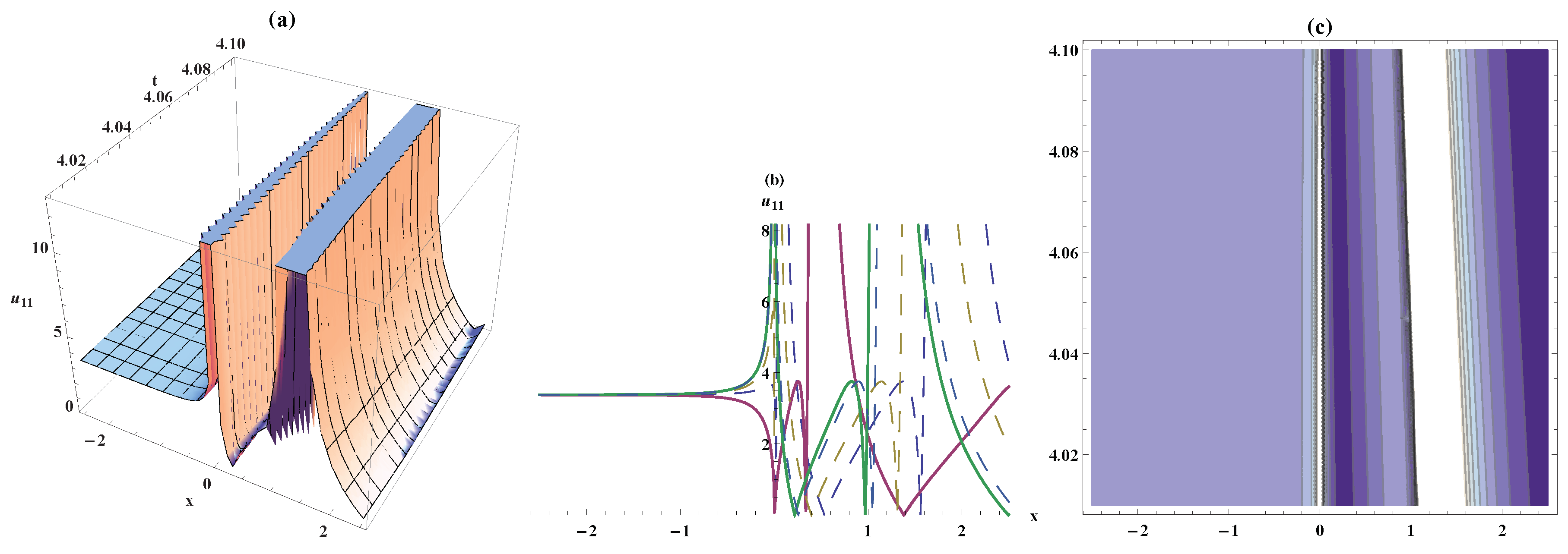
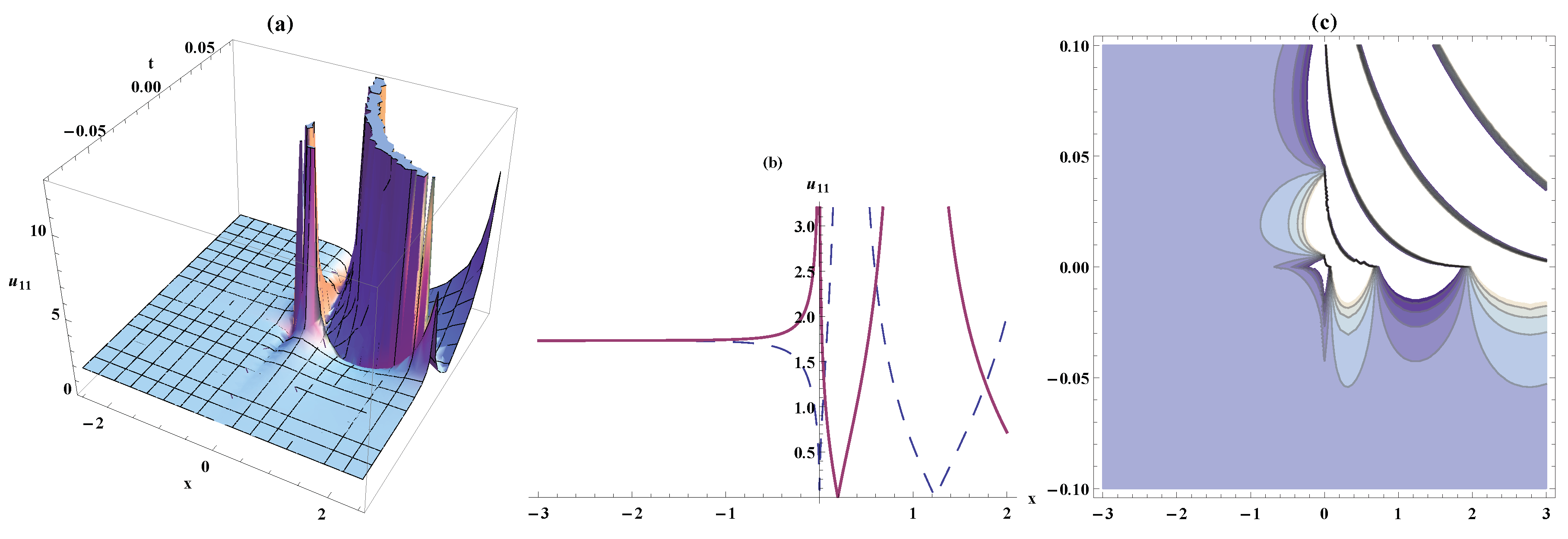
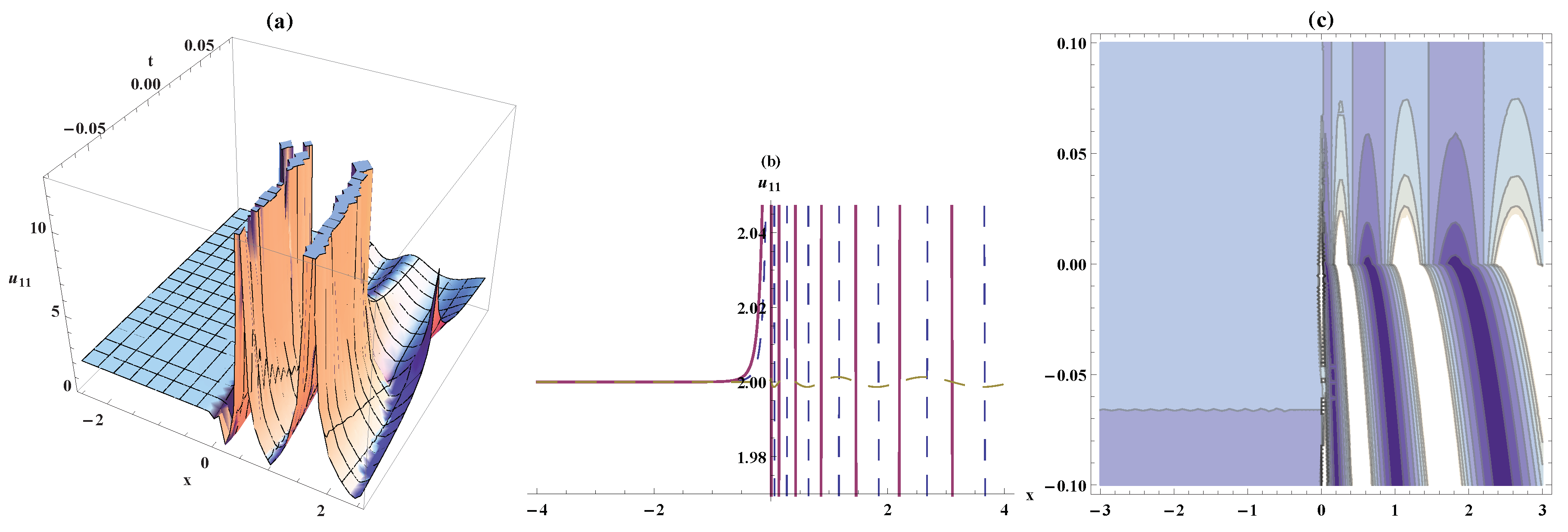
4. Results and Discussion

We examined a modified auxiliary equation method on three fundamental models in biological science. We discussed two approaches to the comparison of our solutions and results in [43]. The first kind is a numerical comparison which depends on a number of solutions for each paper. We obtained many solutions for each model, but Guner and Bekir found just a few for each of these models. The second kind of comparison is the novelty of solutions. We obtained many solutions, covering all solutions obtained in [43] as well as other different solutions to those obtained in the mentioned paper. The novelty of this paper lies in the progress in these models. Guner and Bekir used a modified Riemann–Liouville derivative in imitation of changing the nonlinear fractional partial differential equations (NFPDEs) among an integer rule over normal differential equations (IOODEs). Many papers have confirmed the error in this kind of derivative.

5. Conclusions

In this paper, we applied well-established conformable derivative properties to three basic models in biological science. We also introduced a novel technique (modified auxiliary equation method or modified Khater method). We used this method on the converting ordinary equation of each model such that these models are fractional nonlinear partial differential equations. We obtained many novel solutions for each model. These solutions give more details and explanations of these models. We plotted solitary wave, bistable wave, and contour plots for some of our obtained solutions in Figure 1, Figure 2 and Figure 3 to give more explanations about these solutions. The accuracy of all obtained solutions was examined by putting them into their original equations using Mathematica 9.

References

1. Mei, F.X. Lie symmetries and conserved quantities of constrained mechanical systems. Acta Mech. 2000, 141, 135–148. [Google Scholar] [CrossRef]
2. Berezinskii, V.L. Destruction of long-range order in one-dimensional and two-dimensional systems having a continuous symmetry group I. Classical systems. Sov. Phys. JETP 1971, 32, 493–500. [Google Scholar]
3. Wegner, F. The mobility edge problem: Continuous symmetry and a conjecture. Z. Phys. B Condens. Matter 1979, 35, 207–210. [Google Scholar] [CrossRef]
4. Ibragimov, N.K.; Ibragimov, N.K. Elementary Lie Group Analysis and Ordinary Differential Equations; Wiley: New York, NY, USA, 1999. [Google Scholar]
5. Dorodnitsyn, V.A. Finite difference models entirely inheriting continuous symmetry of original differential equations. Int. J. Mod. Phys. C 1994, 5, 723–734. [Google Scholar] [CrossRef]
6. Kegeles, A.; Oriti, D. Continuous point symmetries in group field theories. J. Phys. A Math. Theor. 2017, 50, 125402. [Google Scholar] [CrossRef]
7. Lee, S.T.; Brockenbrough, J.R. A new approximate analytic solution for finite-conductivity vertical fractures. SPE Form. Eval. 1986, 1, 75–88. [Google Scholar] [CrossRef]
8. Comrey, A.L. Factor-analytic methods of scale development in personality and clinical psychology. J. Consult. Clin. Psychol. 1988, 56, 754. [Google Scholar] [CrossRef] [PubMed]
9. Chen, C.J.; Chen, H.C. Finite analytic numerical method for unsteady two-dimensional Navier-Stokes equations. J. Comput. Phys. 1984, 53, 209–226. [Google Scholar] [CrossRef]
10. Khater, M.M.A.; Lu, D.; Zahran, E.H.M. Solitary wave solutions of the Benjamin-Bona-Mahoney-Burgers equation with dual power-law nonlinearity. Appl. Math. Inf. Sci. 2017, 11, 1–5. [Google Scholar] [CrossRef]
11. Liao, S.J. On the analytic solution of magnetohydrodynamic flows of non-Newtonian fluids over a stretching sheet. J. Fluid Mech. 2003, 488, 189–212. [Google Scholar] [CrossRef]
12. Alart, P.; Curnier, A. A mixed formulation for frictional contact problems prone to Newton like solution methods. Comput. Methods Appl. Mech. Eng. 1991, 92, 353–375. [Google Scholar] [CrossRef]
13. Wertheim, M.S. Analytic solution of the Percus-Yevick equation. J. Math. Phys. 1964, 5, 643–651. [Google Scholar] [CrossRef]
14. Liao, S.J. A uniformly valid analytic solution of two-dimensional viscous flow over a semi-infinite flat plate. J. Fluid Mech. 1999, 385, 101–128. [Google Scholar] [CrossRef]
15. Liu, M.Z.; Li, D. Properties of analytic solution and numerical solution of multi-pantograph equation. Appl. Math. Comput. 2004, 155, 853–871. [Google Scholar] [CrossRef]
16. Khater, M.M.; Kumar, D. New exact solutions for the time fractional coupled Boussinesq-Burger equation and approximate long water wave equation in shallow water. J. Ocean Eng. Sci. 2017, 2, 223–228. [Google Scholar] [CrossRef]
17. Morales-Delgado, V.F.; Gómez-Aguilar, J.F.; Yépez-Martínez, H.; Baleanu, D.; Escobar-Jimenez, R.F.; Olivares-Peregrino, V.H. Laplace homotopy analysis method for solving linear partial differential equations using a fractional derivative with and without kernel singular. Adv. Differ. Equ. 2016, 2016, 164. [Google Scholar] [CrossRef]
18. Gómez-Aguilar, J.F.; Yépez-Martínez, H.; Torres-Jiménez, J.; Córdova-Fraga, T.; Escobar-Jiménez, R.F.; Olivares-Peregrino, V.H. Homotopy perturbation transform method for nonlinear differential equations involving to fractional operator with exponential kernel. Adv. Differ. Equ. 2017, 2017, 68. [Google Scholar] [CrossRef]
19. Yépez-Martínez, H.; Gómez-Aguilar, J.F.; Sosa, I.O.; Reyes, J.M.; Torres-Jiménez, J. The Feng’s first integral method applied to the nonlinear mKdV space-time fractional partial differential equation. Rev. Mex. Fís. 2016, 62, 310–316. [Google Scholar]
20. Gómez-Aguilar, J.F.; Atangana, A. New insight in fractional differentiation: power, exponential decay and Mittag-Leffler laws and applications. Eur. Phys. J. Plus 2017, 132, 13. [Google Scholar] [CrossRef]
21. Yépez-Martínez, H.; Gómez-Aguilar, J.F.; Atangana, A. First integral method for non-linear differential equations with conformable derivative. Math. Model. Nat. Phenom. 2018, 13, 14. [Google Scholar] [CrossRef]
22. Hammad, M.A.; Khalil, R. Abel’s formula and wronskian for conformable fractional differential equations. Int. J. Differ. Equ. Appl. 2014, 13. [Google Scholar] [CrossRef]
23. Khalil, R.; Al Horani, M.; Yousef, A.; Sababheh, M. A new definition of fractional derivative. J. Comput. Appl. Math. 2014, 264, 65–70. [Google Scholar] [CrossRef]
24. Abdeljawad, T. On conformable fractional calculus. J. Comput. Appl. Math. 2015, 279, 57–66. [Google Scholar] [CrossRef]
25. Chung, W.S. Fractional Newton mechanics with conformable fractional derivative. J. Comput. Appl. Math. 2015, 290, 150–158. [Google Scholar] [CrossRef]
26. Atangana, A.; Baleanu, D.; Alsaedi, A. New properties of conformable derivative. Open Math. 2015, 13, 889–898. [Google Scholar] [CrossRef]
27. Çenesiz, Y.; Baleanu, D.; Kurt, A.; Tasbozan, O. New exact solutions of Burgers’ type equations with conformable derivative. Waves Random Complex Media 2017, 27, 103–116. [Google Scholar] [CrossRef]
28. Hosseini, K.; Mayeli, P.; Ansari, R. Modified Kudryashov method for solving the conformable time-fractional Klein-Gordon equations with quadratic and cubic nonlinearities. Optik Int. J. Light Electron Opt. 2017, 130, 737–742. [Google Scholar] [CrossRef]
29. Hosseini, K.; Bekir, A.; Ansari, R. New exact solutions of the conformable time-fractional Cahn-Allen and Cahn-Hilliard equations using the modified Kudryashov method. Optik Int. J. Light Electron Opt. 2017, 132, 203–209. [Google Scholar] [CrossRef]
30. Latifizadeh, H. Application of homotopy analysis transform method to fractional biological population model. Rom. Rep. Phys. 2013, 65, 63–75. [Google Scholar]
31. Srivastava, V.K.; Kumar, S.; Awasthi, M.K.; Singh, B.K. Two-dimensional time fractional-order biological population model and its analytical solution. Egypt. J. Basic Appl. Sci. 2014, 1, 71–76. [Google Scholar] [CrossRef]
32. Baleanu, D.; Uǧurlu, Y.; Kilic, B. Improved (G/G)-Expansion Method for the Time-Fractional Biological Population Model and Cahn-Hilliard Equation. J. Comput. Nonlinear Dyn. 2015, 10, 051016. [Google Scholar] [CrossRef]
33. Singh, J.; Kumar, D.; Kılıçman, A. Numerical solutions of nonlinear fractional partial differential equations arising in spatial diffusion of biological populations. Abstr. Appl. Anal. 2014, 2014, 535793. [Google Scholar] [CrossRef]
34. Shakeri, F.; Dehghan, M. Numerical solution of a biological population model using He’s variational iteration method. Comput. Math. Appl. 2007, 54, 1197–1209. [Google Scholar] [CrossRef]
35. Morrison, P.J.; Meiss, J.D.; Cary, J.R. Scattering of regularized-long-wave solitary waves. Phys. D Nonlinear Phenom. 1984, 11, 324–336. [Google Scholar] [CrossRef]
36. Yusufoglu, E.; Bekir, A. Numerical simulation of equal-width wave equation. Comput. Math. Appl. 2007, 54, 1147–1153. [Google Scholar] [CrossRef]
37. Esen, A. A numerical solution of the equal width wave equation by a lumped Galerkin method. Appl. Math. Comput. 2005, 168, 270–282. [Google Scholar] [CrossRef]
38. Lu, D.; Seadawy, A.R.; Ali, A. Dispersive traveling wave solutions of the Equal-Width and Modified Equal-Width equations via mathematical methods and its applications. Results Phys. 2018, 9, 313–320. [Google Scholar] [CrossRef]
39. Korkmaz, A. Exact solutions of space-time fractional EW and modified EW equations. Chaos Solitons Fractals 2017, 96, 132–138. [Google Scholar] [CrossRef] [Green Version]
40. Wazwaz, A.M. The tanh and the sine-cosine methods for a reliable treatment of the modified equal width equation and its variants. Commun. Nonlinear Sci. Numer. Simul. 2006, 11, 148–160. [Google Scholar] [CrossRef]
41. Zaki, S.I. Solitary wave interactions for the modified equal width equation. Comput. Phys. Commun. 2000, 126, 219–231. [Google Scholar] [CrossRef]
42. Khalique, C.M.; Adem, K.R. Exact solutions of the (2+1)-dimensional Zakharov-Kuznetsov modified equal width equation using Lie group analysis. Math. Comput. Model. 2011, 54, 184–189. [Google Scholar] [CrossRef]
43. Guner, O.; Bekir, A. A novel method for nonlinear fractional differential equations using symbolic computation. Waves Random Complex Media 2017, 27, 163–170. [Google Scholar] [CrossRef]
Figure 1. (a) Solitary wave, (b) bistable wave amplitude, and (c) contour plots for Equation (13) in the respective interval { x , 2.05 , 2.05 } , { t , 0.08 , 0.08 } .
Mca 24 00001 g001
Figure 2. (a) Solitary wave, (b) the bistable wave amplitude and (c) contour plots for Equation (33) in the respective interval { x , 2.05 , 2.05 } , { t , 0.08 , 0.08 } .
Mca 24 00001 g002
Figure 3. (a) Solitary wave, (b) the bistable wave amplitude and (c) contour plots for Equation (53) in the respective interval { x , 2.05 , 2.05 } , { t , 0.08 , 0.08 } .
Mca 24 00001 g003