1. Introduction
Predictive numerical simulations in solid mechanics require material laws that involve systems of highly nonlinear Differential Algebraic Equations (DAEs). These models are essential in challenging industrial applications, for instance to study the effects of the extreme thermo-mechanical loadings that turbine blades may sustain in helicopter engines ([
1,
2]), as well as in biomechanical analyses [
3,
4].
These DAE systems are referred to as constitutive laws in the material science community. They express, for a specific material, the relationship between the mechanical quantities such as the strain, the stress, and miscellaneous internal variables and stand as the closure relations of the physical equations of mechanics. When the model aims to reproduce physically-complex behaviors, constitutive equations are often tuned through numerous parameters called material coefficients.
An appropriate calibration of these coefficients is necessary to ensure that the numerical model mimics the actual physical behavior [
5]. Numerical parametric studies, consisting of analyzing the influence of the parameter values on the solutions, are typically used to perform the identification. However, when the number of parameters increases and unless the computational effort required for a single numerical simulation is negligible, the exploration of the parameter domain turns into a tedious task, and exhaustive analyses become unfeasible. Moreover, defining an unambiguous criterion measuring the fidelity of the model to experimental data is a challenge for models with complex behaviors.
A common technique to mitigate the aforementioned challenges is to build surrogate models (or metamodels) mapping points of a given parameter space (considered as the inputs of the model) to the outputs of interest of the model. The real-time prediction of DAE solutions for arbitrary parameter values, enabled by the surrogate model, helps the comprehension of constitutive laws and facilitates the conducting of parametric studies. In particular, the robustness of the calibration process can be dramatically improved using surrogate model approaches.
The idea of representing the set of all possible parameter-dependent solutions of ODEs and PDEs as a multiway tensor was pioneered with the introduction of the Proper Generalized Decomposition (PGD) [
6,
7,
8]. In this representation, each dimension corresponds to a spatial/temporal coordinate or a parameter coefficient. The resulting tensor is never assembled explicitly, but instead remains an abstract object for which a low-rank approximation based on a canonical polyadic decomposition [
9] is computed. The PGD method further alleviates the curse of dimensionality by introducing a multidimensional weak formulation over the entire parameter space, and the solutions are sought in a particular form where all variables are separated. When differential operators admit a tensor decomposition, the PGD method is very efficient because the multiple integrals involved in the multidimensional weak form of the equations can be rewritten as a sum of products of simple integrals.
Unfortunately, realistic constitutive equations or even less sophisticated elasto-viscoplastic models admit no tensor decomposition with respect to the material coefficients and the time variables. An extension of the PGD to highly nonlinear laws is therefore non-trivial. However, many other tensor decomposition approaches have been successfully proposed to approximate functions or solutions of differential equations defined over high-dimensional spaces. We refer the reader to [
10,
11,
12] for detailed reviews on tensor decomposition techniques and their applications.
Among the existing formats—CP decomposition [
9,
13,
14], Tucker decomposition [
11,
15], hierarchical Tucker decomposition [
11,
16]—this work investigates the Tensor-Train (TT) decomposition [
17,
18]. The TT-cross algorithm, introduced in [
17] and further developed in [
19,
20], is a sampling procedure to build an approximation of a given tensor under the tensor-train format. Sampling procedures in parameter space have proven their ability to reduce nonlinear and non-separable DAEs by using the Proper Orthogonal Decomposition (POD) [
21], the gappy POD [
22], or the Empirical Interpolation Method (EIM) [
23,
24]. These last methods are very convenient when the solutions have only two variables; hence, they are considered as second-order tensors.
This paper aims to extend the sampling procedure of the TT-cross method to DAEs having heterogeneous and time-dependent outputs. A common sampling of the parameter space is proposed, though several TT-cross approximations are computed to cope with heterogeneous outputs. These outputs can be scalars, vectors, or tensors, with various physical units. In the proposed algorithm, sampling points are not specific to any output, although parameters do not affect equally each DAE output. The proposed method is named multiple TT-cross approximation. Similarly to the construction of a reduced integration domain for the hyper-reduction of partial differential equations [
25] or for the GNATmethod [
26], the set of sampling points is the union of contributions from the various outputs of the DEA. In this paper, the multiple TT-cross incorporates the gappy POD method, and the developments are focused on the numerical outputs obtained through a numerical integration scheme applied to the DAE.
2. Materials and Methods
The parametrized material model generates several time-dependent Quantities of Interest (QoI). These quantities can be scalar-, vector-, or even tensor-valued (e.g., stress) and are generally of distinct natures, namely expressed with different physical units and/or have different magnitudes. For instance, in the physical model described in
Appendix A, the outputs of the model are
,
,
, and
, where
t is the time variable,
,
,
have six components each, and
p is a scalar. Therefore, the generated data will be segregated according to the QoI to which they relate. This will also be structured in a tensor-like fashion to make it amenable to the numerical methods presented in this paper. We restrict our attention to discrete values of
parameters and discrete values of time instants, related to indices
,
for
. For instance, all the computable scalar outputs
p will be considered as a tensor
.
For a given
denoting an arbitrary QoI, the tensor of order
d,
(denoted with bold calligraphic letters) refers to a multidimensional array (also called a multiway array). Each element of
identified by the indices
is denoted by:
where
for
is the set of natural numbers from one to
(inclusive) and
. The last index accounts for the number of components in each QoI. Therefore, the last index is specific to each
, while the others are common to all tensors for
. Hence, a common sampling of the parameter space
can be achieved. The vector
contains all the components of output
at all time instants used for the numerical solution of the DAE and for a given point in the parameter space.
Matricization designates a special case of tensor reshaping that allows representing an arbitrary tensor as a matrix. The
matricization of
denoted by
consists of dividing the dimensions of
into two groups, the
q leading dimensions and the
trailing dimensions, such that the newly-defined multi-indices enumerate respectively the rows and columns of the matrix
. For instance,
and
are matrices of respective sizes
-by-
and
-by-
. Their elements are given by:
where
enumerates the multi-index
and
enumerates the multi-index
. Here again, these matricizations are purely formal because of the curse of dimensionality.
The Frobenius norm is denoted by ||.||. without the usual subscript
. For
, it reads:
The Frobenius norm of a tensor is invariant under all matricizations of a given tensor.
In [
17], Singular-Value Decomposition (SVD) is considered in the algorithm called TT-SVD. Because of the curse of dimensionality, the TT-SVD has no practical use, even if tensors have a low rank. More workable approaches aim to sample the entries of tensors.
For instance, in the snapshot Proper Orthogonal Decomposition (POD) [
21], the sampling procedure aims to estimate the rank and an orthogonal reduced basis for the approximation of a matrix
A. The method consists of applying the truncated SVD on the submatrix
constituted by a selection of columns
of
A. Hence, the accuracy of the resulting POD reduced basis relies on the quality of the sampling procedure that generally introduces a sampling error. This sampling procedure seems to be convenient when considering the first matricizations
if the product
and
are reasonably small regarding the available computing resources. However,, for large values of
q, the curse of dimensionality makes the snapshot POD, alone, intractable.
A more practical approach to construct an approximate TT decomposition effectively, called the TT-cross method, is proposed in [
17]. The TT-cross consists of dropping the concept of a POD basis and using the Pseudo-Skeleton Decomposition (PSD) introduced in [
27] as the low-rank approximation. Unlike the TT-SVD, the TT-cross enables building an approximation based on a sparse exploration of a reference tensor. The PSD can be used to approximate any matrix
and is written as:
where the sets
and
are respectively a selection of row and column indices. The definition is valid only when the matrix
is non-singular. In particular, the number
s of rows and columns has to be identical.
This approximation (
1) features an interpolation property at the selected rows and columns:
The PSD is a matrix factorization similar to the decomposition used in the Adaptive Cross Approximation (ACA) [
28] and the CURdecomposition [
29,
30]. Additionally, these references provide algorithms to build the factorization effectively. That decomposition has also been used in the context of model order reduction, for instance in the Empirical Interpolation Method (EIM) proposed in [
23,
24].
The condition that must be non-singular makes it difficult to share sampling points for various matrices with having their own rank.
The gappy POD introduced in [
22] aims at relaxing the aforementioned constraint by combining beneficial features of the snapshot POD and the PSD. Indeed, the gappy POD (a) relies on a POD basis that remains computationally affordable, (b) requires only a limited number of rows of the matrix to be approximated, and (c) enables reusing the set of selected rows for different matrices. These properties are key ingredients for an efficient, parsimonious exploration of the reference tensors. The gappy POD approximation
of a matrix
is given by:
where † denotes the Moore–Penrose pseudo-inverse [
31] and
is a row selection of
s rows and where
is a POD basis matrix of rank
r such that:
In the sequel, because the simulation data in
are outputs of a DAE system, it does not make sense to sample the last index
during column sampling of
. Each numerical solution of the DAE system generates all the last components of each tensor
. Hence, the column sampling is restricted to indices
, and all the values of
in
are kept. This special column sampling is denoted by
. It is performed randomly by using a low-discrepancy Halton sequence [
32].
The matrix
must have linearly independent columns to ensure that the approximation is meaningful. Since is a rank-
r POD basis, there exists a set of
s rows such that this property holds as long as
. Here,
contains at least the interpolation indices related to
V. This latter set is denoted by
, such that
is invertible. In the numerical results presented hereafter,
is obtained using the Q-DEIM algorithm [
33] that was shown to be a superior alternative to the better-known DEIM procedure ([
34], Algorithm 1).
Unlike the PSD, the gappy POD enables selecting a number of rows that exceeds the rank of the low-rank approximation:
This makes it possible to share sampling points between matrices having their own rank. In this case, the interpolation property does not hold as in the PSD case (
2).
is the approximation of by the product of three matrices:
V,
and
. The TT-cross approximation can be understood as a generalization of such a product of matrices. A tensor
is said to be in Tensor-Train format (TT format) if its elements are given by the following matrix products:
where the so-called tensor carriages (or core tensors) are such that for
:
In the original definition of the tensor-train format [
17], the leading and trailing factors (corresponding to
and
for any choice of
and
) are respectively row and column vectors. Here, the convention
is adopted so that row matrices
and column matrices
can be interpreted as vectors or matrices depending on the context.
The TT format allows significant gains in terms of memory storage and therefore is well-suited to high-order tensors. The storage complexity is
where
and depends linearly on the order
d of the tensor. In many applications of practical interest, the small TT-ranks
enable alleviating the curse of dimensionality [
17].
The sequential computational complexity of the evaluation of a single element of a tensor in TT format is
. Assuming that
is small enough, the low computational cost allows a real-time evaluation of the underlying tensor. Therefore, in terms of online exploitation, this representation conforms with the expected requirements of the surrogate model.
Figure 1 illustrates the sequence of matrix multiplications required to compute one element of the tensor train.
The objective of the proposed approach is to build for each physics-based tensor an approximate tensor given in TT format by using a nested row sampling of the simulation data. Algorithm 1 provides the set of matrices that enable defining the tensor-train decompositions and aggregate sets for row sampling. It is a sequential algorithm that navigates from dimension one to dimension of tensors .
The method provided by Algorithm 1 is non-intrusive and relies on the numerical solutions of the DAEs in a black-box fashion.
| Algorithm 1: Multiple TT Decomposition. |
![Mca 24 00017 i001]() |
At each iteration
, the snapshot POD method, used to build the POD reduced basis (9), requires sampling a set
. The column sampling amounts to a parsimonious selection of
points in the partial discretized parameter domain
and an exhaustive sampling of the last dimension for each tensor
. The considered submatrices
are then constituted of
columns (see
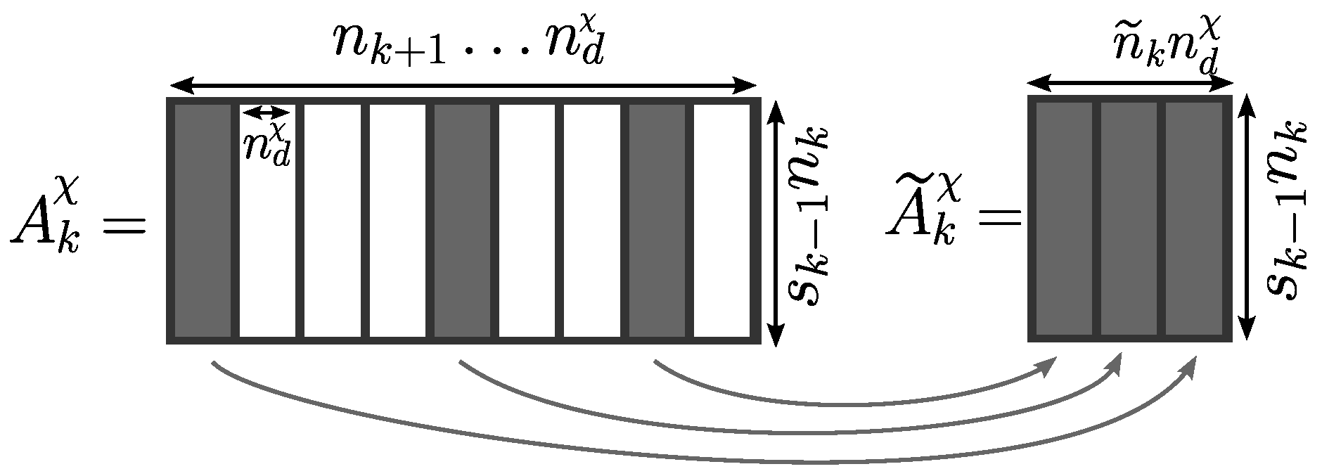
Figure 2).
In the row sampling step, specific sets of interpolant rows are first determined independently for each output , but a common, aggregated set (10) is then used to sample the entries of all outputs. Indeed, computing the elements of all submatrices requires calls to the DAE system solver with: with . Furthermore, the gappy POD naturally accommodates a number of rows larger than the rank for each approximation of , and considering a larger sample size for each individual is expected to provide a more accurate approximation.
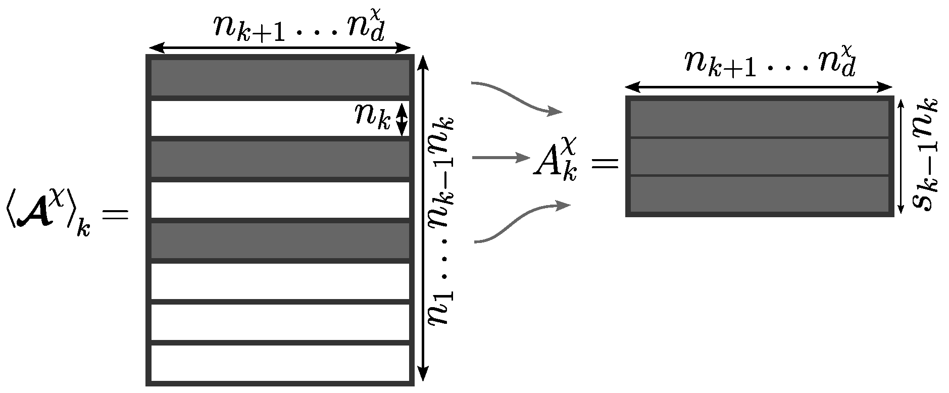
The tensorization and matricization steps are purely formal. No call to the DAE system solver is done here. They define the way the simulation data must be ordered in matrices to be approximated at the next iteration. The recursive definition of the matrix
implies that the latter is equal to the
kth matricization of a subtensor extracted from
. Equivalently, the matrix
corresponds to a submatrix of the
kth matricization of
, as illustrated in
Figure 3.
To quantify the theoretical accumulation of errors introduced at each iteration, Proposition 1 gives an upper bound for the approximation error associated with a tensor-train decomposition built by the snapshot POD followed by the row sampling steps, when a full column sampling is performed.
Proposition 1. Consider and its tensor-train approximation constructed by Algorithm 1. Assuming that for all :the following inequality holds:where and refer to the smallest and the largest singular values of its matrix argument. The proof is given in ([
35], Proposition 12).
Proposition 1 suggests that the approximation error
can be controlled by the truncation tolerances
set by the user. However, the bound (
16) tends to be very loose, and the hypothesis (
15) may be difficult to verify when the basis
stems from a column sampling of the matrix
. Hence, the convergence should be assessed empirically in practical cases.
3. Results
3.1. Outputs’ Partitioning as Formal Tensors
The physical model described in
Appendix A is represented as the relations between six (
) parameters (inputs of the model) and the time-dependent mechanical variables (outputs of the model):
where
,
,
have six components each and pis a scalar.
,
, and
p have the same units, but have different physical meanings.
The surrogate model is defined by introducing groups of outputs as tensors . The formal tensors , … are related to p, , , and , respectively.
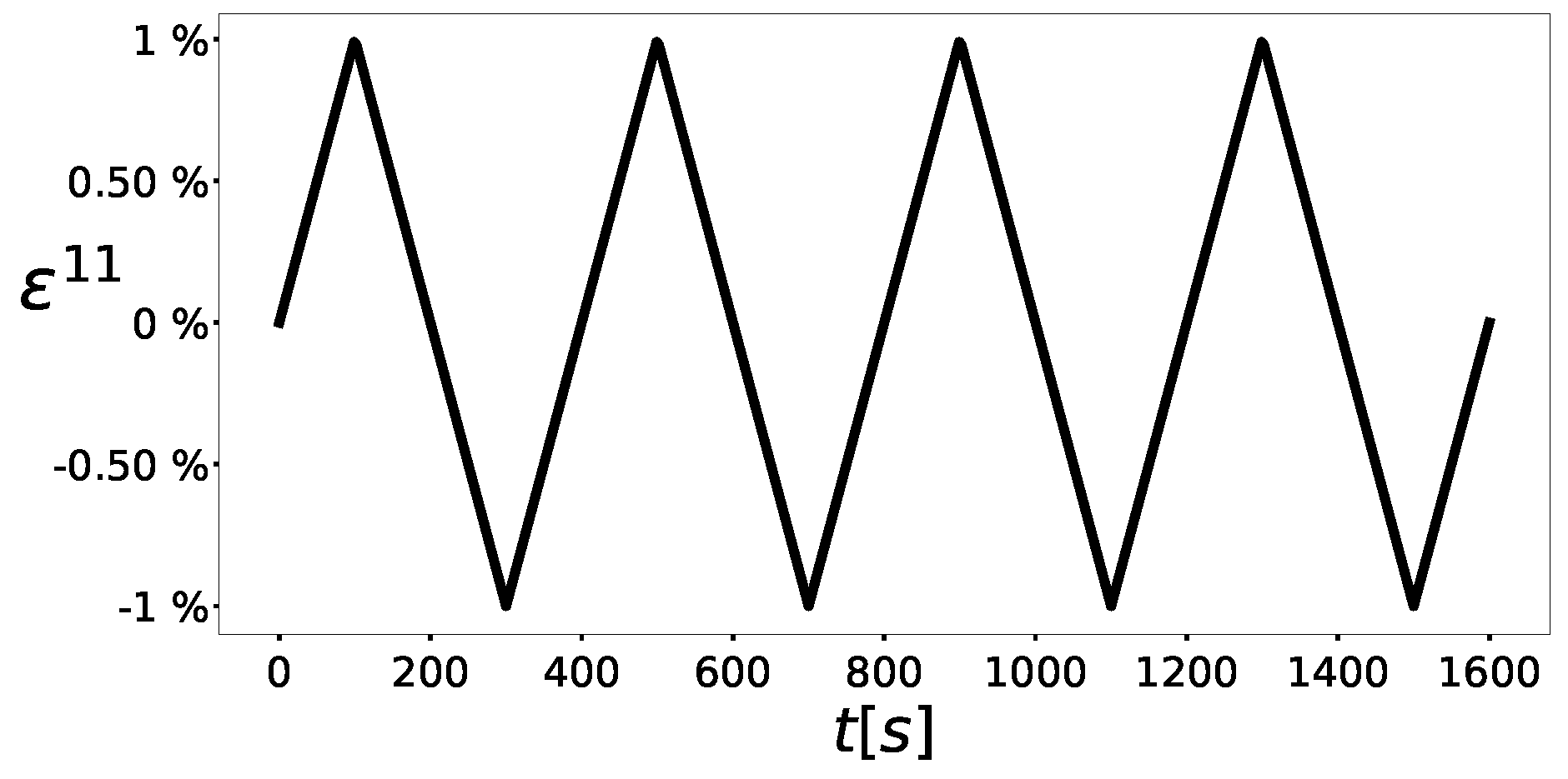
For each parameter, the interval of definition is discretized by a regular grid with 30 points:
The time interval discretized is the one used for the numerical solution; it corresponds to a regular grid with
points. Then:
The snapshot POD sample sizes are:
3.2. Performance Indicators
The truncation tolerance is chosen here to be . The construction of the tensor-train decompositions requires solving the system of DAEs times with as many sets of parameter values. In the proposed numerical example, it amounts to solutions. Fifteen hours were necessary on a 16-core workstation to carry out the computations. Ninety eight percent of the effort was devoted to the solution of the physical model and the remaining to the decomposition operations.
For a single simulation on a personal laptop computer, the solution of the physical model took s, whereas the surrogate model was evaluated in only 1 ms, corresponding to a speed-up of 700.
Storing the multiple TT approximations requires 2,709,405 double-precision floating-point values. For comparison purposes, storing a single solution (constituted by the multiple time-dependent outputs) of the DAE system involves 10,203 values. Therefore, the storage of the tensor-train decompositions is commensurate with the storage of 265 solutions, while it can express the approximation of solutions.
For
, the rank
is bounded from above by the theoretical maximum rank
of the matrix
. More specifically,
corresponds to the case where
has full rank and is the
kth matricizations of the tensors
. Given the choice of truncation tolerance
, the TT-ranks listed in
Table 1 show that the resulting tensor trains involve low rank approximations.
Table 2 emphasizes that in practice,
except for
where
is already “small”.
3.3. Approximation Error
The accuracy of the surrogate model is estimated a posteriori by measuring the discrepancy between its own outputs and the outputs of the original physical model. The estimation is conducted by comparing solutions associated with 20,000 new samples of parameter set values randomly selected according to a uniform law on each discretized parameter interval. The difference between the surrogate and the physical models is measured based on the following norms:
where
x and
are respectively scalar and tensor time-dependent functions.
For the mechanical variable Z (where Z can stand for any one of , , and p), and denote the output corresponding respectively to the solution of the DAEs and the surrogate model. A relative error is associated with each mechanical variable, namely:
Total Strain Tensor: ;
Viscoplastic Strain Tensor: ;
Stress Tensor: ;
Cumulative Viscoplastic Deformation: .
Depending on the parameter values, the viscoplastic part of the behavior may or may not be negligible as measured by the magnitudes of ||p|| and relative to . Hence, in the proposed application, the focus is on comparing the norm of the approximation error for , , and p with respect to the norm of .
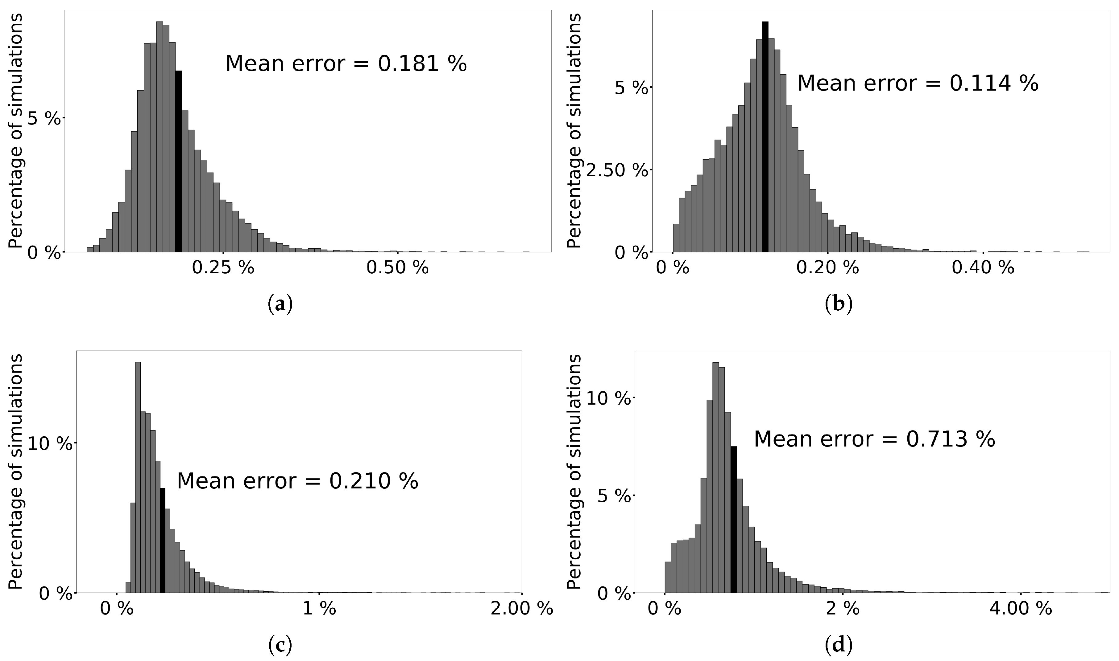
The histograms featured in
Figure 4a–d present, for each mechanical variables, the empirical distribution of the relative error for all simulation results. The surrogate model given by the tensor-train decompositions features a level of error that is sufficiently low to carry out parametric studies such as the calibration of constitutive laws where errors lower than
are typically tolerable.
3.4. Convergence with Respect to the Truncation Tolerance
A first surrogate model is constructed from the physical model with the prescribed truncation tolerance
. Then, this first surrogate model is used as an input for Algorithm 1. Running the algorithm several times with different truncation tolerances:
generates as many new surrogate models.
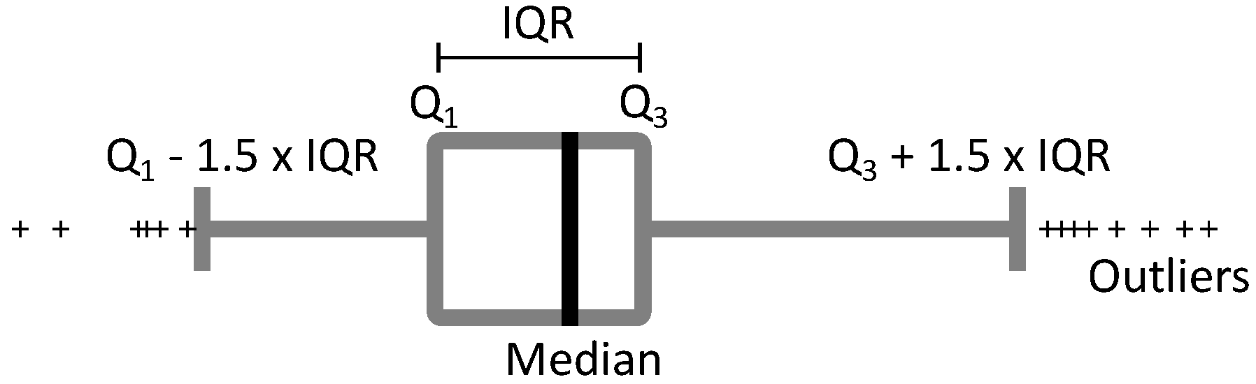
Figure 5a–d present the evolution of the relative error distribution (for the different mechanical variables) with respect to the truncation tolerance based on a random sample of 20,000 parameter set values chosen as in
Section 3.3.
Figure 6 details the graphical notations. The results empirically show for each mechanical output that the relative error decreases together with
. This is consistent with the expected behavior of the algorithm.
The plots in
Figure 7a,b show the dependence of the number of stored elements and the number of calls to the physical model on
.
3.5. On Fly Error Estimation
Based on the physical model, the surrogate model gives an approximation of each output of interest. However, the approximate outputs may be inconsistent with the physics in the sense that they may lead to non-zero residuals when introduced into (the discrete version of) the DAE system describing the physical model.
A coherence estimator is an indicator that measures how closely the physical equations are verified by the outputs of the surrogate model. It is reasonable to expect the accuracy of the metamodel to be correlated with the coherence estimator.
Using Equation (
A1), let:
and define the associated coherence estimator as follows:
and the effectivity of the estimator as the following ratio:
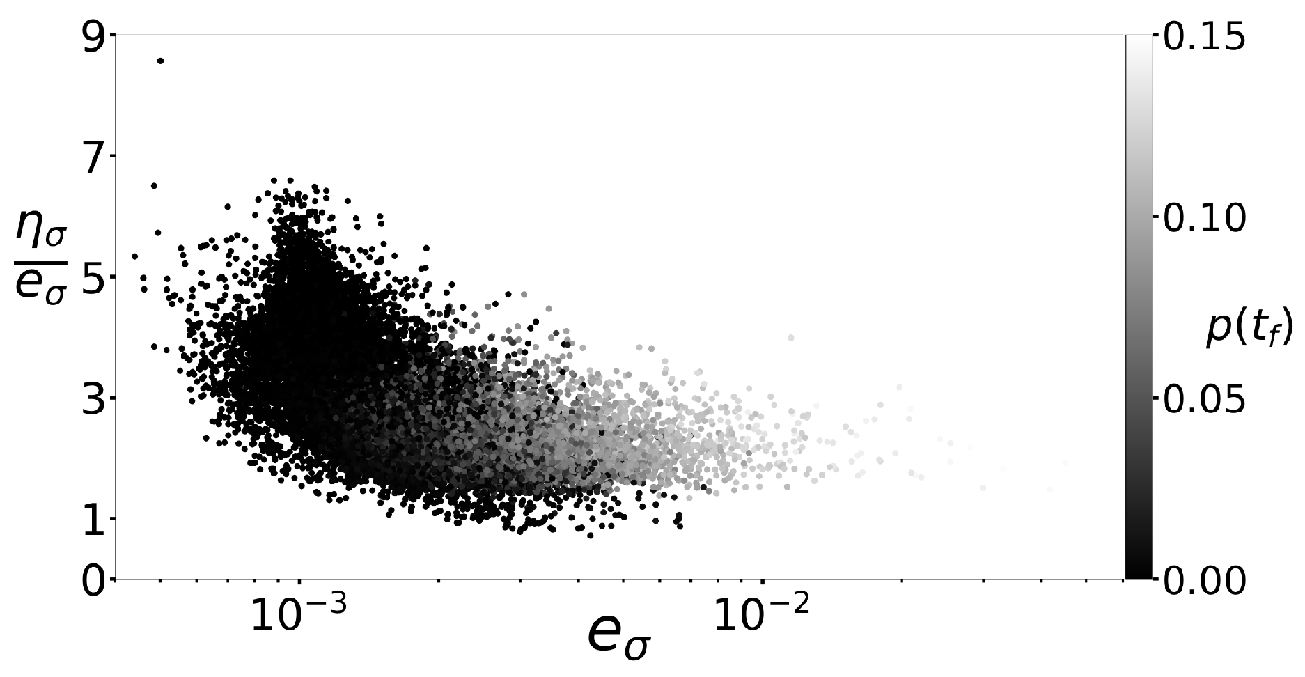
Figure 8 displays the relation between the relative error for and the effectivity of the estimator for 20,000 simulation results drawn randomly. The error increases with the final cumulative deformation, that is when the material exhibits a more intense viscoplastic behavior.
Furthermore, the plot shows a correlation between the coherence estimator and the relative error. In particular, the effectivity tends to be larger than one, which indicates that the coherence estimator behaves like an upper bound of the relative error. Excluding a few outliers, the coherence estimator does not overestimate the relative error by more than a factor of seven.
Finally, the effectivity of the coherence estimator empirically converges to one (that is, the estimator becomes sharper) as the magnitude of the relative error increases.
This coherence estimator is very inexpensive to compute and only relies on the outputs of the surrogate model. The results suggest that the coherence estimator could be used as an online error indicator that increases the reliability of the surrogate model at the current point when exploring in real time the parameter domain.


