Toward Optimality of Proper Generalised Decomposition Bases

Abstract

The solution of structural problems with nonlinear material behaviour in a model order reduction framework is investigated in this paper. In such a framework, greedy algorithms or adaptive strategies are interesting as they adjust the reduced order basis (ROB) to the problem of interest. However, these greedy strategies may lead to an excessive increase in the size of the ROB, i.e., the solution is no more represented in its optimal low-dimensional expansion. Here, an optimised strategy is proposed to maintain, at each step of the greedy algorithm, the lowest dimension of a Proper Generalized Decomposition (PGD) basis using a randomised Singular Value Decomposition (SVD) algorithm. Comparing to conventional approaches such as Gram–Schmidt orthonormalisation or deterministic SVD, it is shown to be very efficient both in terms of numerical cost and optimality of the ROB. Examples with different mesh densities are investigated to demonstrate the numerical efficiency of the presented method.

1. Introduction

Numerical simulations appeal as an attractive augmentation to experiments to design and analyse mechanical structures. Despite the recent developments in computational resources that makes it feasible to solve systems with a substantial number of degrees of freedom efficiently, it is of common interest to reduce the numerical cost of numerical models throughout model order reduction (MOR) strategies [1]. The performance of MOR techniques has been shown in different fields such as their application to nonlinear problems [2,3], real-time computations [4] or for performing cyclic, parametric or probabilistic computations in which the information provided by some queries can be efficiently reused to respond to other queries that exhibit some similarities [5,6].

A posteriori model reduction techniques such as the Proper Orthogonal Decomposition (POD) is based on an offline training computations which extract a reduced order basis (ROB) from the solution of a high fidelity model. This optimal basis is practically built through a singular value decomposition (SVD) of a snapshot matrix. The singular vectors corresponding to the highest singular values are used to build the ROB [7]. Then, the problem of interest is confined to this ROB resulting in a drastic reduction in the numerical cost [1,8]. However, since the ROB has been defined as an optimal basis for the training stage, some advanced adaptive approaches are required to enrich the basis to tackle nonlinearities [9]. On the other hand, a priori MOR technique such as the Proper Generalized Decomposition (PGD) is based on the assumption that the quantities of interest can be written as a finite sum of products of separated functions, of generalised coordinates, which are sought in online computations [8,10]. No prior knowledge of the system is required in such a case and the ROB is directly adapted to the problem of interest by using a greedy algorithm, which enriches the basis when required [3,11]. However, an issue may be caused by the rapid growth of the ROB basis, whereas the primary interest of MOR is to benefit from a small sized ROB which provides a nondemanding temporal updating step. This step is equivalent to a POD step where the spatial modes are fixed and only the temporal ones are updated. It has been observed that the basis can increase to count some hundreds of modes for parametric studies of nonlinear cyclic loading [12], or some thousands for parametric computations [13]. In [5], some advanced strategies have been proposed to use an optimal parametric path allowing for controlling the basis expansion optimally.

In the context of reusing an ROB from a previous computation, a learning strategy has been proposed in [14,15] to extract an optimal basis from the reduced order model (ROM) through a Karhunen–Loève expansion. In a PGD framework, recompression based on SVD has been evaluated in [16]. However, the SVD step turns out to be numerically expensive prohibiting its implementation at each iteration. Therefore, it is common to let the basis increase and compress the results only at convergence to decrease their storage requirements. Therefore, it appears of interest to investigate probabilistic algorithms to compress the ROB on-the-fly without creating a bottleneck in the ROM. A detailed review of the most established algorithms to compute an SVD is provided in [17,18]. These algorithms are not limited to conventional deterministic methods such as truncated, incremental or iterative SVD but also randomised algorithms [19]. Different algorithms have been tested for POD applications in the case of dynamical problems in [18]. It has been noticed that randomised SVD algorithms can reduce drastically the numerical cost of the decomposition required after the training stage. Even if this step occurs only once in the offline stage of POD based ROM, the number of degrees of freedom and time steps can be vast for the high fidelity model so that the decomposition process can be a bottleneck.

Our goal here is to maintain the flexibility of the greedy algorithm through the usage of PGD while controlling the size of the ROB with a minimal numerical cost, by proposing to use a randomised SVD algorithm that provides a nondemanding compressive step after each enrichment of the basis. The numerical approach will be herein exemplified for the specific case of a fatigue computation based on continuum damage mechanics in a large time increment (LATIN) framework. However, the proposed numerical strategy can be generally used to optimise efficiently PGD basis for any application.

This paper is structured as follows. An overview of the LATIN-PGD scheme is provided in Section 2, followed by a discussion on the optimality of the PGD modes and the different algorithms to ensure that in Section 3. Lastly, in Section 4, different numerical examples are presented to illustrate the robustness and efficiency of the proposed algorithm.

Notation

The notation used in this paper is summarised in

Table 1. Symbols and their representation.

Symbolic Representation	Verbal Representation
$a,\phi$	scalars: lowercase letters
$\mathit{u},\mathit{x}$	first-order tensors: lowercase boldface letters
$\mathit{I},\mathit{N}$	second-order tensors: uppercase boldface letters
$\mathit{\sigma },\mathit{\epsilon }$	second-order tensors: Greek boldface letters
$\mathbb{C},\mathbb{H}$	fourth-order tensor: blackboard bold letters
$\underline{a}$	column vector
$\underline{\underline{A}}$	matrix

.

2. An Overview of the LATIN-PGD Method

LATIN is a linearisation scheme that makes it easier to introduce PGD in nonlinear mechanical computations. A review of the LATIN-PGD method and some of its recent extensions to nonlinear solid mechanics problems can be found in [8,11].

The LATIN method is a fully discrete non-incremental solution scheme that inherits its efficiency for mechanical problems from incorporating an a priori model order reduction technique, namely PGD. It is shown in [20] that functions defined over space-time domain, with some regularities, may be approximated by PGD. However, it is vital that the number of modes (approximating functions) is small and the approximation error is low. A summary of the implemented framework is provided below.

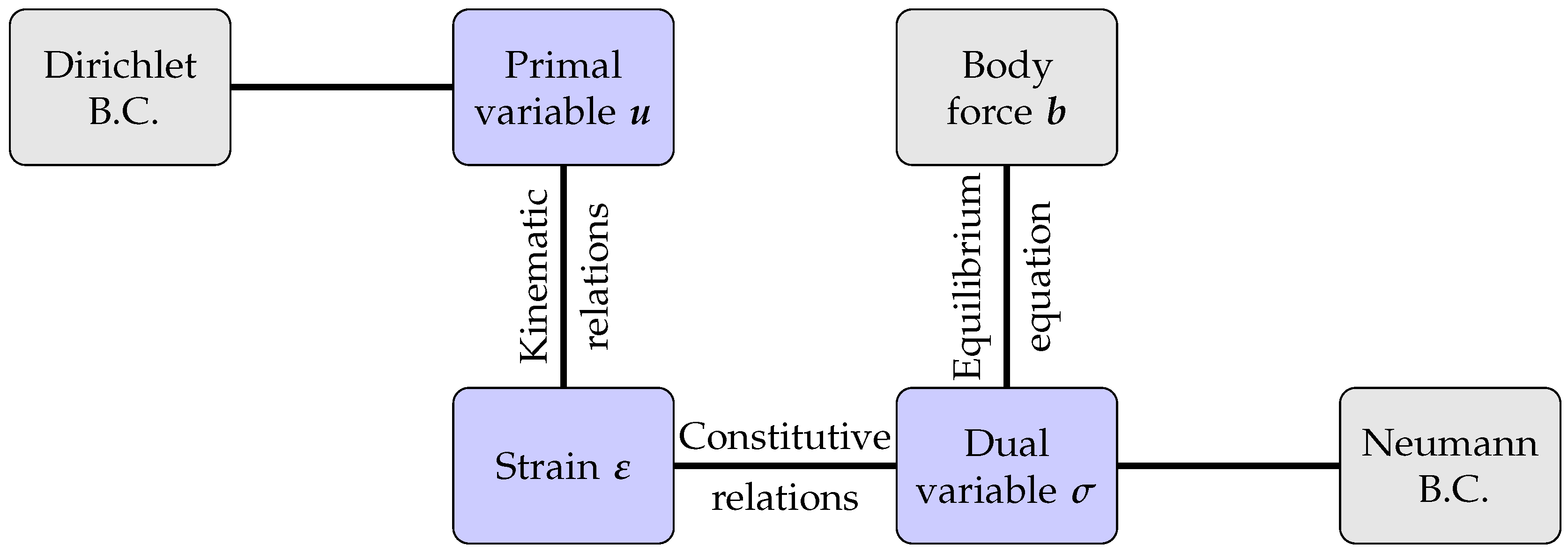
For a generic structural problem defined over space-time domain $\mathsf{\Xi }=\mathsf{\Omega }\times \mathcal{I}=\mathsf{\Omega }\times [0,T]$ in an infinitesimal strain and quasi-static framework, the strong form to be solved is represented in Figure 1 [21,22]. The equilibrium equation is linear in terms of the stress and the nonlinearity, in this case, is introduced through the constitutive model, i.e., in the stress–strain ($\mathit{\sigma },\mathit{\epsilon }$) relationship.

In a standard incremental Newton–Raphson scheme, the constitutive relations along with the kinematic relations are substituted into the balance equation resulting in a nonlinear problem in terms of the primal variable. However, a different linearisation strategy, termed LATIN, consists of solving the equilibrium equations along with kinematic relations in one step and solving the constitutive relations in the following step. Then, a solution that satisfies both of these systems is sought. In such a framework, two sets of equations are distinguished, the local equations described by constitutive relations (evolution and state laws [23]) and the global equilibrium equation along with the kinematic compatibility. Data flow between these two systems is required, i.e., to get statically admissible stress and kinematically permissible strain or displacement, a relation between the stress and the strain should be assumed. In the same manner, a decision should be taken on what data to pass back from the global system to the local one; these relations are referred to as search direction equations because they are affine equations in a 12-dimensional space hosting the stress and strain fields. The main advantage of the LATIN linearisation scheme is confining the computational cost to the solution of a global linear equation, which allows for introducing a model order reduction technique such as the PGD to reduce this numerical cost [8].

PGD is often used in many query context and quick response simulations where the solution is approximated by a finite sum of separated functions on each of the problem generalised coordinates, e.g., the displacement field may be approximated by a finite sum of globally spatial and temporal functions as

$${\displaystyle \mathit{u}(\mathit{x},t)\approx \sum _{j=1}^N{\mathit{v}}_j(\mathit{x})⚬{\mathit{\lambda }}_j(t),{\mathit{v}}_j(\mathit{x}):\mathsf{\Omega }\to {\mathbb{R}}^d,{\mathit{\lambda }}_j(t):\mathcal{I}\to \mathbb{R},}$$

(1)

where $d\le 3$ is the spatial dimension, $N\in \mathbb{N}$ and ⚬ is the entry-wise Hadamard or Schur multiplication of vectors [8,24]. It is shown in [8] that a small number of pairs/modes is sufficient to approximate the solution of many problems with substantial savings in terms of CPU time and memory. In contrary to POD based techniques that include a preliminary learning phase, PGD defines the basis of the problem on-the-fly using a greedy algorithm such that additional pairs are added if necessary, i.e., the approximation error is controlled by the successive enrichment of the generated basis [25].

The LATIN solution algorithm starts with an elastic initialisation followed by a sequence of two stages, namely the local and the global ones. These two steps form one LATIN iteration, and they are repeated until convergence is reached. Note that, at every local and global step, the quantities of interest over all the space-time points are approximated. The space that belongs to the solution manifold of the constitutive relations is denoted by $\mathsf{\Gamma }$ while $\mathcal{A}$ represents the admissible space that satisfies the equilibrium equation (static admissibility) along with the kinematic relations (kinematic admissibility). Hence, the exact solution is defined as a set $s=\{\mathit{X},\dot{\mathit{Y}}\}\in \mathsf{\Gamma }\cap \mathcal{A}$, where X contains the dynamic conjugate variables and $\dot{\mathit{Y}}$ represents the evolution of the internal variables. For discussions on the LATIN convergence behaviour, refer to [8,20,26].

The elastic solution $s_0=\{{\mathit{X}}_0\}$ takes all the boundary conditions into account, and the following solutions are computed in terms of corrections to $s_0$. Then, the constitutive model, consisting of the nonlinear evolution equations in addition to the state equations, is solved and integrated within the local stage at every space-time point. The outcome of this stage, at the $i^{\mathrm{th}}$ iteration, is the solution ${\widehat{s}}_i^{}=\{{\widehat{\mathit{X}}}_i^{},{\widehat{\dot{\mathit{Y}}}}_i^{}\},$ which is used in the following global stage to obtain $s_{i+1}^{}$. The admissibility equations are the only ones left to be solved in the global stage. The kinematic admissibility is satisfied by deriving the strain as the symmetric gradient of the displacement field $\mathit{\epsilon }={\nabla }^{\mathrm{s}}u$ with $u=\overline{u}$ on $\partial {\mathsf{\Omega }}_D$ and the static admissibility condition is obtained from the equilibrium equation, which reads [27]

$$\nabla ·\mathit{\sigma }(x,t)+b=0\forall (x,t)\in \mathsf{\Omega }\times \mathcal{I},$$

(2)

with $\mathit{\sigma }·n=\overline{t}$ on $\partial {\mathsf{\Omega }}_N$, $\mathit{\sigma }$ is Cauchy stress and b is the body force in the spatial domain $\mathsf{\Omega }$. The use of the Hamilton’s law of varying action, which is the principle of virtual work integrated over time [28], leads to the following weak form

$$\underset{\mathsf{\Omega }\times \mathcal{I}}{\int }\mathit{\sigma }:\mathit{\epsilon }({\mathit{u}}^{\ast })\mathrm{d}\mathsf{\Omega }\mathrm{d}t=\underset{\mathsf{\Omega }\times \mathcal{I}}{\int }\mathit{b}·{\mathit{u}}^{\ast }\mathrm{d}\mathsf{\Omega }\mathrm{d}t+\underset{\partial {\mathsf{\Omega }}_N\times \mathcal{I}}{\int }\overline{\mathit{t}}·{\mathit{u}}^{\ast }\mathrm{d}S\mathrm{d}t\forall {\mathit{u}}^{\ast }\in {\mathcal{U}}_0,$$

(3)

where ${\mathcal{U}}_0=\{\mathit{u}(\mathit{x},t)|\mathit{u}(\mathit{x},t)\in {\mathcal{H}}_0^1(\mathsf{\Omega })\otimes {\mathcal{C}}^0(\mathcal{I}),\mathit{u}=\mathit{0}\mathrm{on}\partial {\mathsf{\Omega }}_D\times \mathcal{I}\}$. As long as the boundary conditions are satisfied by the elastic initialisation, the corrections in each iteration, in terms of displacement, are defined as $\Delta {\mathit{u}}_{i+1}^{}={\mathit{u}}_{i+1}^{}-{\mathit{u}}_i^{}$, where the i and $i+1$ subscripts refer to the previous and the current global stage, respectively. The solution of Equation (3) is computationally expensive due to the integration over the spatial domain. Therefore, the kinematically and statically admissible fields are computed for the whole space-time domain with the help of PGD, where a separate representation of the displacement and consequently the strain corrections is introduced as

$$\Delta \mathit{u}=\mathit{v}(\mathit{x})⚬\mathit{\lambda }(t),\Delta \mathit{\epsilon }=\nabla \mathit{v}(\mathit{x})⚬\mathit{\lambda }(t).$$

(4)

Note that the subscript $i+1$ is dropped to simplify the notations, and it is assumed that only one PGD term/pair is generated within one LATIN iteration. Following the derivations in [3,29] by writing Equation (3) in terms of corrections and introducing the aforementioned PGD scheme results in a spatial and a temporal problem. These two problems are solved iteratively in a staggered manner using a fixed-point, alternated directions algorithm [8]. After introducing a Galerkin finite element discretisation, for the spatial and the temporal domains, this algorithm renders a space problem, with homogeneous boundary conditions,

$$\gamma \underline{\underline{K}}\underline{v}=\underline{f}\gamma \in \mathbb{R}\underline{\underline{K}}\in {\mathbb{R}}^{n\times n}\underline{v},\underline{f}\in {\mathbb{R}}^n,$$

(5)

and a temporal problem, with zero initial conditions,

$$a\underline{\lambda }=\underline{b}a\in \mathbb{R}\underline{\lambda },\underline{b}\in {\mathbb{R}}^{n_t},$$

(6)

where $(n,n_t)$ are the spatial and temporal degrees of freedom and $(\underline{v},\underline{\lambda })$ are the spatial and temporal functions. The stiffness matrix is defined as $\underline{\underline{K}}={\int }_{\mathsf{\Omega }}{\underline{\underline{B}}}^{\mathsf{T}}\underline{\underline{C}}\underline{\underline{B}}\mathrm{d}\mathsf{\Omega }$, where $\underline{\underline{B}}$ is a globally assembled matrix containing the derivatives of the shape functions and $\underline{\underline{C}}$ is a block diagonal matrix with $6\times 6$ diagonal blocks representing the elasticity tensor at each integration point. The scaling factor in front of the stiffness is defined as $\gamma ={\int }_{\mathcal{I}}{\underline{\lambda }}^{\mathsf{T}}\underline{\lambda }\mathrm{d}t$ and the right-hand side $\underline{f}=-{\int }_{\mathsf{\Omega }\times \mathcal{I}}{\underline{\underline{B}}}^{\mathsf{T}}(\underline{\underline{\widehat{f}}}\underline{\lambda })\mathrm{d}\mathsf{\Omega }\mathrm{d}t$, where $\underline{\underline{\widehat{f}}}$ is a residual obtained from the previous local stage. The temporal problem is defined by $a={\int }_{\mathsf{\Omega }}{(\underline{\underline{B}}\underline{v})}^{\mathsf{T}}\underline{\underline{C}}(\underline{\underline{B}}\underline{v})\mathrm{d}\mathsf{\Omega }$ and $\underline{b}=-{\int }_{\mathsf{\Omega }}{\underline{\underline{\widehat{f}}}}^{\mathsf{T}}(\underline{\underline{B}}\underline{v})\mathrm{d}\mathsf{\Omega }$. Using $\mu$ modes at iteration $i+1$, the displacement field is approximated by, its discrete counterpart,

$${\underline{\underline{u}}}_{i+1}^{}={\underline{\underline{u}}}_0+\sum _{j=1}^{\mu }{\underline{v}}_j{\underline{\lambda }}_j^{\mathsf{T}},$$

(7)

where ${\underline{\underline{u}}}_0$ corresponds to the elastic solution and the Hadamard multiplication is replaced by an outer product of the discrete values of $v(x)$ and $\mathit{\lambda }(t)$. It is seen that the cost of the global stage is dominated by the computational cost of the spatial problem, Equation (5), that has an identical dimension to the linear elastic problem associated with the finite element discretisation. Thus, a trial, POD-like, step is introduced at the beginning of the global stage that consists of reusing the previously generated spatial modes while updating the temporal ones [30].

2.1. Temporal Modes Update

Starting with an ROB that consists of a certain number $(\mu )$ of previously generated PGD pairs, the displacement correction is written as

$$\Delta {\underline{\underline{u}}}_{i+1}^{}=\sum _{j=1}^{\mu }\underset{known}{\underbrace{{\underline{v}}_j}}\Delta {\underline{\lambda }}_j^{\mathsf{T}},$$

(8)

where $\Delta {\underline{\lambda }}_j(t)$ is the correction added to the temporal function ${\underline{\lambda }}_j(t)$. Introducing this assumption into the temporal problem, Equation (6) leads to

$$\widetilde{\underline{\underline{A}}}{\underline{\underline{\tilde{\mathsf{\Lambda }}}}}^{\mathsf{T}}=\underline{\underline{\tilde{B}}}\widetilde{\underline{\underline{A}}}\in {\mathbb{R}}^{\mu \times \mu }\underline{\underline{\tilde{B}}}\in {\mathbb{R}}^{\mu \times n_t},$$

(9)

where

$${\tilde{A}}_{kl}=\underset{\mathsf{\Omega }}{\int }{(\underline{\underline{B}}{\underline{v}}_k)}^{\mathsf{T}}\underline{\underline{C}}(\underline{\underline{B}}{\underline{v}}_l)\mathrm{d}\mathsf{\Omega },\tilde{\underline{\underline{\mathsf{\Lambda }}}}=[\Delta {\underline{\lambda }}_1,\cdots ,\Delta {\underline{\lambda }}_{\mu }],{\tilde{B}}_{kl}=\underset{\mathsf{\Omega }}{\int }{(\underline{\underline{B}}{\underline{v}}_k)}^{\mathsf{T}}{\underline{\widehat{f}}}_{t_l}\mathrm{d}\mathsf{\Omega }.$$

(10)

The cost of this step depends only on the temporal discretisation $n_t$ and the number of already generated modes $\mu$. If the computed approximation introduces a significant change to the original temporal modes, measured by ($\parallel \Delta {\underline{\lambda }}_j\parallel /\parallel {\underline{\lambda }}_j\parallel$), then no further enrichment to the spatial modes is required and the algorithm continues to the next local stage. Otherwise, this update is ignored so as not to introduce unwanted numerical errors into the temporal functions and a new pair of temporal and spatial modes is generated.

3. Optimality of the Generated ROB

Recall that the correction/solution at the ith iteration of the LATIN algorithm, in matrix notation, reads

$${\displaystyle \widetilde{\underline{\underline{U}}}=\sum _{j=1}^{\mu }{\underline{v}}_j{\underline{\lambda }}_j^{\mathsf{T}}=\underline{\underline{V}}{\underline{\underline{\mathsf{\Lambda }}}}^{\mathsf{T}}\in {\mathbb{R}}^{n\times n_t},}$$

(11)

where $\underline{\underline{V}}=[{\underline{v}}_1,\cdots ,{\underline{v}}_{\mu }]\in {\mathbb{R}}^{n\times \mu }$ and $\underline{\underline{\mathsf{\Lambda }}}=[{\underline{\lambda }}_1,\cdots ,{\underline{\lambda }}_{\mu }]\in {\mathbb{R}}^{n_t\times \mu }$. The representation in Equation (11) is referred to as an outer-product form [31], and such a form requires the storage of $\mu (n+n_t)$ entries only to represent $\widetilde{\underline{\underline{U}}}$ with $n{n}_t$ entries. It is practical to orthonormalise the spatial functions ${\underline{v}}_j$ before generating the temporal ones in order to limit the ROB size, i.e., the PGD expansion. This is traditionally done via a Gram–Schmidt (GS) procedure [3]. An orthonormalisation scheme based on a GS procedure is summarised in Algorithm 1, where ${\underline{v}}_l^{\mathsf{T}}{\underline{v}}_m={\delta }_{lm}$ is the inner product between the spatial modes, ${\delta }_{lm}$ is the Kronecker delta and ${\parallel {\underline{v}}_j\parallel }_2^2={\underline{v}}_j^{\mathsf{T}}{\underline{v}}_j$.

Algorithm 1: Gram–Schmidt based orthonormalisation procedure

While experimenting on the LATIN-PGD scheme in a three-dimensional finite element framework, it has been noticed that reaching a small error required generating many modes, further discussion about the computational cost is provided in Section 4. This confirms the findings in [2] that orthonormality of the spatial modes is not enough to confine the PGD expansion, i.e., compressing the spatial modes only, leaves the temporal ones susceptible to redundancy.

3.1. SVD Compression of PGD

As long as PGD is not a unique decomposition and does not ensure the optimality of the generated modes in terms of a minimal expansion, an optimal decomposition can be obtained via an SVD of the full solution [32]. An SVD of the solution provides a straightforward scheme to compress both spatial and temporal information into a minimal set of modes, following Algorithm 2. This is similar to compressing information from different spatial directions into a single spatial mode.

It is known via the Schmidt–Eckart–Young theorem that the solution $\widetilde{\underline{\underline{U}}}$ has an optimal approximation of rank $k\le \mu +1$ with respect to the Frobenius norm that satisfies [31]

$${\displaystyle {\parallel \widetilde{\underline{\underline{U}}}-{\widetilde{\underline{\underline{U}}}}^{(k)}\parallel }_{\mathrm{F}}=\sum _{j=k+1}^{\mu +1}{\tilde{s}}_j^2.}$$

(12)

The corresponding approximation error in terms of the spectral norm reads

$${\parallel \widetilde{\underline{\underline{U}}}-{\widetilde{\underline{\underline{U}}}}^{(k)}\parallel }_2={\tilde{s}}_{k+1}.$$

(13)

Hence, the PGD expansion may be restricted to a maximum number of modes and Equation (12) will give a measure of the approximation error due to this enforced truncation. Another way is to prescribe a subjectively acceptable tolerance ${ϵ}_{\mathrm{tol}}$ that the approximation error should not exceed, e.g., in the spectral norm this renders to

$$\frac{{\parallel \widetilde{\underline{\underline{U}}}-{\widetilde{\underline{\underline{U}}}}^{(k)}\parallel }_2}{{\parallel \widetilde{\underline{\underline{U}}}\parallel }_2}=\frac{{\tilde{s}}_{k+1}}{{\tilde{s}}_1}<{ϵ}_{\mathrm{tol}}.$$

(14)

Algorithm 2: SVD compression of a PGD expansion
Data:	Previously generated modes	$\{{\underline{v}}_j,{\underline{\lambda }}_j\}(j=1,\cdots ,\mu )$
	New pair of modes	$\{{\underline{v}}_{\mu +1},{\underline{\lambda }}_{\mu +1}\}$
	Required number of modes / truncation threshold	$k\le \mu +1,{ϵ}_{\mathrm{tol}}$
Result:	Enriched basis $\{{\underline{v}}_j,{\underline{\lambda }}_j\}(j=1,\cdots ,k)$ with ${\underline{v}}_l^{\mathsf{T}}{\underline{v}}_m={\delta }_{lm}$
Compute the full solution $\widetilde{\underline{\underline{U}}}=\underline{\underline{V}}{\underline{\underline{\mathsf{\Lambda }}}}^{\mathsf{T}}$
Compute a thin/truncated SVD of the solution ${\displaystyle {\widetilde{\underline{\underline{U}}}}^{(\mu +1)}=\sum _{j=1}^{\mu +1}{\tilde{s}}_j{\tilde{\underline{v}}}_j{\tilde{\underline{\lambda }}}_j^{\mathsf{T}}}$
Truncate the decomposition based on ${\tilde{s}}_{k+1}/{\tilde{s}}_1<{ϵ}_{\mathrm{tol}}$ or directly using k
Recover the outer-product representation:
$\underline{\underline{V}}\leftarrow [{\tilde{\underline{v}}}_1,\cdots ,{\tilde{\underline{v}}}_k]\in {\mathbb{R}}^{n\times k}$
$\underline{\underline{\mathsf{\Lambda }}}\leftarrow [{\tilde{s}}_1{\tilde{\underline{\lambda }}}_1,\cdots ,{\tilde{s}}_k{\tilde{\underline{\lambda }}}_k]\in {\mathbb{R}}^{n_t\times k}$

The computation of a full SVD, in case of $n>n_t$, requires $\mathcal{O}(n{n}_t^2)$ floating point operations (flops) while seeking a truncated SVD requires $\mathcal{O}(n{n}_{t}k)$ flops. Due to the high computational cost of applying an SVD at each enrichment step in a PGD context, a quasi-optimal iterative orthonormalisation scheme was proposed in [2,16]. However, another appealing straightforward approach to provide a direct compression of the PGD modes into a minimal set is utilised here. It consists of using a randomised SVD algorithm [19] to compress the PGD expansion.

3.2. Randomised SVD (RSVD) Compression of PGD

Low-rank matrix decompositions may be computed efficiently using randomised algorithms as illustrated in this section for an SVD case. Such methods are based on random sampling to approximate the range of the input matrix, i.e., a subspace that captures most of the matrix effect. Then, the matrix is restricted to this subspace, and the low-rank approximation of this reduced matrix is sought using classical deterministic schemes. If $\widetilde{\underline{\underline{U}}}$ is a dense matrix, the required flops are reduced from $\mathcal{O}(n{n}_{t}k)$ to $\mathcal{O}(n{n}_{t}log(k))$, where k is the number of the sought dominant singular values of an $n\times n_t$ matrix. It is worth mentioning that, even when randomised algorithms require a higher number of flops, they exploit modern multi-processors architecture more efficiently than standard deterministic schemes [19]. It has been shown in [18] that a randomised SVD algorithm can outperform a truncated SVD one with a speed-up factor over 50 when $k=10$. An overview of the randomised SVD algorithm applied in a PGD context is briefed in Algorithm 3.

Algorithm 3 can be straightforwardly extended to sample the rows of $\widetilde{\underline{\underline{U}}}$ when $n_t$ is large. However, this is not the case in the current study. It is also possible to exploit the PGD decomposition of the solution when computing its SVD or RSVD [31]; see Algorithm 4 for details.

Algorithm 4 utilises a rank revealing QR-decomposition in order not to rebuild the full matrix $\widetilde{\underline{\underline{U}}}$. Further algorithmic details of the presented deterministic and randomised algorithms may be found in [17,18,19]. However, the goal of this study is to investigate the behaviour, robustness and efficiency of the presented algorithms in a PGD framework.

Algorithm 3: RSVD compression of a PGD expansion
Data:	Previously generated modes	$\{{\underline{v}}_j,{\underline{\lambda }}_j\}(j=1,\cdots ,\mu )$
	New pair of modes	$\{{\underline{v}}_{\mu +1},{\underline{\lambda }}_{\mu +1}\}$
Result:	Enriched basis $\{{\underline{v}}_j,{\underline{\lambda }}_j\}(j=1,\cdots ,k)$ with ${\underline{v}}_l^{\mathsf{T}}{\underline{v}}_m={\delta }_{lm}$
Compute the full solution $\widetilde{\underline{\underline{U}}}=\underline{\underline{V}}{\underline{\underline{\mathsf{\Lambda }}}}^{\mathsf{T}}\in {\mathbb{R}}^{n\times n_t}$
Approximate a basis $\underline{\underline{E}}$ of $\mathrm{range}(\widetilde{\underline{\underline{U}}})$ via $\underline{\underline{E}}\leftarrow \widetilde{\underline{\underline{U}}}\underline{\underline{Q}}\in {\mathbb{R}}^{n\times \tilde{k}}$ with
$\underline{\underline{Q}}\in {\mathbb{R}}^{n_t\times \tilde{k}}$ is a random matrix, $\tilde{k}=k+p$ and p is an oversampling factor taken
experimentally to be in the range of $5\sim 10$ [19].
Orthonormalise the columns of $\underline{\underline{E}}$ such that $\widetilde{\underline{\underline{U}}}\approx \underline{\underline{E}}{\underline{\underline{E}}}^{\mathsf{T}}\widetilde{\underline{\underline{U}}}$.
Restrict $\widetilde{\underline{\underline{U}}}$ to the $\mathrm{span}\{\mathrm{col}(\underline{\underline{E}})\}$ to get a small matrix $\underline{\underline{S}}={\underline{\underline{E}}}^{\mathsf{T}}\widetilde{\underline{\underline{U}}}\in {\mathbb{R}}^{\tilde{k}\times n_t}$
Compute a truncated SVD $\underline{\underline{S}}\approx {\underline{\underline{S}}}^{(k)}=\tilde{\widetilde{\underline{\underline{V}}}}\widetilde{\underline{\underline{S}}}{\tilde{\underline{\underline{\mathsf{\Lambda }}}}}^{\mathsf{T}}$ with $k\le \mu +1$
Expand $\underline{\underline{S}}$ to $\mathrm{span}\{\mathrm{col}(\widetilde{\underline{\underline{U}}})\}$, i.e., $\widetilde{\underline{\underline{U}}}\approx \underline{\underline{E}}{\underline{\underline{S}}}^{(k)}=\underline{\underline{E}}\tilde{\widetilde{\underline{\underline{V}}}}\widetilde{\underline{\underline{S}}}{\tilde{\underline{\underline{\mathsf{\Lambda }}}}}^{\mathsf{T}}=\widetilde{\underline{\underline{V}}}\widetilde{\underline{\underline{S}}}{\tilde{\underline{\underline{\mathsf{\Lambda }}}}}^{\mathsf{T}}$
Recover the outer-product representation:
$\underline{\underline{V}}\leftarrow [{\tilde{\underline{v}}}_1,\cdots ,{\tilde{\underline{v}}}_k]\in {\mathbb{R}}^{n\times k}$
$\underline{\underline{\mathsf{\Lambda }}}\leftarrow [{\tilde{s}}_1{\tilde{\underline{\lambda }}}_1,\cdots ,{\tilde{s}}_k{\tilde{\underline{\lambda }}}_k]\in {\mathbb{R}}^{n_t\times k}$

Algorithm 4: RSVD compression that exploits the PGD expansion (RSVD-PGD)
Data:	Previously generated modes	$\{{\underline{v}}_j,{\underline{\lambda }}_j\}(j=1,\cdots ,\mu )$
	New pair of modes	$\{{\underline{v}}_{\mu +1},{\underline{\lambda }}_{\mu +1}\}$
	Required number of modes / truncation threshold	$k\le \mu +1,{ϵ}_{\mathrm{tol}}$
Result:	Enriched basis $\{{\underline{v}}_j,{\underline{\lambda }}_j\}(j=1,\cdots ,k)$ with ${\underline{v}}_l^{\mathsf{T}}{\underline{v}}_m={\delta }_{lm}$
QR-decomposition:
$\underline{\underline{V}}={\underline{\underline{Q}}}_v{\underline{\underline{R}}}_v\sim \mathcal{O}({(\mu +1)}^{2}n)$
$\underline{\underline{\mathsf{\Lambda }}}={\underline{\underline{Q}}}_{\lambda }{\underline{\underline{R}}}_{\lambda }\sim \mathcal{O}({(\mu +1)}^2{n}_t)$
Compute ${\underline{\underline{R}}}_v{\underline{\underline{R}}}_{\lambda }^{\mathsf{T}}\in {\mathbb{R}}^{(\mu +1)\times (\mu +1)}$
Apply Algorithm 3 to approximate ${\underline{\underline{R}}}_v{\underline{\underline{R}}}_{\lambda }^{\mathsf{T}}$ as ${\displaystyle \sum _{j=1}^k{\tilde{s}}_j{\tilde{\underline{v}}}_j{\tilde{\underline{\lambda }}}_j^{\mathsf{T}}}$
Recover the outer-product representation:
$\underline{\underline{V}}\leftarrow {\underline{\underline{Q}}}_v\widetilde{\underline{\underline{V}}}\in {\mathbb{R}}^{n\times k}$
$\underline{\underline{\mathsf{\Lambda }}}\leftarrow {\underline{\underline{Q}}}_{\lambda }\tilde{\underline{\underline{\mathsf{\Lambda }}}}{\widetilde{\underline{\underline{S}}}}^{\mathsf{T}}\in {\mathbb{R}}^{n_t\times k}$

4. Numerical Results

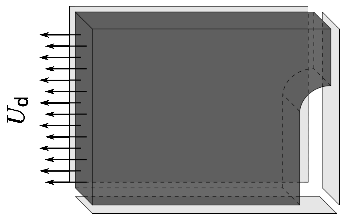
The different algorithms are tested in the case of a modified unified viscoplastic viscodamage model, in an infinitesimal strain settings, derived from [3,23,33,34]. The analysis is carried out on a three-dimensional plate made of Cr–Mo steel at $580{}^{°}\mathrm{C}$ [35] with a central groove. One-eighth of the plate with symmetric boundary conditions is shown in Figure 2. The plate geometry is defined by its length, width and depth being $(40,20,2)\mathrm{mm}$ while the length and width of the groove are $(10,4)\mathrm{mm}$. This plate is subjected to a uniformly distributed displacement field of the form $U_d=U_{0}sin\left(\frac{2\pi }{T}t\right)$ with t and T being the time and the time period, respectively.

Three examples are discussed below. Firstly, the effect of the temporal functions update is investigated; see Section 2.1. Then, the PGD behaviour with different orthonormalisation schemes is analysed to illustrate the optimality of the ROB. Lastly, the computational requirements of the orthonormalisation schemes and their effect on the temporal functions update are discussed.

4.1. POD-Like Temporal Functions Update

The analysis of the plate, shown in Figure 2, is carried out on a mesh that consists of 387 hexahedron elements, with eight integration points in each element, resulting in 1884 spatial displacement degrees of freedom. The model is subjected to a uniformly distributed displacement field with an amplitude $U_0=0.00606\mathrm{mm}$ and a time period $T=10\mathrm{s}$. The temporal discretisation is chosen such that the domain $[0,T]$ is discretised into 33 time steps. Since the whole time domain is computed at once, a total of $62,172$ degrees of freedom are being sought. The commonly used GS scheme (Algorithm 1) is utilised in this example and the convergence criterion is considered to be ${10}^{-10}$.

The purpose of this test case is to evaluate the importance of the updating step in a PGD approach. Hence, the number of generated modes along with the number of the LATIN iterations, with and without this POD-like step, is illustrated in Figure 3.

It is seen in Figure 3 that the required number of LATIN iterations is not affected by this updating step, but the computational cost is sharply decreased. Moreover, such a step is crucial to limit the size of the PGD expansion. With the updating step, only half the number of modes were generated in comparison with the approach without any update. Due to this favourable nature, the updating step is implemented in the rest of the examples.

4.2. PGD Behaviour with Different Orthonormalisation Schemes

The previous example with the same spatial discretisation is subjected to 12 load cycles with different amplitudes, in the range of $[0.0033,0.0066]\mathrm{mm}$. The temporal domain is divided into 12 intervals, each corresponding to one cycle, and the ROB generated within one cycle is reused in the following cycles. The convergence criterion is considered to be ${10}^{-4}$.

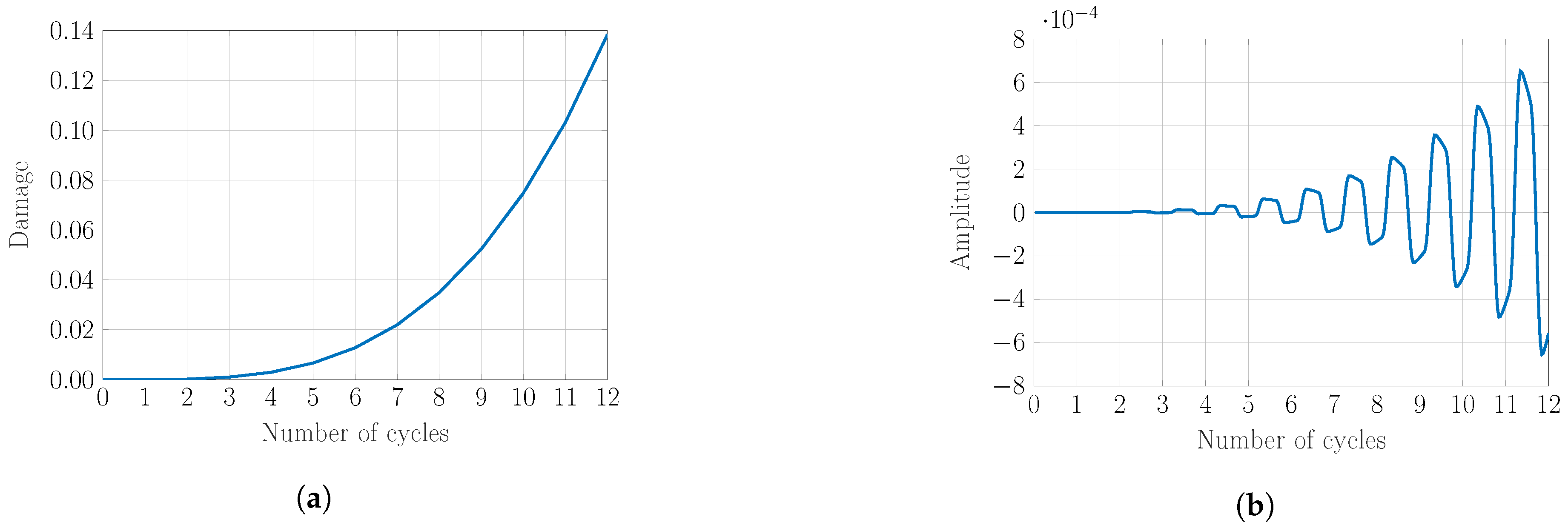
The nonlinearity and the rapid damage evolution can be seen in Figure 4a where the damage value at the end of each cycle is plotted with respect to the number of cycles. The first PGD temporal function of each cycle, after convergence, is illustrated in Figure 4b.

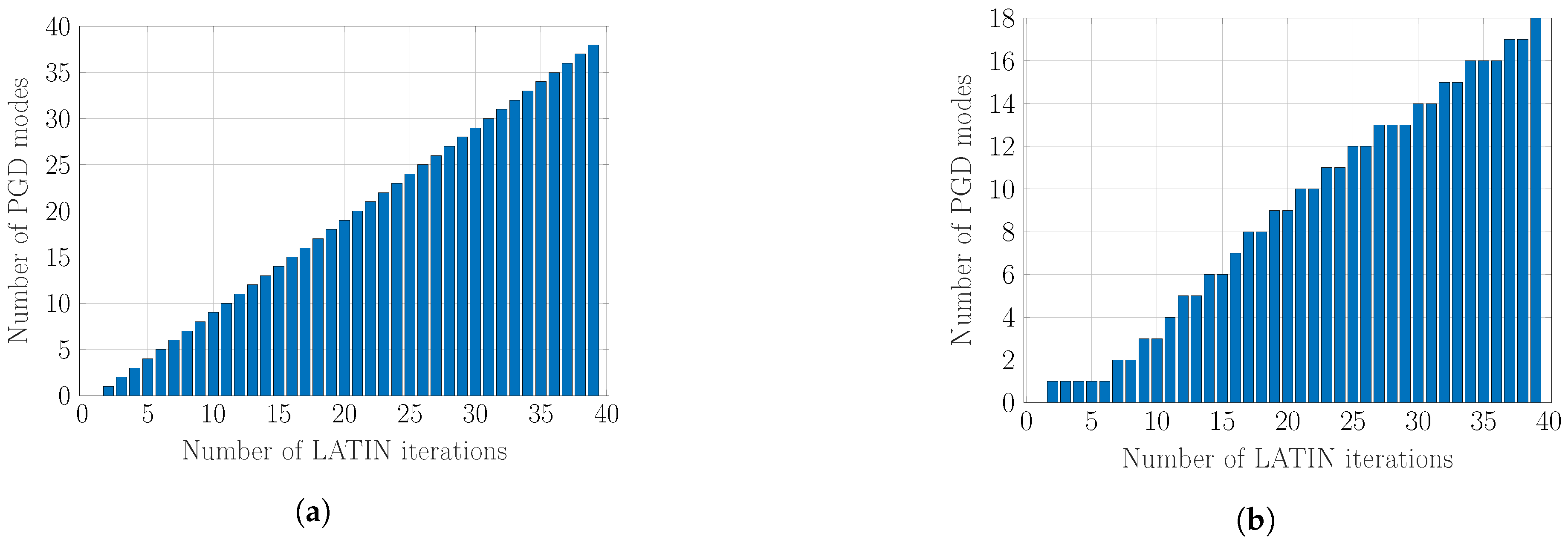
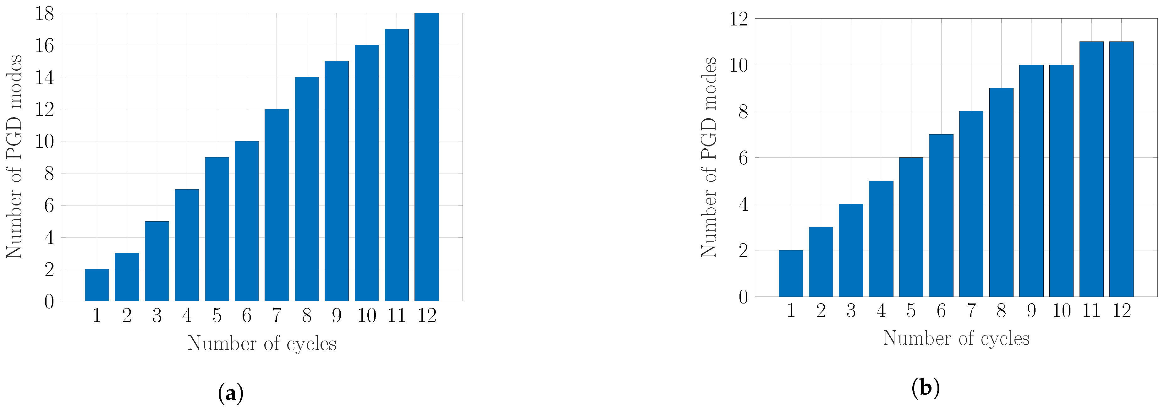
The simulation is carried out using Algorithms 1–4 and the resulting number of PGD modes with respect to the number of cycles is depicted in Figure 5. It is shown in Figure 5a that using Algorithm 1 resulted in an ROB with 18 modes while Algorithms 2–4 reduced this number to 11 modes by adding a maximum of one supplementary mode for each cycle. It is emphasised that Algorithms 2–4 provide the same ROB. However, their computational cost differs as illustrated in Section 4.3.

It is observed that an SVD compression provides optimality of the ROB. It also has interesting properties such as not rejecting any mode in the current example. In other words, due to the optimality of the generated ROB, the POD-like step plays a noticeable role in convergence and there is no need for further enrichment of the ROB.

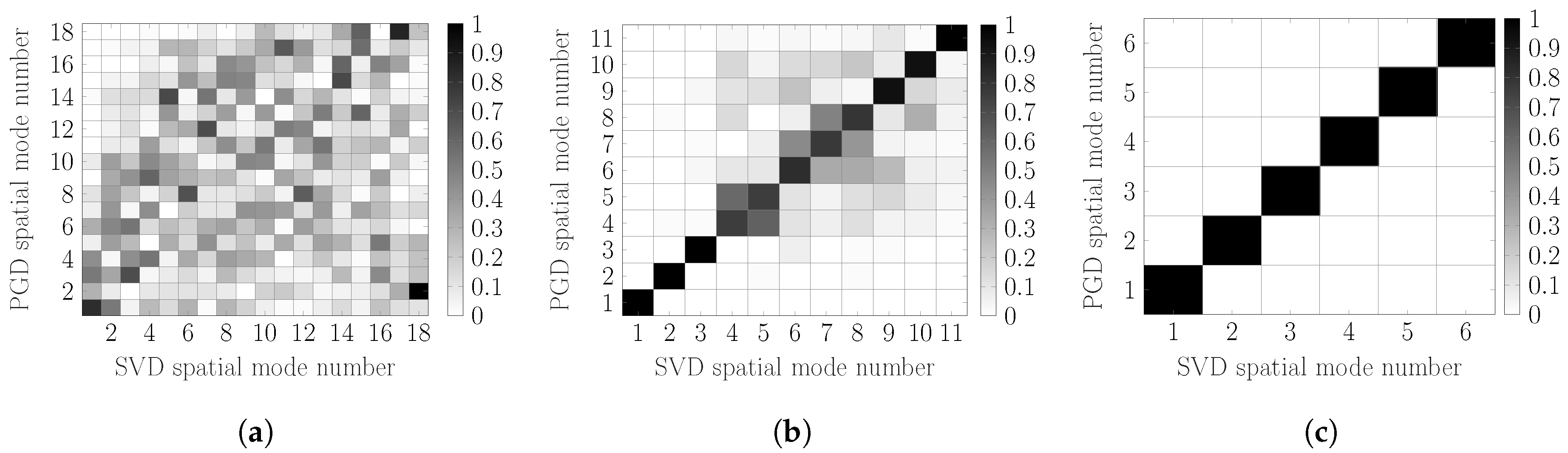
The inner product of the spatial modes in each case, after the last cycle, with their corresponding SVD of the acquired solution is shown in Figure 6. As expected, the GS modes are far from the optimal SVD ones while, trivially, Figure 6b depicts an almost diagonal matrix. The off-diagonal entries are caused by the temporal functions update at the final iterations.

It is of interest to point out that an excessive (R)SVD, termed e(R)SVD, step after the temporal functions update, which seems to be an unnecessary step, restricts the ROB to six modes only as illustrated in Figure 6c.

4.3. Relative Performance of the Different Orthonormalisation Schemes

The ensured optimality of the ROB is of interest when used with challenging examples such as in many-query context, due to the expected slow growth of the ROB. In order to investigate the robustness and the behaviour of the ROB, in a many-query context with a large number of degrees of freedom, the plate model is discretised into 13,812 hexahedron elements, with eight integration points in each element, resulting in $50,547$ spatial displacement degrees of freedom. The temporal discretisation consists of 33 time steps in each cycle resulting in $1,668,051$ degrees of freedom in each cycle. The plate is subjected to a uniformly distributed displacement field with a uniformly distributed random amplitudes in the range of $[18,22]\times {10}^{-5}\mathrm{mm}$ and a time period $T=10\mathrm{s}$. The convergence criterion is considered to be ${10}^{-4}$.

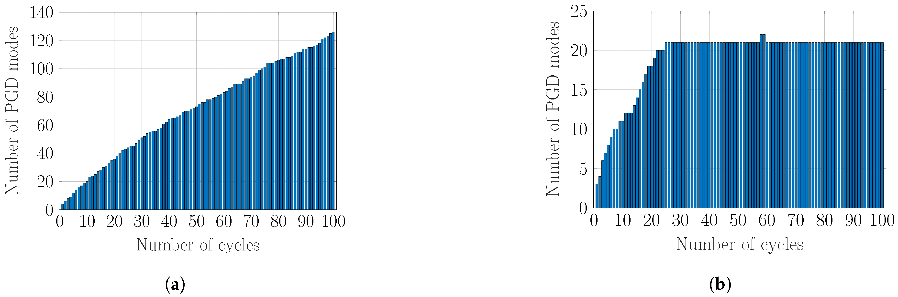
The resulting number of PGD modes with respect to the number of cycles using GS and SVD algorithms is illustrated in Figure 7 and Figure 8. It is seen that using a GS algorithm allows the ROB to grow to contain 126 pairs of modes while SVD algorithms confine this size to 21 modes, using a truncation threshold of ${10}^{-8}$. Accepting a bigger approximation error with a truncation threshold of ${10}^{-5}$ reduces the number of modes to 11 pairs while an e(R)SVD scheme introduces further reduction to seven modes without any rejection or truncation due to the maintained optimality of the ROB.

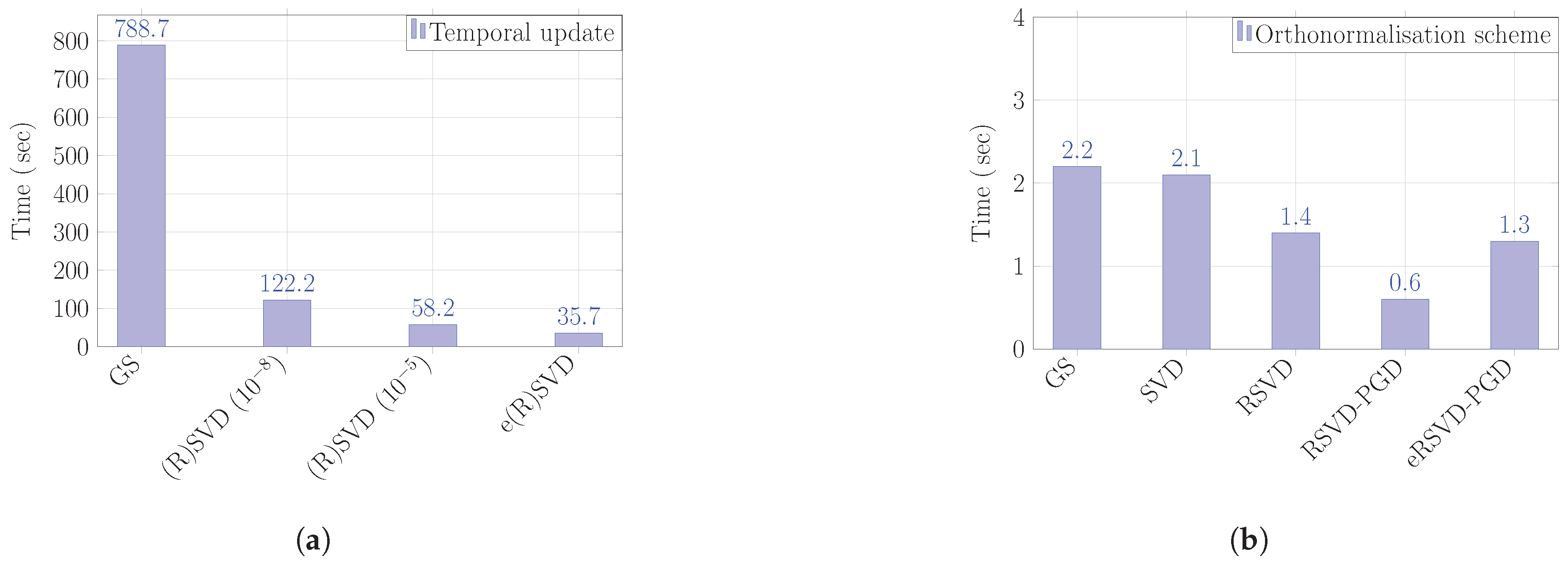
It is worth noting that, in this example, the SVD orthonormalisation schemes, other than e(R)SVD, were invoked 53 times only compared to 125 times with the GS algorithm. Hence, this explains the low computational requirements of Algorithms 2–4 in comparison with Algorithm 1 as summarised in Figure 9b. The e(R)SVD scheme was invoked in each LATIN iteration. However, due to the small number of generated modes, the required time to update the temporal functions is drastically decreased in comparison with the other schemes; see Figure 9a for a profiler summary.

It is worth noting that the timing for each algorithm depends on the available computational resources. However, we expect their relative performance not to change. The RSVD algorithm is implemented in MATLAB^® and uses its built-in SVD routine.

5. Conclusions and Further Research

Different orthonormalisation techniques were investigated to ensure the optimality of the PGD decomposition. These techniques and their effect on the PGD greedy algorithm are illustrated throughout examples with a varying number of degrees of freedom. It is found that a randomised SVD algorithm is a promising scheme to ensure the optimality of PGD expansions. It introduces beneficial time saving by limiting the number of modes compared to a Gram–Schmidt procedure and, at the same time, it shows a drastic speed-up compared to a deterministic SVD scheme. Another promising approach is proposed here where the randomised SVD scheme is invoked at each LATIN iteration, after the temporal update or the basis enrichment. This approach is referred to, in the current work, as e(R)SVD and it shows desired properties such as ensuring an optimal basis in each iteration and reducing the enrichment of basis functions to a minimum, i.e., no modes are rejected. The proposed numerical strategy, though it is presented in a LATIN-PGD framework, can be used to optimise PGD basis for any application.

References

- Chinesta, F.; Huerta, A.; Rozza, G.; Willcox, K. Model Reduction Methods. In Encyclopedia of Computational Mechanics; John Wiley & Sons: Hoboken, NJ, USA, 2018; Volume 3. [Google Scholar]
- Giacoma, A.; Dureisseix, D.; Gravouil, A.; Rochette, M. Toward an optimal a priori reduced basis strategy for frictional contact problems with LATIN solver. Comput. Methods Appl. Mech. Eng. 2015, 283, 1357–1381. [Google Scholar] [CrossRef] [Green Version]
- Bhattacharyya, M.; Fau, A.; Nackenhorst, U.; Néron, D.; Ladevèze, P. A LATIN-based model reduction approach for the simulation of cycling damage. Comput. Mech. 2018, 62, 725–743. [Google Scholar] [CrossRef]
- Niroomandi, S.; González, D.; Alfaro, I.; Bordeu, F.; Leygue, A.; Cueto, E.; Chinesta, F. Real-time simulation of biological soft tissues: A PGD approach. Int. J. Numer. Methods Biomed. Eng. 2013, 29, 586–600. [Google Scholar] [CrossRef] [PubMed]
- Heyberger, C.; Boucard, P.A.; Néron, D. A rational strategy for the resolution of parametrized problems in the PGD framework. Comput. Methods Appl. Mech. Eng. 2013, 259, 40–49. [Google Scholar] [CrossRef]
- Bhattacharyya, M.; Fau, A.; Nackenhorst, U.; Néron, D.; Ladevèze, P. A multi-temporal scale model reduction approach for the computation of fatigue damage. Comput. Methods Appl. Mech. Eng. 2018, 340, 630–656. [Google Scholar] [CrossRef]
- Cline, A.; Dhillon, I. Computation of the Singular Value Decomposition. In Handbook of Linear Algebra; CRC Press: Boca Raton, FL, USA, 2013; pp. 1027–1039. [Google Scholar]
- Chinesta, F.; Ladevèze, P. Separated Representations and PGD-Based Model Reduction; Springer: Vienna, Austria, 2014; Volume 554, p. 227. [Google Scholar]
- Kerfriden, P.; Gosselet, P.; Adhikari, S.; Bordas, S. Bridging proper orthogonal decomposition methods and augmented Newton–Krylov algorithms: An adaptive model order reduction for highly nonlinear mechanical problems. Comput. Methods Appl. Mech. Eng. 2011, 200, 850–866. [Google Scholar] [CrossRef] [PubMed] [Green Version]
- Ladevèze, P. Large time increment method for the analysis of structures with non-linear behavior caused by internal variables (La methode a grand increment de temps pour l’analyse de structures a comportement non lineaire decrit par variables internes). Comptes Rendus de l’Académie des Sciences. Série 2, Mécanique, Physique, Chimie, Sciences de l’Univers, Sciences de la Terre 1989, 309, 1095–1099. [Google Scholar]
- Ladevèze, P. On reduced models in nonlinear solid mechanics. Eur. J. Mech. A Solids 2016, 60, 227–237. [Google Scholar] [CrossRef]
- Nasri, M.A.; Robert, C.; Ammar, A.; El Arem, S.; Morel, F. Proper Generalized Decomposition (PGD) for the numerical simulation of polycrystalline aggregates under cyclic loading. Comptes Rendus Mécanique 2018, 346, 132–151. [Google Scholar] [CrossRef]
- El Halabi, F.; González, D.; Sanz-Herrera, J.A.; Doblaré, M. A PGD-based multiscale formulation for non-linear solid mechanics under small deformations. Comput. Methods Appl. Mech. Eng. 2016, 305, 806–826. [Google Scholar] [CrossRef]
- Ryckelynck, D. An a priori model reduction method for thermomechanical problems, Réduction a priori de modèles thermomécaniques. Comptes Rendus Mécanique 2002, 330, 499–505. [Google Scholar] [CrossRef]
- Ryckelynck, D. A priori hyperreduction method: An adaptive approach. J. Comput. Phys. 2005, 202, 346–366. [Google Scholar] [CrossRef]
- Giacoma, A.; Dureisseix, D.; Gravouil, A. An efficient quasi-optimal space-time PGD application to frictional contact mechanics. Adv. Model. Simul. Eng. Sci. 2016, 3. [Google Scholar] [CrossRef]
- Golub, G.H.; van Loan, C.F. Matrix Computations; The Johns Hopkins University Press: Baltimore, MD, USA, 2013. [Google Scholar]
- Bach, C.; Ceglia, D.; Song, L.; Duddeck, F. Randomized low-rank approximation methods for projection-based model order reduction of large nonlinear dynamical problems. Int. J. Numer. Methods Eng. 2019, 1–33. [Google Scholar] [CrossRef]
- Halko, N.; Martinsson, P.G.; Tropp, J.A. Finding Structure with Randomness: Probabilistic Algorithms for Constructing Approximate Matrix Decompositions. SIAM Rev. 2011, 53, 217–288. [Google Scholar] [CrossRef] [Green Version]
- Ladevèze, P. Nonlinear Computational Structural Mechanics; Springer: New York, NY, USA, 1999. [Google Scholar]
- Steinke, P. Finite-Elemente-Methode; Springer: Berlin/Heidelberg, Germany, 2015; p. 391. [Google Scholar]
- Felippa, C.A. Recent developments in parametrized variational principles for mechanics. Comput. Mech. 1996, 18, 159–174. [Google Scholar] [CrossRef] [Green Version]
- Lemaitre, J. A Course on Damage Mechanics; Springer-Verlag: Berlin/Heidelberg, Germany, 1992. [Google Scholar]
- Cueto, E.; González, D.; Alfaro, I. Proper Generalized Decompositions; Springer International Publishing: Cham, Switzerland, 2016. [Google Scholar]
- Chinesta, F.; Keunings, R.; Leygue, A. The Proper Generalized Decomposition for Advanced Numerical Simulations: A Primer; Springer International Publishing: Cham, Switzerland, 2014. [Google Scholar]
- Ladevèze, P.; Perego, U. Duality preserving discretization of the large time increment methods. Comput. Methods Appl. Mech. Eng. 2000, 189, 205–232. [Google Scholar] [CrossRef]
- Wunderlich, W.; Pilkey, W.D. Mechanics of Structures. Variational and Computational Methods. Meccanica 2004, 39, 291–292. [Google Scholar] [CrossRef]
- Gellin, S.; Pitarresi, J.M. Nonlinear analysis using temporal finite elements. Eng. Anal. 1988, 5, 126–132. [Google Scholar] [CrossRef]
- Allix, O.; Ladevèze, P.; Gilletta, D.; Ohayon, R. A damage prediction method for composite structures. Int. J. Numer. Methods Eng. 1989, 27, 271–283. [Google Scholar] [CrossRef]
- Bhattacharyya, M. A Model Reduction Technique in Space and Time for Fatigue Simulation. Ph.D. Thesis, Leibniz Universität Hannover, Hannover, Germany, 2018. [Google Scholar]
- Bebendorf, M. Hierarchical Matrices; Springer-Verlag: Berlin/Heidelberg, Germany, 2008; Volumn 63, pp. 1–302. [Google Scholar]
- Eckart, C.; Young, G. The approximation of one matrix by another of lower rank. Psychometrika 1936, 1, 211–218. [Google Scholar] [CrossRef]
- Chaboche, J.L.; Nouailhas, D. A Unified Constitutive Model for Cyclic Viscoplasticity and Its Applications to Various Stainless Steels. J. Eng. Mater. Technol. 1989, 111, 424. [Google Scholar] [CrossRef]
- De Souza Neto, E.A.; Peric, D.; Owen, D.R.J. Computational Methods for Plasticity: Theory and Applications; John Wiley & Sons: Hoboken, NJ, USA, 2011. [Google Scholar]
- Lemaitre, J.; Desmorat, R. Engineering Damage Mechanics; Springer-Verlag: Berlin/Heidelberg, Germany, 2005. [Google Scholar]
Figure 1.
Graphical representation of the strong form of a structural problem (Tonti Diagram).
Figure 2.
A plate with a central groove subjected to cyclic loading.
Figure 3.
The size of the generated ROB. (a) ROB size without the updating step; (b) ROB size with the updating step.
Figure 4.
Damage evolution and the first PGD temporal mode in each cycle. (a) damage w.r.t. number of cycles; (b) first temporal function.
Figure 5.
Number of PGD modes in each cycle using different orthonormalisation schemes. (a) number of PGD modes using GS; (b) number of PGD modes using (R)SVD.
Figure 6.
ROB optimality w.r.t. an SVD of the resulting solution. (a) GS; (b) (R)SVD; (c) e(R)SVD.
Figure 7.
ROB size using different orthonormalisation algorithms. (a) number of PGD modes using GS; (b) number of PGD modes using (R)SVD ().
Figure 8.
ROB size using different orthonormalisation algorithms. (a) number of PGD modes using (R)SVD (); (b) number of PGD modes using e(R)SVD.
Figure 9.
The required time to perform the temporal update and the orthonormalisation steps. (a) timing of the temporal functions update; (b) timing of orthonormalisation schemes.