The Application of Stock Index Price Prediction with Neural Network


1
Department of Mathematical Sciences, Xi’an Jiaotong-Liverpool University, Suzhou 215123, China
2
Department of Computer Science and Software Engineering, Xi’an Jiaotong-Liverpool University, Suzhou 215123, China
*
Author to whom correspondence should be addressed.
Math. Comput. Appl. 2020, 25(3), 53; https://doi.org/10.3390/mca25030053
Submission received: 6 July 2020
/
Revised: 16 August 2020
/
Accepted: 16 August 2020
/
Published: 18 August 2020
(This article belongs to the Special Issue Intelligent Computation and Its Applications in Financial Technology)
Abstract
:Stock index price prediction is prevalent in both academic and economic fields. The index price is hard to forecast due to its uncertain noise. With the development of computer science, neural networks are applied in kinds of industrial fields. In this paper, we introduce four different methods in machine learning including three typical machine learning models: Multilayer Perceptron (MLP), Long Short Term Memory (LSTM) and Convolutional Neural Network (CNN) and one attention-based neural network. The main task is to predict the next day’s index price according to the historical data. The dataset consists of the SP500 index, CSI300 index and Nikkei225 index from three different financial markets representing the most developed market, the less developed market and the developing market respectively. Seven variables are chosen as the inputs containing the daily trading data, technical indicators and macroeconomic variables. The results show that the attention-based model has the best performance among the alternative models. Furthermore, all the introduced models have better accuracy in the developed financial market than developing ones.
1. Introduction
The stock market is an essential component of the nation’s economy, where most of the capital is exchanged around the world. Therefore, the stock market’s performance has a significant influence on the national economy. It plays a crucial role in attracting and directing the distributed liquidity and savings into optimal paths. In this way, the scarce financial resources could be adequately allocated to the most profitable activities and projects [1]. Investors and speculators in the stock market aim to make better profits from the analysis of market information. Thus, one could take advantage of the financial market if they have proper models to predict the stock price and volatility which are affected by macroeconomic factors, and also by hundreds of other factors.
The stock index price prediction has always been one of the most challenging tasks for people who work in the financial field and other related scales due to the volatility and noise features [2]. How to improve the accuracy of the stock index price prediction is an open question in modern society. The definition of time series can be summarized as a chronological sequence consisting of observed data from discretionary periodical behavior or activity in some fields such as social science, finance, engineering, physics, and economics. The stock index price is a kind of financial time series which has a low signal-to-noise ratio [3] and heavy-tailed distribution [4]. Those kinds of complicated features make it very tough to predict the trend of the index price. Time series prediction aims at building models to simulate the future values given their past values. As in many cases, the relationships between past and future observations is not deterministic, this amounts to expressing the conditional probability distribution as a function of the past observations [4,5]:
There are many traditional econometric models for forecasting time series such as the Autoregressive (AR) Model [6], Autoregressive Moving Average (ARMA) Model [7], Generalized Autoregressive Conditional Heteroskedasticity (GARCH) Model [8], Vector Autoregressive model [9] and Box–Jenkins [10] which have nice performance in predicting stock price. In the past decade, deep learning has experienced booming development in many fields. Deep learning has a better explanation on the nonlinear relationships than other traditional methods. The importance of nonlinear relationships in financial time series has gained much more attention in researchers and financial analysts. Therefore, people start to analyze the nonlinear relationships by using deep learning methods such as Artificial Neural Networks (ANNs) [2,11] and Support Vector Regression (SVR) [12,13], which have been applied in financial time series prediction and have good predictive accuracy. However, a deep nonlinear topology that should be applied to predict time series raises the consideration in the recent trend in the communities of pattern recognition and machine learning. Considering the complexity of financial time series, combing deep learning methods with financial market prediction is regarded as one of the most charming topics in the stock market [14,15,16]. The main aim of using deep learning is to design an appropriate neural network to estimate the nonlinear relationships representing f in Equation 1. Nevertheless, this kind of field remains a less explored area.
In this paper, we aim to make a comparison in the stock index price prediction by using three typical machine learning methods and Uncertainty-aware Attention (UA) mechanism [17] to testify the prediction performance. We will build four models to predict the stock index price: Multilayer Perceptron (MLP), Long Short Term Memory (LSTM), Convolutional Neural Networks (CNN), and Uncertainty-aware Attention (UA).
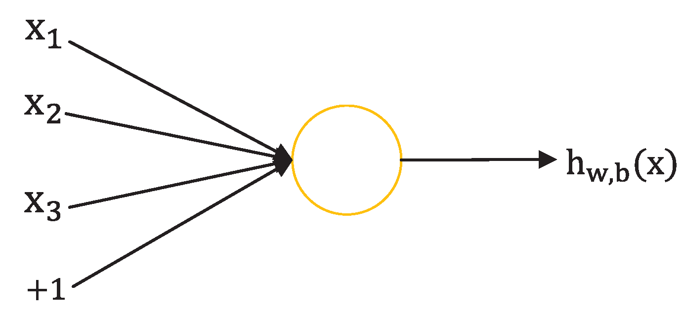
Neural networks are widely parallel interconnected networks composed of simple adaptive units whose organization can simulate the interaction of biological nervous systems with real-world objects [18]. In biological neural networks, each neuron is connected to other neurons, and when it is excited, it sends chemicals to the connected neurons, changing the potential within those neurons. If the potential of a neuron exceeds a threshold, then it will be activated and sends chemicals to other neurons. When we abstract this neuron model out, for example, it can be described as the M-P network with one neuron and three input nodes. In Figure 1, we can see that the neuron receives input x and transmits through the connection with weight w. Then it compares the total input signal with the neuron threshold, and determines whether it is activated through activation function processing.
Making use of neural architecture, artificial neural networks (ANNs) has been through rapid development in the past few decades. ANNs could learn and generalize from experience with building complex neural network to deal with the non-linear relationships among complex time series, which makes it a good approximator in forecasting problems. Multi-layer Perceptron is a feedforward artificial neural networks. One MLP consists of, at least, three layers of nodes: An input layer, a hidden layer and an output layer [19]. Except for the input nodes, each node is a neuron that uses a nonlinear activation function. MLP utilizes a supervised learning technique called backpropagation (BP) for training [20]. Its multiple layers and non-linear activation distinguish MLP from a linear perceptron. It can distinguish data that is not linearly separable [21]. Long Short Term Memory (LSTM) is a particular type of Recurrent Neural Network (RNN). LSTM was first proposed in 1997 by Sepp Hochreiter and Jürgen Schmidhuber [22] and improved in 2000 by Felix Gers’ team [23]. This kind of neural network has great performance in learning about long-term dependencies. A common LSTM unit is composed of a cell, an input gate, an output gate and a forget gate [22,23]. The cell remembers values over given time intervals and the three gates regulate the flow of information into and out of the cell. LSTM is very popular in image processing, text classifying, and time series predictions. LSTMs were developed to deal with the exploding and vanishing gradient problems that can be encountered when training traditional RNNs. Convolutional Neural Network (CNN) is usually applied in the pattern recognition which is designed according to the visual organization of the human brain. CNN consists of convolution layer, pooling layer and fully connected layer with nonlinear activation function between each layer. The network utilizes a mathematical operation called convolution which is a specialized linear operation in place of general matrix multiplication. CNN has unique advantages dealing with processing image problems due to its special structure of local weight sharing reducing the complexity of the network. UA is an attention-based model using RNN as its basic structure. The network employs two RNNs dealing with the raw time series data and generates temporal attention and variable attention in terms of time and feature using variational inference. This special design could reflect the connection among different variables better.
In this work, four methods would be used to predict the stock index price and we would compare the performance among the alternative models.
2. Literature Review
Literature in time series prediction has a long history in finance and econometric. In this part, some related work will be introduced in terms of machine learning since artificial intelligence gains a booming development, which inspires the idea to this paper.
As is known, both macroeconomic factors and financial series inherent changes can influence the stock index price. Xiong et al. applied Long Short Term Memory neural network to model SP500 index volatility with Google domestic trends as the indicators of the macroeconomic factors [24]. Forecasting the implied volatility is also crucial in stock price predicting. Except for the high, low, open and close price data, they collect 25 domestic trends which could be considered as a representation of the public interest together as the input data. In their work, the group uses the mutual information method to determine the value of the observation interval and the normalization window size. As for the benchmark, they use the GARCH model as a comparison with the LSTM model. Results show that the LSTM model performs better than the GARCH model.
In the work of Hiransha, M et al. the group applied four types of neural networks named MLP, RNN, LSTM, and CNN to test the performance on predicting two stock markets price [25]. The dataset is taken from NSE market including three different sectors of Automobile, Banking and IT. The NYSE market contains the Finance and Petroleum sectors. ARIMA model was used in this article as the comparison between linear and nonlinear models.
There are many improvements that could be made in the model predicting performance in the option trading markets. While traditional closed-form models such as the Kemna–Vorst Model and Levy Approximation are widely used and performed well, the accuracy needs to be improved. Zhou and George proposed a model to improve the accuracy of option pricing by using neural network integrated with Levy Approximation [26]. First, the authors used the Antithetic Monte Carlo model to obtain a better forecasting result as the benchmark of learning. Second, the implied volatility of the Levy Approximation model was modified with Monte Carlo prices. Third, a neural network was built to map the real volatility to the implied volatility.
The price in the stock market has already reflected all known information which means that the financial market is ‘informationally efficient’ [27] and the price is influenced by news or events. Ding et al. made use of the work in Natural Language Processing (NLP) and applied this in the stock market prediction [28]. In this article, the team proposed a novel deep neural network in the event-driven stock market prediction. The experimental results show that the proposed model could achieve almost 6% improvements compared with state-of-the-art baseline methods.
Bao et al. proposed a novel deep learning framework combining wavelet transforms (WT), stacked autoencoders (SAEs) and LSTM in stock price prediction [29]. There are three stages in this model. First, the WT method was used to eliminate noise by decomposing the stock price series. Haar function was used as the wavelet basis function due to its ability in decomposing the financial time series and reducing the processing time significantly [30]. Second, after denoising the time series data, SAEs which is unsupervised layer-wise training was applied to extract the deep features from input data. Single AE is a three-layer neural network including input layer, hidden layer and output layer also called reconstruction layer. This architecture aims at minimize the error between the input layer and the reconstruction layer through the hidden layer designed to get the deep features. The authors used four single-layer autoencoders and every AE was trained with the same gradient descent algorithm. Lastly, LSTM was introduced to forecast the stock price using the processed time series with high-level features which were the last hidden layer output in the second part. The efficiency of solving vanishing gradients and learning long-term dependency in LSTM could help to predict stock price better.
In the work of Chen et al. [31], they proposed an eight-layers convolutional neural network. The main task of this work is to make the binary classification instead of predicting exact values. The output of this model contains two values–one or zero representing the stock price movement–up or down. They used 1D convolution since the stock price data belonged to the 1D time series. Result shows that CNN could have decent performance as well as RNN in time series predicting.
Binkowski et al. proposed a novel convolutional network in predicting multivariate asynchronous time series called Significance-Offset Convolutional Neural Network (SOCNN) [2]. This model is designed as a combination of the AR model and CNN. The authors were inspired by the gate mechanism in RNN. The output of this model is obtained as a weighted sum of adjusted coefficients which depend on input data parameterized through a convolutional network. There are two convolutional parts in this model architecture. One captures the local significance of observed data while the other represents the predictors that are completely independent of position in time. The combination could learn both the information of raw time series and the weighs in the AR system.
Traditional CNN in dealing with time series might not reflect the information in terms of time domain properly. Thus Lea et al. introduced a novel temporal model called Temporal Convolutional Networks (TCN), which used a hierarchy of temporal convolutions to perform fine-grained action segmentation or detection [32]. The main task is time series classification. The authors designed an encoder-decoder TCN structure with hierarchy of temporal convolutional filters which could capture long-range temporal patterns prominently. The parameters in the network will be updated simultaneously in every time step and the convolution is computed across time [32]. The proposed TCN model could have faster speed in training network than LSTM-based recurrent neural networks.
Qin et al. proposed a dual-stage attention-based recurrent neural network (DA-RNN) to address the limits that traditional methods could not capture the long-term temporal dependencies appropriately and select the relevant driving series to make predictions [33]. In the first stage, the authors extract the endogenous series at each time step that affects the outcome most with a new attention mechanism by referring to the previous encoder hidden state. In the second stage, the model will automatically select relevant encoder hidden states with the designed temporal attention mechanism across all time steps. Through the two attention mechanisms in encoder and decoder separately, this model could learn the long-term temporal dependencies and choose the most related input variables of a time series.
3. Methodology
3.1. Multilayer Perceptron
Multilayer Perceptron (MLP) is a kind of primary artificial neural network which consists of a finite number of continuous layers. One MLP at least has three layers including input layer, hidden layer, and output layer. In many cases, there could be more hidden layers in the MLP structure which can deal with approximate solutions for many complex problems such as fitting approximation. One MLP can be thought of as a directed graph mapping a set of input vectors to a set of output vectors, which consists of multiple node layers connected to the next layer. These connections are generally called links or synapses [34]. In addition to the input nodes, each node is a neuron with a nonlinear activation function. A supervised learning method (BP algorithm) called backpropagation algorithm is often used to train MLP. MLP is a generalization of the perceptron, which overcomes the weakness that the perceptron can’t recognize inseparable linear data. The layers of MLP are fully connected, which means every neuron of each layer is connected with all neurons of the previous layer, and this connection represents a weight addition and sum. Figure 2 shows the framework of MLP model.
In detail, from the input layer to the hidden layer: X represents the input and represents the first hidden layer, then the formulation is , where stands for weight parameters and stands for bias parameters, and the function f is usually a non-linear activation function. During the hidden layers, it repeats the similar methods to get the hidden layers’ output. Every layer has different weight parameters and bias parameters. From hidden layer to output layer, Y is used to represent the output, then , stands for the last hidden layer and L stands for the number of the hidden layer. The function G is the activation function, commonly known as Softmax. Therefore, the relationships between input and output will be built. If the weight w or bias b of one neuron or several neurons are changed a little bit, the output of that neuron will be different, and those differences will eventually be reflected in the output. Finally, BP algorithm and optimization algorithm are used to update the weight W and bias B to get the expected results.
3.2. Long Short Term Memory
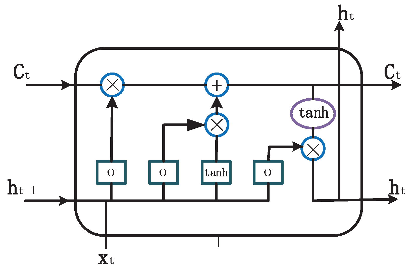
Long Short Term Memory (LSTM) is a particular Recurrent Neural Network (RNN), which successes the superiority of RNN and has better performance with long-term dependency applied in many fields [22]. Due to the vanishing gradient problem, RNN has difficulty in learning long-term dependencies [35]. LSTM is a practical solution for combating vanishing gradients by using memory cells [22,23]. All recurrent neural networks have a repeated chain in one single neural cell. Traditional RNN only has one layer in the neural cell, but LSTM has four layers which are particularly interacting with each other. The key to LSTM is the cell state . Cell state is like a conveyor belt that runs through the chain, with only linear interaction, keeping information flow unchanged. LSTM can delete or modify the information of the cell state, which is regulated by the gate mechanism. The gate mechanism is a way for information to pass selectively, consisting of the sigmoid neuronal layer and the pointwise multiplication operation. There are three types of gates in the LSTM cell to protect and control cell state. Every gate has an expression of . The range of sigmoid layer output is (0,1), which indicates how much of each component in should be passed. If the output is 0, it means that no pass is allowed while the output of 1 representing all pass. Figure 3 shows the framework of LSTM model.
3.2.1. Forget Gate Layer
The first step of LSTM is to decide what information to discard from the cell state. This decision is made by a sigmoid layer called the ‘forget gate layer’. It will output a vector ranging from 0 to 1 for cell state according to and . If the value equals to 1, it means to keep the whole information from , while 0 indicating dropping the information completely. Here represents the value of the forget gate.
3.2.2. Input Gate Layer
The second step is to decide what new information should be stored in cell state, which consists of two parts:
- (1).
- One sigmoid layer determines what kind of values should be updated represented as .
- (2).
- One tanh layer will create a new candidate value of which will be added to the state information.
Flowing, the two values of and will be combined to update the state. After that, the state by adding two items with and will be updated as Equation 3. Here, the symbol ∗ represents the element-wise product.
3.2.3. Output Gate Layer
Lastly, the output is going to be determined by the output gate layer, which is based on the cell state. The hidden state is the element-wise product of a tanh activation layer of and output gate capturing the information of previous hidden state and input .
One fully connected layer will be applied to generate the final predictions based on the hidden states h.
3.3. Convolutional Neural Network
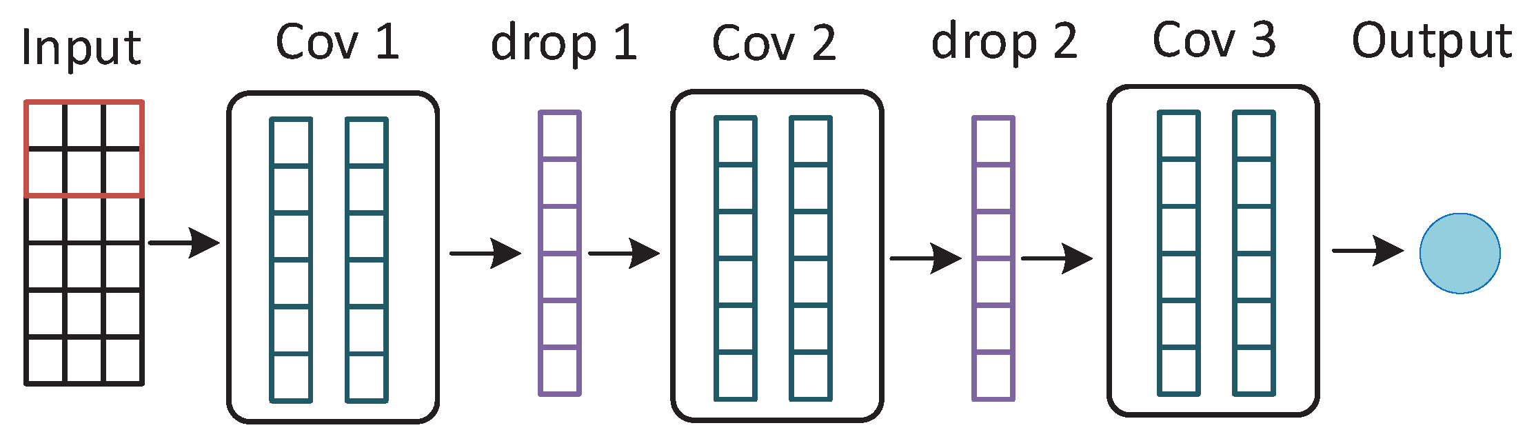
Convolutional Neural Network (CNN) is a typical deep neural network inspired by the human visual nervous system. CNN is usually applied in image processing. For multivariate time series prediction, CNN could be applied to deal with the 2-D input time series data. CNN has two important properties to reduce the number of parameters. The first one is called the local perceptron. Each neuron perceives the local information and then combine the local information at a higher level to obtain the global information like the human brain. The second one is called weight sharing. Each neuron acts as a filter to extract the local features from local input data. The filter slides through the image until all the data points in one image are covered with fixed window size. There are three main layers in a convolutional neural network. Figure 4 shows the framework of CNN model.
Convolution layer is the core of CNN. The convolution kernel also called filter could be considered as a small window that contains learned parameters as a matrix form. This filter slides all over the input data to capture the local information by applying the convolution operation on each patch. Different local information by applying different convolution kernels would be combined to generate the global information.
Pooling layer is added between continuous convolution layers in one CNN structure. It is designed to gradually reduce the amount of data and parameters, which could help to avoid overfitting to some extent. The pooling layer utilizes a small sliding window which is similar to the convolution layer. The convolved features of a specific area are compressed into the maximum value or the mean value of that area.
Fully connected layer is applied after several convolution layers and pooling layers to obtain the prediction results or classification results. The latent features through dimensionality reduction and feature extraction would be learned well with a fully connected layer.
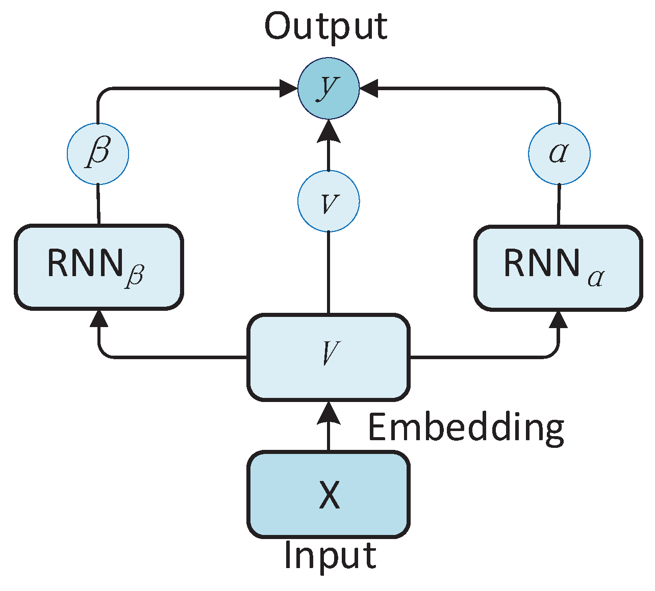
3.4. Uncertainty-Aware Attention
Uncertainty-aware Attention (UA) is proposed by [17]. UA is an attention-based model that utilizes two RNNs to generate two types of attentions. The attention mechanism was originally applied in image processing. It simulates the visual mechanism of human brains that people will focus on some special areas when they watch the whole picture. This indicates that the human brain’s attention to the whole picture is not balanced, which has a certain weight distinction. UA makes use of variational inference to learn this mechanism. Specifically, the two types of attention weights are assumed as Gaussian distribution with input dependent noise, and produced with two RNNs. The model generates attentions with small variance when it is confident about the contribution of the given features, and allocates noisy attentions with large variance to uncertain features for each input. With the input embeddings , the two different attentions w.r.t timesteps () and features () are generated follow the below equations:
The parameters of two RNNs are represented as and i is the timestep we are interested in. The two attentions are produced through squashing functions Softmax and tanh, respectively, with the attention logits and which are generated from the RNN outputs and . Then the context vector would be obtained by a convex sum of attentions , and embedding : . One fully connected layer would be applied to generate the final predictions: , where represents the fully connected layer. Figure 5 shows the framework of UA model.
4. Experiments and Results
4.1. Dataset
In this paper, three stock indices would be chosen from three different markets which represent three different market levels as our datasets. Eight years time period has been collected in these datasets which are from July 2008 to September 2016. In the real world, the market state may have the potential influence on the validity of our model prediction. It would be helpful to build the model if we choose datasets from different market conditions.
For the datasets, the first one for analysis is the CSI300 index from mainland China which is considered as a developing market. In this kind of market, there are many issues that the institutions should complete to improve the financial mechanism gradually. The second one is the S&P500 index from the US trading market in New York stock exchange, which is considered as the most advanced financial market. This kind of market is at the highest development level. Thus we choose the S&P500 index representing the most developed market. The third one is the Nikkei225 index from Tokyo financial market which represents the state between developed and developing market. These three different stock indices could help us test the robustness of the model prediction.
In these three different markets, we choose seven variables as our inputs and divide them as three sets. Table 1 shows the details about the selected variables.
The first set is historical trading data of each index including open price, close price and trading volume. Those kinds of variables represent the necessary trading information. The second part is technical indicators consisting of Moving Average Convergence Divergence (MACD) indicator and Average True Range (ATR) indicator. The third set is the macroeconomic variables including exchange rate and interest rate. In general, macroeconomic factors may have a significant impact on the performance of the stock markets. According to Zhao, the authors conclude that the fluctuation of currency exchange rate could have an essential influence on the trend of stock markets [36]. Therefore, the exchange rate and interest rate would be the first choice as extra inputs in the model prediction which may explain more potential information in stock prediction. In this paper, the US dollar index have been used as the proxy for the exchange rate which is the most crucial role in the monetary market. As for interest rate, we select Shanghai Interbank Offered Rate (SHIBOR) in mainland China market, Tokyo Interbank Offered Rate (TIBOR) in the Tokyo market and Federal funds rate of the US.
4.2. Experimental Design
In this section, the performance of each model would be discussed in the experimental and evaluation aspects.
4.2.1. Prediction Approach
The data is divided into two parts: The training part which is used to train the model and update the model parameters, the other part which would be used for testing part so that we would use the data to optimize the model for data forecasting. For all methods, 90% of the data are used to train the models and 10% of the data are used to test the performance of the models. Figure 6 shows the three different market indices’ close price.
According to this figure, we could see that the original time series of the three markets are not stationary. For deep learning methods, there is no need for the time series to be stationary. For all methods in this paper, the index’s close price of the next day is used as the label to make predictions and seven features described in the dataset section before are chosen as the input variables. For the MLP model, we design for four hidden layers with the corresponding neurons 70, 28, 14, 7 in each hidden layer and one fully connected layer as the output layer. For hidden layers, the activate function is relu function. In the LSTM model, the unit of hidden layer is designed to be 140. One fully connected layer is chosen as the output layer. Sigmoid function and tanh function are used in the LSTM cell. For the CNN model, we choose three convolution layers with the corresponding channels 7, 5, 3. Each convolution layer has the same kernel size of 3. We apply drop layer after each convolution layer. In the UA model, the hidden units of two RNNs are set to be 70. The embedding size of v is 7. One fully connected layer is used to output the final predictions. Table 2 shows the hyper-parameters of each method. For all methods, the time step is set to be twenty and learning rate is 0.01. We choose Mean Square Error (MSE) loss as our loss function and use Adam algorithm to optimize the loss function. The batch size is set to be 64. All the input data will be shuffled before training. The experiments of all methods were implemented on PyTorch.
4.2.2. Predictive Performance
In this part, the accuracy measurements would be introduced which are designed to compare the performance of the four different models. Here, we choose three classical indicators including Mean Absolute Percentage Error (MAPE), Root Mean Square Error (RMSE), and Correlation Coefficient (R) as the measurements for the predictive performance of each model. The equation of each indicator is shown in the following section:
In the above equations, is the original series that we want to forecast and is the mean of the original series. is the predicted series obtained from the model output and is the mean of the predicted series. N represents the number of samples in one batch. Among the three indicators, MAPE measures the size of the error calculated as the relative average of the error, and RMSE measures the mean square error of the true values and the predicted values. R is a measure of the linear correlation between two variables. Here, the model would perform well with smaller MAPE and RMSE. The predicted series is similar to the actual series with larger R.
4.3. Results
Table 3 shows the summarized experimental results of all methods on the three different market index price datasets. The best performance is displayed in boldface. In general, the UA model outperforms the other three models in all metrics, which indicates that the attention-based model could achieve better performance in multivariate financial time series prediction. The attention mechanism could allocate more contribution to a specific variable which has more impacts on the predictions.
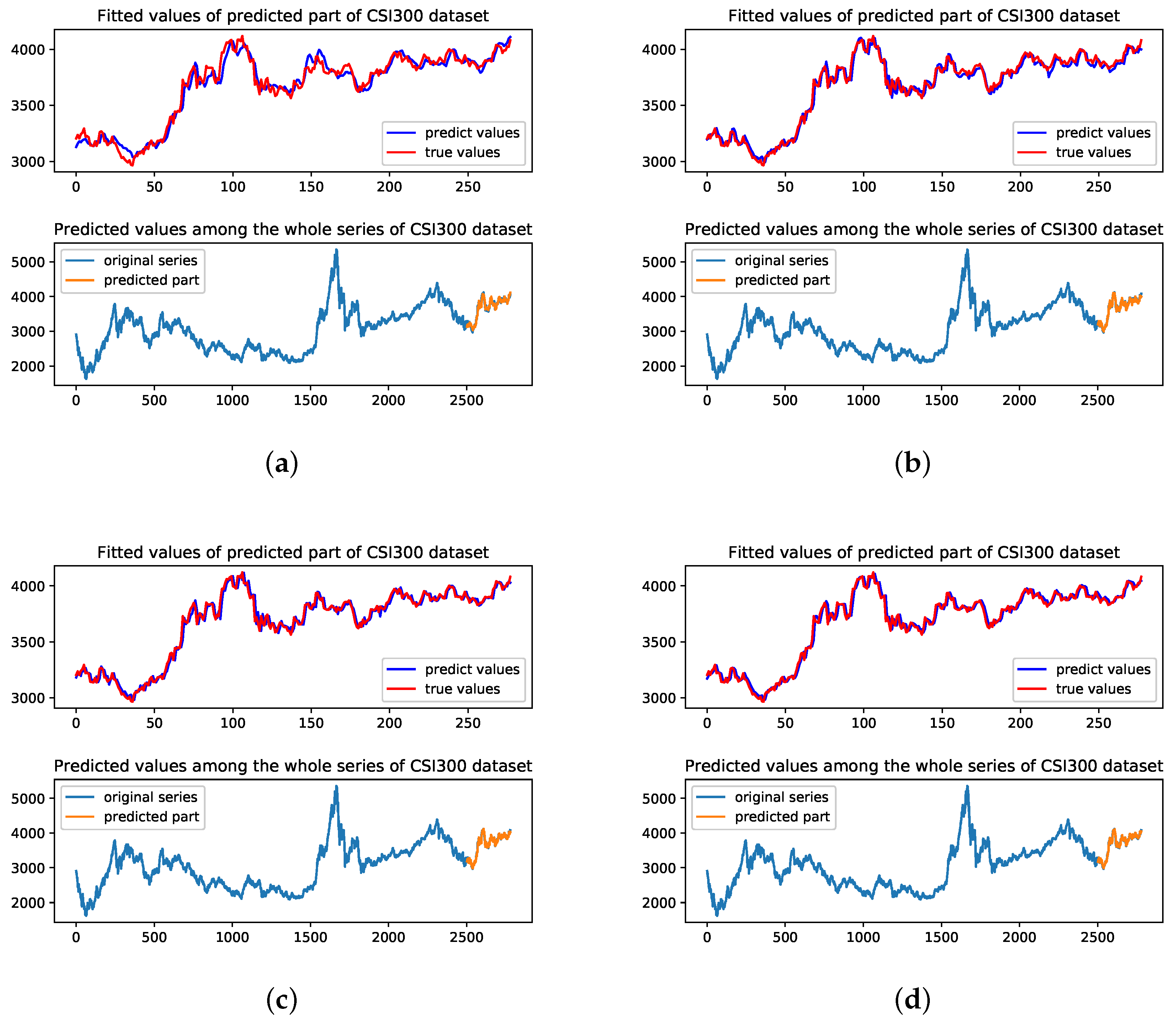
MLP model has the worst performance on the three datasets. This is mainly because MLP is a simple neural network only with several fully connected layers. This simple structure would limit the model prediction with multivariate time series. LSTM model performs well in CSI300 dataset which represents the developing financial market, while not perfect in the other two datasets. LSTM model has similar results on RMSE and R indicators with UA model on CSI300 dataset which are better than MLP model. Figure 7 shows the predicted results of four methods on the CSI300 dataset.
The top figure represents the fitted value of the forecasting period and the bottom figure represents the prediction results among the whole time series on each method.
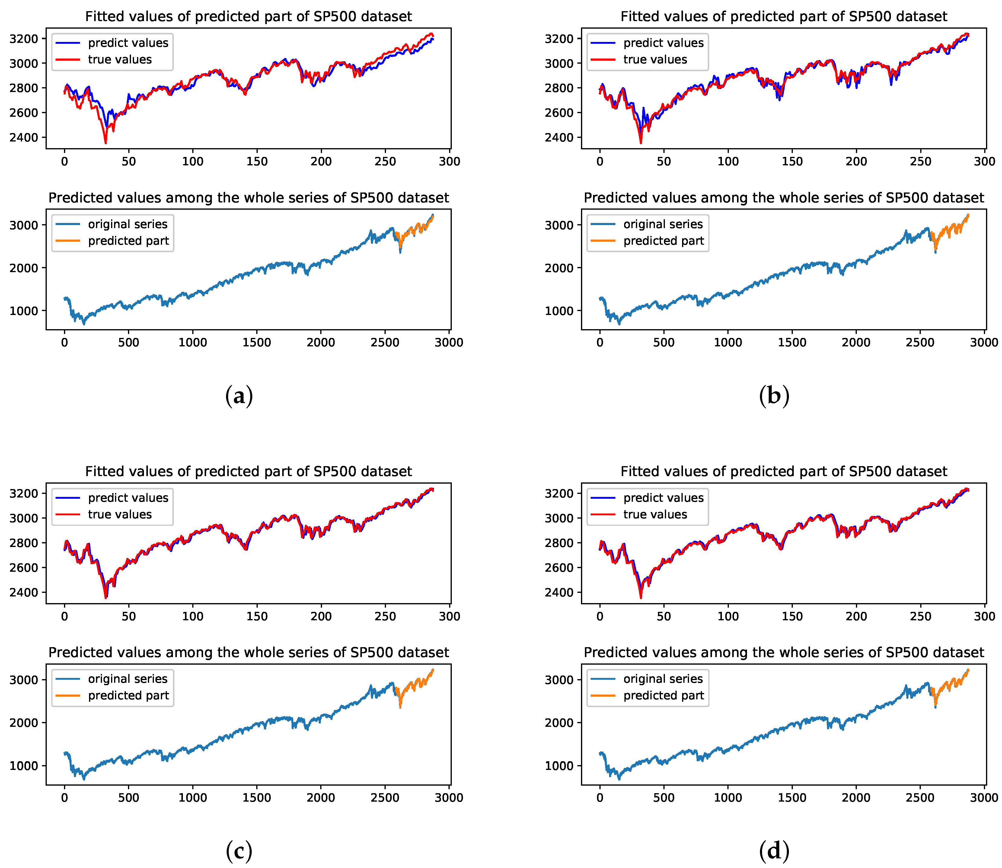
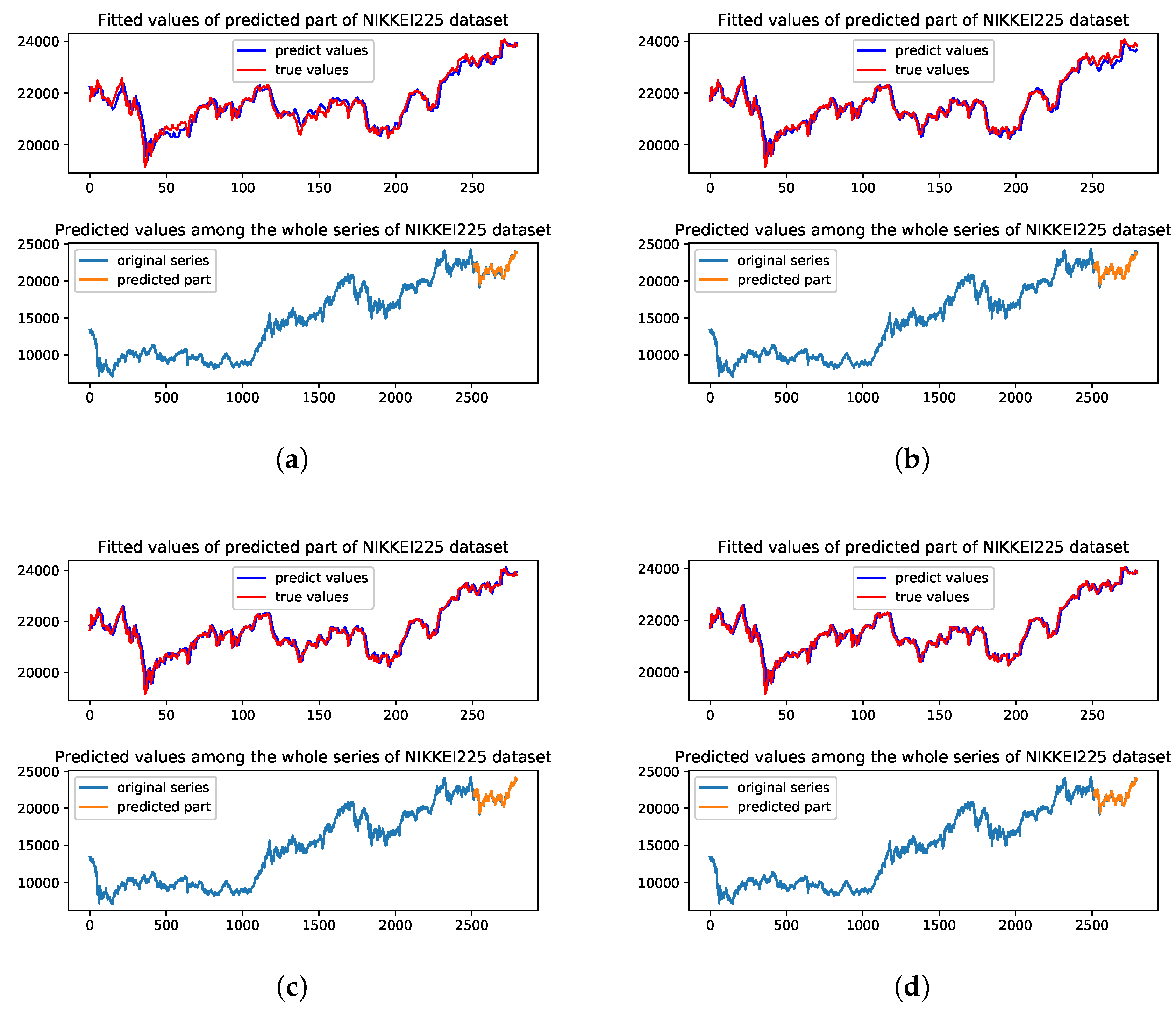
We could see that the LSTM model has smaller volatility at the end of the forecasting period. In Figure 7d, the UA model has better fitted results of the original series in the forecasting period. This reflects that RNN based structure could handle less complete financial market time series properly. As for SP500 dataset and Nikkei225 dataset, CNN and UA models perform similarly. UA model has smaller RMSE, MAPE and bigger R on both SP500 index and Nikkei225 index which represent the most developed financial market and less developed financial market, respectively. Figure 8 and Figure 9 show the predicted results of four methods on SP500 dataset and Nikkei225 dataset, respectively.
Through the results of different datasets representing different market stage, we find that all the four models perform differently in the financial market with the different economic states from Table 3 and Figure 7, Figure 8 and Figure 9. As for the UA model, the SP500 index has the smallest MAPE of 0.0067 which is much smaller than CSI300 index and Nikkei225 index with MAPE of 0.0071 and 0.0091. In the measurements of R, the similar results could also be found as MAPE indicator. The MLP, LSTM and CNN models all show a similar phenomenon to the UA model. SP500 index is traded in the U.S market which is the most developed financial market while CSI300 index and Nikkei225 index are from less developed financial market and developing financial market, respectively. This finding may indicate that stocks in developed financial market may have less noise and the predicted model could perform better with the complete and mature financial system.
5. Conclusions and Future Work
5.1. Conclusions
In this paper, several deep learning models are used including MLP model, LSTM model, CNN model and UA model to predict the one-day-ahead closing price of three stock indices traded in different financial markets. We select SP500 index traded in the U.S financial market, CSI300 index traded in China mainland financial market and Nikkei225 index traded in Tokyo financial market. SP500 index represents the most developed financial market with a sophisticated trading system while the other two indices represent the less developed financial market and developing financial market, respectively. In each market, seven variables are selected as the inputs including daily trading data, technical indicators and macroeconomic variables. In the MLP model, we design for four hidden layers and the corresponding neurons are 70, 28, 14, 7 in each hidden layer. In the LSTM model, the unit of the hidden layer is designed to be 140 and one neuron in the output state. In the CNN model, three convolution layers with the corresponding channels 7, 5, 3 of kernel size 3 are chosen as the encoder. Drop layer is applied after each convolution layer. In the UA model, the hidden units of two RNNs are set to be 70. The embedding size of v is 7. One fully connected layer is used to output the final predictions. The time step was set to be twenty. MAPE was set to be the main predictive accuracy measurement. From the results, UA model which is attention-based deep learning method has the best performance in stock index prediction. Among the four alternative models, the UA model has the smallest MAPE in all the three stock indices and it could explain the non-linear relationships and allocate more contribution to more important variables in financial time series along with long term prediction. Furthermore, all of the models perform differently in the three financial markets. The results show that all the four models have better performance in the most developed financial market with the SP500 index than the developing financial market.
5.2. Future Work
Predicting financial time series is a tough work due to its low signal-noise ratio and there is too much noise in this kind of series. The neural network has many advantages in explaining the non-linear relationships in time series. In the future, we might consider combining linear and non-linear models to build a new model in stock predicting such as using an exponential smoothing method to fit the linear part in financial time series and using the neural network to fit the non-linear part. In exponential smoothing, some specific neural network could also be used to estimate the coefficients. In financial time series, there might be lots of indicators which could influence the trend of the stock price. Selecting proper indicators is another problem researchers may face. Recently, unsupervised learning has been popular in deep learning. An appropriate model could be constructed by using an unsupervised learning method so that the model could extract vital information in many indicators to reduce the dimension in the inputs and reduce the parameters for training.
Author Contributions
Methodology, investigation, and writing-original draft preparation, P.G.; Visualization, P.G. and X.Y.; Writing-review and editing, and supervision, R.Z. All authors have read and agreed to the published version of the manuscript.
Funding
The work was partially supported by the following: Key Program Special Fund in XJTLU under no. KSF-A-01, KSF-T-06, KSF-E-26, KSF-P-02 and KSF-A-10; XJTLU Research Development Fund RDF-16-01-57.
Conflicts of Interest
The authors declare no conflict of interest.
References
- Nasrollahi, Z. The Analysis of Iran Stock Exchange Performance. Master’s Thesis, Tarbiat Modares University, Tehran, Iran, 1992. [Google Scholar]
- Bińkowski, M.; Marti, G.; Donnat, P. Autoregressive convolutional neural networks for asynchronous time series. arXiv 2017, arXiv:1703.04122. [Google Scholar]
- Laloux, L.; Cizeau, P.; Potters, M.; Bouchaud, J.P. Random matrix theory and financial correlations. Int. J. Theor. Appl. Finance 2000, 3, 391–397. [Google Scholar] [CrossRef]
- Cont, R. Empirical properties of asset returns: Stylized facts and statistical issues. Quant. Finance 2001, 1, 223–236. [Google Scholar] [CrossRef]
- Cheng, J.; Huang, K.; Zheng, Z. Towards Better Forecasting by Fusing Near and Distant Future Visions. In Proceedings of the Thirty-Fourth AAAI Conference on Artificial Intelligence (AAAI), New York, NY, USA, 7–12 February 2020. [Google Scholar]
- Akaike, H. Fitting autoregressive models for prediction. Ann. Inst. Stat. Math. 1969, 21, 243–247. [Google Scholar] [CrossRef]
- Anaghi, M.F.; Norouzi, Y. A model for stock price forecasting based on ARMA systems. In Proceedings of the 2012 2nd International Conference on Advances in Computational Tools for Engineering Applications (ACTEA), Beirut, Lebanon, 12–15 December 2012; pp. 265–268. [Google Scholar]
- Yang, Q.; Cao, X. Analysis and prediction of stock price based on ARMA-GARCH model. Math. Pract. Theory 2016, 46, 80–86. [Google Scholar]
- Sims, C.A. Macroeconomics and reality. Econom. J. Econom. Soc. 1980, 48, 1–48. [Google Scholar] [CrossRef] [Green Version]
- Groda, B.; Vrbka, J. Prediction of stock price developments using the Box–Jenkins method. In Proceedings of the Innovative Economic Symposium 2017: Strategic Partnership in International Trade, České Budějovice, Czech Republic, 19 October 2017; Volume 39, p. 01007. [Google Scholar]
- Huang, K.; Hussain, A.; Wang, Q.; Zhang, R. Deep Learning: Fundamentals, Theory and Applications; Springer: Berlin, Germany, 2019. [Google Scholar]
- Yoon, Y.; Swales, G.; Margavio, T.M. A Comparison of Discriminant Analysis Versus Artificial Neural Networks. J. Oper. Res. Soc. 1993, 44, 51–60. [Google Scholar]
- Yang, H.; Huang, K.; King, I.; Lyu, M. Local Support Vector Regression for Time Series Prediction. Neurocomputing 2009, 72, 2659–2669. [Google Scholar] [CrossRef]
- Lu, C.; Lee, T.; Chiu, C. Financial time series forecasting using independent component analysis and support vector regression. Decis. Support Syst. 2009, 47, 115–125. [Google Scholar]
- Vrbka, J.; Rowland, Z. Stock price development forecasting using neural networks. In Proceedings of the Innovative Economic Symposium 2017: Strategic Partnership in International Trade, České Budějovice, Czech Republic, 19 October 2017; Volume 39, p. 01032. [Google Scholar]
- Horák, J.; Krulickỳ, T. Comparison of exponential time series alignment and time series alignment using artificial neural networks by example of prediction of future development of stock prices of a specific company. In Proceedings of the Innovative Economic Symposium 2018: Milestones and Trends of World Economy (IES2018), Beijing, China, 8–9 November 2018; Volume 61, p. 01006. [Google Scholar]
- Heo, J.; Lee, H.B.; Kim, S.; Lee, J.; Kim, K.J.; Yang, E.; Hwang, S.J. Uncertainty-aware attention for reliable interpretation and prediction. In Proceedings of the 32nd Conference on Neural Information Processing Systems, Montréal, QC, Canada, 3–8 December 2018; pp. 909–918. [Google Scholar]
- Kohonen, T. An introduction to neural computing. Neural Netw. 1988, 1, 3–16. [Google Scholar] [CrossRef]
- Orbach, J. Principles of Neurodynamics. Perceptrons and the Theory of Brain Mechanisms. Arch. Gen. Psychiatry 1962, 7, 218–219. [Google Scholar]
- Rumelhart, D.E.; Hinton, G.E.; Williams, R.J. Learning internal representations by error propagation. In Parallel Distributed Processing: Explorations in the Microstructure of Cognition: Foundations; MIT Press: Cambridge, MA, USA, 1987. [Google Scholar]
- Cybenko, G. Approximation by superpositions of a sigmoidal function. Math. Control Signals Syst. 1989, 2, 303–314. [Google Scholar]
- Hochreiter, S.; Schmidhuber, J. Long short-term memory. Neural Comput. 1997, 9, 1735–1780. [Google Scholar] [CrossRef]
- Gers, F.A.; Schmidhuber, J.; Cummins, F. Learning to Forget: Continual Prediction with LSTM. Neural Comput. 2000, 12, 2451–2471. [Google Scholar]
- Xiong, R.; Nichols, E.P.; Shen, Y. Deep Learning Stock Volatility with Google Domestic Trends. arXiv 2016, arXiv:1512.04916. [Google Scholar]
- Hiransha, M.; Gopalakrishnan, E.A.; Menon, V.K.; Soman, K.P. NSE Stock Market Prediction Using Deep-Learning Models. Procedia Comput. Sci. 2018, 132, 1351–1362. [Google Scholar]
- Fang, Z.; George, K. Application of machine learning: An analysis of Asian options pricing using neural network. In Proceedings of the 2017 IEEE 14th International Conference on e-Business Engineering, Shanghai, China, 4–6 November 2017; pp. 142–149. [Google Scholar]
- Fama, E.F. The Behavior of Stock-Market Prices. J. Bus. 1965, 38, 34. [Google Scholar]
- Ding, X.; Zhang, Y.; Liu, T.; Duan, J. Deep learning for event-driven stock prediction. In Proceedings of the Twenty-Fourth International Joint Conference on Artificial Intelligence, Buenos Aires, Argentina, 25–31 July 2015; pp. 2327–2333. [Google Scholar]
- Bao, W.; Yue, J.; Rao, Y. A deep learning framework for financial time series using stacked autoencoders and long-short term memory. PLOS ONE 2017, 12, e0180944. [Google Scholar] [CrossRef] [Green Version]
- Hsieh, T.; Hsiao, H.; Yeh, W. Forecasting stock markets using wavelet transforms and recurrent neural networks: An integrated system based on artificial bee colony algorithm. Appl. Soft Comput. 2011, 11, 2510–2525. [Google Scholar]
- Chen, S.; He, H. Stock prediction using convolutional neural network. In Proceedings of the 2018 2nd International Conference on Artificial Intelligence Applications and Technologies, Shanghai, China, 8–10 August 2018. [Google Scholar]
- Lea, C.; Flynn, M.D.; Vidal, R.; Reiter, A.; Hager, G.D. Temporal convolutional networks for action segmentation and detection. In Proceedings of the IEEE Conference on Computer Vision and Pattern Recognition, Honolulu, HI, USA, 21–26 July 2017; pp. 156–165. [Google Scholar]
- Qin, Y.; Song, D.; Chen, H.; Cheng, W.; Jiang, G.; Cottrell, G. A dual-stage attention-based recurrent neural network for time series prediction. arXiv 2017, arXiv:1704.02971. [Google Scholar]
- Pinkus, A. Approximation theory of the MLP model in neural networks. Acta Numerica 1999, 8, 143–195. [Google Scholar] [CrossRef]
- Moghaddam, A.H.; Moghaddam, M.H.; Esfandyari, M. Stock market index prediction using artificial neural network. J. Econ. Finance Adm. Sci. 2016, 21, 89–93. [Google Scholar] [CrossRef] [Green Version]
- Zhao, H. Dynamic relationship between exchange rate and stock price: Evidence from China. Res. Int. Bus. Finance 2010, 24, 103–112. [Google Scholar] [CrossRef]
Figure 1.
M-P neural network with one neuron and three input nodes [18].
Figure 1.
M-P neural network with one neuron and three input nodes [18].

Figure 2.
Multilayer Perceptron (MLP) model structure with four hidden layers.

Figure 3.
Long Short Term Memory (LSTM) model structure. is the cell state and is the hidden state. represents the sigmoid activation function and represents the tanh activation function. ⊗ means the element-wise product and ⊕ means concatenation operation.
Figure 3.
Long Short Term Memory (LSTM) model structure. is the cell state and is the hidden state. represents the sigmoid activation function and represents the tanh activation function. ⊗ means the element-wise product and ⊕ means concatenation operation.

Figure 4.
Convolutional Neural Network (CNN) model structure with three convolutional layers. The kernel size is set to 3 in each convolutional layer with channel size (7, 5, 3), respectively.
Figure 4.
Convolutional Neural Network (CNN) model structure with three convolutional layers. The kernel size is set to 3 in each convolutional layer with channel size (7, 5, 3), respectively.

Figure 5.
Uncertainty-aware Attention (UA) model structure. generates the attention and generates the attention . The output y is a combination of embedding V, attention and attention .
Figure 5.
Uncertainty-aware Attention (UA) model structure. generates the attention and generates the attention . The output y is a combination of embedding V, attention and attention .

Figure 6.
Three different market index close prices.

Figure 7.
The visualization of the prediction results of the test part and among the whole series on the CSI300 dataset with four methods. (a) Predicted results of MLP model; (b) Predicted results of LSTM model; (c) Predicted results of CNN model; (d) Predicted results of UA model.
Figure 7.
The visualization of the prediction results of the test part and among the whole series on the CSI300 dataset with four methods. (a) Predicted results of MLP model; (b) Predicted results of LSTM model; (c) Predicted results of CNN model; (d) Predicted results of UA model.

Figure 8.
The visualization of the prediction results of the test part and among the whole series on the SP500 dataset with four methods. (a) Predicted results of MLP model; (b) Predicted results of LSTM model; (c) Predicted results of CNN model; (d) Predicted results of UA model.
Figure 8.
The visualization of the prediction results of the test part and among the whole series on the SP500 dataset with four methods. (a) Predicted results of MLP model; (b) Predicted results of LSTM model; (c) Predicted results of CNN model; (d) Predicted results of UA model.

Figure 9.
The visualization of the prediction results of the test part and among the whole series on the Nikkei225 dataset with four methods. (a) Predicted results of MLP model; (b) Predicted results of LSTM model; (c) Predicted results of CNN model; (d) Predicted results of UA model.
Figure 9.
The visualization of the prediction results of the test part and among the whole series on the Nikkei225 dataset with four methods. (a) Predicted results of MLP model; (b) Predicted results of LSTM model; (c) Predicted results of CNN model; (d) Predicted results of UA model.


Table 1.
Description of the input variables.
| Name | Description |
|---|---|
| Part 1. Daily Trading Data | |
| Open/Close Price | The daily trading open/close price |
| Trading Volume | Daily trading volume |
| Part 2. Technical Indicator | |
| MACD | Moving average convergence divergence: Displays trend following characteristics and momentum characteristics |
| ATR | Average true range: Measures the volatility of the price |
| Part 3. Macroeconomic Variable | |
| Exchange Rate | US Dollar Index |
| Interest Rate | Interbank Offered Rate |
Table 2.
Hyper-parameters of each model.
| #of Hidden Layers | Hidden Size of Each Layer | #of Convolution Layer | Channels | Kernel Size | |
|---|---|---|---|---|---|
| MLP | 4 | (70,28,14,7) | - | - | - |
| LSTM | 1 | 140 | - | - | - |
| CNN | - | - | 3 | (7,5,3) | 3 |
| UA | 2 | (70,70) | - | - | - |
Table 3.
Predicting results of all methods on the three market index price (best results displayed in boldface).
Table 3.
Predicting results of all methods on the three market index price (best results displayed in boldface).
| Dataset | SP500 | Nikkei225 | CSI300 | |||||||
|---|---|---|---|---|---|---|---|---|---|---|
| Metrics | RMSE | R | MAPE | RMSE | R | MAPE | RMSE | R | MAPE | |
| Models | MLP | 44.5137 | 0.9745 | 0.0118 | 250.9759 | 0.9655 | 0.0088 | 61.1055 | 0.9802 | 0.0128 |
| LSTM | 35.4955 | 0.9803 | 0.0096 | 228.8759 | 0.9720 | 0.0079 | 49.5815 | 0.9875 | 0.0103 | |
| CNN | 25.7888 | 0.9888 | 0.0068 | 215.2614 | 0.9749 | 0.0074 | 46.6316 | 0.9885 | 0.0092 | |
| UA | 25.4851 | 0.9891 | 0.0067 | 209.9719 | 0.9759 | 0.0071 | 45.9357 | 0.9889 | 0.0091 | |
© 2020 by the authors. Licensee MDPI, Basel, Switzerland. This article is an open access article distributed under the terms and conditions of the Creative Commons Attribution (CC BY) license (http://creativecommons.org/licenses/by/4.0/).
Share and Cite
MDPI and ACS Style
Gao, P.; Zhang, R.; Yang, X. The Application of Stock Index Price Prediction with Neural Network. Math. Comput. Appl. 2020, 25, 53. https://doi.org/10.3390/mca25030053
AMA Style
Gao P, Zhang R, Yang X. The Application of Stock Index Price Prediction with Neural Network. Mathematical and Computational Applications. 2020; 25(3):53. https://doi.org/10.3390/mca25030053
Chicago/Turabian StyleGao, Penglei, Rui Zhang, and Xi Yang. 2020. "The Application of Stock Index Price Prediction with Neural Network" Mathematical and Computational Applications 25, no. 3: 53. https://doi.org/10.3390/mca25030053