
Predicting Rice Production in Central Thailand Using the WOFOST Model with ENSO Impact


Department of Mathematics, Faculty of Science, King Mongkut’s University of Technology Thonburi, Bangkok 10140, Thailand
*
Author to whom correspondence should be addressed.
Math. Comput. Appl. 2021, 26(4), 72; https://doi.org/10.3390/mca26040072
Submission received: 12 August 2021
/
Revised: 14 October 2021
/
Accepted: 15 October 2021
/
Published: 20 October 2021
Abstract
:The World Food Studies Simulation Model (WOFOST) model is a daily crop growth and yield forecast model with interactions with the environment, including soil, agricultural management, and especially climate conditions. An El Niño–Southern Oscillation (ENSO) phenomenon directly affected climate change and indirectly affected the rice yield in Thailand. This study aims to simulate rice production in central Thailand using the WOFOST model and to find the relationship between rice yield and ENSO. The meteorological data and information on rice yields of Suphan Buri 1 variety from 2011 to 2018 in central Thailand were used to study the rice yields. The study of rice yield found that the WOFOST model was able to simulate rice yield with a Root Mean Square Error (RMSE) value of 752 kg ha, with approximately 16% discrepancy. The WOFOST model was able to simulate the growth of Suphan Buri 1 rice, with an average discrepancy of 16.205%, and Suphan Buri province had the least discrepancy at 6.99%. Most rice yield simulations in the central region were overestimated (except Suphan Buri) because the model did not cover crop damage factors such as rice disease or insect damage. The WOFOST model had good relative accuracy and could respond to estimates of rice yields. When an El Niño phenomenon occurs at Niño 3.4, it results in lower-than-normal yields of Suphan Buri 1 rice in the next 8 months. On the other hand, when a La Niña phenomenon occurs at Niño 3.4, Suphan Buri 1 rice yields are higher than normal in the next 8 months. An analysis of the rice yield data confirms the significant impact of ENSO on rice yields in Thailand. This study shows that climate change leads to impacts on rice production, especially during ENSO years.
1. Introduction
Rice is the main economic crop and the staple food of most people in Asia [1]. Approximately 50% of the calories consumed by humans come from wheat, rice, and maize [2]. Rice, the most important crop in Thailand, has been an important national income since the Ayutthaya period and is still an agricultural commodity that has made a lot of income for the country until now. Rice production in Thailand is a vital part of the Thai economy, and many workers work in rice production. Thailand has the fifth largest rice-growing land globally and is the number one exporter of rice globally. Rice research is critical to developing technologies that increase yields and increase income for farmers who grow rice as their primary occupation [3].
Nowadays, the trend of using plant models is increasing in line with the development of theories and agricultural research data that has arisen with the rapid development of computer technology and information [4,5]. The timely and accurate estimation of crop yields is an essential management tool for controlling the general agricultural market [6]. A model is another tool that can assess the influence of limiting factors in rice yield. Rice yield forecasting methods have been developed to quantify the production of agricultural systems at the local, regional, or national levels [7,8,9,10,11,12]. Estimating the yields of cash crops is essential for an agricultural information system, and tools for this have been developed for rice in the Philippines [8]. The Studies Simulation Model (WOFOST) model is widely used to simulate plant growth processes and yield estimates worldwide [13]. WOFOST is a mechanical model that can monitor and evaluate plant growth and crop yield forecasting. It is a standalone software for measuring yields for multiple crops with soil interactions, agricultural management, and climate conditions. There are many crop databases available for detailed simulations. The WOFOST’s soil–water balance is easier to achieve than that in similar highly accurate models (e.g., CERES and SWAP) [14]. The main advantage of WOFOST is the application of different sets of plant growth parameters as functions of the development stage that provide an accurate simulation of plant biomass growth [15]. The WOFOST model was built on an interdisciplinary framework of potential global food security and food production by the Center for World Food Studies in collaboration with Wageningen Agricultural University [16]. This model has been used successfully to examine agricultural meteorology and yield forecasts in the European Union [17]. In China, WOFOST models are widely used to examine the potential of rice growth processes and to predict rice yields [18,19,20]. The effect of temperature increase on the efficiency of Kharif rice in West Bengal was also studied with the WOFOST model and found that the rice yield prediction with this model was 96% accurate [21]. The advantages of using the model are time and money savings and looking at trends in response to climate and soil properties. At the plot level, a process model used for forecasting seasonal yields may improve the efficiency of crop management decisions, such as local chemical fertilization rates [22].
Climate change directly affects rice yield [23,24,25]. A rice and corn production projection in northern Thailand was conducted under climate change situation RCP8.5 [26]. An ENSO phenomenon occurs in the equatorial Pacific Ocean, a very important weather phenomenon of the world [27]. ENSO has been linked to climate anomalies in remote areas, such as the southern African droughts and the Atlantic hurricanes, especially in Thailand and the southern hemisphere. This phenomenon has resulted in current global climate change [28]. El Niño and La Niña are opposite Pacific climate patterns that disrupt normal conditions that can affect climates worldwide. For this reason, it is necessary to study the impact of ENSO on the climate affecting rice yields in Thailand. A spatial assessment of yield and impacts is one of the ways that the limiting factor in rice production can be developed to solve problems and to increase rice yields in areas that can further raise productivity. As climate change is an important condition that affects crop growth, we hypothesize that ENSO phenomena directly affect climate change and indirectly affects the yield of Suphan Buri 1 rice in Thailand. Therefore, the objectives of this work are to forecast the yield of Suphan Buri 1 rice and to find the relationship between ENSO phenomena and the quantity of Suphan Buri 1 rice yield.
2. Materials and Methods
2.1. Study Area Description and Model Input Data
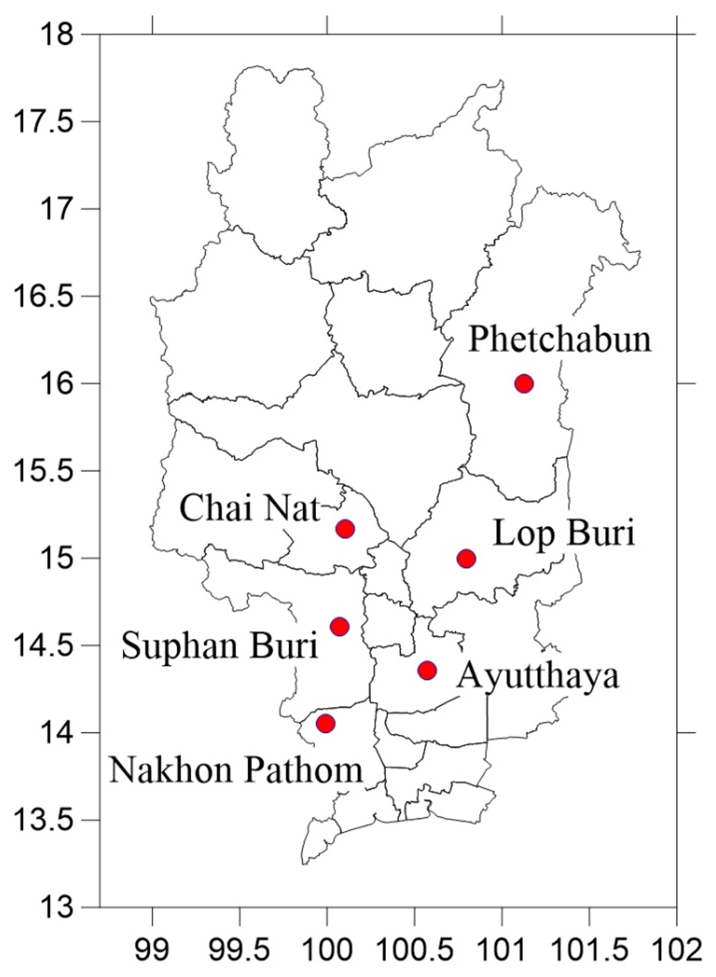
The central region is a vast plain in the center of the country. It is characterized by a large river basin consisting of mountains east and west, stretching parallel from the north. The trough is located on the northern highlands, down to the south at the edge of the track. Most of the area is lowland, divided into two parts: the eastern part is triangular, and the western or central regions are the rectangular area located on the bottom of the Gulf of Thailand. The central region has an area of approximately 92,795 km. The central region of Thailand is located from Longitude 98 E to 101 E and Latitude 13 N to 18 N, as shown in Figure 1. Most of the topography is lowlands, suitable for cultivation. The central population grows rice as the main occupation because the land contains infertile areas and river plains. The ground is sloped from the north and gradually slopes into the Gulf of Thailand in the south. Especially in the lower Chao Phraya River basin, it is higher than the sea level. The central region has an average temperature of 27–28 C, which is quite hot. The average precipitation of the region is about 1375 mm. Most of the area is in a confined zone, and it rains the most in September. Therefore, the central region is an important area for rice cultivation from the past to the present, especially in Nakhon Pathom, Suphan Buri, Chainat, Ayutthaya, Lopburi, and Phetchabun. Rice yield data were collected from the Agricultural Information Center, Office of Agricultural Economics, Ministry of Agriculture, and Cooperatives. The rice cultivar studied was Suphan Buri 1 rice from 2011 to 2018. The survey of annual rice yield per hectare was collected using the crop-cutting method using stratified two-stage sampling and systematic sampling. The district was designated as a population consisting of 490 villages with two levels of sampling units, or 9.70 percent of the total sample. The district was designated as a population consisting of two sampling units with 490 villages, representing 9.70% of the total number of samples, and three households were randomly selected. Each household randomly plots a sample and two survey points using the 30-step walk technique to frame a 1-square-meter survey and to calculate the statistics of the survey data using a simple mean calculation method.
The data necessary for developing rice yield forecasting models was the daily weather data using data from the Meteorological Department, including the highest temperature (C) data, the lowest temperature (C) data, and the internal pressure data during the morning (kPa), wind speed at an altitude of 2 m (m s), precipitation data (mm d), data from the Department of Alternative Energy Development and Efficiency, and solar radiation intensity data (kJ m d) are shown in Table 1. The rice cultivar used in this study was Suphan Buri 1, about 125 cm tall, and was not sensitive to the photoperiod. The harvest time was about 120 days, the yield was about 5037.5 kg ha [29], most of which were planted in late July to early August.
2.2. Crop Model Simulation
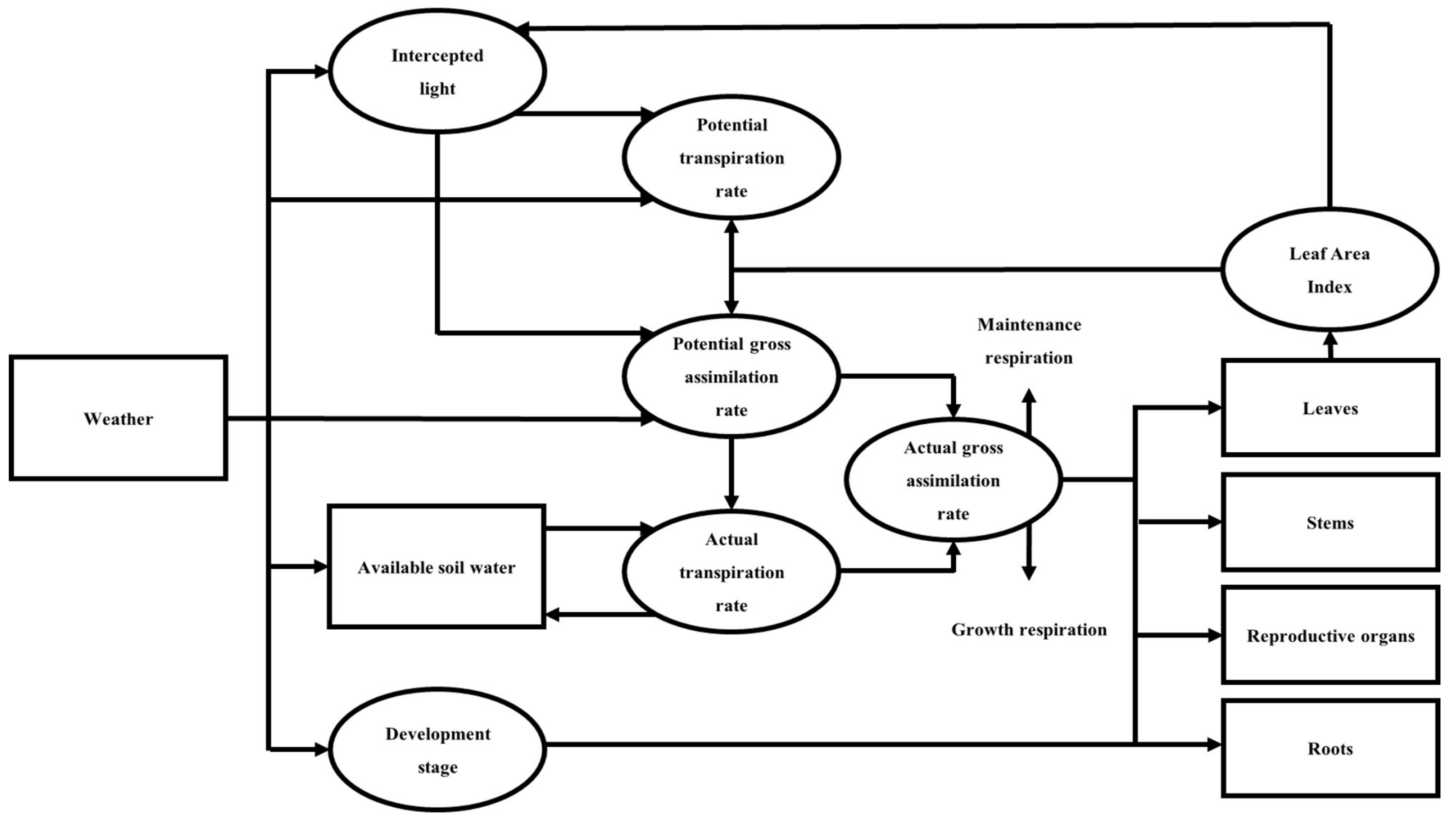
WOFOST is a mathematical model used in agriculture to study the behavior of biennial crops [30,31]. WOFOST is a daily plant growth simulation model. It is assumed that the system’s state can be quantified over time and that the changes in the system can be explained by mathematical equations [31]. In WOFOST, the dry matter is partitioned over the four parts of the plant according to fixed distribution factors, defined as a function of the development stage. Dry matter is first partitioned between shoots and roots, as shown in Equation (1). The growth rate of leaves, stems, and storage organs is simply the product of the dry matter growth rate of the shoots (Equation (2)) and the fraction allocated to these organs (Equation (3)). The model is divided into state, rate, and driving variables. State variables are quantities such as biomass or soil water content. The driving variables characterize the influence of external factors on the system but are not influenced by internal processes such as macro-meteorological variables, radiation, air temperature, and precipitation. The rate part can be calculated from the state and driving variables [31]. The general characteristics of plant growth are modeled based on physiological ecological processes. Important processes include phenological development, light-blocking, absorption of CO, evaporation, respiration, division of absorption to organs, and formation of dry matter, as shown in Figure 2. Potential growth and water restriction are modeled dynamically daily, considering the soil characteristics and limited water production. WOFOST is based on the SUCROS (Simple and Universal Crop growth Simulator) model [32,33]. SUCROS is a plant growth model that is influenced by environmental conditions and water constraints. The concept for calculation is the rate of CO (photosynthesis) absorption of canopy plants. Limited nutrient production is calculated according to the principles of the QUEFTS (QUantitative Evaluation of the Fertility of Tropical Soils) model [34]. The QUEFTS model provides yield predictions based on two factors: fertilizer inputs and soil parameters [34,35].
The plant growth simulation in WOFOST is divided into four parts (leaves, stems, fruits, and roots) in dry matter, defined in the development process, as shown in Figure 2. In practice, this method makes it easy to partition the experimental plantings and requires accurate descriptions of the plant’s phenotypic development and cultivation period. Improper crop phenotypes or the wrong cropping period can easily make the leaf area index very high or very low. The disadvantage of static partitioning is that it does not consider the absorption processing capacity from different parts of the plant and does not take into account the environmental impact of the division. The simulation is divided between shoots and roots first as follows:
where is the dry matter growth rate of the total crop (kg ha d), is the dry matter growth rate of tyhe roots (kg ha d), is the dry matter growth rate of the shoots (kg ha d), and is the partitioning factor of the roots (kg kg). The growth rates of the leaves, stems, and storage organs are only a product of the dry matter growth rate of the shoots and the portion allocated to these organs.
where is the dry matter growth rate of an organ i (kg ha d); is the division factor of an organ i (kg kg); i is the leaves (lv), storage organs (so), or stems (st). The division factors, , is a function of the developmental stage and specific to each plant. The model is described using linear interpolation in a one-dimensional array with a developmental step as independent variables. The development stage requires that the relationship in Equation (4) must be correct; otherwise, the simulation will stop.
The total CO absorption rate is equal the amount of plant structural components produced plus the amount used for maintenance and respiration, shown in Equation (5).
where is the daily rate of absorption of CHO (kg ha d), is the rate of maintenance respiration (kg ha d), and is the respiration rate in plant growth (kg ha d). The rate of respiration to live must not exceed the total absorption rate; however, if the daily CHO absorption rate comes close to zero, this may occur, and therefore, the simulation should be stopped.
In the model, a yield mortality of 0 for the root and stem growth of plants per unit area can be easily defined as the growth rate minus the mortality, as in Equation (6). Mortality is unique to each plant and is defined as the amount of daily living biomass no longer involved in the plant process. Stem and root mortality at the developmental stage was described using linear interpolation in one-dimensional arrays with the development stage as independent variables. The rate of leaf mortality is more complex, where leaf degradation due to obscured by light should consider water and physiological age. The growth rate of stems and roots can be explained by
where is the net dry matter growth rate of organ i (kg ha d), is the dry matter growth rate of organ i (kg ha d), is the dry matter weight of organ i (kg kg), is the death rate of organ i (kg ha d), and i is stems (st) or roots (rt). Stem and root mortality is a characteristic feature of the crop. Although the process describing leaf mortality is more complex than calculating stem and root mortality, calculating the total weight of live leaves is similar to calculating the stem and root weights. The total weight of the living plant (leaves, stems, and roots) can be obtained by combining them during the actual plant growth period.
where is the dry matter weight of organ i at time step t (kg ha) and is the time step (d). In the model, the default values for each plant weight are calculated. The default values for the plant weight must be specified and can be derived from planting density and seed weight. This value is multiplied by the partitioning factors, , at emergence, yielding the initial values of dry weight of the various organs.
2.3. The El Niño–Southern Oscillation
El Niño is a phenomenon in which the atmospheric pressure at sea level in the eastern Pacific Ocean is lower than usual, while the other side of the ocean pressure (Indonesia and northern Australia) is higher than usual. It connects and occurs along with the weak south–east wind until it becomes a western wind. It blows the sea from the west Pacific Ocean to the central and eastern Pacific Ocean. Scientists often use the terms ENSO warming (ENSO warm event or warm phase of ENSO) to describe an El Niño phenomenon in which the SST in the central and eastern Pacific are warmer than normal. La Niña is an abnormally cold ocean temperature phenomenon (ENSO cold event or cold phase of ENSO). It describes the phenomenon in which the SST in the central and eastern Pacific are cooler than normal. A La Niña phenomenon first appeared in early 2011 [37].
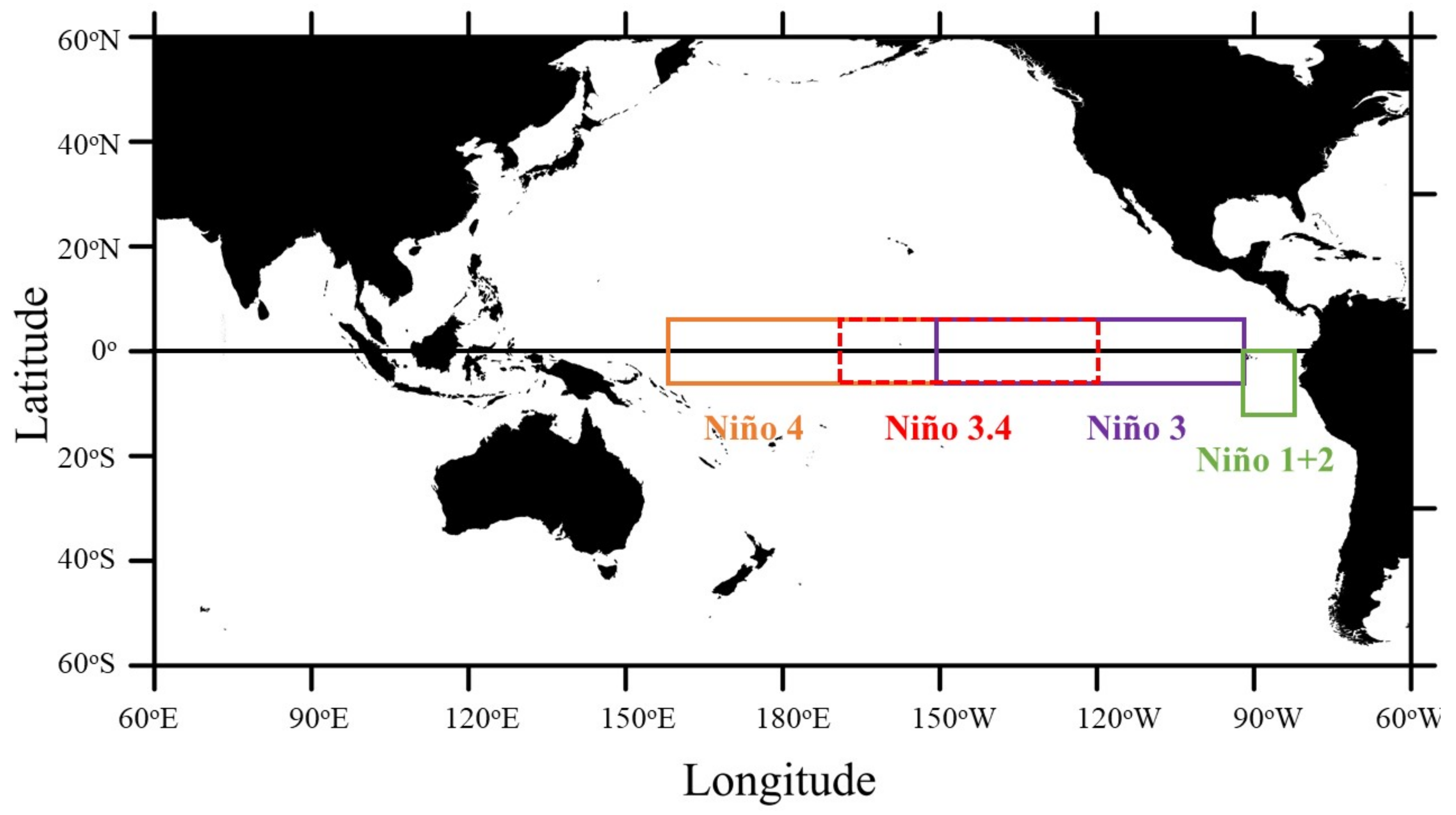
A Niño 3.4 region (5 N–5 S, 120 W–170 W) is the standard region used by the National Oceanic and Atmospheric Administration (NOAA) to identify El Niño (warm) and La Niño (cold) in the tropical Pacific Ocean as shown in Figure 3. The event is defined as having three months with a higher than +0.5 anomaly for warm events (El Niño) and with an anomaly at or below −0.5 for cold events (La Niña). The criteria are divided into additional weakness (with irregularities 0.5 to 0.9 SST), moderate (1.0 to 1.4), strong (1.5 to 1.9), and very severe events (≥2.0).
2.4. The Evaluation of the Model
The evaluation of the model was performed by collecting historical rice yield data, analyzing the growth characteristics of rice, and selecting rice strains. The selection method was based on economic importance, such as the number of productions, product prices, and historical export amount from the Office of Agricultural Economics. To compare the rice yields obtained from the model, the Root Mean Square Error (RMSE) expressed as Equation (8) and the Absolute Percent error (APE) in Equation (9) were used to evaluate the model results and to find the rice parameters suitable for cultivation. To evaluate whether the model’s trend is overestimated or underestimated, the Coefficient of Residual Mass (CRM) was used, as expressed in Equation (10). Positive values for CRM indicate that the measure is underestimated, and negative values for CRM indicate a tendency to overestimate: minimum = , maximum = +∞, while optimal is 0.
where is the Suphan Buri 1 rice yield data from the WOFOST model at time t, is the Suphan Buri 1 rice yield data from the measured data from the Department of Agricultural Statistics at time t, t is the time, and n is the total time.
The estimation of crop yield under extreme climate events (El Niño and La Niña events) was not included in the WOFOST model. Therefore, this study attempted to find the relationship between the weather conditions in the central region of Thailand and ENSO phenomena. Precipitation forecasts from ENSO phenomena were made by constructing multiple linear regression (MLR) equations. The independent variable of MLR is the average 30-year precipitation data from 1981 to 2010 (), and the SST anomaly index in the Niño 3.4 area (). The dependent variable is the precipitation data for each province (Y), as shown in Equation (11).
where Y is the precipitation data for each province; is the average 30-year precipitation data from 1981 to 2010; is the SST anomaly index in the Niño 3.4 area; and A, B, and C are constant coefficients.
3. Results
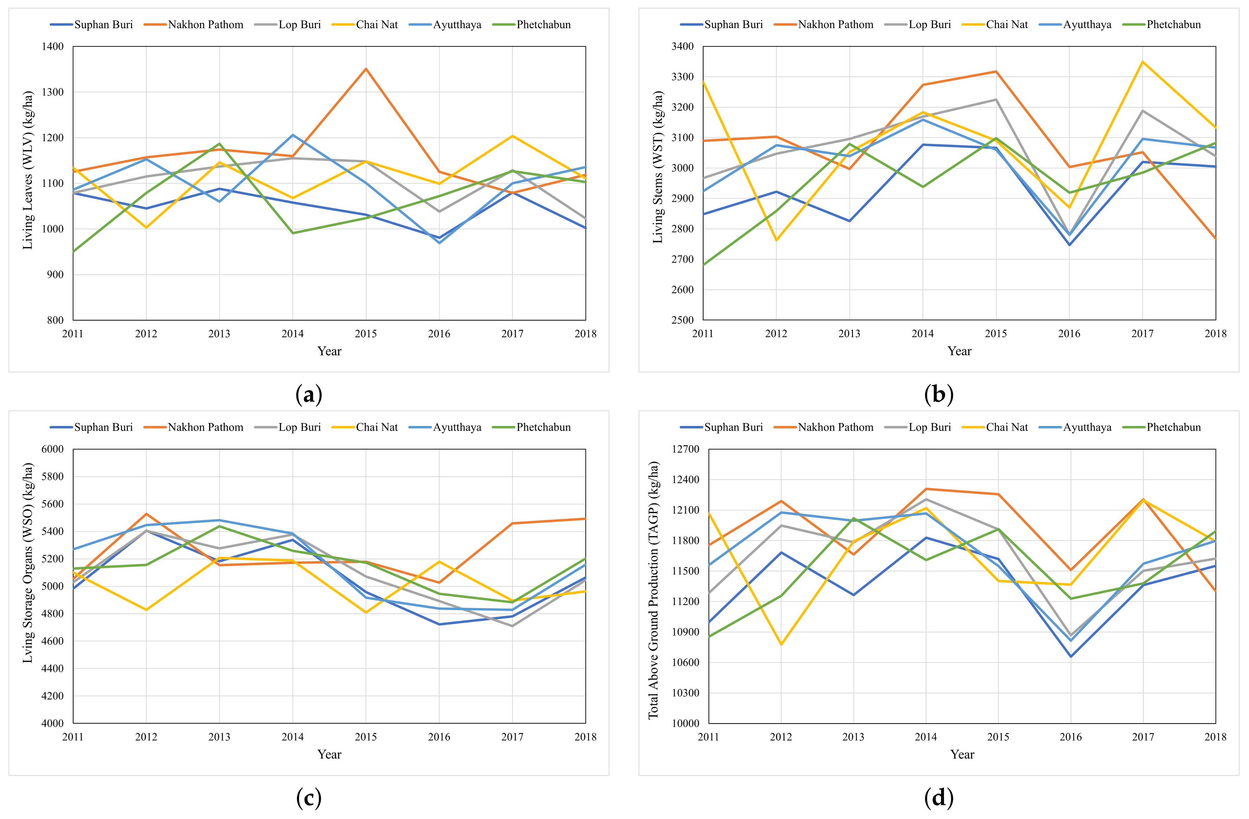
In this study, the simulation of rice yield was conducted using the WOFOST model, which models the growth and yield of a crop in the absence of injuries. The parameters of the WOFOST model were re-calibrated using the data in Thailand. The methodological framework of this study includes two procedures. The results of the WOFOST model are compared with the survey data from the Department of Agricultural Statistics, first, to verify that the model’s algorithms work properly and, second, to find the relationship between the Suphan rice yield and ENSO phenomena to determine the effect of rice yield. Model assessments were performed using historical data covering 2011 to 2018. The simulation results were compared with the observed data using statistical methods to determine whether WOFOST could simulate the growth of Suphan Buri 1 rice. Figure 4 shows the dry weight of living leaves (WLV), dry weight of living stems (WST), dry weight of living storage organs (WSO), and total above-ground production (dead and living plant organs) (TAGP) using the WOFOST model, as shown in Figure 4.
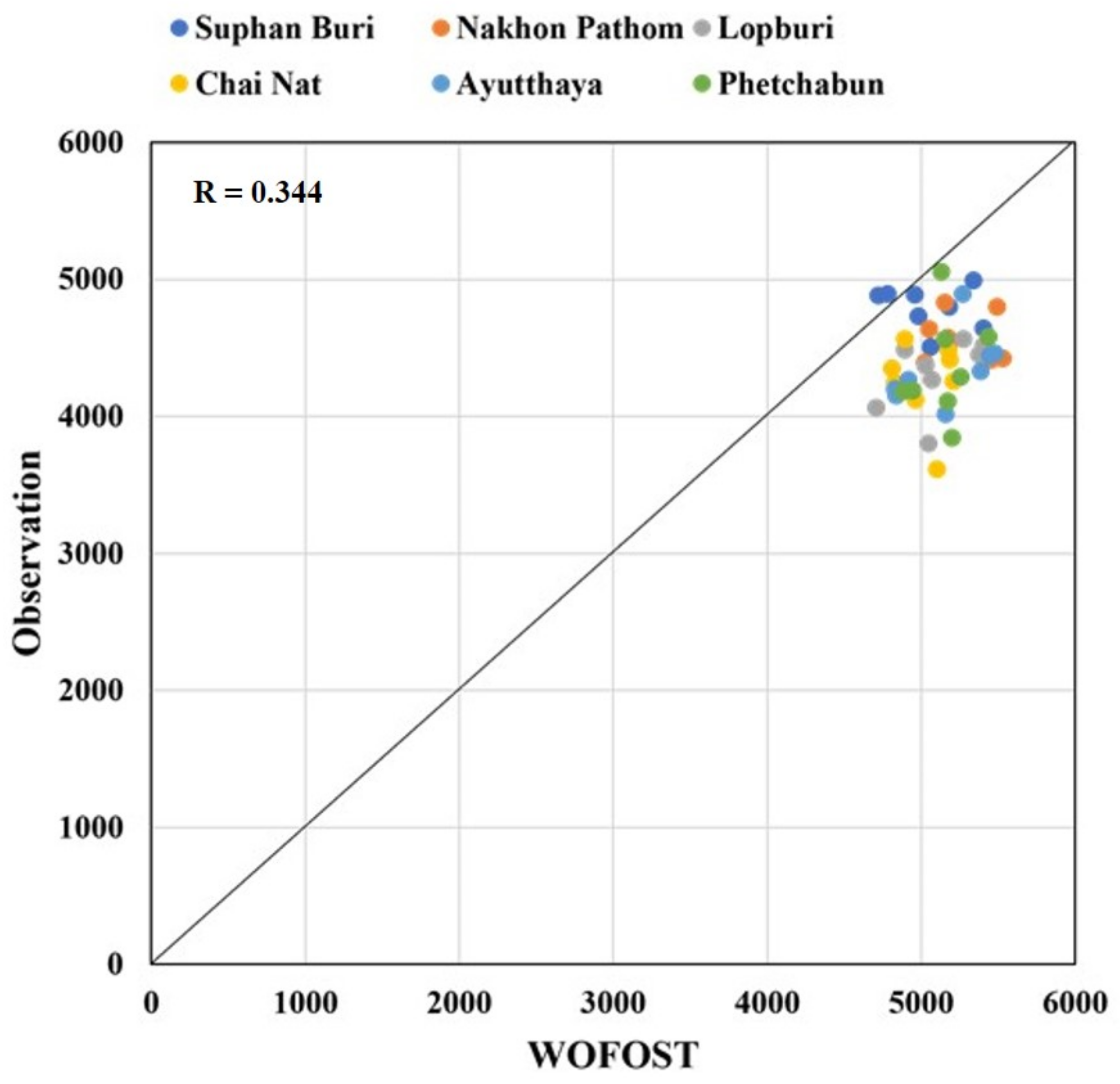
Figure 5 compares the simulated and observed rice yields of six provinces in central Thailand provinces from 2011 to 2018. Most rice yield simulations in the central region were overestimated (except Suphan Buri) because the model did not cover crop damage factors such as rice disease or insect damage. The Suphan Buri province had the closest simulation result because it used some measurement data on soil and crop management in Suphan Buri province. On the other hand, Phetchabun province had the greatest productivity difference due to its proximity to the northeastern region, where the soil characteristics were sandy. The soil in Phetchabun is medium to gravel soil and dense rubble. The topsoil is sandy loam, which is not suitable for planting. In Figure 6, the correlation coefficient for all six provinces is 0.344, which shows that the model has a low correlation. Due to some model’s input data, the data are not yet available. Therefore, soil data and plant growth data from nearby rice varieties were substituted, which may cause discrepancies in rice yields.
In order to assess the accuracy of the model, visual comparisons are, of course, not sufficient, so further tests are performed with statistical parameters such as RMSE, APE, and CRM. From the comparison, it was found that Suphan Buri province had less errors than other provinces in the central region, where the RMSE value was approximately 397.117 kg ha, which had an error of approximately 6.9%. Ratchaburi province has a greater error than other provinces in the central region, with an RMSE value of about 870.754 kg ha with an error of about 18.9%. From simulating the yield of rice varieties Suphan Buri 1, it was found that the WOFOST model was able to simulate rice yield with an average RMSE of approximately 751.80 kg ha and an percentage error of approximately 16.2%, as shown in Table 2.
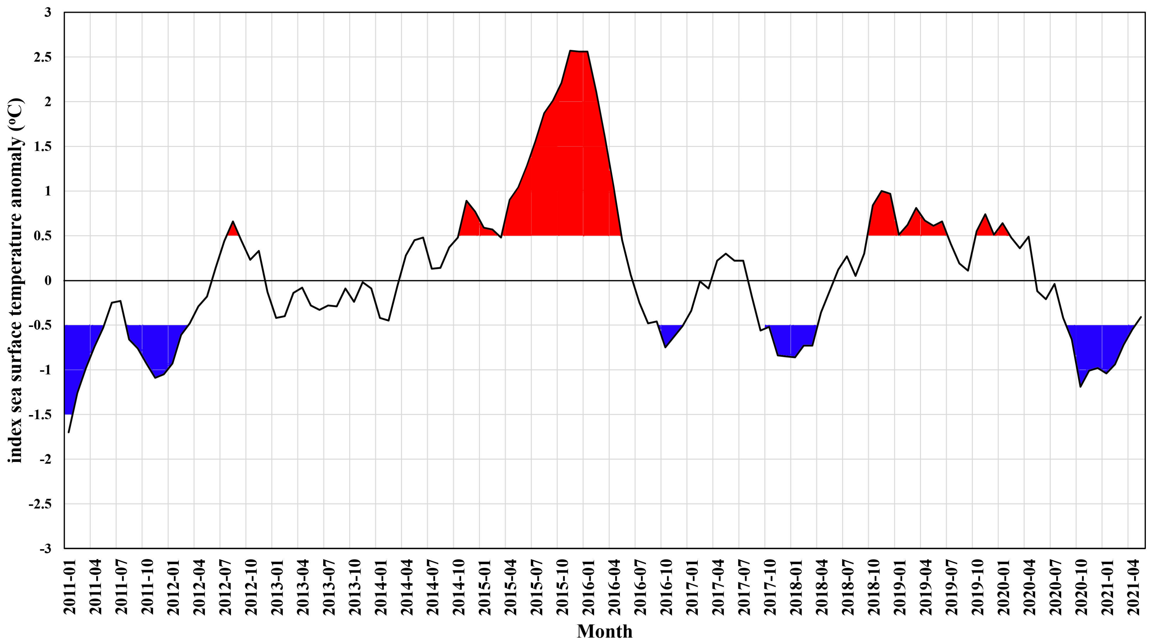
The occurrence of ENSO phenomena at Niño 3.4 from 2011 to 2018 found that, at the beginning of 2011, a severe La Niña phenomenon had been reduced to normal in April 2011, which affects Thailand as more rain than usual. From May 2015 to May 2016, a severe El Niño phenomenon occurred. From September 2017 to April 2018, there was a moderate La Niña phenomenon, and from September to December 2018, there was another moderate El Niño phenomenon, shown in Figure 7.
The correlation between Suphan Buri 1 rice variety in the central region compared with sea surface temperature anomaly at Niño 3.4 using statistical methods with the correlation coefficient is shown in Table 3. Most of the correlation coefficients were negative from statistical testing, indicating that Suphan Buri 1 rice yield was inversely related to ENSO phenomena. During the next 5–9 months of lag time, the p-value was between 0.0047 and 0.0413. The statistical significance level analysis revealed that the significance (two-tailed) was less than the 0.05 level of significance.
It was shown that ENSO phenomena are related to Suphan Buri 1 rice yield at a significance level of 0.05. The p-value of the eight-month Lag Time was 0.0047, which was less than the significance level of 0.01, indicating that ENSO phenomena are related to Suphan Buri 1 rice yield at the significance level of 0.01. It shows that, when El Niño occurs in the Niño 3.4 area, it causes less precipitation in central Thailand. El Niño phenomena affected the growth of Suphan Buri 1 rice, causing the rice yield in the next eight months to be lower than usual. On the other hand, when an La Niña phenomenon occurs in Niño 3.4, it causes more precipitation in central Thailand than usual. This affects the growth of Suphan Buri 1 rice, resulting in higher yields within the next eight months than usual.
A comparison of precipitation data from multivariate linear regression with precipitation data from measurement stations of the Meteorological Department in each province from January 2011 to December 2020 (10 years) is shown in Table 2. It was found that precipitation from the linear regression equation was related to the average precipitation data in each province. The correlation coefficient (R) equals 0.775, and the coefficient of determination (R) value was 0.601. From statistical testing, it was found that the precipitation forecasts from linear regression equations were accurate.
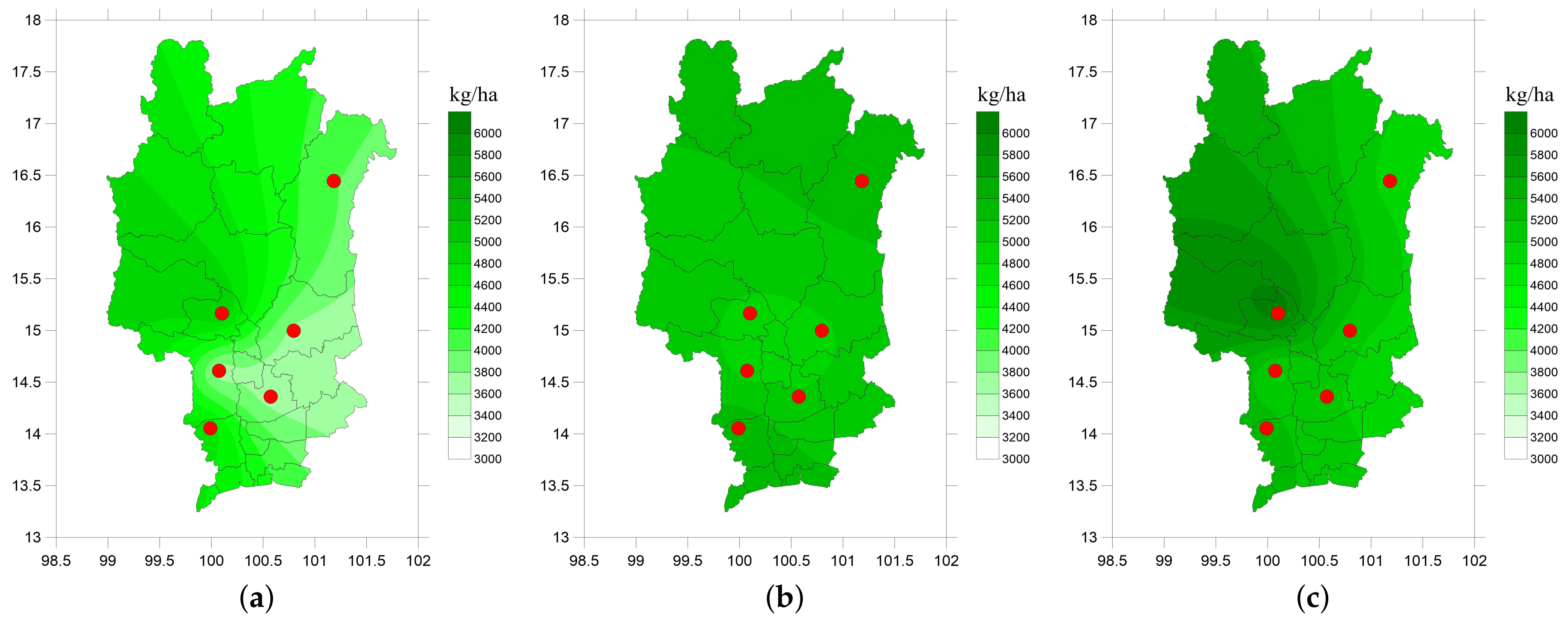
The seasonal rice yield of each province in central Thailand was estimated for the 2019–2021 period based on ENSO phenomena, as shown in Figure 8. The escalating threat of an ENSO anomaly affects climate change, coupled with future losses to rice production from droughts (El Niño) and floods (La Niña). Accordingly, the climate change scenarios from ENSO phenomena affect rice yield in Thailand. The mapping delineates the consequences of El Niño and La Niña events with future impacts on rice production. Interestingly, during El Niño years (2019), simulated rice yields were lower at about 4300 kg per hectare than in other years. This is because the extremely unfavorable conditions for rice growth (drought) result in fewer rice yields than usual. The rice yields in 2020 were normal as a result of no ENSO phenomena occurring in that year. Furthermore, the rice yields in 2021 were higher than other years at about 5200 kg per hectare because there was a La Niña effect that year. A La Niña event strengthening rice yield can be explained by the increased precipitation in Thailand, which is sufficient to support the need for water for rice growth. The variation in rice yields shows the significant impact from El Niño and La Niña events in Thailand.
4. Conclusions and Discussion
The simulation of rice yield was performed using the WOFOST model, which models the growth and yield of a crop in the absence of injuries. The parameters of the WOFOST model were re-calibrated using the data in Thailand. The rice cultivar studied was Suphan Buri 1 from 2011 to 2018. The study areas are six provinces in the central region of Thailand, an important area for rice cultivation from the past to the present, especially in the provinces of Nakhon Pathom, Suphan Buri, Chainat, Ayutthaya, Lopburi, and Phetchabun. The methodological framework of this study includes two procedures. The results of the WOFOST model are compared with survey data from the Department of Agricultural Statistics, first, to verify the model’s algorithms are working properly and, second, to find the relationship between Suphan rice yield and ENSO phenomena to determine the effect of rice yield. The rice yield simulations in the central region were overestimated (except Suphan Buri) because the model did not cover crop damage factors such as rice disease or insect damage. Suphan Buri province had the closest simulation result because it used some measurement data on soil and crop management in Suphan Buri province. The results were analyzed using the RMSE, APE, and CRM statistics. The WOFOST model yielded RMSE values for all six provinces at 752 kg ha, with approximately 16% error and a CRM value of . On the province scale, the WOFOST model was able to simulate the actual rice yield.
ENSO is associated with abnormal climatic conditions such as temperature and precipitation across the globe. As a result, Thailand is experiencing drought and water shortages in agriculture. Therefore, an attempt was made to find the relationship between ENSO phenomena and rice yield. The correlation between rice yields from the six provinces in the central part of Thailand using the WOFOST model and ENSO phenomena in Niño 3.4 showed that the correlation coefficient was approximately −0.4, with a delay of 8 months. It shows that, when an El Niño phenomenon occurs at Niño 3.4, it results in lower-than-normal yields of Suphan Buri 1 rice in the next 8 months. In El Niño years, rice yield decreased around 8.5% in 2019. On the other hand, when a La Niña phenomenon occurs at Niño 3.4, Suphan Buri 1 rice yields are higher than normal in the next 8 months. La Niña years lead to increased precipitation in Thailand, e.g., rice yield increased by around 12.7% in 2021. The analysis of rice yield data confirms the significant impact of ENSO on rice yields in Thailand. This study shows that climate change leads to impacts on rice production, especially during ENSO years. Currently, ENSO forecasts are highly accurate for short-term adaptation. Therefore, it is important to research and develop a production plan to adapt the planting system to suit El Niño or La Niña situations.
Our study also has some limitations. Restrictions on the input data from experimental plots did not cover all parameters of the WOFOST model. The rice yields from the WOFOST model were higher than rice yields measured in all provinces because the simulation did not account for death from rice disease or insect damage. Rice quality may be one of the factors that reduce market value and income. This study did not consider the impact on rice quality. Another reason is the low spatial resolution of input parameters such as meteorology, crops, management, etc. Due to the limited collection of data over a large area, the results of the WOFOST model still have some discrepancies. The climate factors of macro-meteorological variables, radiation, air temperature, and precipitation made significant contributions to the predictions of rice yield.
Author Contributions
Conceptualization, S.H. and S.I.; methodology, S.H.; software, S.I.; validation, S.H., S.I., P.V. and U.H.; formal analysis, S.H.; investigation, S.H.; resources, S.I.; data curation, S.I.; writing original draft preparation, P.V.; writing review and editing, U.H.; visualization, P.V.; supervision, U.H.; project administration, U.H.; funding acquisition, P.V. All authors have read and agreed to the published version of the manuscript.
Funding
This research was supported by the Program Management Unit for Human Resources and Institutional Development, Research, and Innovation, NXPO (grant number B16F630087) and by the Thailand Science Research and Innovation (TSRI) Basic Research Fund: Fiscal year 2022.
Conflicts of Interest
The authors declare no conflict of interest.
Abbreviations
The following abbreviations are used in this manuscript:
| APE | Absolute Percent Error |
| CRM | Coefficient of Residual Mass |
| ENSO | El Niño and Southern Oscillation |
| QUEFTS | Quantitative Evaluation of the Fertility of Tropical Soils |
| R | Correlation Coefficient |
| R | Coefficient of Determination |
| RMSE | Root Mean Square Error |
| SUCROS | Simple and Universal Crop growth Simulator |
| TAGP | Total Above-Ground Production |
| WOFOST | World Food Studies |
| WSO | Living Storage Organs |
| WST | Living Stems |
| WLV | Living Leaves |
References
- Zibaee, A. Rice: Importance and Future. Rice Res. 2013, 1, 1. [Google Scholar] [CrossRef] [Green Version]
- Gnanamanickam, S.S. Biological Control of Rice Diseases. Biol. Control Rice Dis. 2009, 8, 1–11. [Google Scholar]
- Zeigler, R.S.; Barclay, A. The Relevance of Rice. Rice 2008, 1, 3–10. [Google Scholar] [CrossRef] [Green Version]
- Sander, J.C.J.; Cheryl, H.P.; Andrew, D.M.; Ioannis, N.A.; Ian, F.; James, W.J.; John, M.A. Towards a new generation of agricultural system data, models and knowledge products: Information and communication technology. Agric. Syst. 2017, 155, 200–212. [Google Scholar]
- Verónica, S.R.; Francisco, R.M. From Smart Farming towards Agriculture 5.0: A Review on Crop Data Management. Agronomy 2020, 10, 207. [Google Scholar]
- Fermont, A.; Todd, B. Estimating Yield of Food Crops Grown by Smallholder Farmers: A Review in the Uganda Context. Int. Food Policy Res. Inst. 2011, 1, 68. [Google Scholar]
- Mukherjee, J.; Singh, L.; Singh, G.; Bal, S.K.; Singh, H.; Kaur, P. Comparative Evaluation of WOFOST and ORYZA2000 Models in Simulating Growth and Development of Rice (Oryza Sativa L.) in Punjab. J. Agrometeorol. 2011, 13, 86–91. [Google Scholar]
- Koide, N.; Robertson, A.W.; Ines, A.V.M.; Qian, J.H.; DeWitt, D.G.; Lucero, A. Prediction of Rice Production in the Philippines Using Seasonal Climate Forecasts. J. Appl. Meteorol. Climatol. 2013, 52, 552–569. [Google Scholar] [CrossRef] [Green Version]
- Putri, R.E.; Yahya, A.; Adam, N.M.; Aziz, S.A. Rice yield prediction model with respect to crop healthiness and soil fertility. Food Res. 2019, 3, 174–180. [Google Scholar]
- Vijayalata, V.; Devi, V.N.R.; Rohit, P.; Kiran, G.S.S.R. A Suggestive Model for Rice Yield Prediction and Ideal Meteorological Conditions During Crisis. Int. J. Sci. Technol. Res. 2019, 8, 1572–1576. [Google Scholar]
- Mardianto, M.; Tjahjono, E.; Rifada, M. Statistical modelling for prediction of rice production in indonesia using semiparametric regression based on three forms of Fourier series estimator. J. Eng. Appl. Sci. 2019, 14, 2763–2770. [Google Scholar]
- Guo, Y.; Xiang, H.; Li, Z.; Ma, F.; Du, C. Prediction of Rice Yield in East China Based on Climate and Agronomic Traits Data Using Artificial Neural Networks and Partial Least Squares Regression. Agronomy 2021, 11, 282. [Google Scholar] [CrossRef]
- Jin, M.; Liu, X.; Wu, L.; Liu, M. An improved assimilation method with stress factors incorporated in the WOFOST model for the efficient assessment of heavy metal stress levels in rice. Int. J. Appl. Earth Obs. Geoinf. 2015, 41, 118–129. [Google Scholar] [CrossRef]
- Eitzinger, J.; Trnka, M.; Hösch, J.; Žalud, Z.; Dubrovský, M. Comparison of CERES, WOFOST and SWAP models in simulating soil water content during growing season under different soil conditions. Ecol. Model. 2004, 171, 223–246. [Google Scholar] [CrossRef]
- Todorovic, M.; Albrizio, R.; Zivotic, L.; Saab, M.T.A.; Stöckle, C.; Steduto, P. Assessment of AquaCrop, CropSyst, and WOFOST models in the simulation of sunflower growth under different water regimes. Agronomy 2009, 101, 509–521. [Google Scholar] [CrossRef]
- Ma, Y.; Wang, S.; Zhang, L. Study on improvement of WOFOST against overwinter of wheat in North China. Chin. J. Agrometeorol. 2005, 26, 145–149. [Google Scholar]
- Supit, I.; Hooijper, A.A.; Diepen, V.C.A. System Description of WOFOST6.0 Crop Simulation Model Implemented in CGMS, Theory and Algorithms; Publications Office of the European Union: Luxembourg, 1994; pp. 1–144. [Google Scholar]
- Xie, W.X.; Yan, L.; Wang, G. Simulation and Validation of Rice Potential Growth Process in Zhejiang by Utilizing WOFOST Model. Zhongguo Shuidao Kexue 2006, 20, 319–323. [Google Scholar]
- Wu, D.; Ou, Y.; Zhao, X. The applicability research of WOFOST model in North China plain. Acta Phytoecol. Sin. 2003, 27, 594–602. [Google Scholar]
- Ma, S.; Pei, Z.; He, Y. Study on Simulation of Rice Yield with WOFOST in Heilongjiang Province. In Proceedings of the International Conference on Computer and Computing Technologies in Agriculture, Dongying, China, 19–21 October 2016. [Google Scholar]
- Biswas, R.; Banerjee, B.; Bhattacharyya, B. Impact of Temperature Increase on Performance of Kharif Rice at Kalyani, West Bengal Using WOFOST Model. J. Agrometeorol. 2018, 20, 28–30. [Google Scholar]
- Ratjen, A.M.; Kage, H. Forecasting yield via reference- and scenario calculations. Comput. Electron. Agric. 2015, 114, 212–220. [Google Scholar] [CrossRef]
- Jha, R.K.; Kalita, P.K.; Cooke, R.A.; Kumar, P.; Davidson, P.C.; Jat, R. Predicting the Water Requirement for Rice Production as Affected by Projected Climate Change in Bihar, India. Water 2020, 12, 3312. [Google Scholar] [CrossRef]
- Washio, K. The Prediction of Climate Change and Rice Production in Japan. Rice Res. 2013, 2, 1–3. [Google Scholar]
- Arunrat, N.; Pumijumnong, N. The Preliminary Study of Climate Change Impact on Rice Production and Economic in Thailand. Asian Soc. Sci. 2015, 11, 275–294. [Google Scholar] [CrossRef] [Green Version]
- Amnuaylojaroen, T.; Chanvichit, P.; Janta, R.; Surapipith, V. Projection of Rice and Maize Productions in Northern Thailand under Climate Change Scenario RCP8.5. Agriculture 2021, 11, 23. [Google Scholar] [CrossRef]
- TMD, Thai Meteorological Department, ENSO Phenomenon. Available online: https://www.tmd.go.th/info/info.php?FileID=19 (accessed on 10 October 2020).
- Jumpol, H. National Science and Technology Development Agency. Available online: http://nstda.or.th/rural/public/100%20articles-stkc/9.pdf (accessed on 10 February 2019).
- Rice Department. Suphan Buri 1. Available online: https://www.ricethailand.go.th/Rkb/varieties/index.php-file=content.php&id=76.htm (accessed on 4 December 2020).
- Rabbinge, R.; Wit, C.T. Systems, models and simulation. In Simulation and Systems Management in Crop Protection; Pudoc: Wageningen, The Netherlands, 1989; pp. 3–5. [Google Scholar]
- Wit, C.T. Philosophy and terminology. In On Systems Analysis and Simulation of Ecological Processes with Examples in CSMP and FORTRAN; Springer: Dordrecht, The Netherlands, 1993; pp. 3–9. [Google Scholar]
- Spitters, C.J.T.; Keulen, V.H.; Kraalingen, V.D.W.G. A simple and universal crop growth simulator: SUCROS87. In Simulation and Systems Management in Crop Protection; Pudoc: Wageningen, The Netherlands, 1989; pp. 147–181. [Google Scholar]
- Laar, V.H.H.; Goudriaan, J.; Keulen, V.H. Simulation of Crop Growth for Potential and Water-Limited Production Situations (As Applied to Spring Wheat); CABO-DLO, WAU-TPE: Wageningen, The Netherlands, 1992; pp. 1–72. [Google Scholar]
- Janssen, B.H.; Guiking, F.C.T.; Eijk, V.D.D.; Smaling, E.M.A.; Wolf, J.; Reuler, V.H. A system for quantitative evaluation of the fertility of tropical soils (QUEFTS). Geoderma 1990, 46, 299–318. [Google Scholar] [CrossRef] [Green Version]
- Smaling, E.M.A.; Janssen, B.H. Calibration of quefts, a model predicting nutrient uptake and yields from chemical soil fertility indices. Geoderma 1993, 59, 21–44. [Google Scholar] [CrossRef]
- Kropff, M.J.; Laar, V.H.H. Modeling Crop-Weed Interactions; International Rice Research Institute: Los Baños, Philippines, 1993; pp. 1–274. [Google Scholar]
- Gao, C.; Zhang, R.H. The roles of atmospheric wind and entrained water temperature (Te) in the second-year cooling of the 2010–12 La Niña event. Clim. Dyn. 2017, 48, 597–617. [Google Scholar] [CrossRef] [Green Version]
Figure 1.
Map showing rice cultivation of Suphan Buri 1 in all six provinces in the central region.

Figure 2.
General simple structure of a dynamic plant growth model [36].
Figure 2.
General simple structure of a dynamic plant growth model [36].

Figure 3.
Niño area.

Figure 4.
The results of simulating the weight of rice variety Suphan Buri. (a) WLV, (b) WST, (c) WSO, and (d) TAGP.
Figure 4.
The results of simulating the weight of rice variety Suphan Buri. (a) WLV, (b) WST, (c) WSO, and (d) TAGP.

Figure 5.
Comparison of rice yield between the WOFOST model and observed data. (a) Suphan Buri, (b) Nakhon Pathom, (c) Lop Buri, (d) Chai Nat, (e) Ayutthaya, and (f) Phetchabun.
Figure 5.
Comparison of rice yield between the WOFOST model and observed data. (a) Suphan Buri, (b) Nakhon Pathom, (c) Lop Buri, (d) Chai Nat, (e) Ayutthaya, and (f) Phetchabun.
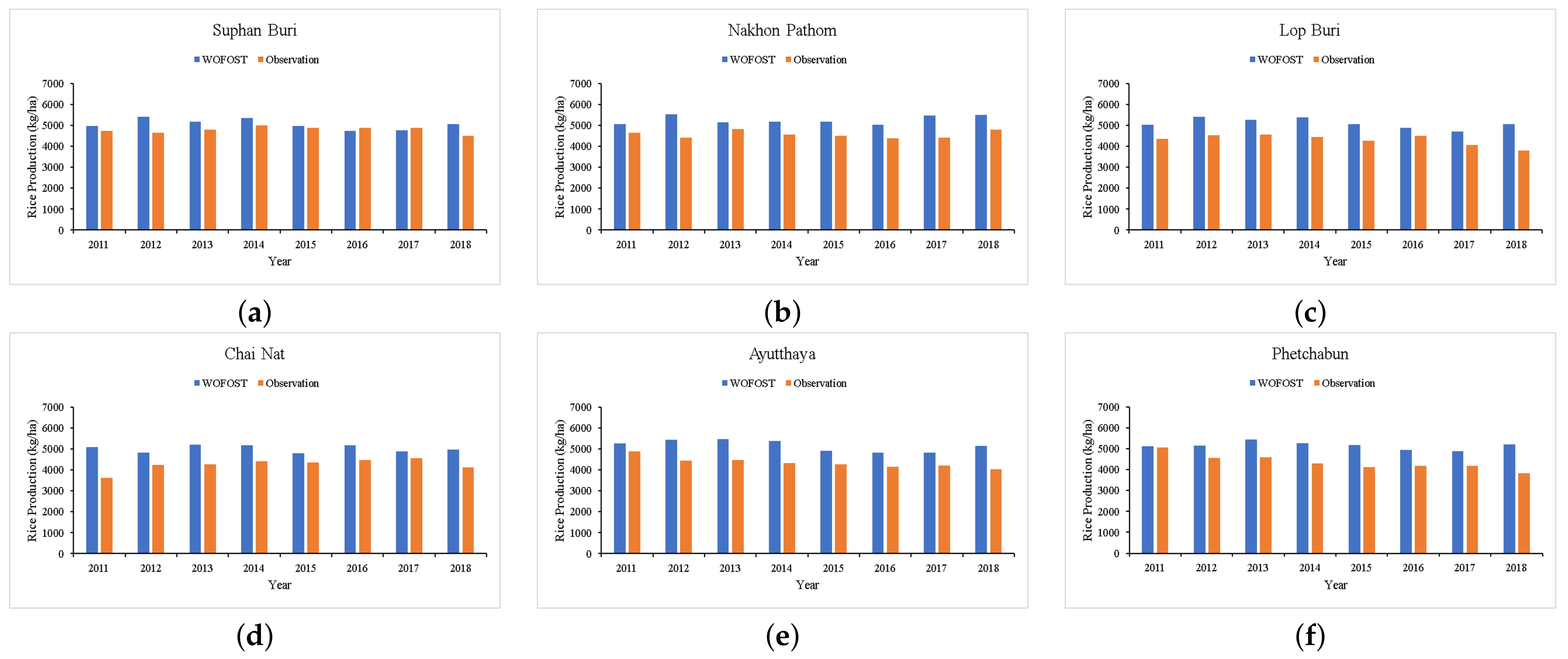
Figure 6.
Correlation of the rice yield from the WOFOST.

Figure 7.
The occurrence of ENSO phenomena at Niño 3.4 (5 S–5 N, 170 W–120 W) regions from 2011 to 2018.
Figure 7.
The occurrence of ENSO phenomena at Niño 3.4 (5 S–5 N, 170 W–120 W) regions from 2011 to 2018.

Figure 8.
Forecasted results of rice yields in the central region in 2019 to 2021: (a) 2019, (b) 2020, and (c) 2021.
Figure 8.
Forecasted results of rice yields in the central region in 2019 to 2021: (a) 2019, (b) 2020, and (c) 2021.


Table 1.
Meteorological parameters of the WOFOST model.
| No. | Describe | Unit | Year | Source |
|---|---|---|---|---|
| 1 | Maximum Air Temperature | C | 2011–2018 | Thailand Meteorological Department |
| 2 | Minimum Air Temperature | C | 2011–2018 | Thailand Meteorological Department |
| 3 | Early Morning Vapor Pressure | kPa | 2011–2018 | Thailand Meteorological Department |
| 4 | Mean Wind Speed at 2 m Above Ground | m s | 2011–2018 | Thailand Meteorological Department |
| 5 | Precipitation | mm d | 2011–2018 | Thailand Meteorological Department |
| 6 | Irradiation | kJ m d | 2011–2018 | Department of Alternative Energy |
| Development and Efficiency |
Table 2.
Accuracy comparison between the WOFOST model and observed data.
| Station | Root Mean | Absolute Percent | Coefficient of | C | A | B | R | R |
|---|---|---|---|---|---|---|---|---|
| Square Error | Error | Residual Mass | ||||||
| Suphan Buri | 397.117 | 6.991 | −0.055 | 0.282 | 0.028 | −0.183 | 0.750 | 0.563 |
| Nakhon Pathom | 731.626 | 15.150 | −0.150 | 0.266 | 0.030 | −0.348 | 0.770 | 0.592 |
| Lop Buri | 818.764 | 18.457 | −0.182 | 0.073 | 0.031 | −0.172 | 0.818 | 0.669 |
| Chai Nat | 835.593 | 18.605 | −0.180 | 0.253 | 0.029 | −0.066 | 0.747 | 0.558 |
| Ayutthaya | 856.984 | 19.049 | −0.188 | 0.588 | 0.026 | −0.365 | 0.764 | 0.583 |
| Phetchabun | 870.754 | 18.971 | −0.183 | 0.067 | 0.034 | −0.506 | 0.800 | 0.640 |
| Mean | 751.806 | 16.204 | −0.156 | − | − | − | 0.775 | 0.601 |
Table 3.
Correlation coefficient between WOFOST and ENSO phenomena.
| Lag Time | Suphan Buri | Nakhon Pathom | Lopburi | Chai Nat | Ayutthaya | Phetchabun | Sum | p-Value |
|---|---|---|---|---|---|---|---|---|
| No Lag | 0.2474 | 0.2230 | 0.2731 | −0.5442 | −0.0704 | 0.3114 | 0.0816 | 0.5812 |
| Lag 1 | 0.2767 | 0.1251 | 0.3466 | −0.5343 | −0.0397 | 0.3170 | 0.0930 | 0.5297 |
| Lag 2 | 0.2227 | 0.2337 | 0.2538 | −0.7019 | −0.1245 | 0.1435 | 0.0259 | 0.8611 |
| Lag 3 | 0.0445 | 0.2632 | 0.0399 | −0.7803 | −0.2988 | −0.0203 | −0.1001 | 0.4983 |
| Lag 4 | −0.0490 | 0.0529 | −0.0100 | −0.5561 | −0.4174 | −0.1154 | −0.1631 | 0.2680 |
| Lag 5 | −0.3050 | −0.1462 | −0.2058 | −0.2770 | −0.6184 | −0.2826 | −0.2957 | 0.0413 |
| Lag 6 | −0.4505 | −0.3401 | −0.2718 | −0.0047 | −0.6448 | −0.3315 | −0.3389 | 0.0184 |
| Lag 7 | −0.5042 | −0.4449 | −0.2896 | 0.1927 | −0.5901 | −0.3704 | −0.3372 | 0.0191 |
| Lag 8 | −0.5959 | −0.3630 | −0.4019 | 0.1016 | −0.6825 | −0.4732 | −0.4016 | 0.0047 |
| Lag 9 | −0.5436 | −0.4027 | −0.3335 | 0.1778 | −0.6232 | −0.3870 | −0.3556 | 0.0131 |
Publisher’s Note: MDPI stays neutral with regard to jurisdictional claims in published maps and institutional affiliations. |
© 2021 by the authors. Licensee MDPI, Basel, Switzerland. This article is an open access article distributed under the terms and conditions of the Creative Commons Attribution (CC BY) license (https://creativecommons.org/licenses/by/4.0/).
Share and Cite
MDPI and ACS Style
Hensawang, S.; Injan, S.; Varnakovida, P.; Humphries, U. Predicting Rice Production in Central Thailand Using the WOFOST Model with ENSO Impact. Math. Comput. Appl. 2021, 26, 72. https://doi.org/10.3390/mca26040072
AMA Style
Hensawang S, Injan S, Varnakovida P, Humphries U. Predicting Rice Production in Central Thailand Using the WOFOST Model with ENSO Impact. Mathematical and Computational Applications. 2021; 26(4):72. https://doi.org/10.3390/mca26040072
Chicago/Turabian StyleHensawang, Saruda, Sittisak Injan, Pariwate Varnakovida, and Usa Humphries. 2021. "Predicting Rice Production in Central Thailand Using the WOFOST Model with ENSO Impact" Mathematical and Computational Applications 26, no. 4: 72. https://doi.org/10.3390/mca26040072