Numerical and Theoretical Stability Study of a Viscoelastic Plate Equation with Nonlinear Frictional Damping Term and a Logarithmic Source Term

Abstract

This paper is designed to explore the asymptotic behaviour of a two dimensional visco-elastic plate equation with a logarithmic nonlinearity under the influence of nonlinear frictional damping. Assuming that relaxation function g satisfies $g^{\prime }\left(t\right)\le -\xi \left(t\right)\mathbb{G}\left(g\left(t\right)\right)$, we establish an explicit general decay rates without imposing a restrictive growth assumption on the damping term. This general condition allows us to recover the exponential and polynomial rates. Our results improve and extend some existing results in the literature. We preform some numerical experiments to illustrate our theoretical results.

1. Introduction

Denote $\mathsf{\Omega }$ to be an open bounded domain of ${\mathbb{R}}^2$ having a smooth boundary $\partial \mathsf{\Omega }$. Let $n$ stands for the unit outer normal to $\partial \mathsf{\Omega }$. We then consider the following plate model:

$$\begin{array}{c}\hfill \left\{\begin{array}{c}{u}_{tt}+{\Delta }^{2}u+u-{\int }_0^{t}g(t-\tau ){\Delta }^{2}u\left(\tau \right)d\tau +h\left(u_t\right)=kuln\left|u\right|,x\in \mathsf{\Omega },t>0\hfill \\ u(x,t)=\frac{\partial u}{\partial n}(x,t)=0,x\in \partial \mathsf{\Omega },t>0\hfill \\ u(x,0)=u_0\left(x\right),u_t(x,0)=u_1\left(x\right),t>0.\hfill \end{array}\right.\end{array}$$

(1)

In this model, the parameter g is assumed to be a positive and decreasing function while k is taken to be small positive real number. After the pionnering work of Dafermos [1], many authors have continue to explore visco-elastic models with various kinds of nonlinearities and damping effects. Lagnese [2] showed that the energy decays to zero as time goes to infinity by the introduction of a dissipative mechanism on the boundary of the system. Besides, Rivera et al. [3] showed that, if the memory kernel decays exponentially as well, then both the first and second order energy related to the solutions of the viscoelastic plate equation decay exponentially. Komornik later in [4] investigated the energy decay while assuming a weak growth assumption. Furthermore, Messaoudi [5] for the following problem,

$$\begin{array}{c}\hfill \left\{\begin{array}{cc}{u}_{tt}+{\Delta }^{2}u+|u_t{|}^{m-2}{u}_t={\left|u\right|}^{p-2}u,\hfill & \mathrm{in}{Q}_T=\mathsf{\Omega }\times (0,T),\hfill \\ u=\frac{\partial u}{\partial n}=0,\hfill & \mathrm{on}{\mathsf{\Gamma }}_T=\partial \mathsf{\Omega }\times [0,T),\hfill \\ u(x,0)=u_0\left(x\right),u_t(x,0)=u_1\left(x\right),\hfill & \mathrm{in}\mathsf{\Omega },\hfill \end{array}\right.\end{array}$$

(2)

developed an existence result and further demonstrated that the solution exists globally if $m\ge p$. However, this solution blows up in finite time provided $m<p$ and the initial energy is negative. Chen and Zhou [6] later improved the result in [5]. The importance of nonlinearity cannot be overemphasized, it occurs naturally in many fields especially in nuclear physics and quantum mechanics [7,8]. In the earliest work of Birula and Mycielski [9], they considered the following problem:

$$\begin{array}{c}\hfill \left\{\begin{array}{c}{u}_{tt}-u_{xx}+u-\lambda uln{\left|u\right|}^2=0,(x,t)\in [a,b]\times (0,T),\hfill \\ u(a,t)=u(b,t)=0,t\in (0,T),\hfill \\ u(x,0)=u_0\left(x\right),u_t(x,0)=u_1\left(x\right),x\in [a,b].\hfill \end{array}\right.\end{array}$$

(3)

The authors demonstrated that in any dimensions, wave equations with this nonlinearity have localized and stable soliton-like solutions. Cazenave and Haraux in [10] established the wellposedness of the associated Cauchy problem of

$$u_{tt}-\Delta u=uln{\left|u\right|}^k,\mathrm{in}{\mathbb{R}}^3.$$

(4)

In the case of one-dimensional, Gorka [11] used some compactness results to obtain the global existence of weak solutions to the initial-boundary value problem of Equation (4). Still on logarithmic nonlinearity, Al-Gharabli and Messaoudi [12] proved the global existence and the exponential decay of solutions of the following plate equation:

$$\begin{array}{c}\hfill \left\{\begin{array}{c}{u}_{tt}+{\Delta }^{2}u+u+h\left(u_t\right)=kuln\left|u\right|,x\in \mathsf{\Omega },t>0\hfill \\ u(x,t)=\frac{\partial u}{\partial n}(x,t)=0,x\in \partial \mathsf{\Omega },t>0\hfill \\ u(x,0)=u_0\left(x\right),u_t(x,0)=u_1\left(x\right),t>0.\hfill \end{array}\right.\end{array}$$

(5)

For more recent works regarding nonlinearity, we refer [13,14,15,16,17,18,19,20,21,22,23]. For the relaxation function, Cavalcanti et al. [24], reported an exponential decay result using relaxation functions which satisfy,

$$-{\xi }_{2}g\left(t\right)\ge g^{\prime }\left(t\right)\ge -{\xi }_{1}g\left(t\right),t\ge 0.$$

In 2008, Messaoudi [25,26] generalized the decay rates permitting an extended class of relaxation functions. He considered a relaxation function that satisfy

$$-\xi \left(t\right)g\left(t\right)\ge g^{\prime }\left(t\right),t\ge 0,$$

(6)

where $\xi :{\mathbb{R}}^{+}\to {\mathbb{R}}^{+}$ is a non-increasing differentiable function. Afterwards, relaxation functions satisfying

$$-\chi \left(g\left(t\right)\right)\ge g^{\prime }\left(t\right),$$

(7)

with constraints imposed on $\chi$, have been used by several authors. Please, see [27,28,29]. Al-Gharabli et al. [30] considered the following problem:

$$u_{tt}+{\Delta }^{2}u+u-{\int }_0^{t}g(t-\tau ){\Delta }^{2}u\left(\tau \right)d\tau +h\left(u_t\right)=kuln\left|u\right|.$$

They proved an existence and decay results of the solutions under the condition that the relaxation function g satisfies

$$-\xi \left(t\right)g^p\left(t\right)\ge g^{\prime }\left(t\right),\forall t\ge 0,1\le p<\frac{3}{2}.$$

(8)

After extensive studies of the literature on wave models with logarithmic nonlinearities, especially [11,14,29,31], we seek to extend this kind of nonlinear effects to a plate equation. However, we consider general dampings unlike the ones considered in [12,29,30]. It is worth to mention that even-though the logarithmic nonlinearities are not as strong as the polynomial nonlinearities, the method used for establishing the existence and stability results in the case of polynomial nonlinearities cannot be directly adopted. The remaining part of this introduction section contains some basic notations and preliminary results required for this work. Section 2 presents the global and local existence of the solutions to the problem. Our technical Lemmas and decay results are in Section 3 and Section 4. Finally, Section 5 contains the numerical results.

Preliminaries

We denote $L^2\left(\mathsf{\Omega }\right)$ and $H_0^2\left(\mathsf{\Omega }\right)$ as the usual Lebesgue and Sobolev spaces respectively equipped with their usual scalar products and norms. Throughout this paper, unless specified, c represents a generic constant. The following assumptions are important for this work:

$\left(\mathbb{A}1\right)$

$g:{\mathbb{R}}^{+}\to {\mathbb{R}}^{+}$ is a $C^1$ non-increasing function satisfying

$$g\left(0\right)>0,1-{\int }_0^{+\infty }g\left(\tau \right)d\tau =\mu >0,$$

(9)

and there exists a $C^1$ function $\mathbb{G}:(0,\infty )\to (0,\infty )$ that is linear or is strictly convex and strictly increasing $C^2$ function on $(0,s_1]$, $s_1\le g\left(0\right)$, with $\mathbb{G}\left(0\right)={\mathbb{G}}^{\prime }\left(0\right)=0$, such that

$$-\xi \left(t\right)\mathbb{G}\left(g\left(t\right)\right)\ge g^{\prime }\left(t\right),\forall t>0,$$

(10)

where $\xi \left(t\right)$ is a positive non-increasing differentiable function.

$\left(\mathbb{A}2\right)$

$h:\mathbb{R}\to \mathbb{R}$ is a nondecreasing $C^0$ function and there exists a strictly increasing function $h_0\in C^1\left({\mathbb{R}}^{+}\right)$, with $h_0\left(0\right)=0$, and $c_1,c_2,\lambda$ such that

$$\begin{array}{cc}\hfill & h_0\left(\right|\tau \left|\right)\le \left|h\left(\tau \right)\right|\le h_0^{-1}\left(\right|\tau \left|\right)\mathrm{for}\mathrm{all}\left|\tau \right|\le \lambda ,\hfill \\ \hfill & c_1\left|\tau \right|\le \left|h\left(\tau \right)\right|\le c_2\left|\tau \right|\mathrm{for}\mathrm{all}\left|\tau \right|\ge \lambda .\hfill \end{array}$$

(11)

We also assume that H, defined by $H\left(\tau \right)=\sqrt{\tau }{h}_0\left(\sqrt{\tau }\right)$, is a strictly convex $C^2$ function on $(0,s_2]$, for some $s_2>0$, when $h_0$ is nonlinear.

$\left(\mathbb{A}3\right)$

The constant k in (1) satisfies $0<k<k_0$, where $k_0$ is the positive real number satisfying:

$$\sqrt{\frac{2\pi \mu }{k_0{c}_p}}=e^{-\frac{3}{2}-\frac{1}{k_0}},$$

(12)

and $c_p$ is the smallest positive number satisfying

$${\parallel \nabla u\parallel }_2^2\le c_p{\parallel \Delta u\parallel }_2^2,\forall u\in H_0^2\left(\mathsf{\Omega }\right),$$

where ${\parallel .\parallel }_2={\parallel .\parallel }_{L^2\left(\mathsf{\Omega }\right)}$.

Remark 1.

If $\mathbb{G}$ is a strictly increasing and strictly convex $C^2$ function on $(0,s_1]$, with $\mathbb{G}\left(0\right)={\mathbb{G}}^{\prime }\left(0\right)=0$, then it has an extension $\overline{\mathbb{G}}$, which is strictly increasing and strictly convex $C^2$ function on $(0,+\infty )$. For instance, if $\mathbb{G}\left(s_1\right)=a,{\mathbb{G}}^{\prime }\left(s_1\right)=b,{\mathbb{G}}^{″}\left(s_1\right)=C$, we can define $\overline{\mathbb{G}}$, for $t>s_1$, by

$$\overline{\mathbb{G}}\left(t\right)=\frac{C}{2}{t}^2+(b-C{s}_1)t+\left(a+\frac{C}{2}{s}_1^2-b{s}_1\lambda \right).$$

(13)

The energy functional of problem (1) is given by

$$\begin{array}{cc}\hfill & \mathbb{E}\left(t\right)=\frac{1}{2}\left(\parallel u_t{\parallel }_2^2+\left(1-{\int }_0^{t}g\left(\tau \right)d\tau \right){\parallel \Delta u\parallel }_2^2+\frac{k+2}{2}{\parallel u\parallel }_2^2\right)\hfill \\ \hfill & -\frac{1}{2}{\int }_{\mathsf{\Omega }}{u}^{2}ln{\left|u\right|}^{k}dx+\frac{1}{2}(g\circ \Delta u)\left(t\right),\hfill \end{array}$$

(14)

where

$$(g\circ \Delta u)\left(t\right)={\int }_0^{t}g(t-\tau ){\left|\right|\Delta u\left(t\right)-\Delta u\left(\tau \right)\left|\right|}_2^{2}d\tau .$$

Differentiating (14) and using (1), leads to

$${\mathbb{E}}^{\prime }\left(t\right)=\frac{1}{2}(g^{\prime }\circ \Delta u)\left(t\right)-\frac{1}{2}g\left(t\right){\parallel \Delta u\parallel }_2^2-{\int }_{\mathsf{\Omega }}{u}_{t}h\left(u_t\right)dx\le 0.$$

(15)

Lemma 1

([32,33]). Let $u\in H_0^1\left(\mathsf{\Omega }\right)$ and $b>0$ be any number. Then

$${\int }_{\mathsf{\Omega }}{u}^{2}ln\left|u\right|dx\le \frac{1}{2}{\parallel u\parallel }_2^{2}ln{\parallel u\parallel }_2^2+\frac{b^2}{2\pi }{\parallel \nabla u\parallel }_2^2-(1+lnb){\parallel u\parallel }_2^2.$$

(16)

Corollary 1.

Let $u\in H_0^2\left(\mathsf{\Omega }\right)$ and $b>0$ be any number. Then

$${\int }_{\mathsf{\Omega }}{u}^{2}ln\left|u\right|dx\le \frac{1}{2}{\parallel u\parallel }_2^{2}ln{\parallel u\parallel }_2^2+\frac{c_p{b}^2}{2\pi }{\parallel \Delta u\parallel }_2^2-(1+lnb){\parallel u\parallel }_2^2.$$

(17)

2. Local and Global Existence

In this section, we present the existence results for problem (1) according to [12,30].

Theorem 1.

Suppose $(u_0,u_1)\in H_0^2\left(\mathsf{\Omega }\right)\times L^2\left(\mathsf{\Omega }\right)$. Then problem (1) has a local weak solution

$$u\in C([0,T],H_0^2\left(\mathsf{\Omega }\right))\cap C^1([0,T],L^2\left(\mathsf{\Omega }\right))\cap C^2([0,T],H^{-2}\left(\mathsf{\Omega }\right)).$$

(18)

We define the following functionals for the purpose of the global existence

$$\begin{array}{cc}\hfill & \mathbb{J}\left(u\right)=\mathbb{J}\left(u\left(t\right)\right)=\frac{1}{2}\left(\left(1-{\int }_0^{t}g\left(\tau \right)d\tau \right){\parallel \Delta u\parallel }_2^2+{\parallel u\parallel }_2^2+(g\circ \Delta u)\left(t\right)-{\int }_{\mathsf{\Omega }}{u}^{2}ln{\left|u\right|}^{k}dx\right)\hfill \\ \hfill & +\frac{k}{4}{\parallel u\parallel }_2^2.\hfill \end{array}$$

(19)

$$\mathbb{I}\left(u\right)=\mathbb{I}\left(u\left(t\right)\right)=\left(1-{\int }_0^{t}g\left(\tau \right)d\tau \right){\parallel \Delta u\parallel }_2^2+{\parallel u\parallel }_2^2+(g\circ \Delta u)\left(t\right)-3{\int }_{\mathsf{\Omega }}{u}^{2}ln{\left|u\right|}^{k}dx.$$

(20)

It follows that

$$\begin{array}{c}\hfill \mathbb{J}\left(t\right)=\frac{1}{3}\left[\left(1-{\int }_0^{t}g\left(\tau \right)d\tau \right){\parallel \Delta u\parallel }_2^2+{\parallel u\parallel }_2^2+(g\circ \Delta u)\left(t\right)\right]+\frac{k}{4}{\parallel u\parallel }_2^2+\frac{1}{6}\mathbb{I}\left(t\right),\end{array}$$

(21)

and

$$\mathbb{E}\left(t\right)=\mathbb{J}\left(t\right)+\frac{1}{2}{\parallel u_t\left(t\right)\parallel }_2^2.$$

Lemma 2

([30]). The inequalities below hold

$$-k{d}_0\sqrt{\left|\mathsf{\Omega }\right|c_{*}^3}{\parallel \Delta u\parallel }_2^{\frac{3}{2}}\le {\int }_{\mathsf{\Omega }}{u}^{2}ln{\left|u\right|}^{k}dx\le k{c}_{*}^3{\parallel \Delta u\parallel }_2^3,\forall u\in H_0^2\left(\mathsf{\Omega }\right),$$

(22)

where $d_0={sup}_{0<\tau <1}\sqrt{\tau }|ln\tau |$, $\left|\mathsf{\Omega }\right|$ is the Lebesgue measure of Ω and $c_{*}$ is the smallest embedding constant

$${\left({\int }_{\mathsf{\Omega }}{\left|u\right|}^{3}dx\right)}^{\frac{1}{3}}\le c_{*}{\parallel \Delta u\parallel }_2,\forall u\in H_0^2\left(\mathsf{\Omega }\right).$$

(23)

Lemma 3

([30]). Let $(u_0,u_1)\in H_0^2\left(\mathsf{\Omega }\right)\times L^2\left(\mathsf{\Omega }\right)$. Suppose that $\left(\mathbb{A}1\right)$–$\left(\mathbb{A}3\right)$ hold such that

$$\mathbb{I}\left(0\right)>0\mathrm{and}\sqrt{54}k{c}_{*}^3{\left(\frac{\mathbb{E}\left(0\right)}{\mu }\right)}^{\frac{1}{2}}<\mu .$$

(24)

Hence,

$$0<\mathbb{I}\left(t\right),\forall t\in [0,T).$$

(25)

Theorem 2

([30]). Let $(u_0,u_1)\in H_0^1\left(\mathsf{\Omega }\right)\times L^2\left(\mathsf{\Omega }\right)$ and assume that $\left(\mathbb{A}1\right)$–$\left(\mathbb{A}3\right)$ and (24) hold. Then the solution of Problem (1) is global and bounded.

3. Technical Lemmas

We now present some Technical lemmas that are fundamental requirements for our result.

Lemma 4

([30]). Suppose that g satisfies $\left(\mathbb{A}1\right)$. Then, for $u\in H_0^2\left(\mathsf{\Omega }\right),$

$${\int }_{\mathsf{\Omega }}{\left({\int }_0^{t}g(t-\tau )(u\left(t\right)-u\left(\tau \right))d\tau \right)}^{2}dx\le c(g\circ \Delta u)\left(t\right)$$

and

$${\int }_{\mathsf{\Omega }}{\left({\int }_0^t{g}^{\prime }(t-\tau )(u\left(t\right)-u\left(\tau \right))d\tau \right)}^{2}dx\le -c(g^{\prime }\circ \Delta u)\left(t\right).$$

Lemma 5.

The functional

$${\mathsf{\Psi }}_1\left(t\right)={\int }_{\mathsf{\Omega }}u{u}_{t}dx,$$

satisfies (1), provided that $\left(\mathbb{A}1\right)$–$\left(\mathbb{A}3\right)$ and (24) hold, the following:

$${\mathsf{\Psi }}_1^{\prime }\left(t\right)\le {\left|\right|u_t\left|\right|}_2^2-\frac{\mu }{2}{\left|\right|\Delta u\left|\right|}_2^2-{\left|\right|u\left|\right|}_2^2+{\int }_{\mathsf{\Omega }}{u}^{2}ln{\left|u\right|}^{k}dx+c(g\circ \Delta u)\left(t\right)+c{\int }_{\mathsf{\Omega }}{h}^2\left(u_t\right)dx.$$

(26)

Proof. 

In view of Equation (1), we deduce that

$$\begin{array}{cc}\hfill & {\mathsf{\Psi }}_1^{\prime }={\left|\right|u_t\left|\right|}_2^2-{\left|\right|\Delta u\left|\right|}_2^2-{\left|\right|u\left|\right|}_2^2+{\int }_{\mathsf{\Omega }}\Delta u{\int }_0^{t}g(t-\tau )\Delta u\left(\tau \right)d\tau dx\hfill \\ \hfill & +{\int }_{\mathsf{\Omega }}{u}^{2}ln{\left|u\right|}^{k}dx-{\int }_{\mathsf{\Omega }}uh\left(u_t\right)dx.\hfill \end{array}$$

(27)

By using Lemma 4 and Young’s inequality, we see that, for any $\rho >0,$

$$\begin{array}{cc}\hfill & {\int }_{\mathsf{\Omega }}\Delta u\left(t\right)\left({\int }_0^{t}g(t-\tau )\Delta u\left(\tau \right)d\tau \right)dx\hfill \\ \hfill & \le \left(1-\mu +\frac{\rho }{2}\right){\left|\right|\Delta u\left|\right|}_2^2+\frac{1}{2\rho }(1-\mu )(g\circ \Delta u)\left(t\right).\hfill \end{array}$$

(28)

Similarly, for any $\rho >0,$

$$\begin{array}{cc}\hfill & -{\int }_{\mathsf{\Omega }}uh\left(u_t\right)dx\le \frac{\rho }{2}{\int }_{\mathsf{\Omega }}{u}^{2}dx+\frac{1}{2\rho }{\int }_{\mathsf{\Omega }}{h}^2\left(u_t\right)dx\hfill \\ \hfill & \le c_p\frac{\rho }{2}{\int }_{\mathsf{\Omega }}{|\Delta u|}^{2}dx+\frac{1}{2\rho }{\int }_{\mathsf{\Omega }}{h}^2\left(u_t\right)dx.\hfill \end{array}$$

(29)

By choosing $\rho =\frac{\mu }{c_p+1}$ and combining (27)–(29), we obtain (26). □

Lemma 6.

The functional

$${\mathsf{\Psi }}_2\left(t\right)=-{\int }_{\mathsf{\Omega }}{u}_t{\int }_0^{t}g(t-\tau )(u\left(t\right)-u\left(\tau \right))d\tau dx,$$

satisfies (1) provided $\left(\mathbb{A}1\right)$–$\left(\mathbb{A}3\right)$ and (24) hold. Furthermore, for any ${\lambda }_0\in (0,1)$ and $\delta >0$,

$$\begin{array}{cc}\hfill & {\mathsf{\Psi }}_2^{\prime }\left(t\right)\le \delta {\left|\right|\Delta u\left|\right|}_2^2+\frac{c}{\delta }(g\circ \Delta u)\left(t\right)+\frac{c}{\delta }(-g^{\prime }\circ \Delta u)\left(t\right)+\left(\delta -{\int }_0^{t}g\left(\tau \right)d\tau \right){\parallel u_t\parallel }_2^2\hfill \\ \hfill & +c_{{\lambda }_0,\delta }{(g\circ \Delta u)}^{\frac{1}{1+{\lambda }_0}}\left(t\right)+c{\int }_{\mathsf{\Omega }}{h}^2\left(u_t\left(t\right)\right)dx.\hfill \end{array}$$

(30)

Proof. 

Direct computations, using (1), yield

$$\begin{array}{cc}\hfill & {\mathsf{\Psi }}_2^{\prime }\left(t\right)={\int }_{\mathsf{\Omega }}\Delta u{\int }_0^{t}g(t-\tau )(\Delta u\left(t\right)-\Delta u\left(\tau \right))d\tau dx+{\int }_{\mathsf{\Omega }}u{\int }_0^{t}g(t-\tau )(u\left(t\right)-u\left(\tau \right))d\tau dx\hfill \\ \hfill & +{\int }_{\mathsf{\Omega }}{\int }_0^{t}g(t-\tau )(\Delta u\left(t\right)-\Delta u\left(\tau \right))d\tau {\int }_0^{t}g(t-\tau )\Delta u\left(\tau \right)d\tau dx\hfill \\ \hfill & -{\int }_{\mathsf{\Omega }}uln{\left|u\right|}^k{\int }_0^{t}g(t-\tau )(u\left(t\right)-u\left(\tau \right))d\tau dx-{\int }_{\mathsf{\Omega }}{u}_t{\int }_0^t{g}^{\prime }(t-\tau )(u\left(t\right)-u\left(\tau \right))d\tau dx\hfill \\ \hfill & -\left({\int }_0^{t}g\left(\tau \right)d\tau \right){\int }_{\mathsf{\Omega }}{u}_t^{2}dx+{\int }_{\mathsf{\Omega }}\left({\int }_0^{t}g(t-\tau )(u\left(t\right)-u\left(\tau \right))d\tau \right)h\left(u_t\right)dx.\hfill \end{array}$$

(31)

Estimating the first term in right hand side of (31), we have for any $\delta >0,$

$$\begin{array}{c}\hfill {\int }_{\mathsf{\Omega }}\Delta u{\int }_0^{t}g(t-\tau )(\Delta u\left(t\right)-\Delta u\left(\tau \right))d\tau dx\le \frac{\delta }{4}{\left|\right|\Delta u\left|\right|}_2^2+\frac{c}{\delta }(g\circ \Delta u)\left(t\right).\end{array}$$

(32)

Applying Lemma 4, Young’s and Poincaré’s inequalities, the fifth and second terms in right hand side of (31) give rise to

$$\begin{array}{c}\hfill {\int }_{\mathsf{\Omega }}u{\int }_0^{t}g(t-\tau )(u\left(t\right)-u\left(\tau \right))d\tau dx\le \frac{\delta }{4}{\left|\right|\Delta u\left|\right|}_2^2+\frac{c}{\delta }(g\circ \Delta u)\left(t\right),\end{array}$$

(33)

and

$$\begin{array}{c}\hfill -{\int }_{\mathsf{\Omega }}{u}_t{\int }_0^t{g}^{\prime }(t-\tau )(u\left(t\right)-u\left(\tau \right))d\tau dx\le \delta {\left|\right|u_t\left|\right|}_2^2-\frac{c}{\delta }(g^{\prime }\circ \Delta u)\left(t\right).\end{array}$$

(34)

In similar manner, the estimate for the third term is as follows:

$$\begin{array}{cc}\hfill & {\int }_{\mathsf{\Omega }}{\int }_0^{t}g(t-\tau )(\Delta u\left(t\right)-\Delta u\left(\tau \right))d\tau {\int }_0^{t}g(t-\tau )\Delta u\left(\tau \right)d\tau dx\hfill \\ \hfill & \le \frac{\delta }{4}{\left|\right|\Delta u\left|\right|}_2^2+c\left(1+\frac{1}{\delta }\right)(g\circ \Delta u)\left(t\right),\hfill \end{array}$$

(35)

and

$${\int }_{\mathsf{\Omega }}\left({\int }_0^{t}g(t-\tau )(u\left(t\right)-u\left(\tau \right))d\tau \right)h\left(u_t\right)dx\le \frac{c}{\delta }(g\circ \nabla u)\left(t\right)+\delta {\int }_{\mathsf{\Omega }}{h}^2\left(u_t\right)dx.$$

Let ${\lambda }_0\in (0,1)$ and $\omega \left(\tau \right)={\tau }^{{\lambda }_0}\left(|ln\tau |-\tau \right)$. Then $\omega$ is continuous on $(0,\infty )$, ${\displaystyle \underset{\tau \to 0}{lim}\omega \left(\tau \right)=0}$, and ${\displaystyle \underset{\tau \to \infty }{lim}\omega \left(\tau \right)=0}$. Therefore, $\omega$ has a maximum $d_{{\lambda }_0}$ on $[0,\infty )$, so the following inequality holds

$$\tau |ln\tau |\le {\tau }^2+d_{{\lambda }_0}{\tau }^{1-{\lambda }_0},\forall \tau >0.$$

(36)

In view of (36) and taking advantage of the embedding of $H_0^2\left(\mathsf{\Omega }\right)$ in $L^{\infty }\left(\mathsf{\Omega }\right)$, we for any ${\delta }_1>0$,

$$\begin{array}{cc}\hfill & {\int }_{\mathsf{\Omega }}uln{\left|u\right|}^k{\int }_0^{t}g(t-\tau )(u\left(t\right)-u\left(\tau \right))d\tau dx\hfill \\ & \le k{\int }_{\mathsf{\Omega }}\left(u^2+d_{{\lambda }_0}{\left|u\right|}^{1-{\lambda }_0}\right)\left|{\int }_0^{t}g(t-\tau )(u\left(t\right)-u\left(\tau \right))d\tau dx\right|\hfill \\ \hfill & \le c{\int }_{\mathsf{\Omega }}{\left|u\right|}^2\left|{\int }_0^{t}g(t-\tau )(u\left(t\right)-u\left(\tau \right))d\tau \right|dx\hfill \\ & +{\delta }_1{\int }_{\mathsf{\Omega }}{u}^{2}dx+c_{{\lambda }_0,{\delta }_1}{\int }_{\mathsf{\Omega }}{\left|{\int }_0^{t}g(t-\tau )(u\left(t\right)-u\left(\tau \right))d\tau \right|}^{\frac{2}{1+{\lambda }_0}}dx\hfill \\ \hfill & \le c{\delta }_1{\left|\right|\Delta u\left|\right|}_2^2+\frac{c}{{\delta }_1}{\int }_{\mathsf{\Omega }}{\left|{\int }_0^{t}g(t-\tau )(u\left(t\right)-u\left(\tau \right))d\tau \right|}^{2}dx\hfill \\ & +c_{{\lambda }_0,{\delta }_1}{\int }_{\mathsf{\Omega }}{\left|{\int }_0^{t}g(t-\tau )(u\left(t\right)-u\left(\tau \right))d\tau \right|}^{\frac{2}{1+{\lambda }_0}}dx.\hfill \end{array}$$

Taking $\frac{\delta }{4}=c{\delta }_1$, then applying Lemma 4 and Hölder’s inequality, yield

$$\begin{array}{cc}\hfill & {\int }_{\mathsf{\Omega }}uln{\left|u\right|}^k{\int }_0^{t}g(t-\tau )(u\left(t\right)-u\left(\tau \right))d\tau dx\le \frac{\delta }{4}{\left|\right|\Delta u\left|\right|}_2^2+\frac{c}{\delta }(g\circ \Delta u)\left(t\right)\hfill \\ \hfill & +c_{{\lambda }_0,\delta }{(g\circ \Delta u)}^{\frac{1}{1+{\lambda }_0}}\left(t\right).\hfill \end{array}$$

(37)

Equation (30) then follows from the last inequality above. □

Lemma 7.

Let ${\lambda }_0\in (0,1)$ and assume that $\left(\mathbb{A}1\right)$–$\left(\mathbb{A}3\right)$ and (24) hold. Then, provided k is small enough, there exist ${\lambda }_1$ and ${\lambda }_2$, two positive constants such that the functional

$$\mathbb{L}\left(t\right)=\mathbb{E}\left(t\right)+{\lambda }_1{\mathsf{\Psi }}_1\left(t\right)+{\lambda }_2{\mathsf{\Psi }}_2\left(t\right)$$

satisfies

$$\mathbb{L}\sim \mathbb{E},$$

(38)

and there exists a positive constant d such that

$${\mathbb{L}}^{\prime }\left(t\right)\le -d\mathbb{E}\left(t\right)+c(g\circ \Delta u)\left(t\right)+c_{{\lambda }_0}{(g\circ \Delta u)}^{\frac{1}{1+{\lambda }_0}}\left(t\right)+c{\int }_{\mathsf{\Omega }}{h}^2\left(u_t\left(t\right)\right)dx,\forall t\ge t_0.$$

(39)

Proof. 

The proof of (38) is straight forward. To prove the inequality (39) we use the assumptions that the relaxation g is positive and $g\left(0\right)>0$. So, for any $t_0>0$,

$${\int }_0^{t}g\left(\tau \right)d\tau \ge {\int }_0^{t_0}g\left(\tau \right)d\tau =g_0>0,\forall t\ge t_0.$$

In view of (15), (26), (30) and the definition of $\mathbb{E}\left(t\right)$, then, for $t\ge t_0$ and any $d>0$, we have

$$\begin{array}{cc}\hfill & {\mathbb{L}}^{\prime }\left(t\right)\le -d\mathbb{E}\left(t\right)-\left({\lambda }_2(g_0-\delta )-{\lambda }_1-\frac{d}{2}\right){\parallel u_t\parallel }_2^2\hfill \\ \hfill & -\left(\frac{\mu }{2}{\lambda }_1-{\lambda }_2\delta -\frac{d}{2}\right){\parallel \Delta u\parallel }_2^2-\left({\lambda }_1-\frac{(k+2)d}{4}\right){\parallel u\parallel }_2^2\hfill \\ \hfill & +\left(k{\lambda }_1-k\frac{d}{2}\right){\int }_{\mathsf{\Omega }}{u}^{2}ln\left|u\right|dx+\left(c{\lambda }_1+{\lambda }_2\frac{c}{\delta }+\frac{d}{2}\right)(g\circ \Delta u)\left(t\right)\hfill \\ \hfill & +\left(\frac{1}{2}-\frac{c{\lambda }_2}{\delta }\right)(g^{\prime }\circ \Delta u)\left(t\right)+{\lambda }_2{c}_{{\lambda }_0,\delta }{(g\circ \Delta u)}^{\frac{1}{1+{\lambda }_0}}\left(t\right)+c({\lambda }_1+{\lambda }_2){\int }_{\mathsf{\Omega }}{h}^2\left(u_t\left(t\right)\right)dx.\hfill \end{array}$$

(40)

Applying the Logarithmic Sobolev inequality, for $d\in (0,2{\lambda }_1)$, we get

$$\begin{array}{cc}\hfill & {\mathbb{L}}^{\prime }\left(t\right)\le -d\mathbb{E}\left(t\right)-\left({\lambda }_2(g_0-\delta )-{\lambda }_1-\frac{d}{2}\right){\parallel u_t\parallel }_2^2\hfill \\ \hfill & -\left(\frac{\mu }{2}{\lambda }_1-{\lambda }_2\delta -\frac{d}{2}-k\left({\lambda }_1-\frac{d}{2}\right)\frac{c_p{a}^2}{2\pi }\right){\parallel \Delta u\parallel }_2^2\hfill \\ \hfill & -\left({\lambda }_1-\frac{d(k+2)}{4}+k\left({\lambda }_1-\frac{d}{2}\right)\left(1+lna\right)+k\left(\frac{d}{4}-\frac{{\lambda }_1}{2}\right)ln{\parallel u\parallel }_2^2\right){\parallel u\parallel }_2^2\hfill \\ \hfill & +\left(c{\lambda }_1+{\lambda }_2\frac{c}{\delta }+\frac{d}{2}\right)(g\circ \Delta u)\left(t\right)+c({\lambda }_1+{\lambda }_2){\int }_{\mathsf{\Omega }}{h}^2\left(u_t\left(t\right)\right)dx\hfill \\ \hfill & +\left(\frac{1}{2}-\frac{c{\lambda }_2}{\delta }\right)(g^{\prime }\circ \Delta u)\left(t\right)+{\lambda }_2{c}_{{\lambda }_0,\delta }{(g\circ \Delta u)}^{\frac{1}{1+{\lambda }_0}}\left(t\right).\hfill \end{array}$$

(41)

We then choose $\delta$ very small that

$$g_0-\delta >\frac{1}{2}{g}_0\mathrm{and}\delta <\frac{\mu g_0}{16}.$$

Provided $\delta$ is fixed, the choice of any two positive constants ${\lambda }_1$ and ${\lambda }_2$ satisfying

$$\frac{g_0}{4}{\lambda }_2<{\lambda }_1<\frac{g_0}{2}{\lambda }_2$$

(42)

will make

$$k_1:={\lambda }_2(g_0-\delta )-{\lambda }_1>0\mathrm{and}{k}_2:=\frac{\mu }{2}{\lambda }_1-{\lambda }_2\delta >0.$$

Then, we choose ${\lambda }_1$ and ${\lambda }_2$ very small so that (38) and (42) remain true, and

$$\frac{1}{2}-\frac{c{\lambda }_2}{\delta }>0.$$

As a result, we get (38) and

$$\begin{array}{cc}\hfill & {\mathbb{L}}^{\prime }\left(t\right)\le -d\mathbb{E}\left(t\right)-\left(k_1-\frac{d}{2}\right){\parallel u_t\parallel }_2^2\hfill \\ \hfill & -\left(k_2-\frac{d}{2}-k\left({\lambda }_1-\frac{d}{2}\right)\frac{c_p{a}^2}{2\pi }\right){\parallel \Delta u\parallel }_2^2\hfill \\ \hfill & -\left({\lambda }_1-\frac{d(k+2)}{4}+k\left({\lambda }_1-\frac{d}{2}\right)\left(1+lna\right)+k\left(\frac{d}{4}-\frac{{\lambda }_1}{2}\right)ln{\parallel u\parallel }_2^2\right){\parallel u\parallel }_2^2\hfill \\ \hfill & +c(g\circ \Delta u)\left(t\right)+c_{{\lambda }_0,\delta }{(g\circ \Delta u)}^{\frac{1}{1+{\lambda }_0}}\left(t\right)+c({\lambda }_1+{\lambda }_2){\int }_{\mathsf{\Omega }}{h}^2\left(u_t\left(t\right)\right)dx.\hfill \end{array}$$

(43)

Then, imposing the following condition on a

$$e^{-\frac{3}{2}-\frac{1}{k}}<a<\sqrt{\frac{2\pi \mu }{k{c}_p}},$$

and selecting d and k small enough so that

$${\alpha }_1=k_1-\frac{d}{2}>0,{\alpha }_2=k_2-\frac{d}{2}-k\left({\lambda }_1-\frac{d}{2}\right)\frac{c_p{a}^2}{2\pi }>0$$

and

$${\alpha }_3={\lambda }_1-\frac{d(k+2)}{4}+k\left({\lambda }_1-\frac{d}{2}\right)\left(1+lna\right)+k\left(\frac{d}{4}-\frac{{\lambda }_1}{2}\right)ln{\parallel u\parallel }_2^2>0,$$

we arrive at the desired result (39). □

Lemma 8

([34]). Under the assumption $\left(\mathbb{A}2\right)$, the solution of (1) satisfies the inequalities

$$\begin{array}{c}\hfill {\int }_{\mathsf{\Omega }}{h}^2\left(u_t\right)dx\le c{\int }_{\mathsf{\Omega }}{u}_{t}h\left(u_t\right)dx,\mathit{if}{h}_0\mathit{is}\mathit{linear}\end{array}$$

(44)

$$\begin{array}{c}\hfill {\int }_{\mathsf{\Omega }}{h}^2\left(u_t\right)dx\le c{H}^{-1}\left({\chi }_0\left(t\right)\right)-c{\mathbb{E}}^{\prime }\left(t\right),\mathit{if}{h}_0\mathit{is}\mathit{nonlinear}\end{array}$$

(45)

where

$${\chi }_0\left(t\right):=\frac{1}{|{\mathsf{\Omega }}_2|}{\int }_{{\mathsf{\Omega }}_2}{u}_t\left(t\right)h\left(u_t\left(t\right)\right)dx\le -c{\mathbb{E}}^{\prime }\left(t\right)$$

(46)

and

$${\mathsf{\Omega }}_2=\{x\in \mathsf{\Omega }:|u_t\left(t\right)|\le {\lambda }_1\}.$$

Lemma 9

([34]). With the assumption $\left(\mathbb{A}1\right)$, the following estimate holds:

$$(g\circ \Delta u)\left(t\right)\le \frac{t}{q}{\overline{\mathbb{G}}}^{-1}\left(\frac{qI\left(t\right)}{t\xi \left(t\right)}\right),\forall t>0$$

(47)

where q small enough, $\overline{\mathbb{G}}$ is defined in Remark (1) and the functional I is defined by

$$I\left(t\right):=(-g^{\prime }\circ \Delta u)\left(t\right)\le -c{\mathbb{E}}^{\prime }\left(t\right).$$

(48)

Remark 2.

Applying (9), (14), (19), (21) and (25), we get

$$\mathbb{E}\left(t\right)=\mathbb{J}\left(t\right)+\frac{1}{2}{\parallel u_t\left(t\right)\parallel }_2^2\ge \mathbb{J}\left(t\right)\ge \frac{1}{3}(g\circ \Delta u)\left(t\right),$$

then, it follows from (15) that

$$(g\circ \Delta u)\left(t\right)\le 3\mathbb{E}\left(t\right)\le 3\mathbb{E}\left(0\right).$$

(49)

Furthermore, using (49), we get

$$\begin{array}{cc}\hfill (g\circ \Delta u)\left(t\right)& ={(g\circ \Delta u)}^{\frac{{\lambda }_0}{1+{\lambda }_0}}\left(t\right){(g\circ \Delta u)}^{\frac{1}{1+{\lambda }_0}}\left(t\right)\hfill \\ \hfill & \le c{(g\circ \Delta u)}^{\frac{1}{1+{\lambda }_0}}\left(t\right).\hfill \end{array}$$

(50)

Remark 3.

In the case of $\mathbb{G}$ is linear and since ξ is nonincreasing, we have

$$\begin{array}{cc}\hfill \xi \left(t\right){(g\circ \Delta u)}^{\frac{1}{1+{\lambda }_0}}\left(t\right)& ={\left({\xi }^{{\lambda }_0}\left(t\right)\xi \left(t\right)(g\circ \Delta u)\left(t\right)\right)}^{\frac{1}{1+{\lambda }_0}}\hfill \\ \hfill & \le {\left({\xi }^{{\lambda }_0}\left(0\right)\xi \left(t\right)(g\circ \Delta u)\left(t\right)\right)}^{\frac{1}{1+{\lambda }_0}}\hfill \\ \hfill & \le c{\left(\xi \left(t\right)(g\circ \Delta u)\left(t\right)\right)}^{\frac{1}{1+{\lambda }_0}}\hfill \\ \hfill & \le c{(-E^{\prime }\left(t\right))}^{\frac{1}{(1+{\lambda }_0)}}.\hfill \end{array}$$

(51)

4. Stability

In this section, we state and prove our stability results.

Theorem 3.

Let $(u_0,u_1)\in H_0^1\left(\mathsf{\Omega }\right)\times L^2\left(\mathsf{\Omega }\right)$, ${\lambda }_0\in (0,1)$ and $t_0,t_1$ be two positive constants. If the assumptions $\left(\mathbb{A}1\right)$–$\left(\mathbb{A}3\right)$ and (24) hold, then, provided $h_0$ is linear and k small enough, there exist strictly positive constants c, $k_2$ and ${\lambda }_1$ such that the solution of (1) satisfies,

$$\mathbb{E}\left(t\right)\le c{\left(1+{\int }_0^t{\xi }^{1+{\lambda }_0}\left(\tau \right)d\tau \right)}^{\frac{-1}{{\lambda }_0}},\forall t\ge t_0,\mathit{if}\mathbb{G}\mathit{is}\mathit{linear}$$

(52)

and

$$\mathbb{E}\left(t\right)\le c{t}^{\frac{1}{1+{\lambda }_0}}{K_2}^{-1}\left(\frac{k_2}{t^{\frac{1}{1+{\lambda }_0}}{\int }_{t_1}^t\xi \left(\tau \right)d\tau }\right),\forall t\ge t_1,\mathit{if}\mathbb{G}\mathit{is}\mathit{nonlinear}$$

(53)

where $K_2\left(\tau \right)=\tau K^{\prime }\left({\lambda }_1\tau \right)$ and $K={\left({\left[{\left(\overline{\mathbb{G}}\right)}^{-1}\right]}^{\frac{1}{1+{\lambda }_0}}\right)}^{-1}$.

Proof of Case 1.

$\mathbb{G}$ is linear. We start by multiplying (39) with $\xi \left(t\right)$ and applying (2), (10), (15), (44), (47) and (50) to,

$$\begin{array}{cc}\hfill & \xi \left(t\right){\mathbb{L}}^{\prime }\left(t\right)\le -d\xi \left(t\right)\mathbb{E}\left(t\right)+c{\left(-{\mathbb{E}}^{\prime }\left(t\right)\right)}^{\frac{1}{(1+{\lambda }_0)}}-c{\mathbb{E}}^{\prime }\left(t\right),\forall t\ge t_0.\hfill \end{array}$$

(54)

Now, multiply (54) by ${\xi }^{{\lambda }_0}\left(t\right){\mathbb{E}}^{{\lambda }_0}\left(t\right)$, and observe that ${\xi }^{\prime }\le 0$ to obtain

$${\xi }^{{\lambda }_0+1}\left(t\right){\mathbb{E}}^{{\lambda }_0}\left(t\right){\mathbb{L}}^{\prime }\left(t\right)\le -d{\xi }^{{\lambda }_0+1}\left(t\right){\mathbb{E}}^{{\lambda }_0+1}\left(t\right)+c{\left(\xi \mathbb{E}\right)}^{{\lambda }_0}\left(t\right){\left(-{\mathbb{E}}^{\prime }\left(t\right)\right)}^{\frac{1}{{\lambda }_0+1}}-c{\mathbb{E}}^{\prime }\left(t\right),\forall t\ge t_0.$$

The use of Young’s inequality, with $q={\lambda }_0+1$ and $q^{*}=\frac{{\lambda }_0+1}{{\lambda }_0}$, yields, for any ${\lambda }^{\prime }>0$,

$$\begin{array}{cc}\hfill & {\xi }^{{\lambda }_0+1}\left(t\right){\mathbb{E}}^{{\lambda }_0}\left(t\right){\mathbb{L}}^{\prime }\left(t\right)\le -d{\xi }^{{\lambda }_0+1}\left(t\right){\mathbb{E}}^{{\lambda }_0+1}\left(t\right)+c\left({\lambda }^{\prime }{\xi }^{{\lambda }_0+1}\left(t\right){\mathbb{E}}^{{\lambda }_0+1}-c_{{\lambda }^{\prime }}{\mathbb{E}}^{\prime }\left(t\right)\right)\hfill \\ \hfill & =-(d-{\lambda }^{\prime }c){\xi }^{{\lambda }_0+1}\left(t\right){\mathbb{E}}^{{\lambda }_0+1}-c{\mathbb{E}}^{\prime }\left(t\right),\forall t\ge t_0.\hfill \end{array}$$

Choosing $0<{\lambda }^{\prime }<\frac{d}{c}$ and using ${\xi }^{\prime }\le 0$ and ${\mathbb{E}}^{\prime }\le 0$, to get, for $c_1=d-{\lambda }^{\prime }c$,

$${\left({\xi }^{{\lambda }_0+1}{\mathbb{E}}^{{\lambda }_0}\mathbb{L}\right)}^{\prime }\left(t\right)\le {\xi }^{{\lambda }_0+1}\left(t\right){\mathbb{E}}^{{\lambda }_0}\left(t\right){\mathbb{L}}^{\prime }\left(t\right)\le -c_1{\xi }^{{\lambda }_0+1}\left(t\right)E^{{\lambda }_0+1}\left(t\right)-c{\mathbb{E}}^{\prime }\left(t\right),\forall t\ge t_0,$$

which implies

$${\left({\xi }^{{\lambda }_0+1}{\mathbb{E}}^{{\lambda }_0}\mathbb{L}+c\mathbb{E}\right)}^{\prime }\left(t\right)\le -c_1{\xi }^{{\lambda }_0+1}\left(t\right){\mathbb{E}}^{{\lambda }_0+1}\left(t\right),\forall t\ge t_0.$$

Let ${\mathbb{L}}_1={\xi }^{\gamma +1}{\mathbb{E}}^{\gamma }\mathbb{L}+c\mathbb{E}$. Then ${\mathbb{L}}_1\sim \mathbb{E}$ (thanks to (38)) and

$${\mathbb{E}}_1^{\prime }\left(t\right)\le -c{\xi }^{{\lambda }_0+1}\left(t\right){\mathbb{E}}_1^{{\lambda }_0+1}\left(t\right),\forall t\ge t_0.$$

Proceed by integrating over $(t_0,t)$ and using ${\mathbb{L}}_1\sim \mathbb{E}$, we obtain (52). □

Proof of Case 2.

$\mathbb{G}$ is non-linear. In view of (39), (45), (47) and (50), we obtain, $\forall t\ge t_0$

$${\mathbb{L}}^{\prime }\left(t\right)\le -d\mathbb{E}\left(t\right)+c{t}^{\frac{1}{1+{\lambda }_0}}{\left[{\left(\overline{\mathbb{G}}\right)}^{-1}\left(\frac{qI\left(t\right)}{t\xi \left(t\right)}\right)\right]}^{\frac{1}{1+{\lambda }_0}}-c{\mathbb{E}}^{\prime }\left(t\right).$$

(55)

Using the strictly increasing property of $\overline{\mathbb{G}}$ and the fact that $\frac{1}{t}<1$ whenever $t>1$, we obtain

$${\left(\overline{\mathbb{G}}\right)}^{-1}\left(\frac{q\mathbb{I}\left(t\right)}{t\xi \left(t\right)}\right)\le {\left(\overline{\mathbb{G}}\right)}^{-1}\left(\frac{qI\left(t\right)}{t^{\frac{1}{1+{\lambda }_0}}\xi \left(t\right)}\right),$$

(56)

and, then, (55) becomes

$$\begin{array}{cc}\hfill & {\mathbb{L}}^{\prime }\left(t\right)\le -d\mathbb{E}\left(t\right)+c{t}^{\frac{1}{1+{\lambda }_0}}{\left[{\left(\overline{\mathbb{G}}\right)}^{-1}\left(\frac{qI\left(t\right)}{t^{\frac{1}{1+{\lambda }_0}}\xi \left(t\right)}\right)\right]}^{\frac{1}{1+{\lambda }_0}}-c{\mathbb{E}}^{\prime }\left(t\right),\forall t\ge t_1,\hfill \end{array}$$

(57)

where $t_1=max\{t_0,1\}.$ Define ${\mathbb{F}}_1\left(t\right)=\mathbb{L}\left(t\right)+c\mathbb{E}\left(t\right)\sim \mathbb{E}$, then (57) takes the form

$${\mathbb{F}}_1^{\prime }\left(t\right)\le -d\mathbb{E}\left(t\right)+c{t}^{\frac{1}{1+{\lambda }_0}}{\left[{\left(\overline{\mathbb{G}}\right)}^{-1}\left(\frac{qI\left(t\right)}{t^{\frac{1}{1+{\lambda }_0}}\xi \left(t\right)}\right)\right]}^{\frac{1}{1+{\lambda }_0}}.$$

(58)

Set

$$K={\left({\left[{\left(\overline{\mathbb{G}}\right)}^{-1}\right]}^{\frac{1}{1+{\lambda }_0}}\right)}^{-1},\gamma \left(t\right)=\frac{qI\left(t\right)}{t^{\frac{1}{1+{\lambda }_0}}\xi \left(t\right)}.$$

(59)

It is not difficult to check that $K^{\prime },K^{″}>0$ on $(0,s_1].$ So, (58) reduces to

$${\mathbb{F}}_1^{\prime }\left(t\right)\le -d\mathbb{E}\left(t\right)+c{t}^{\frac{1}{1+{\lambda }_0}}{K}^{-1}\left(\gamma \left(t\right)\right),\forall t\ge t_1.$$

(60)

Besides, for ${\lambda }_0<s_1$ and using (60) and the fact that $E^{\prime }\le 0$, $K^{\prime }>0,K^{″}>0$ on $(0,s_1],$ we see that the functional defined by

$${\mathbb{F}}_2\left(t\right):=K^{\prime }\left(\frac{{\lambda }_1}{t^{\frac{1}{1+{\lambda }_0}}}·\frac{\mathbb{E}\left(t\right)}{\mathbb{E}\left(0\right)}\right){\mathbb{F}}_1\left(t\right),\forall t\ge t_1,$$

satisfies, for some ${\alpha }_1,{\alpha }_2>0$ the following:

$${\alpha }_1{\mathbb{F}}_2\left(t\right)\le \mathbb{E}\left(t\right)\le {\alpha }_2{\mathbb{F}}_2\left(t\right),$$

(61)

and, $\forall t\ge t_1$,

$$\begin{array}{cc}\hfill & {\mathbb{F}}_2^{\prime }\left(t\right)\le -d\mathbb{E}\left(t\right)K^{\prime }\left(\frac{{\lambda }_1}{t^{\frac{1}{1+{\lambda }_0}}}·\frac{\mathbb{E}\left(t\right)}{\mathbb{E}\left(0\right)}\right)+c{t}^{\frac{1}{1+{\lambda }_0}}{K}^{\prime }\left(\frac{{\lambda }_1}{t^{\frac{1}{1+{\lambda }_0}}}·\frac{\mathbb{E}\left(t\right)}{\mathbb{E}\left(0\right)}\right)K^{-1}\left(\gamma \left(t\right)\right).\hfill \end{array}$$

(62)

Take $K^{*}$ to be the convex conjugate of K in the sense of Young [35] (pp. 61–64), then

$$K^{*}\left(\tau \right)=\tau {\left(K^{\prime }\right)}^{-1}\left(\tau \right)-K\left[{\left(K^{\prime }\right)}^{-1}\left(\tau \right)\right],\mathrm{if}\tau \in (0,K^{\prime }\left(s_1\right)]$$

(63)

and $K^{*}$ satisfies the following generalized version of Young’s inequality:

$$K^{*}\left(A\right)+K\left(B\right)\ge AB,\mathrm{if}A\in (0,K^{\prime }\left(s_1\right)],B\in (0,s_1]$$

(64)

and with $A=K^{\prime }\left(\frac{{\lambda }_1}{t^{\frac{1}{1+{\lambda }_0}}}·\frac{\mathbb{E}\left(t\right)}{\mathbb{E}\left(0\right)}\right)$ and $B=K^{-1}\left(\gamma \left(t\right)\right),$ we get

$$\begin{array}{cc}\hfill & {\mathbb{F}}_2^{\prime }\left(t\right)\le -d\mathbb{E}\left(t\right)K^{\prime }\left(\frac{{\lambda }_1}{t^{\frac{1}{1+{\lambda }_0}}}·\frac{\mathbb{E}\left(t\right)}{\mathbb{E}\left(0\right)}\right)+c{t}^{\frac{1}{1+{\lambda }_0}}{K}^{*}\left(K^{\prime }\left(\frac{{\lambda }_1}{t^{\frac{1}{1+{\lambda }_0}}}·\frac{\mathbb{E}\left(t\right)}{\mathbb{E}\left(0\right)}\right)\right)\hfill \\ \hfill & +c{t}^{\frac{1}{1+{\lambda }_0}}\gamma \left(t\right)\hfill \\ \hfill & \le -d\mathbb{E}\left(t\right)K^{\prime }\left(\frac{{\lambda }_1}{t^{\frac{1}{1+{\lambda }_0}}}·\frac{\mathbb{E}\left(t\right)}{\mathbb{E}\left(0\right)}\right)+c\frac{\mathbb{E}\left(t\right)}{\mathbb{E}\left(0\right)}{K}^{\prime }\left(\frac{{\lambda }_1}{t^{\frac{1}{1+{\lambda }_0}}}·\frac{\mathbb{E}\left(t\right)}{\mathbb{E}\left(0\right)}\right)\hfill \\ \hfill & +c{t}^{\frac{1}{1+{\lambda }_0}}\gamma \left(t\right).\hfill \end{array}$$

(65)

Therefore, multiplying (65) by $\xi \left(t\right)$ and using (48) and (59) we get, $\forall t\ge t_1,$

$$\begin{array}{cc}\hfill & \xi \left(t\right){\mathbb{F}}_2^{\prime }\left(t\right)\le -d\xi \left(t\right)\mathbb{E}\left(t\right)K^{\prime }\left(\frac{{\lambda }_1}{t^{\frac{1}{1+{\lambda }_0}}}·\frac{\mathbb{E}\left(t\right)}{\mathbb{E}\left(0\right)}\right)\hfill \\ & +c{\lambda }_1\xi \left(t\right)·\frac{\mathbb{E}\left(t\right)}{\mathbb{E}\left(0\right)}{K}^{\prime }\left(\frac{{\lambda }_1}{t^{\frac{1}{1+{\lambda }_0}}}·\frac{\mathbb{E}\left(t\right)}{\mathbb{E}\left(0\right)}\right)-c{\mathbb{E}}^{\prime }\left(t\right).\hfill \end{array}$$

With the non-increasing property of $\xi$, we obtain, $\forall t\ge t_1,$

$$\begin{array}{cc}\hfill {(\xi {\mathbb{F}}_2+c\mathbb{E})}^{\prime }\left(t\right)& \le -d\xi \left(t\right)\mathbb{E}\left(t\right)K^{\prime }\left(\frac{{\lambda }_1}{t^{\frac{1}{1+{\lambda }_0}}}·\frac{\mathbb{E}\left(t\right)}{\mathbb{E}\left(0\right)}\right)\hfill \\ \hfill & +c{\lambda }_1\xi \left(t\right)\frac{\mathbb{E}\left(t\right)}{\mathbb{E}\left(0\right)}{K}^{\prime }\left(\frac{{\lambda }_1}{t^{\frac{1}{1+{\lambda }_0}}}·\frac{\mathbb{E}\left(t\right)}{\mathbb{E}\left(0\right)}\right).\hfill \end{array}$$

Hence, by setting ${\mathbb{F}}_3:=\xi {\mathbb{F}}_2+c\mathbb{E}\sim \mathbb{E}$, we obtain

$$\begin{array}{cc}\hfill & {\mathbb{F}}_3^{\prime }\left(t\right)\le -d\xi \left(t\right)\mathbb{E}\left(t\right)K^{\prime }\left(\frac{{\lambda }_1}{t^{\frac{1}{1+{\lambda }_0}}}·\frac{\mathbb{E}\left(t\right)}{\mathbb{E}\left(0\right)}\right)+c{\lambda }_1\xi \left(t\right)·\frac{\mathbb{E}\left(t\right)}{\mathbb{E}\left(0\right)}{K}^{\prime }\left(\frac{{\lambda }_1}{t^{\frac{1}{1+{\lambda }_0}}}·\frac{\mathbb{E}\left(t\right)}{\mathbb{E}\left(0\right)}\right).\hfill \end{array}$$

Then, for a suitable choice of ${\lambda }_1$, we get

$$\begin{array}{cc}\hfill & {\mathbb{F}}_3^{\prime }\left(t\right)\le -k\xi \left(t\right)\left(\frac{\mathbb{E}\left(t\right)}{\mathbb{E}\left(0\right)}\right)K^{\prime }\left(\frac{{\lambda }_1}{t^{\frac{1}{1+{\lambda }_0}}}·\frac{\mathbb{E}\left(t\right)}{\mathbb{E}\left(0\right)}\right),\forall t\ge t_1\hfill \end{array}$$

or

$$k\left(\frac{\mathbb{E}\left(t\right)}{\mathbb{E}\left(0\right)}\right)K^{\prime }\left(\frac{{\lambda }_1}{t^{\frac{1}{1+{\lambda }_0}}}·\frac{\mathbb{E}\left(t\right)}{\mathbb{E}\left(0\right)}\right)\xi \left(t\right)\le -{\mathbb{F}}_3^{\prime }\left(t\right),\forall t\ge t_1.$$

(66)

An integration of (66) yields

$${\int }_{t_1}^{t}k\left(\frac{\mathbb{E}\left(\tau \right)}{\mathbb{E}\left(0\right)}\right)K^{\prime }\left(\frac{{\lambda }_1}{s^{\frac{1}{1+{\lambda }_0}}}·\frac{\mathbb{E}\left(\tau \right)}{\mathbb{E}\left(0\right)}\right)\xi \left(\tau \right)d\tau \le -{\int }_{t_1}^t{\mathbb{F}}_3^{\prime }\left(\tau \right)d\tau \le {\mathbb{F}}_3\left(t_1\right).$$

(67)

Drawing on the facts that $K^{\prime },K^{″}>0$ as well as non-increasing property of $\mathbb{E}$, we infer that the map $t\mapsto \mathbb{E}\left(t\right)K^{\prime }\left(\frac{{\lambda }_1}{t^{\frac{1}{1+{\lambda }_0}}}·\frac{\mathbb{E}\left(t\right)}{\mathbb{E}\left(0\right)}\right)$ is also non-increasing and a result, we have

$$\begin{array}{cc}\hfill & k\left(\frac{\mathbb{E}\left(t\right)}{\mathbb{E}\left(0\right)}\right)K^{\prime }\left(\frac{{\lambda }_1}{t^{\frac{1}{1+{\lambda }_0}}}·\frac{\mathbb{E}\left(t\right)}{\mathbb{E}\left(0\right)}\right){\int }_{t_1}^t\xi \left(\tau \right)d\tau \hfill \\ \hfill & \le {\int }_{t_1}^{t}k\left(\frac{\mathbb{E}\left(\tau \right)}{\mathbb{E}\left(0\right)}\right)K^{\prime }\left(\frac{{\lambda }_1}{{\tau }^{\frac{1}{1+{\lambda }_0}}}·\frac{\mathbb{E}\left(\tau \right)}{\mathbb{E}\left(0\right)}\right)\xi \left(\tau \right)d\tau \le {\mathbb{F}}_3\left(t_1\right),\forall t\ge t_1.\hfill \end{array}$$

(68)

Multiplying both sides of (68) by $\frac{1}{t^{\frac{1}{1+{\lambda }_0}}}$, we have

$$k\left(\frac{1}{t^{\frac{1}{1+{\lambda }_0}}}·\frac{\mathbb{E}\left(t\right)}{\mathbb{E}\left(0\right)}\right)K^{\prime }\left(\frac{{\lambda }_1}{t^{\frac{1}{1+{\lambda }_0}}}·\frac{\mathbb{E}\left(t\right)}{\mathbb{E}\left(0\right)}\right){\int }_{t_1}^t\xi \left(\tau \right)d\tau \le \frac{k_2}{t^{\frac{1}{1+{\lambda }_0}}},\forall t\ge t_1.$$

(69)

Now, we set $K_2\left(\tau \right)=\tau K^{\prime }\left({\lambda }_1\tau \right)$ which is strictly increasing, then we obtain,

$$k{K}_2\left(\frac{1}{t^{\frac{1}{1+{\lambda }_0}}}·\frac{\mathbb{E}\left(t\right)}{\mathbb{E}\left(0\right)}\right){\int }_{t_1}^t\xi \left(\tau \right)d\tau \le \frac{k_2}{t^{\frac{1}{1+{\lambda }_0}}},\forall t\ge t_1.$$

(70)

Finally, for two positive constants $k_2$ and $k_3$, we obtain

$$\mathbb{E}\left(t\right)\le k_3{t}^{\frac{1}{1+{\lambda }_0}}{K_2}^{-1}\left(\frac{k_2}{t^{\frac{1}{1+{\lambda }_0}}{\int }_{t_1}^t\xi \left(\tau \right)d\tau }\right).$$

(71)

 □

Theorem 4.

Let $(u_0,u_1)\in H_0^1\left(\mathsf{\Omega }\right)\times L^2\left(\mathsf{\Omega }\right)$, ${\lambda }_0\in (0,1)$ and $t_0,t_1>0$. Assume that $\left(\mathbb{A}1\right)$–$\left(\mathbb{A}3\right)$ and (24) hold and $h_0$ is nonlinear. Then, for k small enough, there exist strictly positive constants $c_3,c_4,k_2,k_3$ and ${\lambda }_2$ such that the solution of (1) satisfies,

$$\mathbb{E}\left(t\right)\le {\mathcal{J}}_1^{-1}\left(c_3{\int }_{t_0}^t\xi \left(\tau \right)d\tau +c_4\right),\forall t\ge t_0,\mathit{if}\mathbb{G}\mathit{is}\mathit{linear},$$

(72)

where ${\mathcal{J}}_1\left(t\right)={\int }_t^1\frac{1}{{\mathcal{J}}_2\left(\tau \right)}d\tau$, ${\mathcal{J}}_2\left(t\right)=t{\mathcal{J}}^{\prime }\left({\lambda }_{1}t\right)$ and $\mathcal{J}={\left(t^{\frac{1}{1+{\lambda }_0}}+H^{-1}\right)}^{-1}$, and

$$\mathbb{E}\left(t\right)\le k_3{t}^{\frac{1}{1+{\lambda }_0}}{W_2}^{-1}\left(\frac{k_2}{t^{\frac{1}{1+{\lambda }_0}}{\int }_{t_1}^t\xi \left(\tau \right)d\tau }\right),\forall t\ge t_1,\mathit{if}\mathbb{G}\mathit{is}\mathit{non}\mathit{\text{-}}\mathit{linear},$$

(73)

where $W_2\left(t\right)=t{W}^{\prime }\left({\lambda }_{2}t\right)$ and $W={\left({\left[{\left(\overline{\mathbb{G}}\right)}^{-1}\right]}^{\frac{1}{1+{\lambda }_0}}+{\overline{H}}^{-1}\right)}^{-1}$.

Proof of Case 3.

$\mathbb{G}$ is linear. In view of (45), (50) and (51), multiplying (39) by $\xi \left(t\right)$ gives

$$\begin{array}{cc}\hfill \xi \left(t\right){\mathbb{L}}^{\prime }\left(t\right)& \le -d\xi \left(t\right)\mathbb{E}\left(t\right)+c{\left(-{\mathbb{E}}^{\prime }\left(t\right)\right)}^{\frac{1}{(1+{\lambda }_0)}}+c\xi \left(t\right){\int }_{\mathsf{\Omega }}{h}^2\left(u_t\left(t\right)\right)d\mathsf{\Gamma }\hfill \\ \hfill & \le -d\xi \left(t\right)\mathbb{E}\left(t\right)+c{\left(-{\mathbb{E}}^{\prime }\left(t\right)\right)}^{\frac{1}{(1+{\lambda }_0)}}+c\xi \left(t\right)H^{-1}\left({\chi }_0\left(t\right)\right).\hfill \end{array}$$

Let $\mathbb{F}\left(t\right)=t^{1+{\lambda }_0}$. Then, the last inequality can be written as

$$\xi \left(t\right){\mathbb{L}}^{\prime }\left(t\right)\le -d\xi \left(t\right)\mathbb{E}\left(t\right)+c{\mathbb{F}}^{-1}(-{\mathbb{E}}^{\prime }\left(t\right))+c\xi \left(t\right)H^{-1}\left({\chi }_0\left(t\right)\right),\forall t\ge 0,$$

(74)

where ${\chi }_0\left(t\right)$ is as defined in (46). As a result, (74) becomes

$${\mathcal{L}}^{\prime }\left(t\right)\le -d\xi \left(t\right)\mathbb{E}\left(t\right)+c\xi \left(t\right){\mathcal{J}}^{-1}\left({\chi }_1\left(t\right)\right),\forall t\ge 0,$$

(75)

where $\mathcal{L}:=\xi \mathbb{L}\sim \mathbb{E}$,

$$\mathcal{J}={\left(F^{-1}+H^{-1}\right)}^{-1},{\chi }_1\left(t\right)=max\{-{\mathbb{E}}^{\prime }\left(t\right),{\chi }_0\left(t\right)\}.$$

In fact, one can prove that ${\mathcal{J}}^{\prime }>0,{\mathcal{J}}^{″}>0$ on $(0,s_2].$ For ${\lambda }_2<s_2$ and $c_0>0$, using (75) and the fact that ${\mathbb{E}}^{\prime }\le 0$, we see that the functional ${\mathcal{L}}_1,$ defined by

$${\mathcal{L}}_1\left(t\right):={\mathcal{J}}^{\prime }\left({\lambda }_2\frac{\mathbb{E}\left(t\right)}{\mathbb{E}\left(0\right)}\right)\mathcal{L}\left(t\right)$$

satisfies, for some ${\alpha }_3,{\alpha }_4>0$ the following:

$${\alpha }_3{\mathcal{L}}_1\left(t\right)\le \mathbb{E}\left(t\right)\le {\alpha }_4{\mathcal{L}}_1\left(t\right),$$

(76)

and

$$\begin{array}{cc}\hfill & {\mathcal{L}}_1^{\prime }\left(t\right)={\lambda }_2\frac{{\mathbb{E}}^{\prime }\left(t\right)}{\mathbb{E}\left(0\right)}{\mathcal{J}}^{″}\left({\lambda }_2\frac{\mathbb{E}\left(t\right)}{\mathbb{E}\left(0\right)}\right)\mathcal{L}\left(t\right)+{\mathcal{J}}^{\prime }\left({\lambda }_2\frac{\mathbb{E}\left(t\right)}{\mathbb{E}\left(0\right)}\right){\mathcal{L}}^{\prime }\left(t\right)\hfill \\ \hfill & \le -d\mathbb{E}\left(t\right){\mathcal{J}}^{\prime }\left({\lambda }_2\frac{\mathbb{E}\left(t\right)}{\mathbb{E}\left(0\right)}\right)+c\xi \left(t\right){\mathcal{J}}^{\prime }\left({\lambda }_2\frac{\mathbb{E}\left(t\right)}{\mathbb{E}\left(0\right)}\right){\mathcal{J}}^{-1}\left({\chi }_1\left(t\right)\right).\hfill \end{array}$$

(77)

Taking ${\mathcal{J}}^{*}$ as the convex conjugate of $\mathcal{J}$ in the sense of Young see [35] (pp. 61–64), then, as in (63) and (64), with $A={\mathcal{J}}^{\prime }\left({\lambda }_2\frac{\mathbb{E}\left(t\right)}{\mathbb{E}\left(0\right)}\right)$ and $B={\mathcal{J}}^{-1}\left({\chi }_1\left(t\right)\right),$ using (46), we conclude that

$$\begin{array}{cc}\hfill & {\mathcal{L}}_1^{\prime }\left(t\right)\le -d\mathbb{E}\left(t\right){\mathcal{J}}^{\prime }\left({\lambda }_2\frac{\mathbb{E}\left(t\right)}{\mathbb{E}\left(0\right)}\right)+c\xi \left(t\right){\mathcal{J}}^{*}\left(H^{\prime }\left({\lambda }_2\frac{\mathbb{E}\left(t\right)}{\mathbb{E}\left(0\right)}\right)\right)+c\xi \left(t\right){\chi }_0\left(t\right)\hfill \\ \hfill & \le -d\mathbb{E}\left(t\right){\mathcal{J}}^{\prime }\left({\lambda }_2\frac{\mathbb{E}\left(t\right)}{\mathbb{E}\left(0\right)}\right)+c{\lambda }_2\xi \left(t\right)\frac{\mathbb{E}\left(t\right)}{\mathbb{E}\left(0\right)}{\mathcal{J}}^{\prime }\left({\lambda }_2\frac{\mathbb{E}\left(t\right)}{\mathbb{E}\left(0\right)}\right)-c{\mathbb{E}}^{\prime }\left(t\right).\hfill \end{array}$$

Therefore, with a suitable choice of ${\lambda }_2$ and $c_0,$ we obtain, for all $t\ge 0,$

$${\mathcal{L}}_1^{\prime }\left(t\right)\le -c\xi \left(t\right)\frac{{\mathbb{E}}^{\prime }\left(t\right)}{\mathbb{E}\left(0\right)}{\mathcal{J}}^{\prime }\left({\lambda }_2\frac{\mathbb{E}\left(t\right)}{\mathbb{E}\left(0\right)}\right)=-c\xi \left(t\right){\mathcal{J}}_2\left({\lambda }_2\frac{\mathbb{E}\left(t\right)}{\mathbb{E}\left(0\right)}\right),$$

(78)

where ${\mathcal{J}}_2\left(t\right)=t{\mathcal{J}}^{\prime }\left({\lambda }_{2}t\right).$ Since ${\mathcal{J}}_2^{\prime }\left(t\right)={\mathcal{J}}^{\prime }\left({\lambda }_{2}t\right)+{\lambda }_{2}t{\mathcal{J}}^{″}\left({\lambda }_{2}t\right),$ then, applying the strict convexity of $\mathcal{J}$ on $(0,s_2],$ we find that ${\mathcal{J}}_2^{\prime }\left(t\right),{\mathcal{J}}_2\left(t\right)>0$ on $(0,1].$ Thus, with

$$s_1\left(t\right)=\lambda \frac{{\alpha }_3{\mathcal{L}}_1\left(t\right)}{\mathbb{E}\left(0\right)},0<\lambda <1,$$

taking in account (76) and (78), we have

$$s_1\left(t\right)\sim \mathbb{E}\left(t\right)$$

(79)

and, for some $c_3>0.$

$$s_1^{\prime }\left(t\right)\le -c_3\xi \left(t\right){\mathcal{J}}_2\left(s_1\left(t\right)\right),\forall t\ge t_0.$$

Then, a straight forward integration gives, for some $c_4>0,$

$$s_1\left(t\right)\le {\mathcal{J}}_1^{-1}\left(c_3{\int }_{t_0}^t\xi \left(\tau \right)d\tau +c_4\right),\forall t\ge t_0,$$

(80)

where ${\mathcal{J}}_1\left(t\right)={\int }_t^1\frac{1}{{\mathcal{J}}_2\left(\tau \right)}d\tau .$ □

Proof of Case 4.

$\mathbb{G}$ is non-linear. In view of (39), (45), (47) and (50), we obtain

$${\mathbb{L}}^{\prime }\left(t\right)\le -d\mathbb{E}\left(t\right)+c{t}^{\frac{1}{1+{\lambda }_0}}{\left[{\left(\overline{\mathbb{G}}\right)}^{-1}\left(\frac{q{I}_1\left(t\right)}{t\xi \left(t\right)}\right)\right]}^{\frac{1}{1+{\lambda }_0}}+c{H}^{-1}\left({\chi }_0\left(t\right)\right)-c{\mathbb{E}}^{\prime }\left(t\right).$$

(81)

Applying the strictly increasing and strictly convex properties of $\overline{H}$ and $\overline{\mathbb{G}}$, setting

$$\theta ={\left(\frac{1}{t}\right)}^{\frac{1}{1+{\lambda }_0}}<1,\forall t>1,$$

and using

$$\overline{H}\left(\theta z\right)\le \theta \overline{H}\left(z\right),0\le \theta \le 1\mathrm{and}z\in (0,s_2],$$

(82)

we obtain

$${\overline{H}}^{-1}\left({\chi }_0\left(t\right)\right)\le t^{\frac{1}{1+{\lambda }_0}}{\overline{H}}^{-1}\left(\frac{{\chi }_0\left(t\right)}{t^{\frac{1}{1+{\lambda }_0}}}\right),\forall t>1,$$

and

$${\left(\overline{\mathbb{G}}\right)}^{-1}\left(\frac{q{I}_1\left(t\right)}{t\xi \left(t\right)}\right)\le {\left(\overline{\mathbb{G}}\right)}^{-1}\left(\frac{q{I}_1\left(t\right)}{t^{\frac{1}{1+{\lambda }_0}}\xi \left(t\right)}\right),\forall t>1,$$

hence (81) becomes

$$\begin{array}{cc}\hfill & {\mathbb{L}}^{\prime }\left(t\right)\le -d\mathbb{E}\left(t\right)+c{t}^{\frac{1}{1+{\lambda }_0}}{\left[{\left(\overline{\mathbb{G}}\right)}^{-1}\left(\frac{q{I}_1\left(t\right)}{t^{\frac{1}{1+{\lambda }_0}}\xi \left(t\right)}\right)\right]}^{\frac{1}{1+{\lambda }_0}}\hfill \\ \hfill & +c{t}^{\frac{1}{1+{\lambda }_0}}{\overline{H}}^{-1}\left(\frac{{\chi }_0\left(t\right)}{t^{\frac{1}{1+{\lambda }_0}}}\right)-c{\mathbb{E}}^{\prime }\left(t\right),\forall t\ge t_1,\hfill \end{array}$$

(83)

where $t_1=max\{t_0,1\}.$ Let $\mathcal{F}\left(t\right)=\mathbb{L}\left(t\right)+c\mathbb{E}\left(t\right)\sim \mathbb{E}$, then (83) takes the form

$${\mathcal{F}}^{\prime }\left(t\right)\le -d\mathbb{E}\left(t\right)+c{t}^{\frac{1}{1+{\lambda }_0}}{\left[{\left(\overline{\mathbb{G}}\right)}^{-1}\left(\frac{q{I}_1\left(t\right)}{t^{\frac{1}{1+{\lambda }_0}}\xi \left(t\right)}\right)\right]}^{\frac{1}{1+{\lambda }_0}}+c{t}^{\frac{1}{1+{\lambda }_0}}{\overline{H}}^{-1}\left(\frac{{\chi }_0\left(t\right)}{t^{\frac{1}{1+{\lambda }_0}}}\right).$$

(84)

$$\mathrm{Let}{s}_0=min\{s_1,s_2\},\chi \left(t\right)=max\{\frac{q{I}_1\left(t\right)}{t^{\frac{1}{1+{\lambda }_0}}\xi \left(t\right)},\frac{{\chi }_0\left(t\right)}{t^{\frac{1}{1+{\lambda }_0}}}\},$$

(85)

and

$$W={\left({\left[{\left(\overline{\mathbb{G}}\right)}^{-1}\right]}^{\frac{1}{1+{\lambda }_0}}+{\overline{H}}^{-1}\right)}^{-1}.$$

Making use of the strictly increasing and strictly convex properties of $\overline{H}$ and $\overline{\mathbb{G}}$ imply that $W^{\prime }>0$ and $W^{″}>0$. So, (84) reduces to

$${\mathcal{F}}^{\prime }\left(t\right)\le -d\mathbb{E}\left(t\right)+c{t}^{\frac{1}{1+{\lambda }_0}}{W}^{-1}\left(\chi \left(t\right)\right),\forall t\ge t_1.$$

(86)

We also see that, with ${\lambda }_2<s_0$ and applying (81) and the fact that ${\mathbb{E}}^{\prime }\le 0$, $W^{\prime }>0,W^{″}>0$ on $(0,s_0],$ the functional ${\mathcal{F}}_1,$ defined by

$${\mathcal{F}}_1\left(t\right):=W^{\prime }\left(\frac{{\lambda }_2}{{(t-t_1)}^{\frac{1}{1+{\lambda }_0}}}·\frac{\mathbb{E}\left(t\right)}{\mathbb{E}\left(0\right)}\right)L_1\left(t\right),\forall t\ge t_2,$$

satisfies, for some ${\alpha }_5,{\alpha }_6>0,$ the following:

$${\alpha }_5{\mathcal{F}}_1\left(t\right)\le \mathbb{E}\left(t\right)\le {\alpha }_6{\mathcal{F}}_1\left(t\right),$$

(87)

and, for all $t\ge t_1$,

$$\begin{array}{c}\hfill {\mathcal{F}}_1^{\prime }\left(t\right)\le -d\mathbb{E}\left(t\right)W^{\prime }\left(\frac{{\lambda }_2}{t^{\frac{1}{1+{\lambda }_0}}}·\frac{\mathbb{E}\left(t\right)}{\mathbb{E}\left(0\right)}\right)+c{t}^{\frac{1}{1+{\lambda }_0}}{W}^{\prime }\left(\frac{{\lambda }_2}{t^{\frac{1}{1+{\lambda }_0}}}·\frac{\mathbb{E}\left(t\right)}{\mathbb{E}\left(0\right)}\right)W^{-1}\left(\chi \left(t\right)\right).\end{array}$$

(88)

Taking $W^{*}$ as the convex conjugate of W in the sense of Young see [35] (pp. 61–64), we get

$$W^{*}\left(s\right)=s{\left(W^{\prime }\right)}^{-1}\left(s\right)-W\left[{\left(W^{\prime }\right)}^{-1}\left(s\right)\right],\mathrm{if}s\in (0,W^{\prime }\left(s_0\right)].$$

(89)

Infact, $W^{*}$ also satisfies the following generalized Young inequality:

$$AB\le W^{*}\left(A\right)+W\left(B\right),\mathrm{if}A\in (0,W^{\prime }\left(s_0\right)],B\in (0,s_0].$$

(90)

Now, with $A=W^{\prime }\left(\frac{{\lambda }_2}{t^{\frac{1}{1+{\lambda }_0}}}·\frac{\mathbb{E}\left(t\right)}{\mathbb{E}\left(0\right)}\right)$ and $B=W^{-1}\left(\chi \left(t\right)\right),$ we arrive at

$$\begin{array}{cc}\hfill {\mathcal{F}}_1^{\prime }\left(t\right)& \le -d\mathbb{E}\left(t\right)W^{\prime }\left(\frac{{\lambda }_2}{t^{\frac{1}{1+{\lambda }_0}}}·\frac{\mathbb{E}\left(t\right)}{\mathbb{E}\left(0\right)}\right)+c{t}^{\frac{1}{1+{\lambda }_0}}{W}^{*}\left(W^{\prime }\left(\frac{{\lambda }_2}{t^{\frac{1}{1+{\epsilon }_0}}}·\frac{\mathbb{E}\left(t\right)}{\mathbb{E}\left(0\right)}\right)\right)\hfill \\ \hfill & +c{t}^{\frac{1}{1+{\lambda }_0}}\chi \left(t\right)\hfill \\ \hfill & \le -d\mathbb{E}\left(t\right)W^{\prime }\left(\frac{{\lambda }_2}{t^{\frac{1}{1+{\lambda }_0}}}·\frac{\mathbb{E}\left(t\right)}{\mathbb{E}\left(0\right)}\right)+c{ϵ}_2\frac{\mathbb{E}\left(t\right)}{\mathbb{E}\left(0\right)}{W}^{\prime }\left(\frac{{\lambda }_2}{t^{\frac{1}{1+{\lambda }_0}}}·\frac{\mathbb{E}\left(t\right)}{\mathbb{E}\left(0\right)}\right)\hfill \\ \hfill & +c{t}^{\frac{1}{1+{\lambda }_0}}\chi \left(t\right).\hfill \end{array}$$

(91)

Hence, multiplying (91) by $\xi \left(t\right)$ and using (46), (48), (85) give

$$\begin{array}{cc}\hfill \xi \left(t\right){\mathcal{F}}_1^{\prime }\left(t\right)& \le -d\xi \left(t\right)\mathbb{E}\left(t\right)W^{\prime }\left(\frac{{\lambda }_2}{t^{\frac{1}{1+{\lambda }_0}}}·\frac{\mathbb{E}\left(t\right)}{\mathbb{E}\left(0\right)}\right)\hfill \\ & +c{\lambda }_2\xi \left(t\right)·\frac{\mathbb{E}\left(t\right)}{\mathbb{E}\left(0\right)}{W}^{\prime }\left(\frac{{\lambda }_2}{t^{\frac{1}{1+{\lambda }_0}}}·\frac{\mathbb{E}\left(t\right)}{\mathbb{E}\left(0\right)}\right)-c{\mathbb{E}}^{\prime }\left(t\right),\forall t\ge t_1.\hfill \end{array}$$

Applying the non-increasing property of $\xi$, we obtain, for all $t\ge t_1,$

$$\begin{array}{cc}\hfill & {(\xi {\mathcal{F}}_1+cE)}^{\prime }\left(t\right)\le -d\xi \left(t\right)\mathbb{E}\left(t\right)W^{\prime }\left(\frac{{\lambda }_2}{t^{\frac{1}{1+{\lambda }_0}}}·\frac{\mathbb{E}\left(t\right)}{\mathbb{E}\left(0\right)}\right)\hfill \\ \hfill & +c{\lambda }_2\xi \left(t\right)\frac{\mathbb{E}\left(t\right)}{\mathbb{E}\left(0\right)}{W}^{\prime }\left(\frac{{\lambda }_2}{t^{\frac{1}{1+{\lambda }_0}}}·\frac{\mathbb{E}\left(t\right)}{\mathbb{E}\left(0\right)}\right)\hfill \end{array}$$

Therefore, by setting ${\mathcal{F}}_2:=\xi {\mathcal{F}}_1+c\mathbb{E}\sim \mathbb{E}$, we get

$$\begin{array}{cc}\hfill {\mathcal{F}}_2^{\prime }\left(t\right)& \le -d\xi \left(t\right)\mathbb{E}\left(t\right)W^{\prime }\left(\frac{{\lambda }_2}{t^{\frac{1}{1+{\lambda }_0}}}·\frac{\mathbb{E}\left(t\right)}{\mathbb{E}\left(0\right)}\right)+c{\lambda }_2\xi \left(t\right)·\frac{\mathbb{E}\left(t\right)}{\mathbb{E}\left(0\right)}{W}^{\prime }\left(\frac{{\lambda }_2}{t^{\frac{1}{1+{\lambda }_0}}}·\frac{\mathbb{E}\left(t\right)}{\mathbb{E}\left(0\right)}\right).\hfill \end{array}$$

So, for a suitable choice of ${\lambda }_2$,

$$\begin{array}{cc}\hfill & {\mathcal{F}}_2^{\prime }\left(t\right)\le -c\xi \left(t\right)\left(\frac{\mathbb{E}\left(t\right)}{\mathbb{E}\left(0\right)}\right)W^{\prime }\left(\frac{{\lambda }_2}{t^{\frac{1}{1+{\lambda }_0}}}·\frac{\mathbb{E}\left(t\right)}{\mathbb{E}\left(0\right)}\right),\forall t\ge t_1\hfill \end{array}$$

or

$$c\left(\frac{\mathbb{E}\left(t\right)}{\mathbb{E}\left(0\right)}\right)W^{\prime }\left(\frac{{\lambda }_2}{t^{\frac{1}{1+{\lambda }_0}}}·\frac{\mathbb{E}\left(t\right)}{\mathbb{E}\left(0\right)}\right)\xi \left(t\right)\le -{\mathcal{F}}_2^{\prime }\left(t\right),\forall t\ge t_1.$$

(92)

A direct integration of (92) yields

$${\int }_{t_1}^{t}c\left(\frac{E\left(s\right)}{\mathbb{E}\left(0\right)}\right)W^{\prime }\left(\frac{{\lambda }_2}{s^{\frac{1}{1+{\lambda }_0}}}·\frac{E\left(s\right)}{\mathbb{E}\left(0\right)}\right)\xi \left(\tau \right)d\tau \le -{\int }_{t_1}^t{\mathcal{F}}_2^{\prime }\left(s\right)d\tau \le {\mathcal{F}}_2\left(t_1\right).$$

(93)

Since $W^{\prime },W^{″}>0$ $\mathbb{E}$ is non-increasing, we deduce that the map $t\mapsto \mathbb{E}\left(t\right)W^{\prime }\left(\frac{{\lambda }_2}{t^{\frac{1}{1+{\lambda }_0}}}·\frac{\mathbb{E}\left(t\right)}{\mathbb{E}\left(0\right)}\right)$ is non-increasing and as a result, we have

$$\begin{array}{cc}\hfill & c\left(\frac{\mathbb{E}\left(t\right)}{\mathbb{E}\left(0\right)}\right)W^{\prime }\left(\frac{{\lambda }_2}{t^{\frac{1}{1+{\lambda }_0}}}·\frac{\mathbb{E}\left(t\right)}{\mathbb{E}\left(0\right)}\right){\int }_{t_1}^t\xi \left(\tau \right)d\tau \hfill \\ \hfill & \le {\int }_{t_1}^{t}c\left(\frac{E\left(s\right)}{\mathbb{E}\left(0\right)}\right)W^{\prime }\left(\frac{{\lambda }_2}{s^{\frac{1}{1+{\lambda }_0}}}·\frac{E\left(s\right)}{\mathbb{E}\left(0\right)}\right)\xi \left(\tau \right)d\tau \le {\mathcal{F}}_2\left(t_1\right),\forall t\ge t_1.\hfill \end{array}$$

(94)

Multiplying both sides of (94) by $\frac{1}{t^{\frac{1}{1+{\lambda }_0}}}$, we have

$$c\left(\frac{1}{t^{\frac{1}{1+{\lambda }_0}}}·\frac{\mathbb{E}\left(t\right)}{\mathbb{E}\left(0\right)}\right)W^{\prime }\left(\frac{{\lambda }_2}{t^{\frac{1}{1+{\lambda }_0}}}·\frac{\mathbb{E}\left(t\right)}{\mathbb{E}\left(0\right)}\right){\int }_{t_1}^t\xi \left(\tau \right)d\tau \le \frac{k_2}{t^{\frac{1}{1+{\lambda }_0}}},\forall t\ge t_1.$$

(95)

Next, we set $W_2\left(\tau \right)=\tau W^{\prime }\left({\lambda }_2\tau \right)$. Since it is strictly increasing, we obtain,

$$c{W}_2\left(\frac{1}{t^{\frac{1}{1+{\lambda }_0}}}·\frac{\mathbb{E}\left(t\right)}{\mathbb{E}\left(0\right)}\right){\int }_{t_1}^t\xi \left(\tau \right)d\tau \le \frac{k_2}{t^{\frac{1}{1+{\lambda }_0}}},\forall t\ge t_1.$$

(96)

Finally, for two positive constants $k_2$ and $k_3$, we obtain

$$\mathbb{E}\left(t\right)\le k_3{t}^{\frac{1}{1+{\lambda }_0}}{W_2}^{-1}\left(\frac{k_2}{t^{\frac{1}{1+{\lambda }_0}}{\int }_{t_1}^t\xi \left(\tau \right)d\tau }\right).$$

(97)

This finishes the proof. □

Example 1.

We now provide some examples to demonstrate our results.

1. 

Firstly, consider the case when $h_0$ and $\mathbb{G}$ are both linear.

Take $g\left(t\right)=a{e}^{-b(1+t)},$ where $b>0$ and $a>0$. Then $g^{\prime }\left(t\right)=-\xi \left(t\right)\mathbb{G}\left(g\left(t\right)\right)$ where $\mathbb{G}\left(t\right)=t$ and $\xi \left(t\right)=b.$ For the frictional nonlinearity, assume that $h_0\left(t\right)=ct$. So, $H\left(t\right)=\sqrt{t}{h}_0\left(\sqrt{t}\right)=ct$. Hence, it follows from (52) that

$$\mathbb{E}\left(t\right)\le \frac{c_1}{{(1+t)}^{\frac{1}{{\lambda }_0}}}.$$

(98)

2. 

Secondly, we consider the case when $h_0$ is linear and $\mathbb{G}$ is non-linear.

We let $g\left(t\right)=\frac{a}{{(1+t)}^q}$, where $q>1+{\lambda }_0$ and a is chosen so that (9) holds. Then

$$g^{\prime }\left(t\right)=-b\mathbb{G}\left(g\left(t\right)\right),\mathit{with}\mathbb{G}\left(\tau \right)={\tau }^{\frac{q+1}{q}},$$

where b is a fixed constant. Here, we take $h_0\left(t\right)=ct,$ and $H\left(t\right)=\sqrt{t}{h}_0\left(\sqrt{t}\right)=ct$, as the frictional nonlinearity. Since $K\left(\tau \right)={\tau }^{\frac{({\lambda }_0+1)(q+1)}{q}}$. Then, (53) gives, $\forall t\ge t_1$

$$\mathbb{E}\left(t\right)\le \frac{c}{t^{\frac{q-1-{\lambda }_0}{{(1+{\lambda }_0)}^2(q+1)}}}.$$

(99)

3. 

Thirdly, when $h_0$ is non-linear and $\mathbb{G}$ is linear.

We take $g\left(t\right)=a{e}^{-b(1+t)},$ where $b>0$ and $a>0$ is small enough so that (9) is satisfied. Then $g^{\prime }\left(t\right)=-\xi \left(t\right)\mathbb{G}\left(g\left(t\right)\right)$ where $\mathbb{G}\left(t\right)=t$ and $\xi \left(t\right)=b.$ Also, assume that $h_0\left(t\right)=c{t}^2,$ where $H\left(t\right)=\sqrt{t}{h}_0\left(\sqrt{t}\right)=c{t}^{\frac{3}{2}}$. Then, after taking ${\lambda }_0=\frac{1}{2}$, we have

$$F=t^{\frac{3}{2}}$$

and

$$\mathcal{J}\left(t\right)=c{t}^{\frac{3}{2}}.$$

Therefore, applying (72), we obtain

$$\mathbb{E}\left(t\right)\le \frac{c}{{(1+t)}^2}.$$

(100)

4. 

Lastly, we consider the case when $h_0$ and $\mathbb{G}$ are non-linear.

Let $g\left(t\right)=\frac{a}{{(1+t)}^4}$, where a is chosen so that hypothesis (9) remains true. Then

$$g^{\prime }\left(t\right)=-b\mathbb{G}\left(g\left(t\right)\right),\mathit{with}\mathbb{G}\left(\tau \right)={\tau }^{\frac{5}{4}},$$

where b is a fixed constant. In this case, we let $h_0\left(t\right)=c{t}^2$ and $H\left(t\right)=c{t}^{\frac{3}{2}}$ Hence with ${\lambda }_0=\frac{1}{5},$ we obtain

$$W={\left({\left[{\left(\overline{\mathbb{G}}\right)}^{-1}\right]}^{\frac{1}{1+{\lambda }_0}}+{\overline{H}}^{-1}\right)}^{-1}=c{\tau }^{\frac{3}{2}},$$

and

$$\begin{array}{c}\hfill W_2\left(\tau \right)=c{\tau }^{\frac{3}{2}}.\end{array}$$

Therefore, applying (73), we obtain, $\forall t\ge t_1$

$$\mathbb{E}\left(t\right)\le \frac{c}{t^{\frac{7}{18}}}.$$

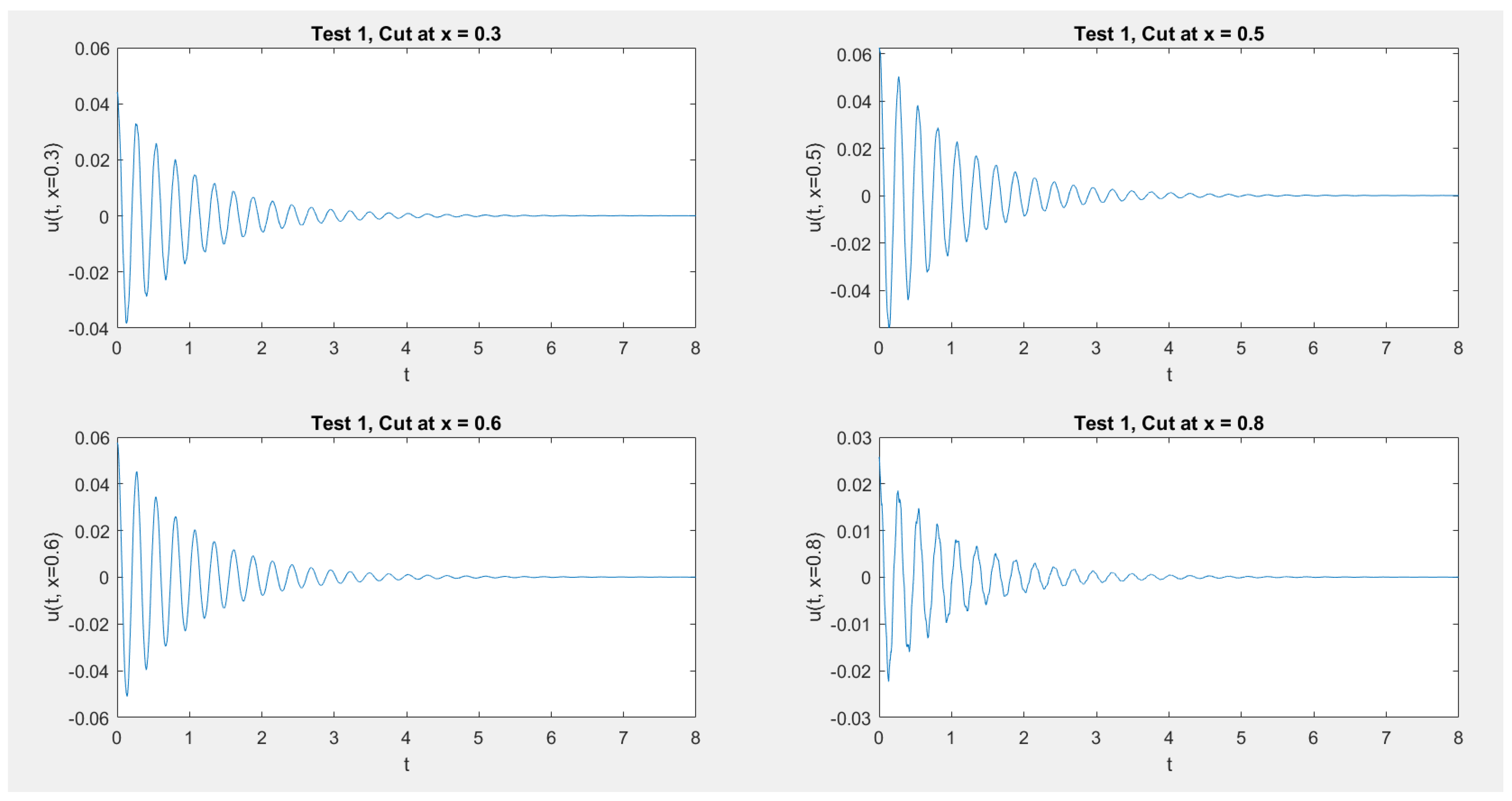
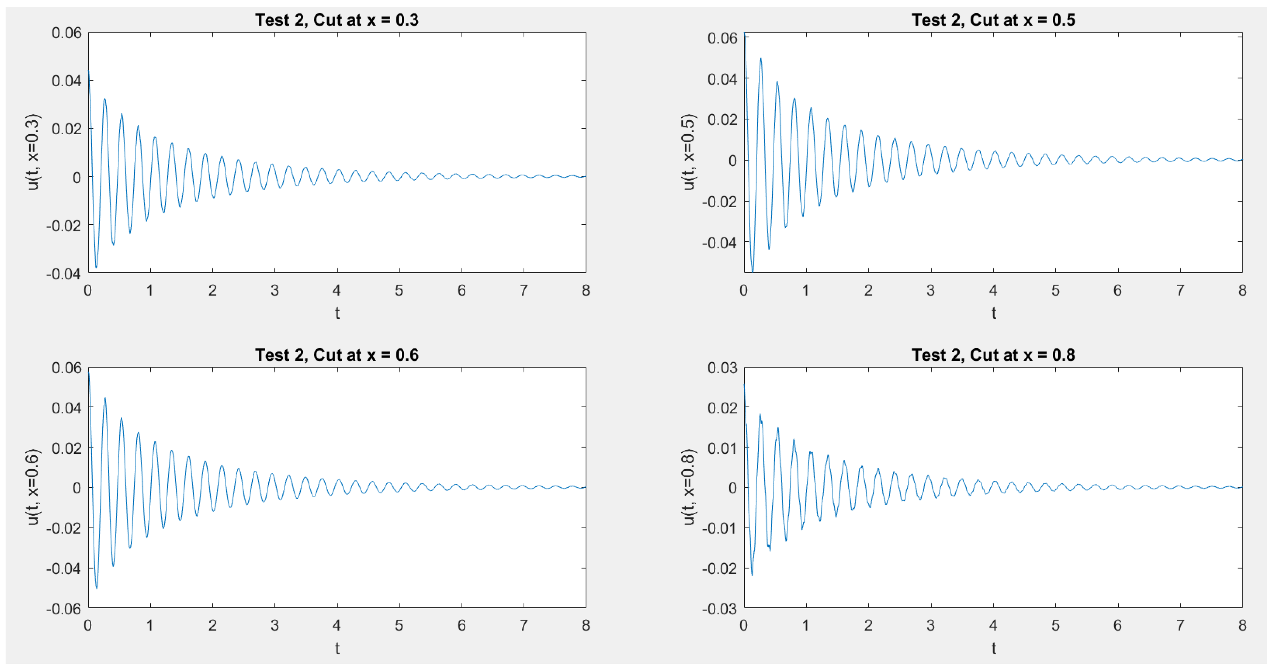
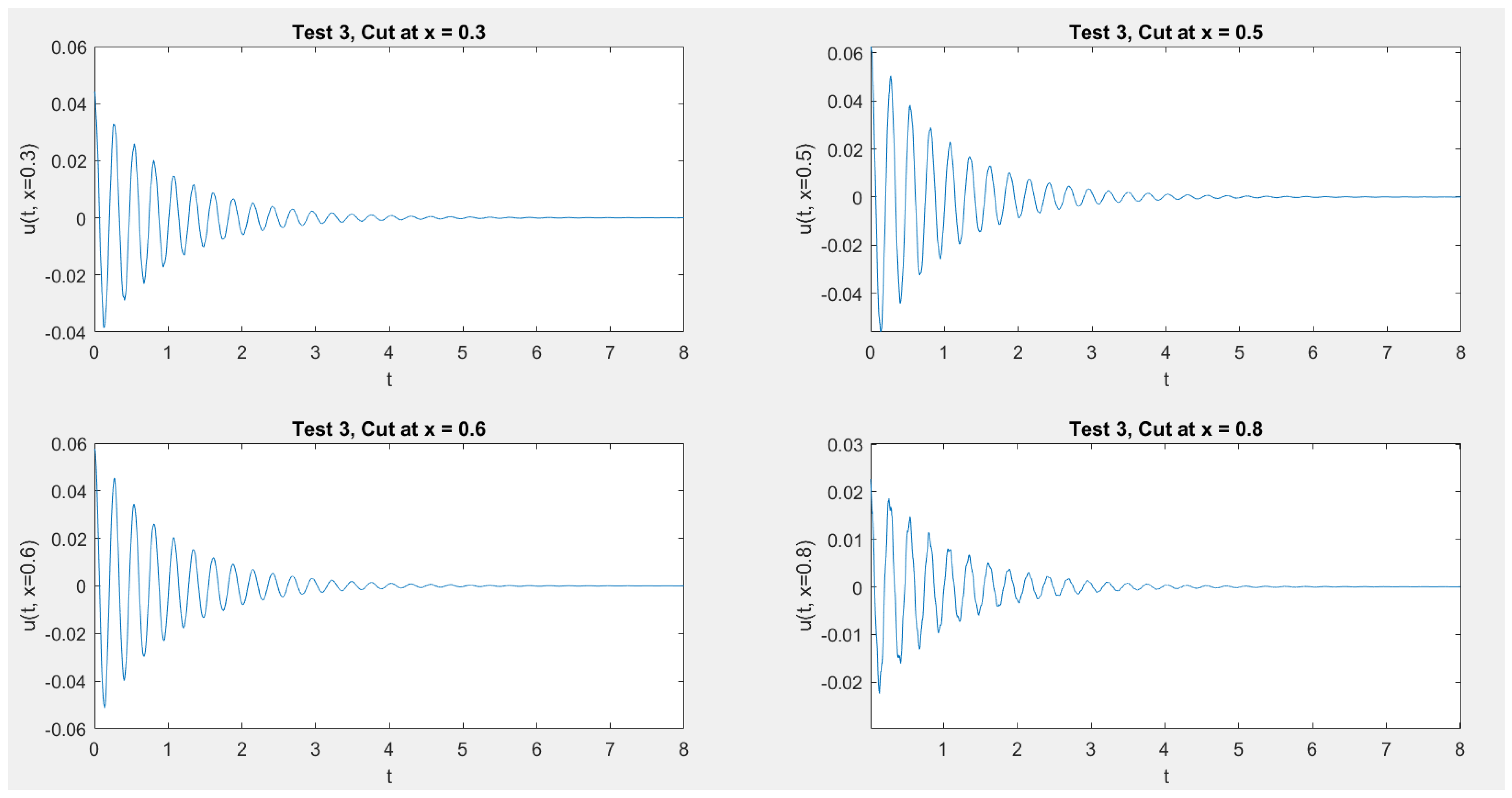
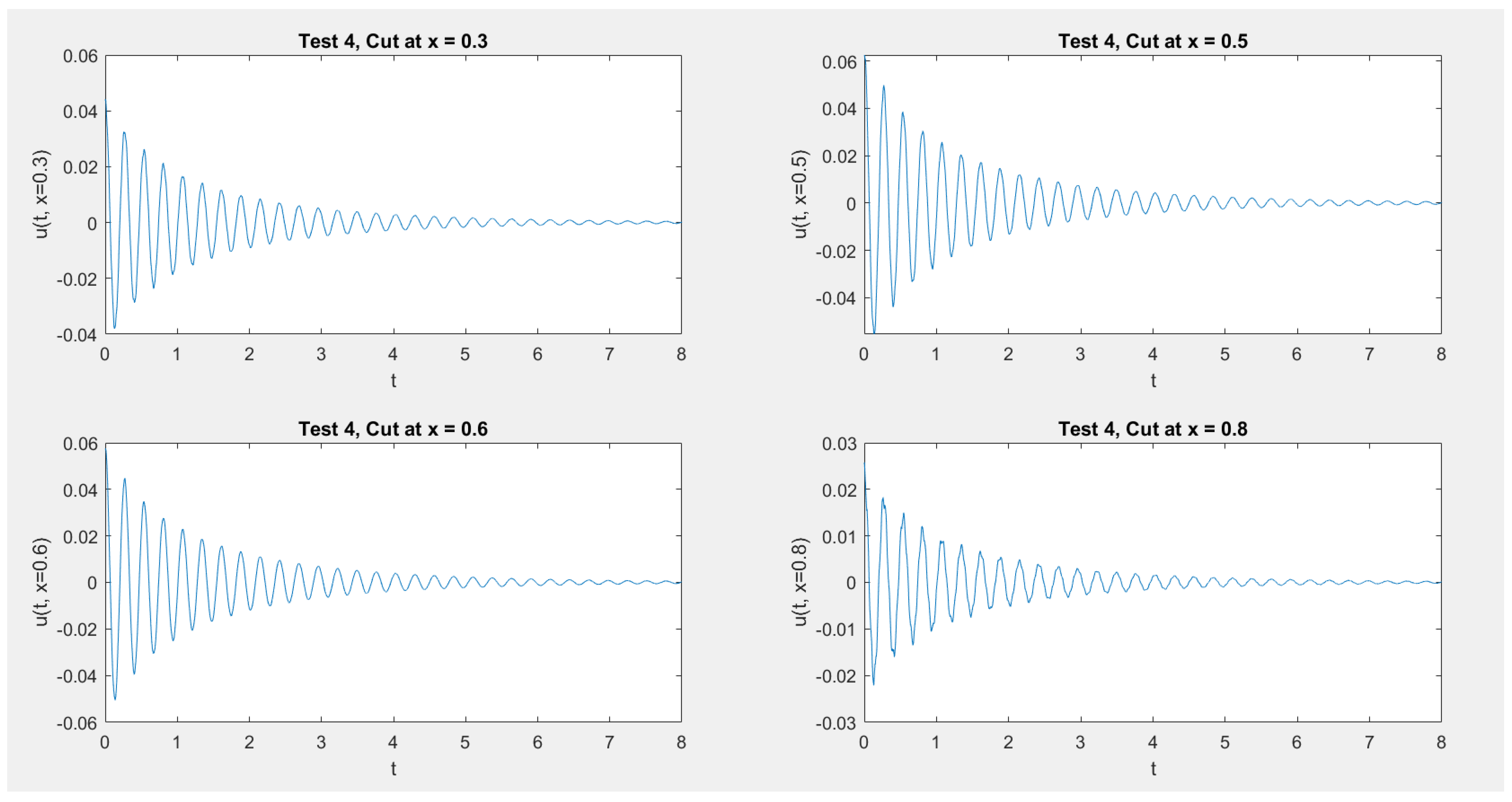
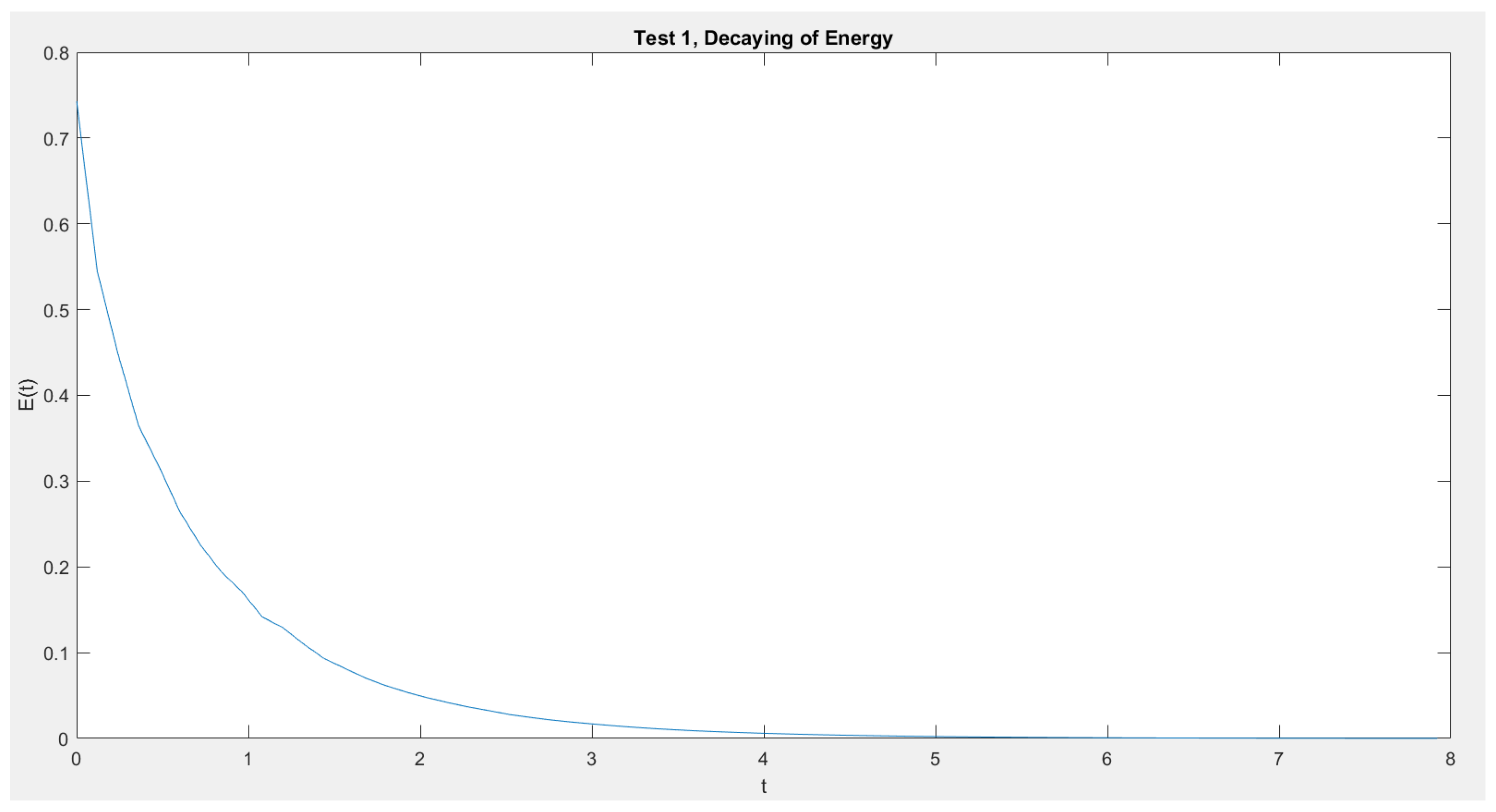
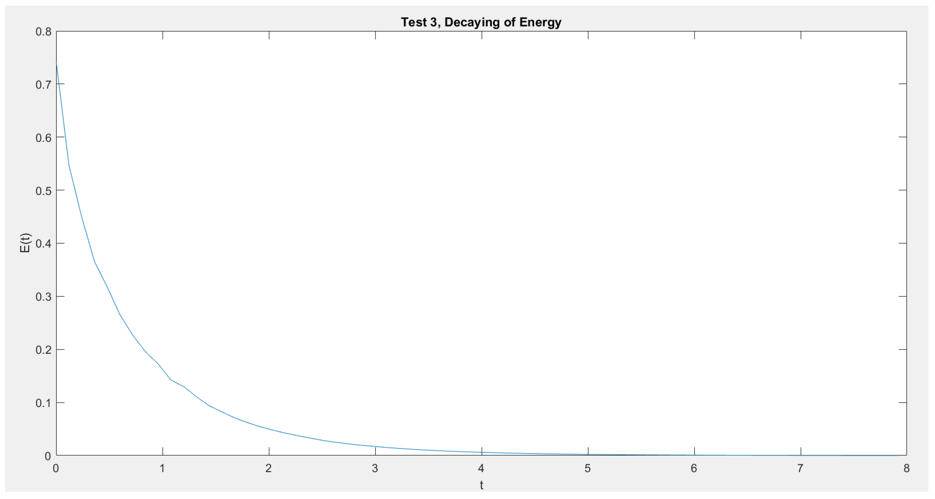
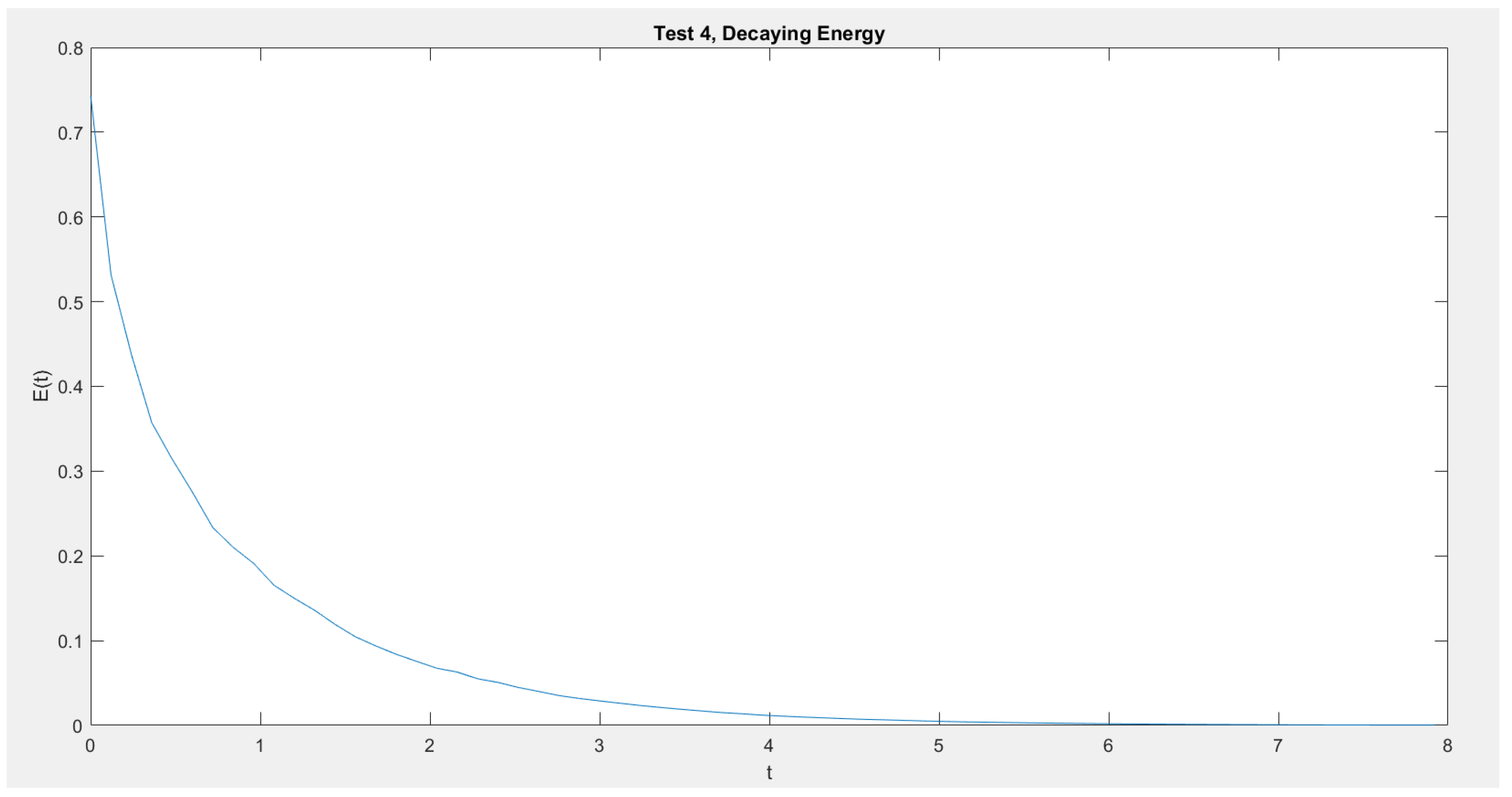
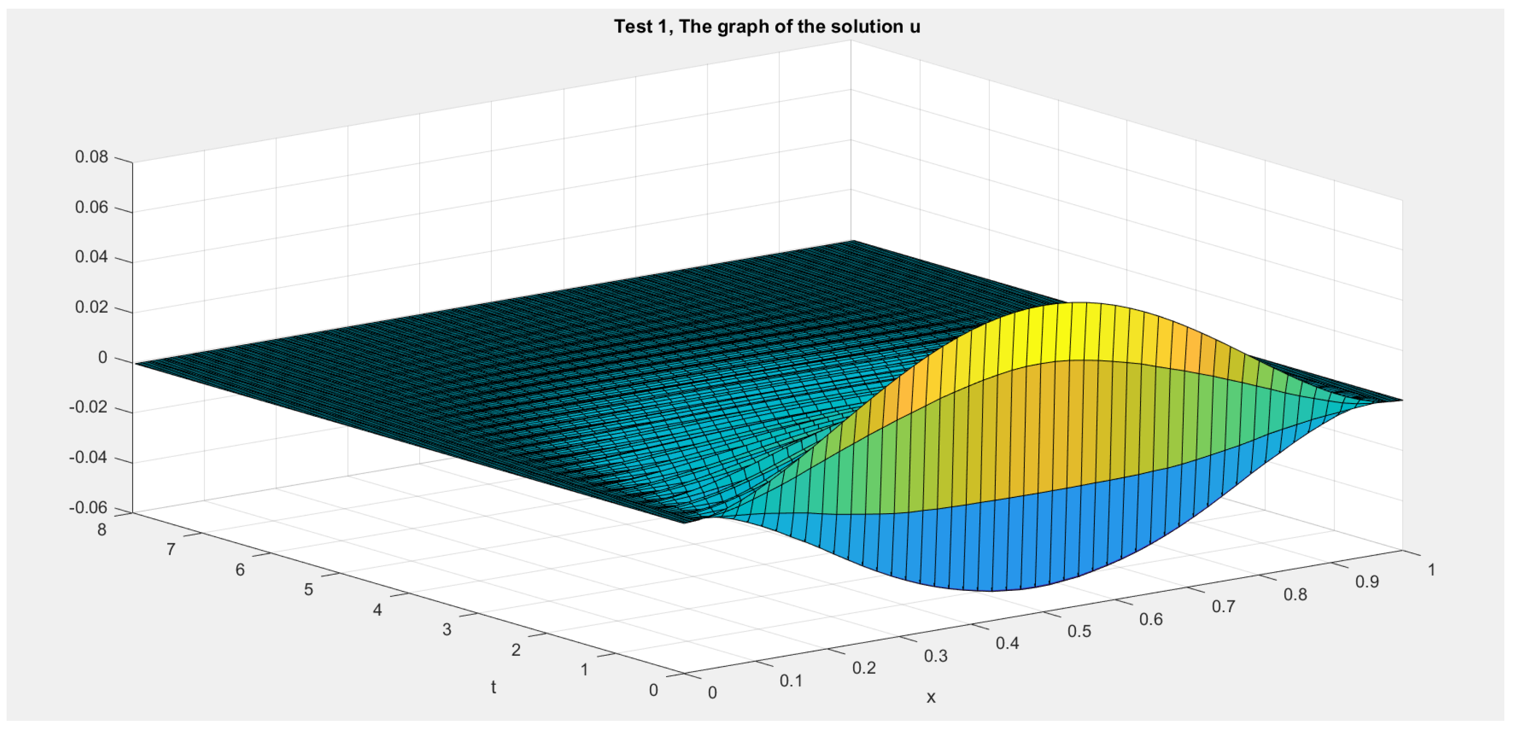
5. Numerical Results

In this section, we perform some numerical experiments to illustrate the theoretical results in Theorems 1 and 2. For this purpose, we discretize the system (9) using a finite difference method (FDM) in both time and space with second-order in time and forth-order in space for the time-space domain $[0,L]\times [0,T]=[0,1]\times [0,8]$. The spatial interval $(0,1)$ is divided into 50 subintervals, where the time interval $(0,T)$ is divided into $4\times {10}^4$ subintervals with a time step $\Delta t=\frac{T}{N}$.

The homogeneous Dirichlet boundary condition of the problem (9) is given and the normal derivative is equal to zero at the boundary using the following initial conditions:

• $u(x,0)=x^2{(1-x)}^2$
• $u_t(x,0)=0$

We compare the energy decay and the solution of problem (9) through four numerical tests based on the function h and the kernel function g.

• Test 1: We consider $h\left(u_t\right)=u_t$ and $g\left(t\right)=e^{-t}$.
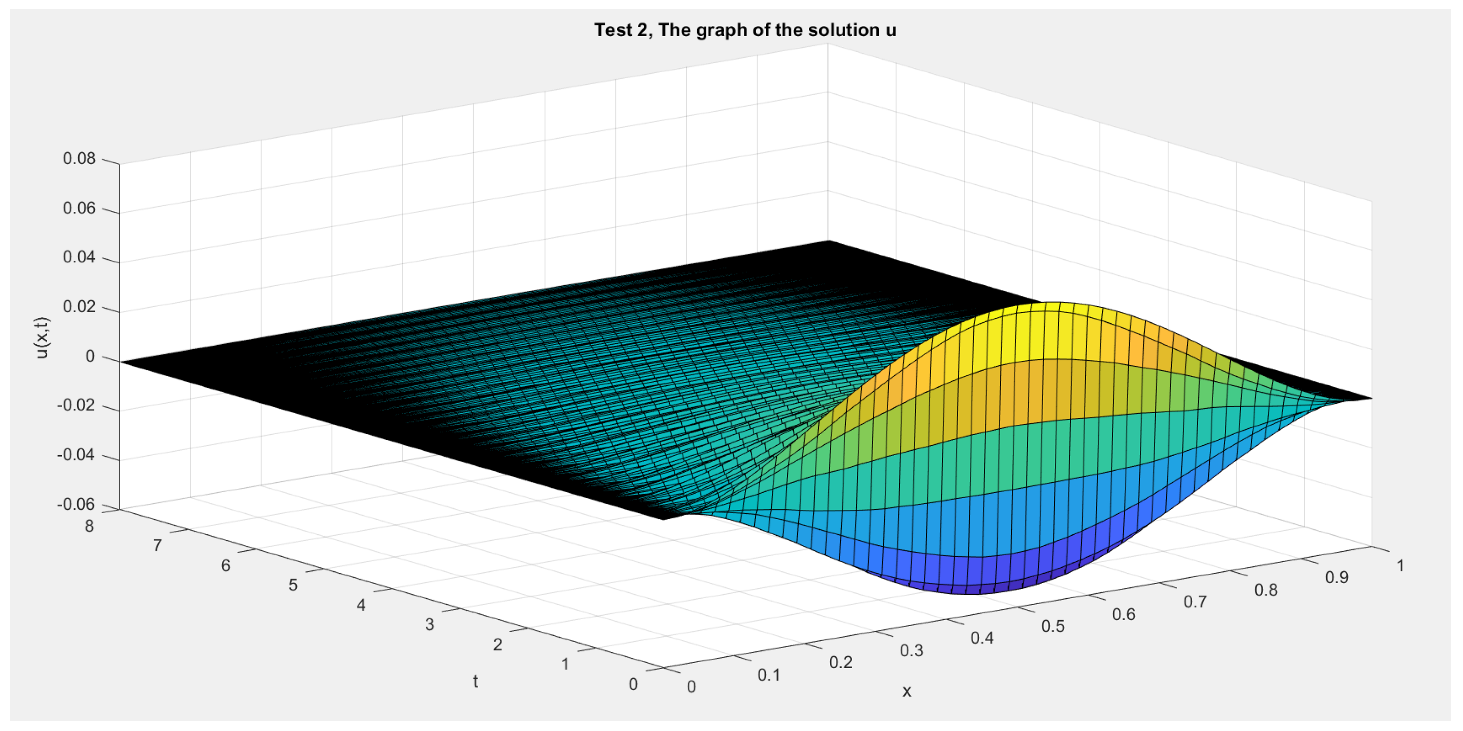
• Test 2: We consider $h\left(u_t\right)=u_t\left|u_t\right|$ and $g\left(t\right)=e^{-t}$.
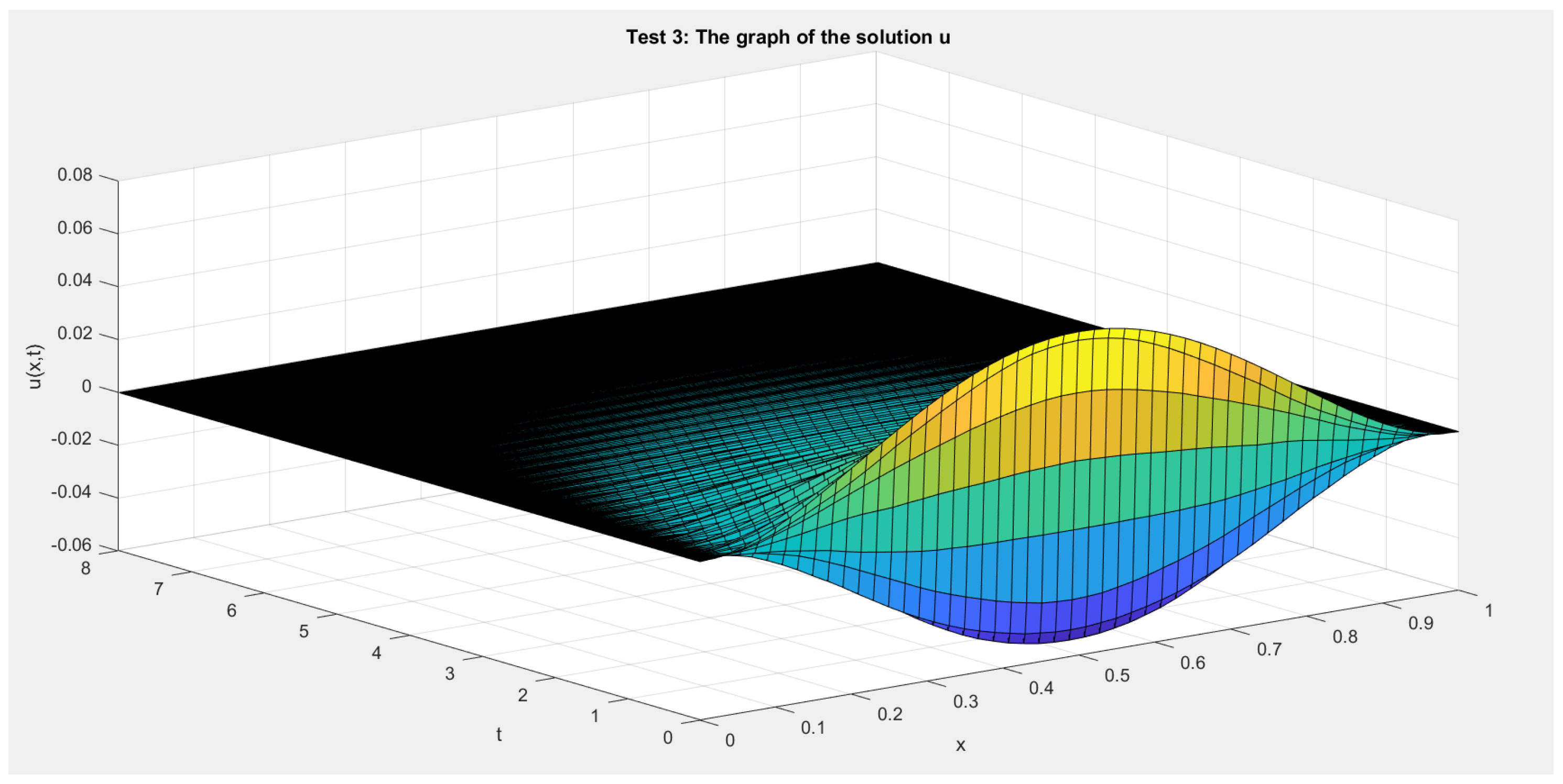
• Test 3: We consider $h\left(u_t\right)=u_t$ and $g\left(t\right)=\frac{1}{{(t+1)}^2}$
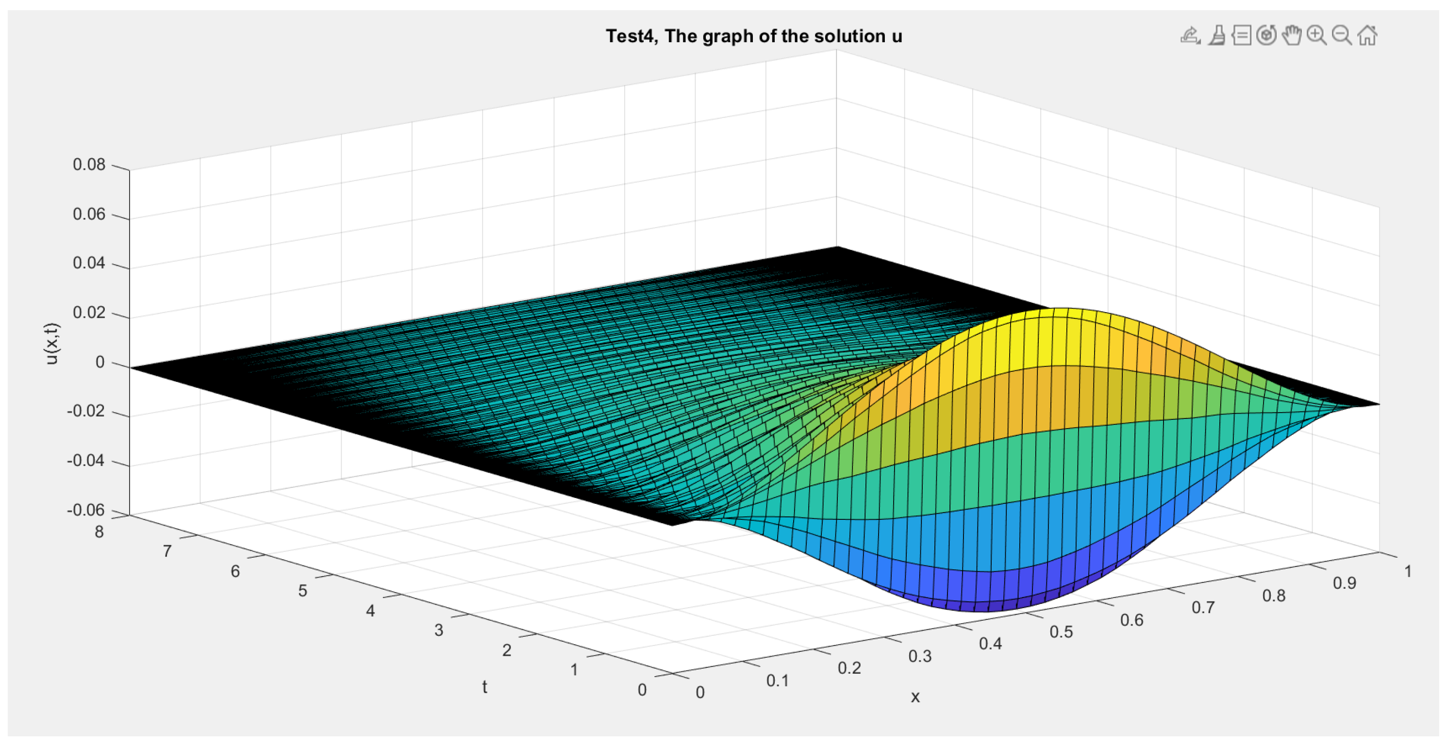
• Test 4: We consider $h\left(u_t\right)=u_t\left|u_t\right|$ and $g\left(t\right)=\frac{1}{{(t+1)}^2}$.

In Figure 1, Figure 2, Figure 3 and Figure 4 we show the cross section cuts of the approximate solution u at $x=0.3$, $x=0.5$, $x=0.6$, and $x=0.8$ for Test 1, Test 2, Test 3, and Test 4, Respectively. In Figure 5, Figure 6, Figure 7 and Figure 8 we sketch the corresponding energy functional (14). Also, we sketch the decay behavior of the whole wave over the time interval $[0,8]$ in Figure 9, Figure 10, Figure 11 and Figure 12 for Test 1 to Test 4, Respectively.

Figure 1. Test 1: The solution. $u\left(t\right)$ at fixed values of x.

Figure 2. Test 2: The solution $u\left(t\right)$ at fixed values of x.

Figure 3. Test 3: The solution $u\left(t\right)$ at fixed values of x.

Figure 4. Test 4: The solution $u\left(t\right)$ at fixed values of x.

Figure 5. Test 1: The energy decay.

Figure 6. Test 2: The energy decay.

Figure 7. Test 3: The energy decay.

Figure 8. Test 4: The energy decay.

Figure 9. Test 1: The solution $u(x,t)$.

Figure 10. Test 2: The solution $u(x,t)$.

Figure 11. Test 3: The solution $u(x,t)$.

Figure 12. Test 4: The solution $u(x,t)$.

References

- Dafermos, C.M. An abstract Volterra equation with applications to linear viscoelasticity. J. Differ. Equ. 1970, 7, 554–569. [Google Scholar] [CrossRef] [Green Version]
- Lagnese, J.E. Asymptotic energy estimates for Kirchhoff plates subject to weak viscoelastic damping. Int. Ser. Numer. Math. 1989, 91, 211–236. [Google Scholar]
- Rivera, J.M.; Lapa, E.C.; Barreto, R. Decay rates for viscoelastic plates with memory. J. Elast. 1996, 44, 61–87. [Google Scholar] [CrossRef]
- Komornik, V. On the nonlinear boundary stabilization of Kirchhoff plates. Nonlinear Differ. Equ. Appl. NoDEA 1994, 1, 323–337. [Google Scholar] [CrossRef]
- Messaoudi, S.A. Global existence and nonexistence in a system of Petrovsky. J. Math. Anal. Appl. 2002, 265, 296–308. [Google Scholar] [CrossRef] [Green Version]
- Chen, W.; Zhou, Y. Global nonexistence for a semilinear Petrovsky equation. Nonlinear Anal. Theory Methods Appl. 2009, 70, 3203–3208. [Google Scholar] [CrossRef]
- Barrow, J.D.; Parsons, P. Inflationary models with logarithmic potentials. Phys. Rev. D 1995, 52, 5576. [Google Scholar] [CrossRef] [Green Version]
- Enqvist, K.; McDonald, J. Q-balls and baryogenesis in the MSSM. Phys. Lett. B 1998, 425, 309–321. [Google Scholar] [CrossRef] [Green Version]
- Bialynicki-Birula, I.; Mycielski, J. Nonlinear wave mechanics. Ann. Phys. 1976, 100, 62–93. [Google Scholar] [CrossRef]
- Cazenave, T.; Haraux, A. Équations d’évolution avec non linéarité logarithmique. Ann. Fac. Sci. Toulouse Mathématiques 1980, 2, 21–51. [Google Scholar]
- Gorka, P. Logarithmic Klein-Gordon equation. Acta Phys. Polon. 2009, 40, 59–66. [Google Scholar]
- Al-Gharabli, M.M.; Messaoudi, S.A. Existence and a general decay result for a plate equation with nonlinear damping and a logarithmic source term. J. Evol. Equ. 2018, 18, 105–125. [Google Scholar] [CrossRef]
- Bartkowski, K.; Górka, P. One-dimensional Klein–Gordon equation with logarithmic nonlinearities. J. Phys. A Math. Theor. 2008, 41, 355201. [Google Scholar] [CrossRef]
- Hiramatsu, T.; Kawasaki, M.; Takahashi, F. Numerical study of Q-ball formation in gravity mediation. J. Cosmol. Astropart. Phys. 2010, 2010, 008. [Google Scholar] [CrossRef] [Green Version]
- Han, X. Global existence of weak solutions for a logarithmic wave equation arising from Q-ball dynamics. Bull. Korean Math. Soc. 2013, 50, 275–283. [Google Scholar] [CrossRef] [Green Version]
- Kafini, M.; Messaoudi, S. Local existence and blow up of solutions to a logarithmic nonlinear wave equation with delay. Appl. Anal. 2020, 99, 530–547. [Google Scholar] [CrossRef]
- Peyravi, A. General stability and exponential growth for a class of semi-linear wave equations with logarithmic source and memory terms. Appl. Math. Optim. 2020, 81, 545–561. [Google Scholar] [CrossRef]
- Xu, R.; Lian, W.; Kong, X.; Yang, Y. Fourth order wave equation with nonlinear strain and logarithmic nonlinearity. Appl. Numer. Math. 2019, 141, 185–205. [Google Scholar] [CrossRef]
- Lian, W.; Xu, R. Global well-posedness of nonlinear wave equation with weak and strong damping terms and logarithmic source term. Adv. Nonlinear Anal. 2019, 9, 613–632. [Google Scholar] [CrossRef]
- Wang, X.; Chen, Y.; Yang, Y.; Li, J.; Xu, R. Kirchhoff-type system with linear weak damping and logarithmic nonlinearities. Nonlinear Anal. 2019, 188, 475–499. [Google Scholar] [CrossRef]
- Al-Mahdi, A.M. Optimal decay result for Kirchhoff plate equations with nonlinear damping and very general type of relaxation functions. Bound. Value Probl. 2019, 2019, 82. [Google Scholar] [CrossRef]
- Al-Gharabli, M.M.; Al-Mahdi, A.M.; Messaoudi, S.A. Decay Results for a Viscoelastic Problem with Nonlinear Boundary Feedback and Logarithmic Source Term. J. Dyn. Control. Syst. 2020, 28, 71–89. [Google Scholar] [CrossRef]
- Al-Gharabli, M.M.; Al-Mahdi, A.M.; Kafini, M. Global existence and new decay results of a viscoelastic wave equation with variable exponent and logarithmic nonlinearities. AIMS Math. 2021, 6, 10105–10129. [Google Scholar] [CrossRef]
- Cavalcanti, M.M.; Domingos Cavalcanti, V.N.; Soriano, J.A. Exponential decay for the solution of semilinear viscoelastic wave equations with localized damping. Electron. J. Differ. Equ. (EJDE) 2002, 2002, 1–14. [Google Scholar]
- Messaoudi, S.A. General decay of the solution energy in a viscoelastic equation with a nonlinear source. Nonlinear Anal. Theory Methods Appl. 2008, 69, 2589–2598. [Google Scholar] [CrossRef]
- Messaoudi, S.A. General decay of solutions of a viscoelastic equation. J. Math. Anal. Appl. 2008, 341, 1457–1467. [Google Scholar] [CrossRef] [Green Version]
- Alabau-Boussouira, F.; Cannarsa, P. A general method for proving sharp energy decay rates for memory-dissipative evolution equations. Comptes Rendus Math. 2009, 347, 867–872. [Google Scholar] [CrossRef] [Green Version]
- Lasiecka, I.; Messaoudi, S.A.; Mustafa, M.I. Note on intrinsic decay rates for abstract wave equations with memory. J. Math. Phys. 2013, 54, 031504. [Google Scholar] [CrossRef]
- Messaoudi, S.A.; Al-Khulaifi, W. General and optimal decay for a quasilinear viscoelastic equation. Appl. Math. Lett. 2017, 66, 16–22. [Google Scholar] [CrossRef]
- Al-Gharabli, M.M.; Guesmia, A.; Messaoudi, S.A. Existence and a general decay results for a viscoelastic plate equation with a logarithmic nonlinearity. Commun. Pure Appl. Anal. 2019, 18, 159–180. [Google Scholar] [CrossRef] [Green Version]
- Mustafa, M.I. Optimal decay rates for the viscoelastic wave equation. Math. Methods Appl. Sci. 2018, 41, 192–204. [Google Scholar] [CrossRef]
- Gross, L. Logarithmic sobolev inequalities. Am. J. Math. 1975, 97, 1061–1083. [Google Scholar] [CrossRef]
- Chen, H.; Luo, P.; Liu, G. Global solution and blow-up of a semilinear heat equation with logarithmic nonlinearity. J. Math. Anal. Appl. 2015, 422, 84–98. [Google Scholar] [CrossRef]
- Al-Gharabli, M.M.; Al-Mahdi, A.M.; Messaoudi, S.A. General and optimal decay result for a viscoelastic problem with nonlinear boundary feedback. J. Dyn. Control Syst. 2019, 25, 551–572. [Google Scholar] [CrossRef]
- Arnol’d, V.I. Mathematical Methods of Classical Mechanics; Springer Science & Business Media: Berlin/Heidelberg, Germany, 2013; Volume 60. [Google Scholar]
Publisher’s Note: MDPI stays neutral with regard to jurisdictional claims in published maps and institutional affiliations. |
© 2022 by the authors. Licensee MDPI, Basel, Switzerland. This article is an open access article distributed under the terms and conditions of the Creative Commons Attribution (CC BY) license (https://creativecommons.org/licenses/by/4.0/).
Share and Cite
Al-Gharabli, M.M.; Almahdi, A.M.; Noor, M.; Audu, J.D. Numerical and Theoretical Stability Study of a Viscoelastic Plate Equation with Nonlinear Frictional Damping Term and a Logarithmic Source Term. Math. Comput. Appl. 2022, 27, 10. https://doi.org/10.3390/mca27010010
Al-Gharabli MM, Almahdi AM, Noor M, Audu JD. Numerical and Theoretical Stability Study of a Viscoelastic Plate Equation with Nonlinear Frictional Damping Term and a Logarithmic Source Term. Mathematical and Computational Applications. 2022; 27(1):10. https://doi.org/10.3390/mca27010010
Chicago/Turabian StyleAl-Gharabli, Mohammad M., Adel M. Almahdi, Maher Noor, and Johnson D. Audu. 2022. "Numerical and Theoretical Stability Study of a Viscoelastic Plate Equation with Nonlinear Frictional Damping Term and a Logarithmic Source Term" Mathematical and Computational Applications 27, no. 1: 10. https://doi.org/10.3390/mca27010010