
Meshless Computational Strategy for Higher Order Strain Gradient Plate Models
by
 , , , and
Francesco Fabbrocino
1 ,
,
Serena Saitta
1,
Riccardo Vescovini
2,
Nicholas Fantuzzi
3,* and
and
Raimondo Luciano
4 1
Department of Engineering, Telematic University Pegaso, Centro Direzionale Isola F2, 80143 Napoli, Italy
2
Department of Aerospace Science and Technology, Politecnico di Milano, Via La Masa 34, 20156 Milano, Italy
3
Department of Civil, Chemical, Environmental, and Materials Engineering, University of Bologna, Viale del Risorgimento 2, 40136 Bologna, Italy
4
Department of Engineering, Parthenope University, Centro Direzionale Isola C4, 80133 Napoli, Italy
*
Author to whom correspondence should be addressed.
Math. Comput. Appl. 2022, 27(2), 19; https://doi.org/10.3390/mca27020019
Submission received: 24 January 2022
/
Revised: 14 February 2022
/
Accepted: 21 February 2022
/
Published: 22 February 2022
(This article belongs to the Special Issue Mathematical and Computational Modelling in Mechanics of Materials and Structures)
Abstract
:The present research focuses on the use of a meshless method for the solution of nanoplates by considering strain gradient thin plate theory. Unlike the most common finite element method, meshless methods do not rely on a domain decomposition. In the present approach approximating functions at collocation nodes are obtained by using radial basis functions which depend on shape parameters. The selection of such parameters can strongly influences the accuracy of the numerical technique. Therefore the authors are presenting some numerical benchmarks which involve the solution of nanoplates by employing an optimization approach for the evaluation of the undetermined shape parameters. Stability is discussed as well as numerical reliability against solutions taken for the existing literature.
1. Introduction
In the broad context of meshless methods Meshless Local Petrov–Galerkin (MLPG) [1] demonstrated to have strong capabilities to solve problems where weakly-singular traction and displacement boundary integral equations are involved. Moreover, other problems in this context have been analyzed and solved [2,3]. The main idea of meshless methods is to go beyond the current limitations of finite element models for analyzing problems in mechanics [4]. Unlike classical FEM shape functions are developed for a scattered set of collocation nodes [4,5] and their generation defines different meshless approaches. The one considered in the present work is named Radial Point Interpolation Method (RPIM) [6,7,8,9] which has the fundamental property of Kronecker delta function [10,11,12,13]. This approach makes the RPIM extremely easy to be implemented and used for the solution of any problem in structural mechanics.
It has been demonstrated to be extremely relevant in industrial applications for nanoengineering that nanoelectromechanical (NEMS) systems have been widely considered in the recent literature with several gradient elasticity problems [14,15]. It has been demonstrated in recent literature that nano-structures are used for micro-sized systems and devices such as biosensors, nano-actuators and nano-electro-mechanical systems [16].
Among the vast literature of nonlocal theories stress-driven models have been recently presented for nanobeams presenting analytical solutions. For instance closed-form solution of Bernoulli and Timoshenko type for Erigen-like formulations and stress field and a bi-exponential averaging kernel functions characterized by a scale parameter is presented in [17,18,19]. Nonlocal strain gradient Bernoulli like beam models by considering special bi-exponential averaging kernels and functionally graded materials has been presented in [20]. Nonlocal beam formulations have been presented within a thermodynamic framework, variational formulation within its analytical solution has been provided in [21]. Nanobeams can be subjected to axial loads which leads to buckling, such effects must be considered for a proper nanoengineering design, thus stress-driven buckling of nanobeams can be found in [22,23]. In the context of dynamic problems vibrations in nonlocal integral elasticity has been recently considered for beams and plates in [24,25].
Most of the nonlocal theories relies on homogenization approaches which aim at simplifying the problem by considering less modelling parameters in composite materials [26,27]. It is remarked that size effects and microstructures paved the way in presenting innovative and multiscale approches in solid mechanics [28,29].
It has been demonstrated by several researchers that higher-order elasticity is becoming of paramount importance for solid mechanics as mentioned in [30,31,32]. In most researchers the term nonlocality has been brought by Eringen [33] and by Eringen and Edelen [34] where it can be found that the constitutive relations have to be modified to take into account their dependency on the mechanical properties of the entire body and not only of the properties in the neighborhood of the material point. In this regard, in the present work nonlocal effects have be meaning introduced by Altan and Aifantis [35,36], which considered a simplified nonlocal model where all nonlocalities are concentrated in a gradient model similar to the one proposed by Mindlin [37]. Such approach, known as strain gradient theory, has been utilized also by others in other contexts in solid mechanics [38,39,40]. Strain gradient theory [41] has been demonstrated to be a constrained version of other higher-order unconstrained versions available in the literature such as couple stress [42,43,44] as well as micropolar theories [45,46,47].
In the framework of plate theories thin plate model is very common within the area of structural mechanics of investigating thin-walled structures [48,49]. Such approach can be easily extended in order to consider composite structures such as laminated [50,51] or sandwich ones [52].
To this day, the application of Mesh Free Methods for the analysis of structures modeled according to the strain gradient theory appears to be limited. Static analysis as well as buckling and free vibration of strain gradient beams and plates have been studied by means of different Mesh Free techniques [53,54,55,56]. However, none of the works mentioned makes use of the Mesh Free RPIM to perform the analysis.
In the present work the advantages of meshless methods are considered in the framework of strain gradient composite thin plate theory to solve such numerical problem.
2. Theoretical Background
The present work considers the problem of laminated thin plates of rectangular plane form of size , where indicate lengths with respect to , respectively. The plate thickness is indicated with h and the plate represents the middle plane of the actual plate with z axis pointed normal to the plate. Each ply which constitutes the stacking sequence is indicated with and the total thickness is computed as , where denotes the number of plies [57].
The present displacement field follows the classical thin plate theory and Cartesian displacements can be represented as [58]
where is the vector collecting the three middle plane displacements of the material point and is the derivative operation defined in [59]. The strain vector is given by
in which and denote respectively the membrane and bending strains, respectively. They can be evaluated as follows
where the meaning of the differential operators , is reported in [58,59].
Linear constitutive law is considered within the strain gradient theory as suggested in [40] allows to relate the membrane stresses in the k-th layer to the corresponding strain components as shown below [60,61]
in which the nonlocal parameter ℓ includes the micro/macro-scale interaction effects. The dependency of the stresses on the strain distribution within the medium is emphasized by the presence of the Laplacian in Cartesian coordinate system: . On the other hand, represents the plane stress-reduced stiffness coefficients matrix of the k-th layer. The terms of this matrix depend on the orthotropic properties of the layer (Young’s moduli , , Poisson’s ratio and shear modulus ), as well as by an arbitrary orientation as indicated in the book [62]. the and are the stress resultants that can be defined as follows
The differential operators , , , are defined in [58]. The constitutive operators , , represent instead the membrane, membrane-bending coupling and bending stiffness matrices of the laminated composite plates [62].
In the current paper, isotropic and composite schemes are considered, therefore for some configurations , thus, membrane and bending behaviors are coupled. The variational form of the present equilibrium is represented by [58,63]
The present meshless technique is applied to such variational statements of the problem.
3. Mesh Free Methods
The present numerical solution is obtained using a Mesh Free approach.
As explained in detail in [4], with respect to traditional FEM, the two methods diverge at the stage of geometry discretization. In conventional FEM, the continuum is discretized by means of a mesh which also introduces predefined relationship between the nodes. Shape functions and system equations are then written for each element in the mesh.
In a Mesh Free method the domain is not discretized. It is represented by a set of nodes scattered in the domain and on its boundaries. Since no elements exist in this description, the shape functions and the system equations are written for the nodes. This characteristics allows to introduce a huge degree of flexibility, with respect to FEM, in term of adding or removing nodes from the domain.
The absence of the mesh implies the the relationship between the nodes representing the domain are not defined a priori. Therefore, a new concept has to be introduced to explain how the shape functions are constructed.
In Mesh Free methods, the field variable is interpolated using only the nodes falling within a local domain, within the problem domain, called support domain. The support domain can have different shapes, the most common being circular or rectangular, the latter being the choice for this work. The numerical procedure for the shape functions calculation is as follows. The support domain is first centered in a point of interest. The nodes falling inside it are identified and the shape functions are constructed using only those nodes. Once all the necessary calculations are performed, the support domain is moved to be centered in the next point of interest and the procedure starts anew. The so-called point of interest in which this local domain is centered can be either a node or, as chosen for this work, a Gauss point.
It has been explained how in mesh free methods the domain is represented by a set of scattered nodes rather than discretized by means of a mesh. Hence, it may seem contradictory to talk about Gauss points in such context. As a matter of fact, the Gauss points come from the necessity of numerically evaluate the integrals appearing in the weak form of the equation of motion, as shown in Equation (6).
For the sole purpose of integrals evaluation, in fact, a so-called background mesh needs to be introduced. The background mesh and nodal distribution are two independent objects, as shown in Figure 1, and its sole purpose is the integrals evaluation.
As stated, the only nodes used to construct the shape functions are the ones falling within the support domain of the i-th point of interest. It follows that the size of the support domain is an important aspect to ensure that the shape functions are computed properly. The size of the local domain is evaluated as:
where is the average nodal spacing and is a nondimensional parameter.
This parameter has to be tuned to ensure that the appropriate amount of nodes is contained within the support domain.
4. Radial Point Interpolation Method (RPIM)
In the present approach solution is obtained in scattered points located in the given plate rectangular domain. The approximating polynomials involved possess the Kronecker delta property which allows a straightforward implementation of boundary conditions. In the following implementation, in plane displacements u and v, transverse displacement w as well as rotations , are included in the numerical implementation even though more primary variables are involved in the present formulation [58,59].
Since both isotropic and laminated plates are studied, the degrees of freedom for the different cases are taken as shown in Table 1. In the context of the strain gradient theory, the essential boundary conditions for the plate are shown in Table 2 where the four edges are identified by the values of the physical coordinates x and y.
Any other higher-order derivative is carried out by numerical derivation of the aforementioned parameters. Since both the deflection and its first derivatives are considered unknown, the Hermite–RPIM formulation is here presented. Let’s consider a domain enclosing n arbitrarily scattered nodes. The approximation of the generic displacement can be expressed as:
where , and are the vectors including the radial basis functions (RBF) and their derivatives. The correspondent coefficients are indicated using vectors , and . For the following numerical applications the well-known multi-quadrics (MQ) RBF is used in its general form
where . Both q and are shape parameters that have to be tuned while is the average nodal spacing.
The vectors of coefficients in Equation (8) can be obtained by enforcing the field function and its derivatives to be satisfied at all the n nodes falling within the support domain of the point of interest . The support domain is a local domain, typically circular or rectangular, centered in a point of interest which can either be a node or an integration point.
This leads to linear equations
where is a vector containing the function values of the degrees of freedom considered in the collocation nodes and listed in Table 1. Thus, the independent parameter can be carried out as
An example of what the shape functions look like as computed with this method is given in Figure 2. A squared domain, represented by regularly distributed nodes, is considered and all of the nodes are used to construct the shape functions for this domain. Figure 2, Figure 3 and Figure 4 represent the shape functions and their first derivatives with respect to x and y for the nodes in the bottom left corner, in the middle left side, in the middle of the domain and in the top right corner, respectively. For this particular case, the dimensionless parameters of the RBF are chosen as and .
By following the same computational strategy of conventional finite element method [58] the algebraic form of the variational statement can be carried out because shape functions are evaluated at the collocation nodes. The needed integration is performed by following well-known Gauss integration rules. Solution of the present static problem is provided by Gauss elimination algorithm. The following section is dedicated to numerical results, stability and accuracy.
5. Applications
In the following sections, the numerical results of the analysis are shown and commented. Discussion about the degrees of freedom taken as variables in the problem and numerical convergence analysis are introduced, as well as plots of both convergence and deformed configurations which are also reported for clarity of representation.
5.1. Isotropic Plates
This section shows the results of the numerical analysis of isotropic Kirchhoff nanoplates modeled according to the second-order strain gradient theory and analyzed by means of a mesh free RPIM. In this case, there is no coupling between the in plane and out of plane behavior. Hence, the only unknown variables considered in the numerical implementation the are transverse displacement w and the corresponding rotations , . The numerical codes are developed in MATLAB.
The results in terms of mid transverse displacement are presented in the non-dimensional form as follows:
where w is the central plate deflection, is the magnitude of the transverse external load and D is the bending rigidity .
Squared nanoplates with different constraints are analyzed, all having thickness nm. Young’s modulus and Poisson’s ratio are taken as 1100 GPa and , respectively. Five different combinations of boundary conditions are accounted for, namely SSSS, CCCC, SCSC, SFSF, SCSF.
Different nodal densities are also taken into account. Nanoplates represented by , , and equally spaced node grids are studied to analyze the convergence of the method. The non-local parameter ℓ also varies according to the analysis and results presented in the available literature [64].
The support domain used for the mesh free implementation has rectangular shape and is centered in the Gauss points. Its dimensions are considered in the classical way [4] where is the average nodal spacing and is a dimensionless parameter which, in this work, varies from 2 to 3. Note that, in this work, Gauss integration points are used in each cell of the background integration mesh.
Results listed in Table 3, Table 4, Table 5 and Table 6 compare the available analytical solutions [64] with the present ones in terms of percentage error:
where is the exact solution taken from the aforementioned references.
The provided comparison is performed for different boundary conditions, number of collocation nodes and non-local parameter values.
As mentioned, in Mesh Free methods the background mesh and nodal distribution which represents the domain are two independent objects. However, in this work, the analysis is performed considering the collocation nodes to be coincident with nodes of the background mesh. This choice influences the convergence analysis in terms of mesh refinement. A small number of nodes implies a coarser background mesh while high number of nodes implies a finer mesh.
The and q coefficients characterizing the MQ radial basis functions, as well as the non-dimensional support domain parameter, vary as the number of nodes changes. On the contrary, they have been kept constant as the boundary conditions change. This choice, although not very convenient, is made to show how the accuracy of the results changes based only on the number of nodes used to represent the domain and on how refined the background mesh is. The parameters are changed to provide the most suitable set for the specific nodal distribution, so that the analysis is performed under some of the best achievable conditions in each case. It is true that an optimal combination of shape parameters may be found for all the different nodal distributions considered, but its application on the different nodal densities will introduce new sources of error. Therefore, in this work, we only focus on the influence that the nodal density and the integration have on the accuracy of the results, while performing the analysis with the most convenient set of parameters in each case.
In addition, a visualization of the convergence trend is shown in Figure 5 as well as a visualization of the deformed configuration of the nanoplates here analyzed shown in Figure 6.
Observing the results, it should be remarked that while in the case of the non-local parameter the results converge monotonically in most of the cases, this trend is no longer followed as the value assumed by ℓ changes. To explain this behavior, it is necessary to acknowledge the relative influence that both the nodal coordinates and the nodal density have on the numerical results.
In a case as the one under analysis, of a plate with fixed geometry, it comes natural to understand that representing the problem domain with a small or large number of nodes influences the accuracy of the results. In mesh free methods, this numerical phenomenon occurs because the nodal spacing directly enters the calculation of derivatives of any order. As explained in previous sections, the strain gradient theory requires the computation of high order derivatives of the RBF. This implies that the spacial coordinates of the nodes are multiplied several times, once per each derivative order, for each other. For small nodal densities, meaning less nodes, these coordinates have larger values which implies that larger numbers appear in the shape functions. However, as the nodal density increases, the coordinates of the nodes get smaller and smaller. When these numbers enter the shape functions, they yields larger errors. The balancing of these two aspects, nodal density and magnitude of the nodal coordinates, may cause the alteration in the trend exhibited by the convergence.
Overall, results of the analysis are quite accurate, never reaching error value for the highest nodal density. As expected, the errors increase as the value of the non-local parameter increases, for the reason mentioned above.
5.2. Composite Plates
A similar analysis is also performed on squared cross-ply laminates.
Simply-supported (SSSS) laminates with lamination schemes 0, , and , subjected to a sinusoidal load are analyzed. The material property used are taken as , , . Moreover, the thickness is given by . As in the previous section, the results are compared in terms of non-dimensional mid-deflection:
where is the magnitude of the sinusoidal load, taken as 1. The analysis is performed using regularly distributed nodes to represent the domain and Gauss points to perform the numerical integration. The results of the analysis, compared in terms of percentage error as shown in Equation (13), are shown in Table 7.
In this case, since the nodal density is kept constant, there is no need to change the values of the non-dimensional parameters.
Even in this case, the values of the percentage error remain contained, never even reaching .
6. Conclusions
In this work, strain gradient nanoplates, both isotropic and laminated, have been analyzed by means of the Radial Point Interpolation Method. The aim was to apply a RPIM formulation to thin plates modeled via strain gradient theory. The paper provides detailed theoretical notions on mesh free methods in general as well as accurate explanation on the RPIM theoretical and numerical implementation. Moreover, theoretical notions are here reported in both explicit and matrix formulation.
This work proves the validity of the RPIM for problems with higher order of derivatives involved. Isotropic second order strain gradient Kirchhoff nanoplates with various boundary conditions are first analyzed. More specifically, SSSS, CCCC, SCSC, SFSF and SCSF boundary conditions are accounted for. Numerical convergence with the analytical results achieved in recent literature was studied. Results variation as the non-local parameter ℓ, introduced by the strain gradient theory, varies has also been studied. In a similar way, cross-ply composite plates subjected to a sinusoidal load are also analyzed. In this case, nodes are used to represent the domain and different lamination sequences are considered. The paper provides a detailed explanation of the RPIM method theoretical and numerical implementation as well as theoretical notions in both explicit and matrix form. This work proves the validity of the RPIM for problems with higher order of derivatives involved.
Author Contributions
Conceptualization, S.S. and N.F.; methodology, S.S. and R.V.; software, S.S. and R.V.; validation, S.S. and N.F.; formal analysis, S.S.; investigation, S.S.; resources, N.F.; data curation, S.S.; writing—original draft preparation, S.S. and N.F.; writing—review and editing, F.F., S.S., R.V., N.F. and R.L.; visualization, F.F., R.V. and R.L.; supervision, F.F., R.V., N.F. and R.L.; project administration, F.F. and R.L.; funding acquisition, F.F. and R.L. All authors have read and agreed to the published version of the manuscript.
Funding
This research received no external funding.
Conflicts of Interest
The authors declare no conflict of interest.
References
- Atluri, S.; Han, Z.; Shen, S. Meshless Local Petrov–Galerkin (MLPG) approaches for solving the weakly-singular traction and displacement boundary integral equations. Comput. Model. Eng. Sci. 2003, 4, 507–518. [Google Scholar]
- Atluri, S.N.; Zhu, T. A new meshless local Petrov–Galerkin (MLPG) approach in computational mechanics. Comput. Mech. 1998, 22, 117–127. [Google Scholar] [CrossRef]
- Atluri, S.N. The Meshless Method (MLPG) for Domain & BIE Discretizations; Tech Science Press: Henderson, NV, USA, 2004; Volume 677. [Google Scholar]
- Liu, G.R. Mesh Free Methods Moving beyond the Finite Element Method; CRC Press LLC: Boca Raton, FL, USA, 2003. [Google Scholar]
- Liu, G.; Gu, Y. An Introduction to Meshfree Methods and Their Programming; Springer: Amsterdam, The Netherland, 2005. [Google Scholar]
- Cui, X.; Liu, G.; Li, G. A smoothed Hermite radial point interpolation method for thin plate analysis. Arch. Appl. Mech. 2011, 81, 1–18. [Google Scholar] [CrossRef]
- Wang, J.G.; Liu, G.R. A point interpolation meshless method based on radial basis functions. Int. J. Numer. Meth. Engng. 2002, 54, 1623–1648. [Google Scholar] [CrossRef]
- Liu, G.R.; Zhang, G.Y.; Gu, Y.T.; Wang, Y.Y. A meshfree radial point interpolation method (RPIM) for three-dimensional solids. Comput. Mech. 2005, 36, 421–430. [Google Scholar] [CrossRef]
- Li, Y.; Liu, G.; Feng, Z.; Ng, K.; Li, S. A node-based smoothed radial point interpolation method with linear strain fields for vibration analysis of solids. Eng. Anal. Bound. Elem. 2020, 114, 8–22. [Google Scholar] [CrossRef]
- Gu, Y.T.; Liu, G.R. A local point interpolation method for static and dynamic analysis of thin beams. Comput. Methods Appl. Mech. Engrg. 2001, 190, 5515–5528. [Google Scholar] [CrossRef] [Green Version]
- Liu, G.R.; Gu, Y.T. A point interpolation method for two-dimensional solids. Int. J. Numer. Meth. Engng. 2001, 50, 937–951. [Google Scholar] [CrossRef]
- Liu, G.R.; Xu, X.; Zhang, G.Y.; Gu, Y.T. An extended Galerkin weak form and a point interpolation method with continuous strain field and superconvergence using triangular mesh. Comput. Mech. 2009, 43, 651–673. [Google Scholar] [CrossRef]
- Xu, X.; Liu, G.R.; Gu, Y.T.; Zhang, G.Y.; Luo, J.W.; Peng, J.X. A point interpolation method with locally smoothed strain field (PIM-LS2) for mechanics problems using triangular mesh. Finite Elem. Anal. Des. 2010, 46, 862–874. [Google Scholar] [CrossRef]
- Monaco, G.T.; Fantuzzi, N.; Fabbrocino, F.; Luciano, R. Critical Temperatures for Vibrations and Buckling of Magneto-Electro-Elastic Nonlocal Strain Gradient Plates. Nanomaterials 2021, 11, 87. [Google Scholar] [CrossRef]
- Monaco, G.T.; Fantuzzi, N.; Fabbrocino, F.; Luciano, R. Trigonometric solution for the bending analysis of magneto-electro-elastic strain gradient nonlocal nanoplates in hygro-thermal environment. Mathematics 2021, 9, 567. [Google Scholar] [CrossRef]
- Chandel, V.S.; Wang, G.; Talha, M. Advances in modelling and analysis of nano structures: A review. Nanotechnol. Rev. 2020, 9, 230–258. [Google Scholar] [CrossRef]
- Barretta, R.; Fazelzadeh, S.; Feo, L.; Ghavanloo, E.; Luciano, R. Nonlocal inflected nano-beams: A stress-driven approach of bi-Helmholtz type. Compos. Struct. 2018, 200, 239–245. [Google Scholar] [CrossRef]
- Barretta, R.; Caporale, A.; Faghidian, S.A.; Luciano, R.; Marotti de Sciarra, F.; Medaglia, C.M. A stress-driven local-nonlocal mixture model for Timoshenko nano-beams. Compos. Part B Eng. 2019, 164, 590–598. [Google Scholar] [CrossRef]
- Numanoglu, H.; Ersoy, H.; Civalek, O.; Ferreira, A. Derivation of nonlocal FEM formulation for thermo-elastic Timoshenko beams on elastic matrix. Compos. Struct. 2021, 273, 114292. [Google Scholar] [CrossRef]
- Apuzzo, A.; Barretta, R.; Fabbrocino, F.; Faghidian, S.A.; Luciano, R.; Marotti de Sciarra, F. Axial and Torsional Free Vibrations of Elastic Nano-Beams by Stress-Driven Two-Phase Elasticity. J. Appl. Comput. Mech. 2019, 5, 402–413. [Google Scholar]
- Ashida, F.; Barretta, R.; Luciano, R.; Marotti de Sciarra, F. A Fully Gradient Model for Euler–Bernoulli Nanobeams. Math. Probl. Eng. 2015, 2015, 495095. [Google Scholar] [CrossRef] [Green Version]
- Barretta, R.; Fabbrocino, F.; Luciano, R.; de Sciarra, F.M.; Ruta, G. Buckling loads of nano-beams in stress-driven nonlocal elasticity. Mech. Adv. Mater. Struct. 2020, 27, 869–875. [Google Scholar] [CrossRef]
- Civalek, Ö.; Uzun, B.; Yayli, M.Ö. Buckling analysis of nanobeams with deformable boundaries via doublet mechanics. Arch. Appl. Mech. 2021, 91, 4765–4782. [Google Scholar] [CrossRef]
- Apuzzo, A.; Barretta, R.; Faghidian, S.; Luciano, R.; Marotti de Sciarra, F. Nonlocal strain gradient exact solutions for functionally graded inflected nano-beams. Compos. Part Eng. 2019, 164, 667–674. [Google Scholar] [CrossRef]
- Hadji, L.; Avcar, M.; Civalek, Ö. An analytical solution for the free vibration of FG nanoplates. J. Braz. Soc. Mech. Sci. Eng. 2021, 43, 418. [Google Scholar] [CrossRef]
- Luciano, R.; Barbero, E.J. Analytical Expressions for the Relaxation Moduli of Linear Viscoelastic Composites With Periodic Microstructure. J. Appl. Mech. 1995, 62, 786–793. [Google Scholar] [CrossRef]
- Luciano, R.; Willis, J. FE analysis of stress and strain fields in finite random composite bodies. J. Mech. Phys. Solids 2005, 53, 1505–1522. [Google Scholar] [CrossRef]
- Trovalusci, P.; Capecchi, D.; Ruta, G. Genesis of the multiscale approach for materials with microstructure. Arch. Appl. Mech. 2008, 79, 981. [Google Scholar] [CrossRef]
- Mancusi, G.; Fabbrocino, F.; Feo, L.; Fraternali, F. Size effect and dynamic properties of 2D lattice materials. Compos. Part B Eng. 2017, 112, 235–242. [Google Scholar] [CrossRef]
- Trovalusci, P.; Augusti, G. A continuum model with microstructure for materials with flaws and inclusions. J. Phys. IV France 1998, 8, 383–390. [Google Scholar] [CrossRef]
- Autuori, G.; Cluni, F.; Gusella, V.; Pucci, P. Mathematical models for nonlocal elastic composite materials. Adv. Nonlinear Anal. 2017, 6, 355–382. [Google Scholar] [CrossRef]
- Gholami, Y.; Ansari, R.; Gholami, R. Three-dimensional nonlinear primary resonance of functionally graded rectangular small-scale plates based on strain gradeint elasticity theory. Thin Walled Struct. 2020, 150, 106681. [Google Scholar] [CrossRef]
- Eringen, A.C. Nonlocal polar elastic continua. Int. J. Eng. Sci. 1972, 10, 1–16. [Google Scholar] [CrossRef]
- Eringen, A.C.; Edelen, D.G.B. On nonlocal elasticity. Int. J. Eng. Sci. 1972, 10, 233–248. [Google Scholar] [CrossRef]
- Altan, S.; Aifantis, E.C. On the structure of the mode III crack-tip in gradient elasticity. Scr. Metall. Mater. 1992, 26, 319–324. [Google Scholar] [CrossRef]
- Altan, B.S.; Aifantis, E.C. On some aspects in the special theory of gradient elasticity. J. Mech. Behav. Mater. 1997, 8, 231–282. [Google Scholar] [CrossRef]
- Mindlin, R.D. Microstructure in linear elasticity. Arch. Ration. Mech. Anal. 1964, 16, 51–78. [Google Scholar] [CrossRef]
- Ru, C.Q.; Aifantis, E.C. A simple approach to solve boundary-value problems in gradient elasticity. Acta Mech. 1993, 101, 59–68. [Google Scholar] [CrossRef]
- Aifantis, E.C. Update on a class of gradient theories. Mech. Mater. 2003, 35, 259–280. [Google Scholar] [CrossRef]
- Askes, H.; Aifantis, E.C. Gradient elasticity in statics and dynamics: An overview of formulations, length scale identification procedures, finite element implementations and new results. Int. J. Solids Struct. 2011, 48, 1962–1990. [Google Scholar] [CrossRef]
- Eremeyev, V.A.; Altenbach, H. On the Direct Approach in the Theory of Second Gradient Plates. In Shell and Membrane Theories in Mechanics and Biology: From Macro to Nanoscale Structures; Altenbach, H., Mikhasev, G.I., Eds.; Springer International Publishing: Cham, Switzerland, 2015; pp. 147–154. [Google Scholar]
- Kim, J.; Reddy, J.N. A general third-order theory of functionally graded plates with modified couple stress effect and the von Kármán nonlinearity: Theory and finite element analysis. Acta Mech. 2015, 226, 2973–2998. [Google Scholar] [CrossRef]
- Ashoori, A.; Mahmoodi, M.J. A nonlinear thick plate formulation based on the modified strain gradient theory. Mech. Adv. Mater. Struct. 2018, 25, 813–819. [Google Scholar] [CrossRef]
- Żur, K.K.; Arefi, M.; Kim, J.; Reddy, J.N. Free vibration and buckling analyses of magneto-electro-elastic FGM nanoplates based on nonlocal modified higher-order sinusoidal shear deformation theory. Compos. Part Eng. 2020, 182, 107601. [Google Scholar] [CrossRef]
- Trovalusci, P. Molecular Approaches for Multifield Continua: Origins and Current Developments. In Multiscale Modeling of Complex Materials: Phenomenological, Theoretical and Computational Aspects; Springer: Vienna, Austria, 2014; pp. 211–278. [Google Scholar]
- Fantuzzi, N.; Trovalusci, P.; Dharasura, S. Mechanical Behavior of Anisotropic Composite Materials as Micropolar Continua. Front. Mater. 2019, 6, 59. [Google Scholar] [CrossRef]
- Tuna, M.; Trovalusci, P. Stress distribution around an elliptic hole in a plate with ‘implicit’ and ‘explicit’ non-local models. Compos. Struct. 2021, 256, 113003. [Google Scholar] [CrossRef]
- Altenbach, H. On the determination of transverse shear stiffnesses of orthotropic plates. Z. Angew. Math. Und Phys. ZAMP 2000, 51, 629–649. [Google Scholar] [CrossRef]
- Barretta, R.; Luciano, R. Analogies between Kirchhoff plates and functionally graded Saint-Venant beams under torsion. Contin. Mech. Thermodyn. 2015, 27, 499–505. [Google Scholar] [CrossRef] [Green Version]
- Bacciocchi, M.; Tarantino, A.M. Third-Order Theory for the Bending Analysis of Laminated Thin and Thick Plates Including the Strain Gradient Effect. Materials 2021, 14, 1771. [Google Scholar] [CrossRef] [PubMed]
- Bacciocchi, M.; Tarantino, A.M. Analytical solutions for vibrations and buckling analysis of laminated composite nanoplates based on third-order theory and strain gradient approach. Compos. Struct. 2021, 272, 114083. [Google Scholar] [CrossRef]
- Altenbach, H. An alternative determination of transverse shear stiffnesses for sandwich and laminated plates. Int. J. Solids Struct. 2000, 37, 3503–3520. [Google Scholar] [CrossRef]
- Wang, B.; Lu, C.; Fan, C.; Zhao, M. A meshfree method with gradient smoothing for free vibration and buckling analysis of a strain gradient thin plate. Eng. Anal. Bound. Elem. 2021, 132, 159–167. [Google Scholar] [CrossRef]
- Thai, C.H.; Ferreira, A.; Nguyen-Xuan, H.; Nguyen, L.B.; Phung-Van, P. A nonlocal strain gradient analysis of laminated composites and sandwich nanoplates using meshfree approach. Eng. Comput. 2021, 1–17. [Google Scholar] [CrossRef]
- Thai, C.H.; Ferreira, A.; Nguyen-Xuan, H.; Phung-Van, P. A size dependent meshfree model for functionally graded plates based on the nonlocal strain gradient theory. Compos. Struct. 2021, 272, 114169. [Google Scholar] [CrossRef]
- Wang, B.; Lu, C.; Fan, C.; Zhao, M. A stable and efficient meshfree Galerkin method with consistent integration schemes for strain gradient thin beams and plates. Thin Walled Struct. 2020, 153, 106791. [Google Scholar] [CrossRef]
- Cornacchia, F.; Fabbrocino, F.; Fantuzzi, N.; Luciano, R.; Penna, R. Analytical solution of cross-and angle-ply nano plates with strain gradient theory for linear vibrations and buckling. Mech. Adv. Mater. Struct. 2021, 28, 1201–1215. [Google Scholar] [CrossRef]
- Bacciocchi, M.; Fantuzzi, N.; Luciano, R.; Tarantino, A.M. Linear eigenvalue analysis of laminated thin plates including the strain gradient effect by means of conforming and nonconforming rectangular finite elements. Comput. Struct. 2021, 257, 106676. [Google Scholar] [CrossRef]
- Bacciocchi, M.; Fantuzzi, N.; Ferreira, A. Conforming and nonconforming laminated finite element Kirchhoff nanoplates in bending using strain gradient theory. Comput. Struct. 2020, 239, 106322. [Google Scholar] [CrossRef]
- Tocci Monaco, G.; Fantuzzi, N.; Fabbrocino, F.; Luciano, R. Hygro-thermal vibrations and buckling of laminated nanoplates via nonlocal strain gradient theory. Compos. Struct. 2021, 262, 113337. [Google Scholar] [CrossRef]
- Tocci Monaco, G.; Fantuzzi, N.; Fabbrocino, F.; Luciano, R. Semi-analytical static analysis of nonlocal strain gradient laminated composite nanoplates in hygrothermal environment. J. Braz. Soc. Mech. Sci. Eng. 2021, 43, 1–20. [Google Scholar] [CrossRef]
- Reddy, J.N. Mechanics of Laminated Composite Plates and Shells: Theory and Analysis, 2nd ed.; CRC Press: Boca Raton, FL, USA, 2004. [Google Scholar]
- Bacciocchi, M.; Fantuzzi, N.; Ferreira, A. Static finite element analysis of thin laminated strain gradient nanoplates in hygro-thermal environment. Contin. Mech. Thermodyn. 2021, 33, 969–992. [Google Scholar] [CrossRef]
- Babu, B.; Patel, B. Analytical solution for strain gradient elastic Kirchhoff rectangular plates under transverse static loading. Eur. J. Mech. A Solids 2019, 73, 101–111. [Google Scholar] [CrossRef]
- Cornacchia, F.; Fantuzzi, N.; Luciano, R.; Penna, R. Solution for cross- and angle-ply laminated Kirchhoff nano plates in bending using strain gradient theory. Compos. Part Eng. 2019, 173, 107006. [Google Scholar] [CrossRef]
Figure 1.
Example of support domain, background mesh, Gauss integration points.

Figure 2.
Sample of shape functions generation for a reference unitary domain.
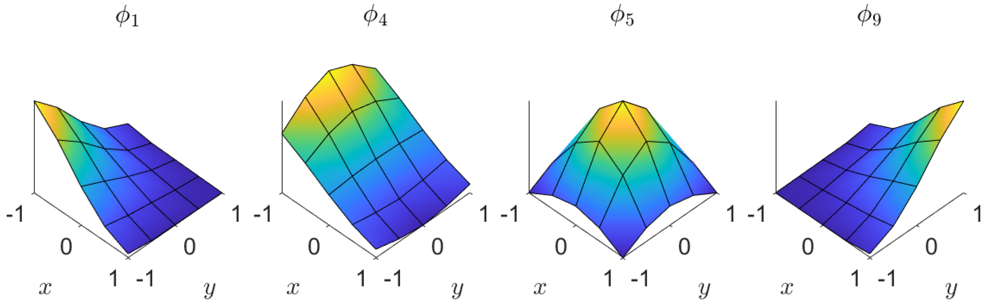
Figure 3.
Shape functions of Figure 2 derived with respect to x.
Figure 3.
Shape functions of Figure 2 derived with respect to x.

Figure 4.
Shape functions of Figure 2 derived with respect to y.
Figure 4.
Shape functions of Figure 2 derived with respect to y.
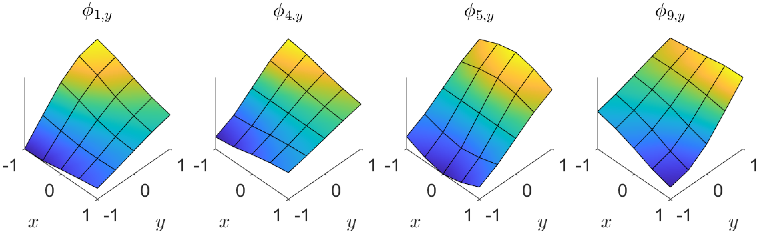
Figure 5.
Convergence analysis results.
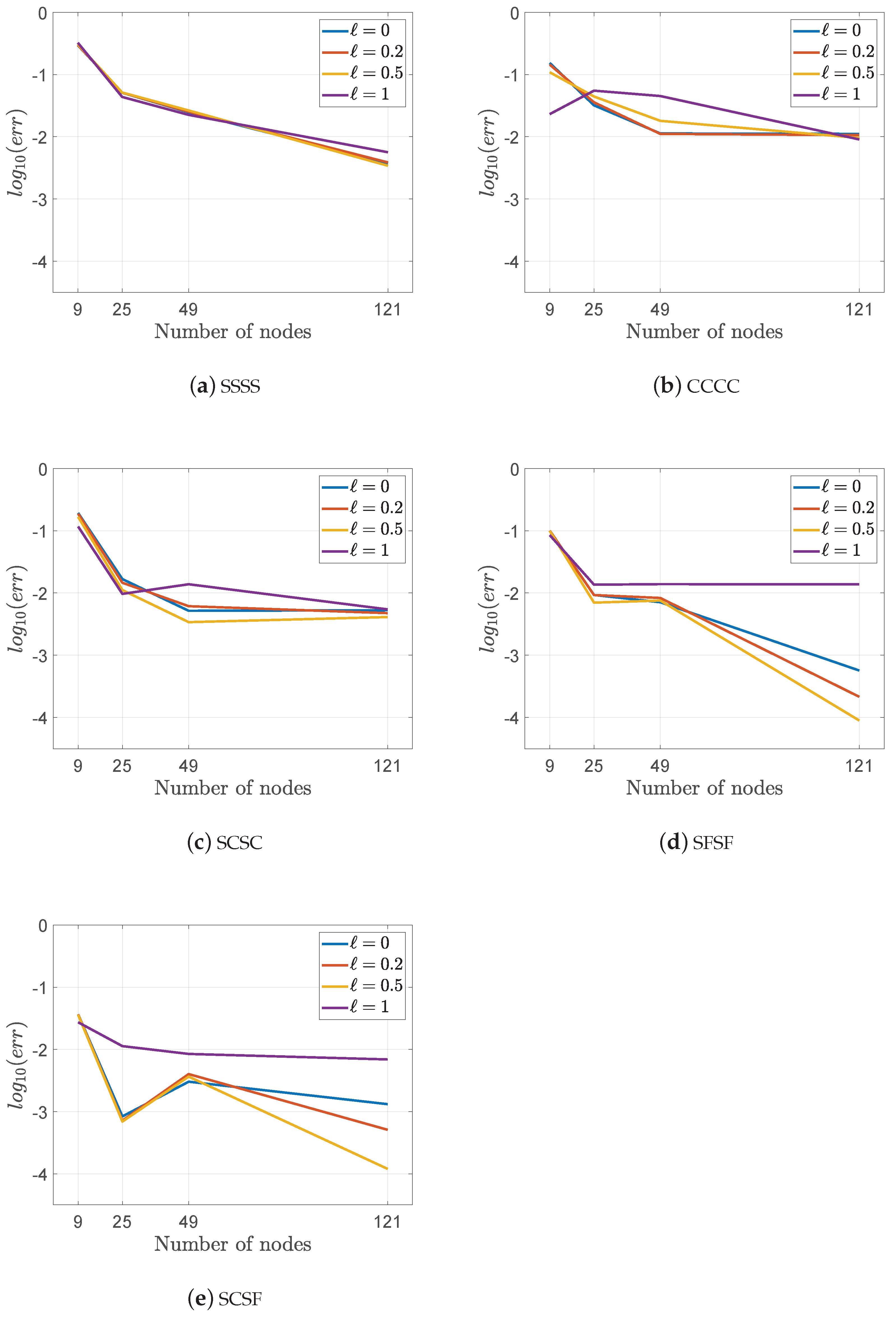
Figure 6.
Deformed shapes of square isotropic nanoplates with different boundary conditions.


Table 1.
Degrees of freedom considered for different kind of materials.
| Material | Degrees of Freedom |
|---|---|
| Isotropic | w |
| Composite | u v w |
Table 2.
Essential boundary conditions considered.
| BCs | ||
|---|---|---|
| Supported | ||
| Clamped | ||
| Free | No variables involved | No variables involved |
Table 3.
Values of for nodal distribution, obtained for , , .
| BC | ℓ (nm) | Exact | Result | Error (%) |
|---|---|---|---|---|
| SSSS | 0 | 4.0624 | 2.8622 | 29.5441 |
| 0.2 | 4.0330 | 2.8338 | 29.7347 | |
| 0.5 | 3.8844 | 2.6956 | 30.6045 | |
| 1 | 3.4231 | 2.3142 | 32.3946 | |
| CCCC | 0 | 1.2653 | 1.0716 | 15.3086 |
| 0.2 | 1.2333 | 1.0555 | 14.4166 | |
| 0.5 | 1.0979 | 0.9785 | 10.8753 | |
| 1 | 0.7946 | 0.7762 | 2.3156 | |
| SCSC | 0 | 1.9171 | 1.5481 | 19.2478 |
| 0.2 | 1.8783 | 1.5269 | 18.7084 | |
| 0.5 | 1.7093 | 1.4247 | 16.6501 | |
| 1 | 1.3040 | 1.1519 | 11.6641 | |
| SFSF | 0 | 15.0113 | 13.5089 | 10.0085 |
| 0.2 | 14.9470 | 13.4511 | 10.0080 | |
| 0.5 | 14.6165 | 13.1711 | 9.8888 | |
| 1 | 13.5451 | 12.3957 | 8.4857 | |
| SCSF | 0 | 11.2359 | 10.8262 | 3.6463 |
| 0.2 | 11.1703 | 10.7635 | 3.6418 | |
| 0.5 | 10.8454 | 10.4568 | 3.5831 | |
| 1 | 9.8416 | 9.5731 | 2.7282 |
Table 4.
Values of for nodal distribution, obtained for , , .
| BC | ℓ (nm) | Exact | Result | Error (%) |
|---|---|---|---|---|
| SSSS | 0 | 4.0624 | 3.8549 | 5.1078 |
| 0.2 | 4.0330 | 3.8262 | 5.1277 | |
| 0.5 | 3.8844 | 3.6844 | 5.1488 | |
| 1 | 3.4231 | 3.2736 | 4.3674 | |
| CCCC | 0 | 1.2653 | 1.3058 | 3.2008 |
| 0.2 | 1.2333 | 1.2774 | 3.5758 | |
| 0.5 | 1.0979 | 1.1466 | 4.4357 | |
| 1 | 0.7946 | 0.8384 | 5.5122 | |
| SCSC | 0 | 1.9171 | 1.8851 | 1.6692 |
| 0.2 | 1.8783 | 1.8509 | 1.4588 | |
| 0.5 | 1.7093 | 1.6903 | 1.1116 | |
| 1 | 1.3040 | 1.2914 | 0.9663 | |
| SFSF | 0 | 15.0113 | 14.8721 | 0.9273 |
| 0.2 | 14.9470 | 14.8087 | 0.9253 | |
| 0.5 | 14.6165 | 14.5144 | 0.6985 | |
| 1 | 13.5451 | 13.7290 | 1.3577 | |
| SCSF | 0 | 11.2359 | 11.2265 | 0.0837 |
| 0.2 | 11.1703 | 11.1623 | 0.0716 | |
| 0.5 | 10.8454 | 10.8529 | 0.0692 | |
| 1 | 9.8416 | 9.9527 | 1.1289 |
Table 5.
Values of for nodal distribution, obtained for , , .
| BC | ℓ (nm) | Exact | Result | Error (%) |
|---|---|---|---|---|
| SSSS | 0 | 4.0624 | 3.9617 | 2.4788 |
| 0.2 | 4.0330 | 3.9310 | 2.5291 | |
| 0.5 | 3.8844 | 3.7815 | 2.6491 | |
| 1 | 3.4231 | 3.3461 | 2.2494 | |
| CCCC | 0 | 1.2653 | 1.2796 | 1.1302 |
| 0.2 | 1.2333 | 1.2470 | 1.1108 | |
| 0.5 | 1.0979 | 1.1177 | 1.8034 | |
| 1 | 0.7946 | 0.8305 | 4.5180 | |
| SCSC | 0 | 1.9171 | 1.9072 | 0.5164 |
| 0.2 | 1.8783 | 1.8668 | 0.6123 | |
| 0.5 | 1.7093 | 1.7035 | 0.3393 | |
| 1 | 1.3040 | 1.3220 | 1.3804 | |
| SFSF | 0 | 15.0113 | 14.9049 | 0.7088 |
| 0.2 | 14.9470 | 14.8228 | 0.8309 | |
| 0.5 | 14.6165 | 14.5063 | 0.7539 | |
| 1 | 13.5451 | 13.7327 | 1.3850 | |
| SCSF | 0 | 11.2359 | 11.2019 | 0.3026 |
| 0.2 | 11.1703 | 11.1255 | 0.4011 | |
| 0.5 | 10.8454 | 10.8058 | 0.3651 | |
| 1 | 9.8416 | 9.9248 | 0.8454 |
Table 6.
Values of for nodal distribution, obtained for , , .
| BC | ℓ (nm) | Exact | Result | Error (%) |
|---|---|---|---|---|
| SSSS | 0 | 4.0624 | 4.0472 | 0.3742 |
| 0.2 | 4.0330 | 4.0174 | 0.3868 | |
| 0.5 | 3.8844 | 3.8711 | 0.3424 | |
| 1 | 3.4231 | 3.4424 | 0.5638 | |
| CCCC | 0 | 1.2653 | 1.2794 | 1.1144 |
| 0.2 | 1.2333 | 1.2464 | 1.0622 | |
| 0.5 | 1.0979 | 1.1084 | 0.9564 | |
| 1 | 0.7946 | 0.8018 | 0.9061 | |
| SCSC | 0 | 1.9171 | 1.9272 | 0.5268 |
| 0.2 | 1.8783 | 1.8872 | 0.4738 | |
| 0.5 | 1.7093 | 1.7163 | 0.4095 | |
| 1 | 1.3040 | 1.3111 | 0.5445 | |
| SFSF | 0 | 15.0113 | 15.0198 | 0.0566 |
| 0.2 | 14.9470 | 14.9430 | 0.0214 | |
| 0.5 | 14.6165 | 14.6178 | 0.0089 | |
| 1 | 13.5451 | 13.7315 | 1.3761 | |
| SCSF | 0 | 11.2359 | 11.2265 | 0.1317 |
| 0.2 | 11.1703 | 11.1623 | 0.0510 | |
| 0.5 | 10.8454 | 10.8529 | 0.0120 | |
| 1 | 9.8416 | 9.9527 | 0.6899 |
Table 7.
Non dimensional values of mid deflection for composite nanoplates, obtained for , , .
| ℓ (nm) | Laminate | Ref. [65] | Result | Error (%) |
|---|---|---|---|---|
| 0 | 0 | 0.004312 | 0.004349 | 0.858071 |
| 0.010636 | 0.010693 | 0.535916 | ||
| 0.005065 | 0.005109 | 0.868707 | ||
| 0.004479 | 0.004520 | 0.915383 | ||
| 0.05 | 0 | 0.002170 | 0.002137 | 1.520737 |
| 0.003931 | 0.004033 | 2.594760 | ||
| 0.002444 | 0.002351 | 3.805237 | ||
| 0.002233 | 0.002167 | 2.955665 | ||
| 0.1 | 0 | 0.001450 | 0.001490 | 2.758621 |
| 0.002522 | 0.002584 | 2.458366 | ||
| 0.001623 | 0.001605 | 1.109057 | ||
| 0.001490 | 0.001497 | 0.469799 |
Publisher’s Note: MDPI stays neutral with regard to jurisdictional claims in published maps and institutional affiliations. |
© 2022 by the authors. Licensee MDPI, Basel, Switzerland. This article is an open access article distributed under the terms and conditions of the Creative Commons Attribution (CC BY) license (https://creativecommons.org/licenses/by/4.0/).
Share and Cite
MDPI and ACS Style
Fabbrocino, F.; Saitta, S.; Vescovini, R.; Fantuzzi, N.; Luciano, R. Meshless Computational Strategy for Higher Order Strain Gradient Plate Models. Math. Comput. Appl. 2022, 27, 19. https://doi.org/10.3390/mca27020019
AMA Style
Fabbrocino F, Saitta S, Vescovini R, Fantuzzi N, Luciano R. Meshless Computational Strategy for Higher Order Strain Gradient Plate Models. Mathematical and Computational Applications. 2022; 27(2):19. https://doi.org/10.3390/mca27020019
Chicago/Turabian StyleFabbrocino, Francesco, Serena Saitta, Riccardo Vescovini, Nicholas Fantuzzi, and Raimondo Luciano. 2022. "Meshless Computational Strategy for Higher Order Strain Gradient Plate Models" Mathematical and Computational Applications 27, no. 2: 19. https://doi.org/10.3390/mca27020019