
The Unit Teissier Distribution and Its Applications


1
Department of Statistics, Cochin University of Science and Technology, Cochin 682022, Kerala, India
2
Department of Statistics, Government College for Women, Trivandrum 695014, Kerala, India
3
Laboratoire de Mathématiques Nicolas Oresme (LMNO), Université de Caen Normandie, Campus II, Science 3, 14032 Caen, France
*
Author to whom correspondence should be addressed.
Math. Comput. Appl. 2022, 27(1), 12; https://doi.org/10.3390/mca27010012
Submission received: 29 December 2021
/
Revised: 25 January 2022
/
Accepted: 29 January 2022
/
Published: 1 February 2022
(This article belongs to the Special Issue Computational Mathematics and Applied Statistics)
Abstract
:A bounded form of the Teissier distribution, namely the unit Teissier distribution, is introduced. It is subjected to a thorough examination of its important properties, including shape analysis of the main functions, analytical expression for moments based on upper incomplete gamma function, incomplete moments, probability-weighted moments, and quantile function. The uncertainty measures Shannon entropy and extropy are also performed. The maximum likelihood estimation, least square estimation, weighted least square estimation, and Bayesian estimation methods are used to estimate the parameters of the model, and their respective performances are assessed via a simulation study. Finally, the competency of the proposed model is illustrated by using two data sets from diverse fields.
Keywords:
Teissier distribution; unit Teissier distribution; Lambert W function; entropy; extropy; simulation; estimationMSC:
60E05; 62F10; 33B301. Introduction
The introduction of new statistical distributions, defined on both the whole real line and the positive real line, is required for the interpretation of real-world occurrences. In both of these lines, a large number of probability distributions for real data sets have been presented recently. Several distributions that fall within these two categories have demonstrated their importance from both a theoretical and practical standpoint. It is true, however, that in many practical disciplines such as economics, medicine, biology, and others, there is a problem of bounded phenomena, or uncertainty resulting from factors such as rates, indices, proportions, and test scores. It is also important to note that, in comparing distributions with unbounded support to those with bounded support, one can find notable scarceness. As a result, in the recent past, some authors have focused on developing distributions that are defined on the bounded interval using any one of the parent distribution transformation techniques. For better understanding, we refer to recent papers in [1,2].
The beta distribution is definitely the most famous distribution among distributions defined in the interval. While the beta distribution is useful for modeling data on the unit interval, many other distributions have been proposed and studied over time. The readers may refer to the Topp–Leone distribution (see [3]), Kumaraswamy distribution (see [4]) and transformed Leipnik distribution (see [5]). However, in recent times, there has been a growing interest by statisticians in proposing distributions defined by the unit interval corresponding to any continuous distribution. The readers may refer to the log-Lindley distribution (see [6]), exponentiated Topp–Leone distribution (see [7]), unit inverse Gaussian distribution (see [8]), unit Lindley distribution (see [9]), unit Weibull distribution (see [10]), unit Burr-III distribution (see [11]), and unit half normal distribution (see [12]), among others. As a result, a lot of contributions are made to the existing literature. This recent leap in the number of research papers devoted to proposing new distributions in the unit interval exhibits their growing relevance. Despite the fact that many distributions have been proposed and studied as alternatives, there is still no agreement on which distribution is preferred.
In this article, a new bounded distribution is introduced by considering the baseline distribution as the Teissier distribution () which was first introduced by the French biologist Georges Teissier in modeling the mortality of domestic animal species as a result of pure aging (see [13]). A continuous random variable Y is said to have the with parameter if its probability density function (pdf) is given by
The cumulative distribution function (cdf) of Y is given by
Despite its importance, the has been overlooked in the statistical literature. Ref. [14] examined the location version of this model and explored a characterization based on life expectancy as part of a demographic study, four decades after it was introduced. In a later study, Muth [15] found that a -derived distribution has a heavier tail than well-known lifetime distributions such as the gamma, lognormal, and Weibull distributions. This distribution was later used by [16] to estimate the lifetime distribution for a German dataset based on used car prices. The and its location version have been forgotten since [16], and no further references appear in the literature until 2008. Ref. [17] showed that as the parameter decreases to zero, the model approaches the classical exponential distribution. The authors of [18] reintroduced this distribution and its scaled version, and studied its important properties using a generalized integro-exponential function [18,19] can be considered as the two-parameter extensions of the .
The study of the has gained momentum in both theoretical and applied perspectives after the work of [19,20,21,22,23] substantiate this claim. Meanwhile, the and its various variants proved their signature compared to other models for various real-life data sets. This is the chief motivation for looking into the defined on the unit interval, so-called the unit Teissier distribution (), and its competency compared to other popular distributions defined on the unit interval. Finally, it can be concluded that it performs well compared to other distributions for the real-life data sets considered here.
As in the case of real-life data sets that vary over positive real lines and possess a bathtub-shaped hazard rate function (hrf), some real-life data sets that are defined on the unit interval also possess a bathtub-shaped hrf. In the former case, there is a tremendous amount of work in the literature on various models, such as [24,25,26]. As far as the latter case is considered, the papers in [8,27] showed that the unit inverse Gaussian and logit slash distributions, respectively, provide a bathtub-shaped hrf. These two distributions are more intricate because of the presence of the log function in their pdfs, and so their cdfs are not obtained in closed form. Hence, simulation experiments from these two distributions are very difficult. For some real data sets, the logit slash distribution does not yield a numerical estimation of parameters. Moreover, the hrfs of both of these distributions are not analytically tractable, even though they sketch the graph of the hrf and provide its various shapes. In addition, Korkmaz [27] proved that the logit slash distribution possesses a N-shaped (modified bathtub shape) and w-shaped bathtub shaped hrf. Another distribution defined on the unit interval, which also possesses a non-monotone shaped hrf, is the unit Modified Burr III distribution (see [28]), which has three parameters. Models with a lower number of parameters are preferable for various reasons, such as ease of simulation drawing and less difficulty in inferential aspects.
The solves these two problems by providing closed form expressions for pdf, cdf, moments, inequality measures, and entropy measures. Secondly, it possesses monotone (increasing and decreasing) as well as non-monotone functions, such as bathtub-shaped and N-shaped hrf (modified bathtub shaped) with a smaller number of parameters. Based on [29], N-shaped hrfs appear in mortality among breast cancer patients.
The rest of the paper is presented as follows. In Section 2, the is introduced and the statistical properties such as moments, incomplete moments, probability-weighted moments, and quantile function are studied. The Shannon entropy and extropy are derived in Section 3. Discussion on different methods of estimation, such as maximum likelihood (ML), ordinary, weighted least square and Bayesian estimation are carried out in Section 4. In Section 5, a simulation study is performed to evaluate the performance of the model parameter estimates. In Section 6, the proposed distribution is elucidated with two real data sets. Finally, the conclusions are presented in Section 7.
2. The Unit Teissier Distribution
In this Section, the is presented and we determine some of its statistical properties.
2.1. Presentation
Mathematically, the is derived from the transformation by taking into account the definition of the pdf given by (1). Its definition is formalized below.
Definition 1.
A random variable X is said to follow the with parameter , if its pdf is of the following form:
The corresponding cdf is given by
2.2. Shapes of the pdf and hrf
As immediate shape properties for the pdf and hrf, we can say that
and that the is unimodal; the mode is the value of x maximizing , which is given by
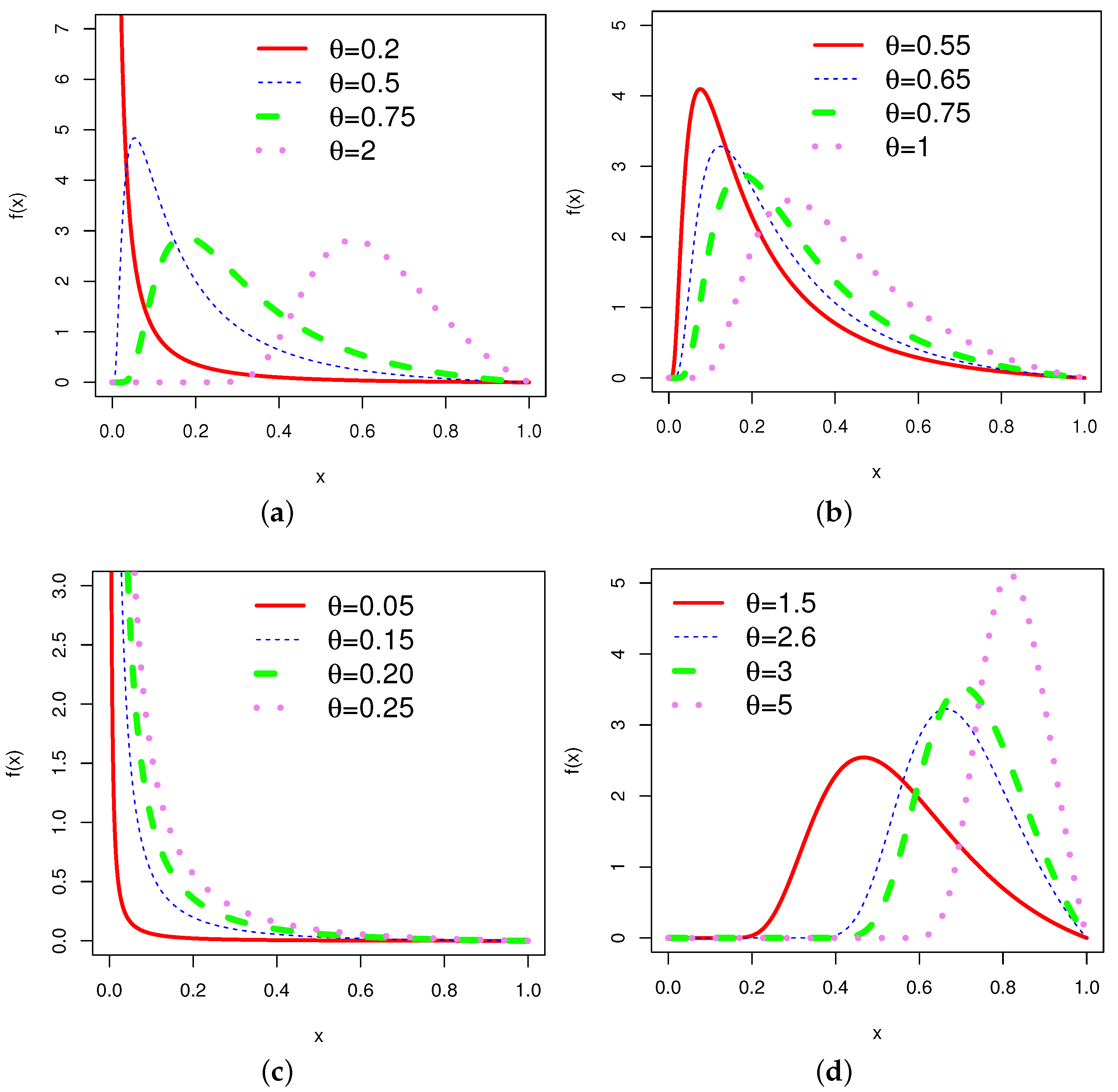
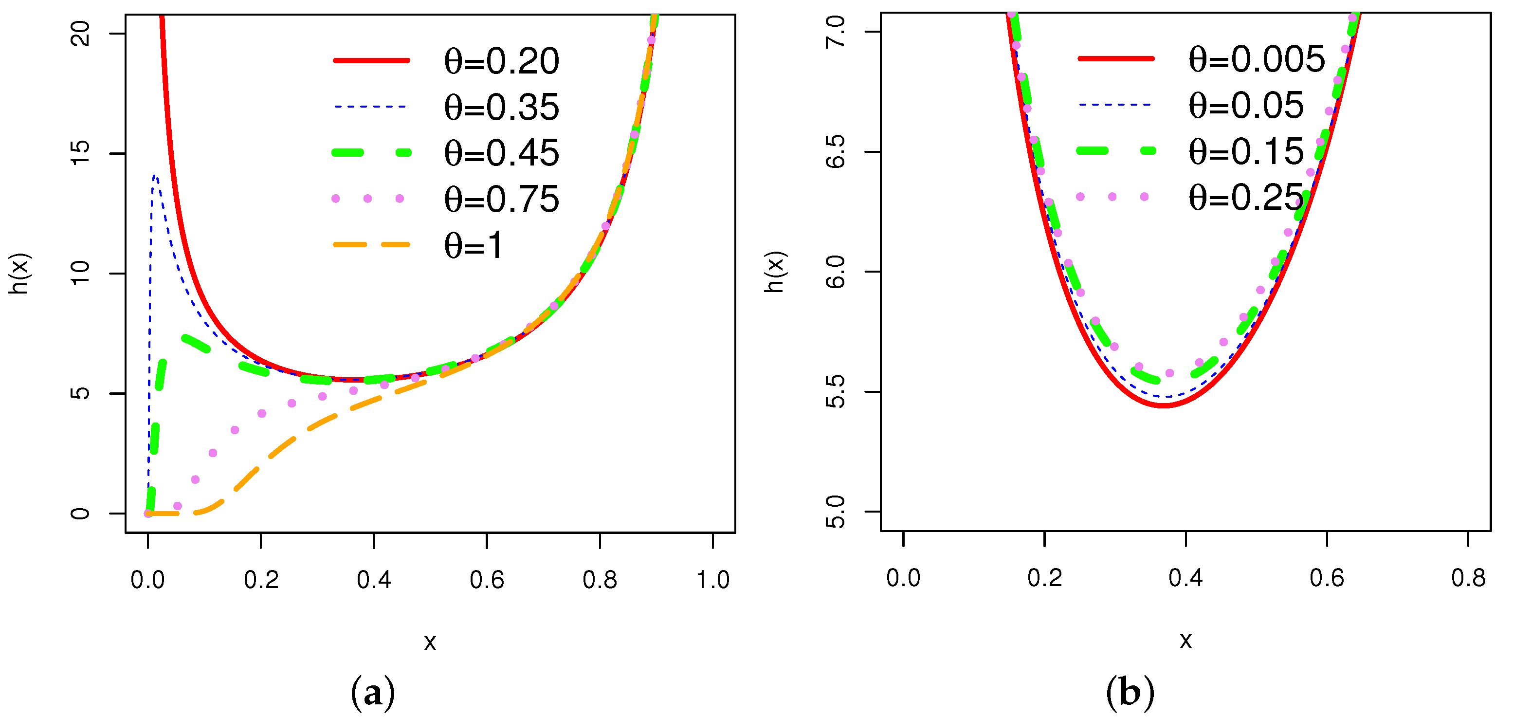
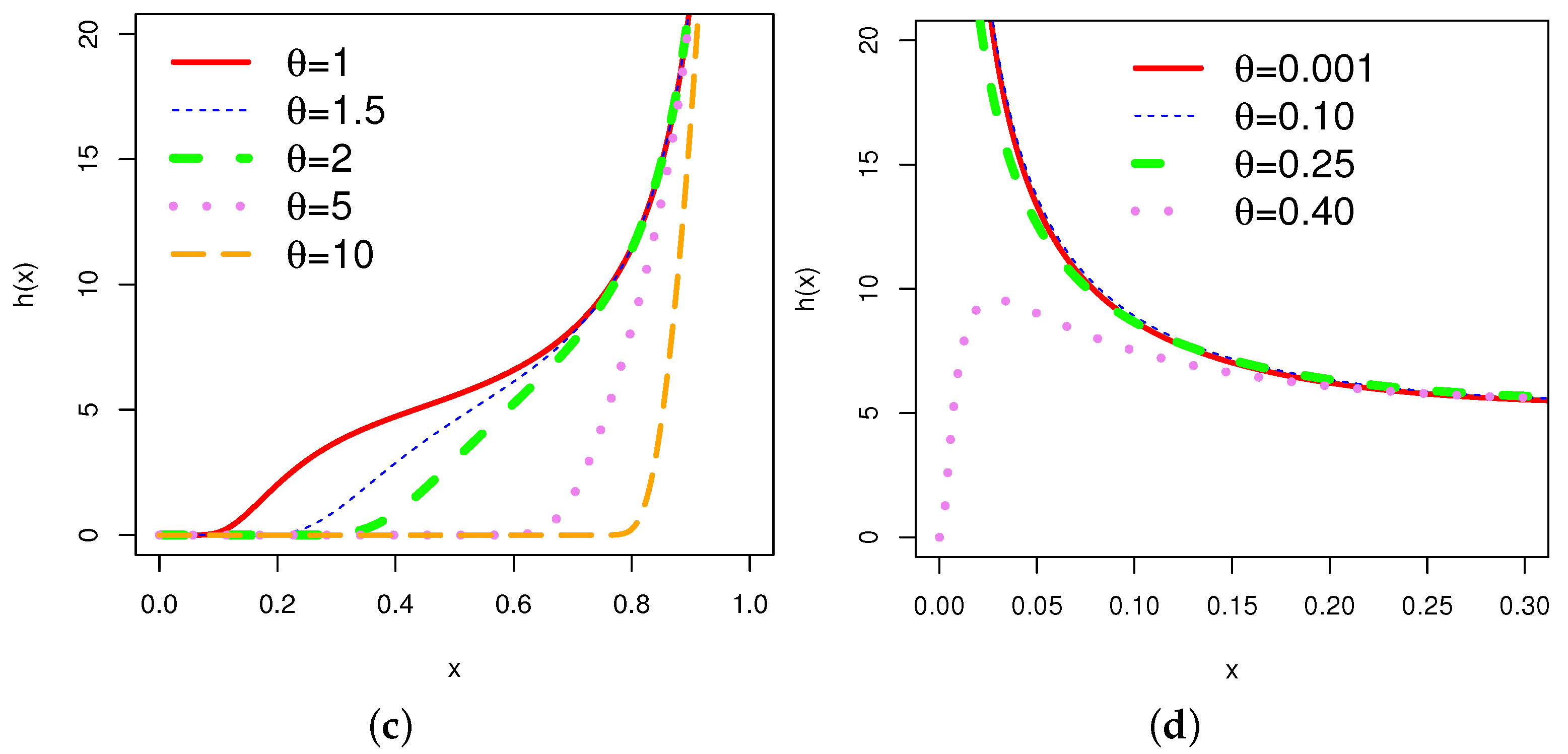
In order to obtain an overview of the shapes of the pdf (2) and hrf (4), the corresponding plots for different choices of the parameter are given in Figure 1 and Figure 2, respectively.
The graphs of the hrf for various combinations of parameters show various shapes, including increasing, decreasing, bathtub, and N-shaped (modified bathtub shape). According to [29], mortality among breast cancer patients is characterized by an N-shaped hrf. This is one of the prominent properties of the .
2.3. Moments
Analytically, the ’s non-central moments can be expressed in terms of the upper incomplete gamma function. This is specified in the result below.
Result 1.
For any non-negative integer r, thenon-central moment of a random variable X with theis
where E denotes the expectation operator,(the exponential function taken at the value 1) andis the upper incomplete gamma function.
Proof.
Based on (2) and the definition of non-central moment, as well as the change of variable , and considering the definition of the upper incomplete gamma function, we have
This ends the proof. □
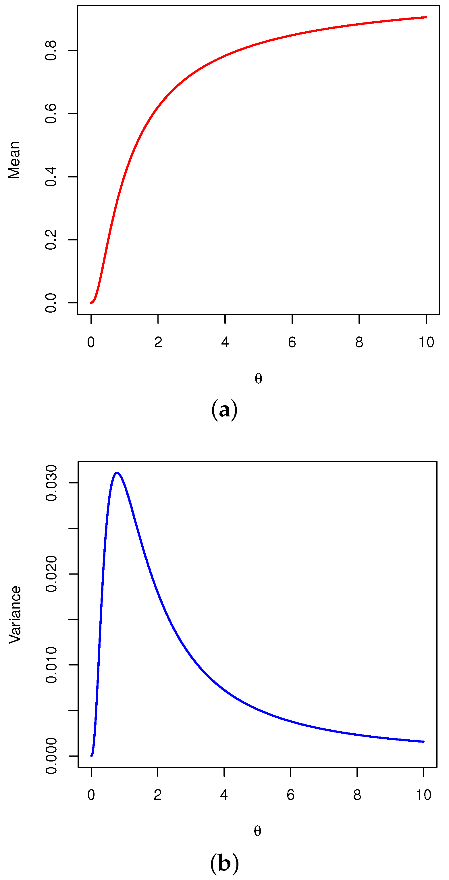
The statistical measures such as the mean () and variance () can be calculated numerically by using R software. Figure 3a,b illustrate the behavior of the mean and variance for varying values of the parameter , respectively.
2.4. Incomplete Moments
As a generalized version of the non-central moments, the ’s incomplete moments can be also expressed in terms of the upper incomplete gamma function.
Result 2.
For any non-negative integer k and, theincomplete moment at x of a random variable X with theis
Proof.
By the definition of the kth incomplete moment, we have
In the above integral expression, after making the change of variable , the proof is similar to the one of Result 1, so the details are excluded here. □
There is an interesting aspect of the fact that the first incomplete moment can be used to compute the mean deviation from the mean () given by .
2.5. Probability-Weighted Moments
The probability-weighted moments of the are now under investigation.
Result 3.
For any non-negative integers r and s, theprobability-weighted moment of a random variable X with theis given as
Proof.
By the definition of the probability-weighted moment and by making the change of variable , we obtain
The desired result is obtained. □
2.6. Mean Residual Life Function
Result 4.
For any, the mean residual life function at t of a random variable X with theis
Proof.
By the definition of the mean residual life function and by making the change of variable , we obtain
The claimed result is achieved. □
2.7. Quantile Function
In addition to its remarkable property of being expressed in closed form, the is also capable of representing the quantile function in terms of the negative branch of the Lambert W function. We recall that the Lambert W function is a multivalued complex function defined as the solution of the equation , where z is a complex number. For any real numbers , has two real branches. The real branch taking on values in is called the principal branch and is denoted by , and the one taking on values in is called the negative branch and is denoted by . For a comprehensive review of this special function, readers are referred to [30]. From a computational perspective, the Lambert W function is available in computer algebra systems such as Maple (function LambertW), Mathematica (function ProductLog), and Matlab (function lambertW), and also in programming languages such as R [31] (functions lambert_W0 and lambert_Wm1 for and , respectively, in the package gsl).
Result 5.
The quantile function of theis given by
whereanddenotes the negative branch of the Lambert W function.
Proof.
The cdf should be inverted to obtain the quantile function of . Thus, we need to solve according to x, so
The obtained x corresponds to the quantile function with respect to p. The desired result is achieved. □
The quantile function in (5) can be used to obtain the following quantities:
- the median given as ;
- the Galton coefficient of skewness specified by
- the Moors coefficient of kurtosis (with correction) defined by
3. Shannon Entropy and Extropy
This section discusses the Shannon entropy and extropy of the .
3.1. Shannon Entropy
Conceptually, the Shannon entropy is the amount of information into a random variable. For a random variable T with pdf with support , its Shannon entropy is defined as
The Shannon entropy for the is obtained in terms of the following quantities:
- The upper incomplete gamma function already introduced;
- The derivative of the gamma function given as ;
- The derivative of the incomplete gamma function given as ;
- The exponential integral defined by
The next result is about the expression of the Shannon entropy.
Result 6.
The Shannon entropy of a random variable T with thehas the following form
3.2. Extropy
Extropy is a complementary dual of Shannon entropy that has a variety of interesting applications, including appropriate scoring of forecasting distributions, comparing the uncertainty of two random variables, and astronomical measurements of heat distributions in galaxies, among others. For a random variable T with pdf with support , its extropy is defined as
Result 7.
The extropy of a random variable T with thehas the following form
4. Estimation and Inference
4.1. Maximum Likelihood Estimation
Let be a random sample of values of size n from a random variable X with the of unknown parameter . Then the likelihood function of is given by
Then the ML estimate (MLE) of , say , is obtained by maximizing with respect to . Thus, for any , we have . Practically, one can use the derivative technique; the partial derivative of with respect to the parameter is
and is obtained by solving the equation according to . Numerical optimization approaches employing mathematical tools such as R and Mathematica are the only way to achieve this.
Fisher Information Matrix and Asymptotic Confidence Interval
In order to carry out statistical inference on the parameters of the , the 1 × 1 expected Fisher information matrix is needed. It can, however, be efficiently approximated by the observed Fisher information matrix given by
and we can approximate variance of as
Then the approximate two-sided normal confidence interval for is given by , where is the upper percentile of a standard normal distribution and is the significance level.
4.2. Ordinary and Weighted Least-Squares Estimation
The ordinary least square (LS) estimation and the weighted least square (WLS) estimation were proposed by [32] to estimate the parameters of the beta distribution. Let be the ordered values of . Let us set
Then the LS estimate (LSE) of , say , is obtained by minimizing with respect to . Thus, for any , we have . Practically, the LSE can also be obtained by solving the following equation:
where
according to . Similarly, the WLS estimate (WLSE) of , say , is obtained by minimizing the non-linear function
and it can also be obtained by solving the following equation:
4.3. Bayesian Estimation
In this subsection, the estimate of the parameter is calculated by using Bayesian analysis. With this approach, prior knowledge about the problem can be incorporated. Here, the parameter should be given a prior density, and two types of priors are used as random priors: the half-Cauchy (HC) and the normal (N) priors. In the numerical integration, prior distributions that are not completely flat provide enough information to allow the numerical approximation algorithm to continue exploring the target posterior density. The HC distribution features such shapes, and its mean and variance do not exist, but its mode is equal to zero. Regarding the HC distribution, when the parameter becomes 25, the pdf is flat, but not entirely. According to [33], depending upon the information necessary, uniform or HC is a better choice of prior. Thus, for the parameter , and are used as prior distributions.
- Case 1:, then the posterior pdf is given by
- Case 2:, then the posterior pdf is given bywhere is derived from (12).
5. Simulation Study
5.1. Simulation for ML, LS, and WLS Estimates
In the simulation study, the Monte Carlo simulation was done in order to prove the efficiency of the model by using different estimation methods such as ML, LS, and WLS. The estimates were calculated for true values of parameters for samples of sizes , and 500 and the following quantities were computed:
- Mean of the estimates: Mean;
- Average bias of the estimates: Bias;
- Mean square error (MSE) of the estimates: MSE
where , and the index i indicates the considered number of the sample. Table 1, Table 2 and Table 3 show the simulation results corresponding to the ML, LS, and WLS estimation methods. A graphical comparison of the MSEs obtained from the three methods is presented in Figure 4. Among these methods, the ML estimation provides accurate estimates of the parameter with the least MSE. As in all the estimation methods, the MSE decreases as sample size n increases, as expected.
5.2. Simulation for Bayesian Estimates
For the parameter , in Section 4.3, the HC distribution (Case 1) and N distribution (Case 2) were motivated as prior distributions. As a result, the posterior summary results, such as means, standard deviations (SDs), Monte Carlo errors (MCEs), lower bounds (LBs), and upper bounds (UBs) of the 95% confidence intervals and medians are summarized in Table 4 and Table 5 for Case 1 and Case 2, respectively. In both cases, increasing sample size leads to a decrease in SD and MCE, which predicts a consistency in the Bayesian estimates.
6. Application
6.1. Methodology
With the help of two real-life data sets, the superiority of the is illustrated. The first data set is from [34]. The data are the maximum flood level (in millions of cubic feet per second) for the Susquehanna River at Harrisburg, Pennsylvania. The second data set represents times between failures of secondary reactor pumps (see [35]).
An analysis of the total time on test (TTT) plot is used to identify the shape of the underlying hrf of the data. We specify that the hrf is decreasing, increasing, bathtub-shaped, and upside-down bathtub-shaped if the empirical TTT transform is convex, concave, convex then concave, and concave then convex, respectively. Thus, it will be shown that the first data set has an increasing hrf, while the second data set has a bathtub-shaped hrf. For the sake of comparison, the following lifetime distributions were considered: Log-Lindley distribution () (see [6]), unit Lindley distribution () (see [9]), Topp–Leone distribution () (see [3]), one-parameter Kumaraswamy distribution (), power distribution (), transmuted distribution (), two-parameter Kumaraswamy distribution (), beta distribution (), exponentiated Topp–Leone distribution (), and unit Burr-III distribution (). Using R software, the MLEs of all these distributions’ parameters are computed along with information criteria, which are listed below.
- Akaike information criterion defined by ;
- Akaike information criterion corrected given as ;
- Consistent Akaike information criterion specified by ;
- Bayesian information criterion defined by
Here, denotes the estimated value of the maximum log-likelihood, p denotes the number of parameters and n denotes the number of observations. The Kolmogorov–Smirnov (KS) test is also used to test the goodness of fit for all the data sets of the and other distributions. Nonparametrically, this test measures how close the empirical distribution and the fitted distribution are. The AIC, AICc, CAIC, and BIC measure the adequacy, while the KS test measures the fit of each distribution. All the computations were performed using R software.
6.2. Flood Level Data
The data set is from [34]. The data represent the maximum flood level (in millions of cubic feet per second) for the Susquehanna River at Harrisburg, Pennsylvania, over 20 four-year periods from 1890 to 1969. Table 6 provides the measurements of the data set.
In Table 7, the MLEs of the parameters of every distribution used and the observed KS test statistics of each distribution are given. We conclude that the gives the best fit because it has the smallest KS value and the largest p-value. Table 8 shows that has the largest maximum log-likelihood value and the smallest AIC, AICc, CAIC, and BIC values among other models. As a result, it can be concluded that the model is more successful than the other models for the flood level data.
Figure 5a,b represent the TTT plot and histogram of flood level data, respectively. The TTT plot indicates an increasing hrf, case covered by the , and histogram depicts how well the proposed model fits the data, compared to other models.
The estimated variance of the MLE of the parameter for the flood level data is given by
Therefore, an approximate 95% confidence interval for is . Table 9 gives the median of bootstrap estimates and bootstrap confidence intervals.
6.3. Times between Failures of Secondary Reactor Pumps Data
The data represent times between failures of secondary reactor pumps (see [35]). Here, a normalization operation is carried out by dividing the original data by 10, in order to obtain data between 0 and 1. Table 10 provides the measurements of the transformed data.
Listed in Table 11 are the MLEs of the parameters and the observed KS test statistic for each distribution. In terms of KS value and p-value, is the best model. On the basis of Table 12, it can be seen that the has the largest log-likelihood value, while the AIC, AICc, CAIC, and BIC values are the smallest. Therefore, the model fits the secondary reactor pump failure data better than the other models.
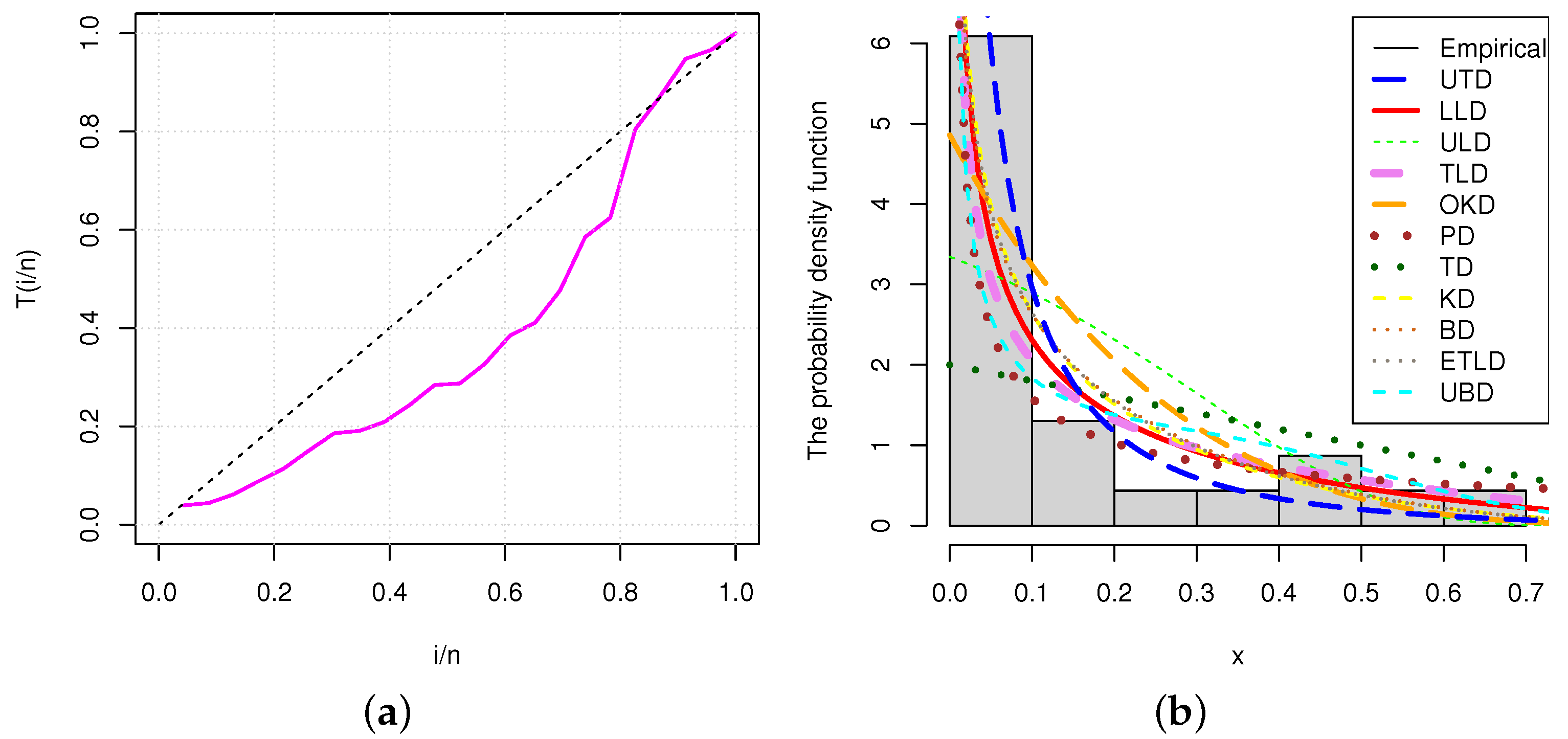
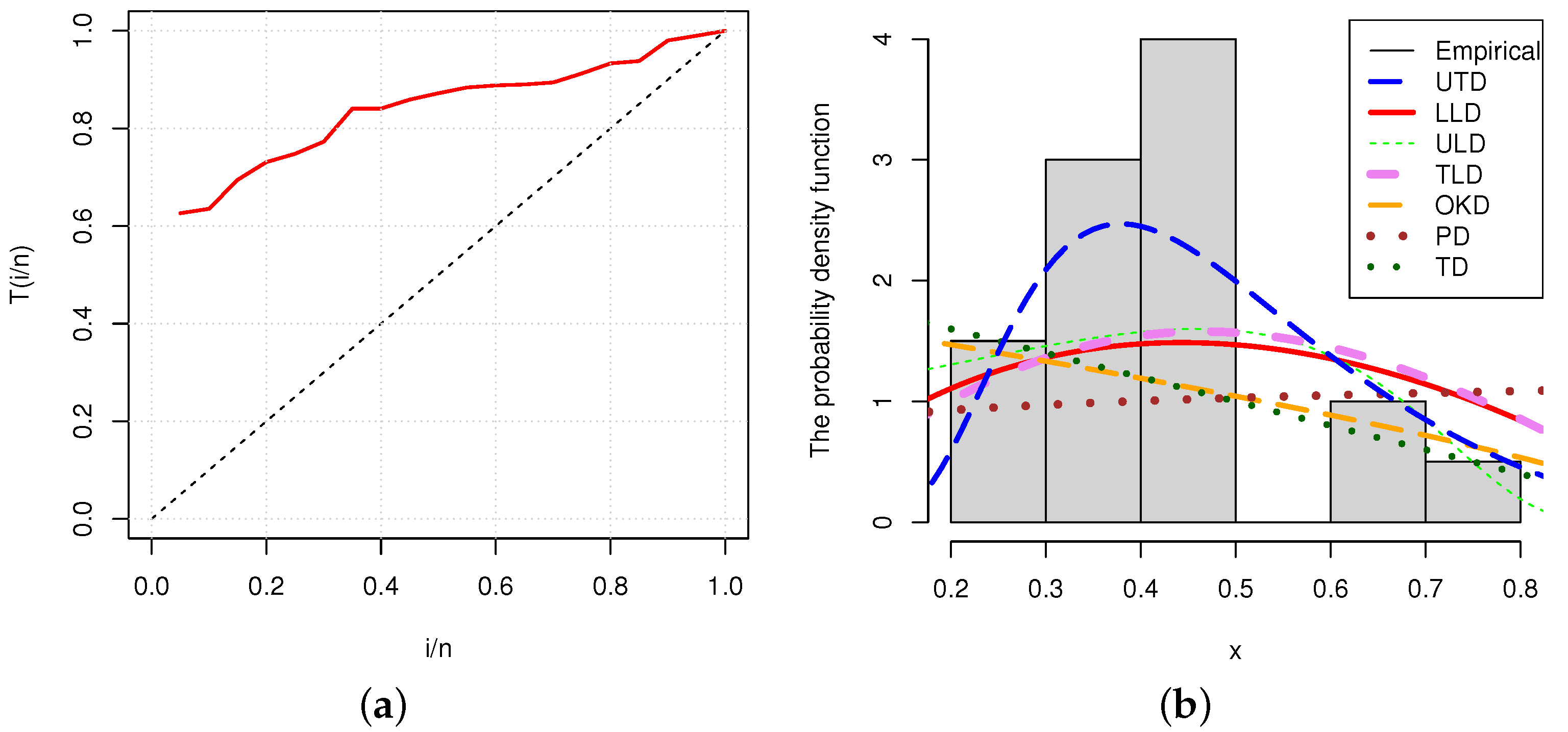
Figure 6a,b represent the empirical TTT plot and histogram of the secondary reactor pumps data. A bathtub hrf is indicated by the TTT plot for the secondary reactor pumps data. From the histogram, it can be seen that the empirical line is closer to the fitted line of the model than other models. The estimated variance of the MLE of the parameter for the times between failures of secondary reactor pumps data data is calculated by
Therefore, an approximate 95% confidence interval for is given by . Table 13 provides the median of bootstrap estimates and bootstrap confidence intervals.
7. Conclusions
Through this study, the introduction of a bounded form of the by the exponential transformation was performed. It is named . Certain statistical properties, such as shape characteristics, moments, incomplete moments, and quantile function were derived. The Shannon entropy and extropy were also obtained. Based on the ML, LS, WLS, and Bayesian methods, estimation of the model parameter was established and examined by simulation studies. The proposed model’s dominance was demonstrated using real-world data sets, and it is concluded that the is a good candidate in unit interval distributions. Possible perspectives of this work include the construction of quantile regression models, as in [36,37], as well as bivariate and discrete versions of the . This work requires additional developments and investigations, which we will leave for future research.
Author Contributions
Conceptualization, A.K., R.M., C.C. and M.R.I.; methodology, A.K., R.M., C.C. and M.R.I.; validation, A.K., R.M., C.C. and M.R.I.; formal analysis, A.K., R.M., C.C. and M.R.I.; investigation, A.K., R.M., C.C. and M.R.I.; writing—original draft preparation, A.K., R.M., C.C. and M.R.I.; writing—review and editing, A.K., R.M., C.C. and M.R.I. All authors have read and agreed to the published version of the manuscript.
Funding
This research received no external funding.
Acknowledgments
We would like to thank the four reviewers for the constructive comments on the paper.
Conflicts of Interest
No potential conflict of interest was reported by the authors.
References
- Lemonte, A.J.; Bazán, J.L. New class of Johnson distributions and its associated regression model for rates and proportions. Biom. J. 2016, 58, 727–746. [Google Scholar] [CrossRef]
- Smithson, M.; Shou, Y. CDF-quantile distributions for modelling random variables on the unit interval. Br. J. Math. Stat. Psychol. 2017, 70, 412–438. [Google Scholar] [CrossRef] [PubMed]
- Topp, C.W.; Leone, F.C. A family of J-shaped frequency functions. J. Am. Stat. Assoc. 1955, 50, 209–219. [Google Scholar] [CrossRef]
- Kumaraswamy, P. A generalized probability density function for double-bounded random processes. J. Hydrol. 1980, 46, 79–88. [Google Scholar] [CrossRef]
- Jorgensen, B. The Theory of Dispersion Models. CRC Monographs on Statistics and Applied Probability; Chapman & Hall: London, UK, 1997. [Google Scholar]
- Gómez-Déniz, E.; Sordo, M.A.; Calderin-Ojeda, E. The Log–Lindley distribution as an alternative to the beta regression model with applications in insurance. Insur. Math. Econ. 2014, 54, 49–57. [Google Scholar] [CrossRef]
- Pourdarvish, A.; Mirmostafaee, S.M.T.K.; Naderi, K. The exponentiated Topp–Leone distribution: Properties and application. J. Appl. Environ. Biol. Sci. 2015, 5, 251–256. [Google Scholar]
- Ghitany, M.E.; Mazucheli, J.; Menezes, A.F.B.; Alqallaf, F. The unit-inverse Gaussian distribution: A new alternative to two-parameter distributions on the unit interval. Commun. Stat. Theory Methods 2019, 48, 3423–3438. [Google Scholar] [CrossRef]
- Mazucheli, J.; Menezes, A.F.B.; Chakraborty, S. On the one parameter unit-Lindley distribution and its associated regression model for proportion data. J. Appl. Stat. 2019, 46, 700–714. [Google Scholar] [CrossRef] [Green Version]
- Mazucheli, J.; Menezes, A.F.B.; Fernandes, L.B.; de Oliveira, R.P.; Ghitany, M.E. The unit-Weibull distribution as an alternative to the Kumaraswamy distribution for the modeling of quantiles conditional on covariates. J. Appl. Stat. 2020, 47, 954–974. [Google Scholar] [CrossRef]
- Modi, K.; Gill, V. Unit Burr-III distribution with application. J. Stat. Manag. Syst. 2020, 23, 579–592. [Google Scholar] [CrossRef]
- Bakouch, H.S.; Nik, A.S.; Asgharzadeh, A.; Salinas, H.S. A flexible probability model for proportion data: Unit-half-normal distribution. Commun. Stat. Case Stud. Data Anal. Appl. 2021, 7, 1–18. [Google Scholar] [CrossRef]
- Teissier, G. Recherches sur le vieillissement et sur les lois de la mortalité. Ann. Physiol. Physicochim. Biol. 1934, 10, 237–284. [Google Scholar]
- Laurent, A.G. Failure and mortality from wear and ageing. The Teissier model. In A Modern Course on Statistical Distributions in Scientific Work; Patil, G.P., Kotz, S., Ord, J.K., Eds.; ASIC; Springer: Berlin/Heidelberg, Germany, 1975; Volume 17, pp. 301–320. [Google Scholar]
- Muth, E.J. Reliability models with positive memory derived from the mean residual life function. Theory Appl. Reliab. 1977, 2, 401–436. [Google Scholar]
- Rinne, H. Estimating the lifetime distribution of private motor-cars using prices of used cars: The Teissier model. In Statistiks Zwischen Theorie und Praxis; Vandenhoeck & Ruprecht: Göttingen, Germany, 1985; pp. 172–184. [Google Scholar]
- Leemis, L.M.; McQueston, J.T. Univariate distribution relationships. Am. Stat. 2008, 62, 45–53. [Google Scholar] [CrossRef]
- Jodrá, P.; Jiménez-Gamero, M.D.; Alba-Fernandez, M.V. On the Muth distribution. Math. Model. Anal. 2015, 20, 291–310. [Google Scholar] [CrossRef]
- Jodrá, P.; Gómez, H.W.; Jiménez-Gamero, M.D.; Alba-Fernández, M.V. The power Muth distribution. Math. Model. Anal. 2017, 22, 186–201. [Google Scholar] [CrossRef]
- Al-Babtain, A.A.; Elbatal, I.; Chesneau, C.; Jamal, F. The transmuted Muth generated class of distributions with applications. Symmetry 2020, 12, 1677. [Google Scholar] [CrossRef]
- Biçer, C.; Bakouch, H.S.; Biçer, H.D. Inference on parameters of a geometric process with scaled Muth distribution. Fluct. Noise Lett. 2021, 20, 2150006. [Google Scholar] [CrossRef]
- Irshad, M.R.; Maya, R.; Arun, S.P. Muth distribution and estimation of a parameter using order statistics. Statistica 2021, 81, 93–119. [Google Scholar]
- Irshad, M.R.; Maya, R.; Krishna, A. Exponentiated power Muth distribution and associated inference. J. Indian Soc. Probab. Stat. 2021, 22, 265–302. [Google Scholar] [CrossRef]
- Abd EL-Baset, A.A.; Ghazal, M.G.M. Exponentiated additive Weibull distribution. Reliab. Eng. Syst. Saf. 2020, 193, 106663. [Google Scholar]
- Alamgir Khalil, M.I.; Ali, K.; Mashwani, W.K.; Shafiq, M.; Kumam, P.; Kumam, W. A novel flexible additive Weibull distribution with real-life applications. Commun. Stat. Theory Methods 2021, 50, 1557–1572. [Google Scholar] [CrossRef]
- Irshad, M.R.; Shibu, D.S.; Maya, R.; D’cruz, V. Binominal mixture Lindley distribution: Properties and Applications. J. Indian Soc. Probab. Stat. 2020, 21, 437–469. [Google Scholar] [CrossRef]
- Korkmaz, M.Ç. A new heavy-tailed distribution defined on the bounded interval: The logit slash distribution and its application. J. Appl. Stat. 2020, 47, 2097–2119. [Google Scholar] [CrossRef]
- Haq, M.A.U.; Hashmi, S.; Aidi, K.; Ramos, P.L.; Louzada, F. Unit modified Burr-III distribution: Estimation, characterizations and validation test. Ann. Data Sci. 2020, 1–26. [Google Scholar] [CrossRef]
- Bebbington, M.; Lai, C.D.; Murthy, D.N.P.; Zitikis, R. Modelling N-and W-shaped hazard rate functions without mixing distributions. Proc. Inst. Mech. Eng. Part O J. Risk Reliab. 2009, 223, 59–69. [Google Scholar] [CrossRef]
- Corless, R.M.; Gonnet, G.H.; Hare, D.E.G.; Jeffrey, D.J.; Knuth, D.E. On the Lambert W function. Adv. Comput. Math. 1996, 5, 329–359. [Google Scholar] [CrossRef]
- R Development Core Team. R: A Language and Environment for Statistical Computing; R Foundation for Statistical Computing: Vienna, Austria, 2021; Available online: http://www.R-project.org/ (accessed on 28 December 2021).
- Swain, J.J.; Venkatraman, S.; Wilson, J.R. Least-squares estimation of distribution functions in Johnson’s translation system. J. Stat. Comput. Simul. 1988, 29, 271–297. [Google Scholar] [CrossRef]
- Gelman, A.; Hill, J. Data Analysis Using Regression and Multilevel/Hierarchical Models; Cambridge University Press: Cambridge, UK, 2006. [Google Scholar]
- Dumonceaux, R.; Antle, C.E. Discrimination between the log-normal and the Weibull distributions. Technometrics 1973, 15, 923–926. [Google Scholar] [CrossRef]
- Suprawhardana, M.S.; Prayoto, S. Total time on test plot analysis for mechanical components of the RSG-GAS reactor. At. Indones. 1999, 25, 81–90. [Google Scholar]
- Korkmaz, M.Ç.; Chesneau, C.; Korkmaz, Z.S. On the arcsecant hyperbolic normal distribution. Properties, quantile regression modeling and applications. Symmetry 2021, 13, 117. [Google Scholar] [CrossRef]
- Korkmaz, M.Ç.; Chesneau, C. On the unit Burr-XII distribution with the quantile regression modeling and applications. Comput. Appl. Math. 2021, 40, 29. [Google Scholar] [CrossRef]
Figure 1.
Plots of various shapes of the pdf of the for varying values of the parameter .

Figure 2.
Plots of various shapes of the hrf of the for varying values of the parameter .


Figure 3.
Plots of the (a) mean and (b) variance of the for varying values of the parameter .

Figure 4.
Graphical comparison of the MSEs obtained from ML, LS, and WLS estimation methods for (a) , (b) , (c) , (d) , (e) and (f) .
Figure 4.
Graphical comparison of the MSEs obtained from ML, LS, and WLS estimation methods for (a) , (b) , (c) , (d) , (e) and (f) .
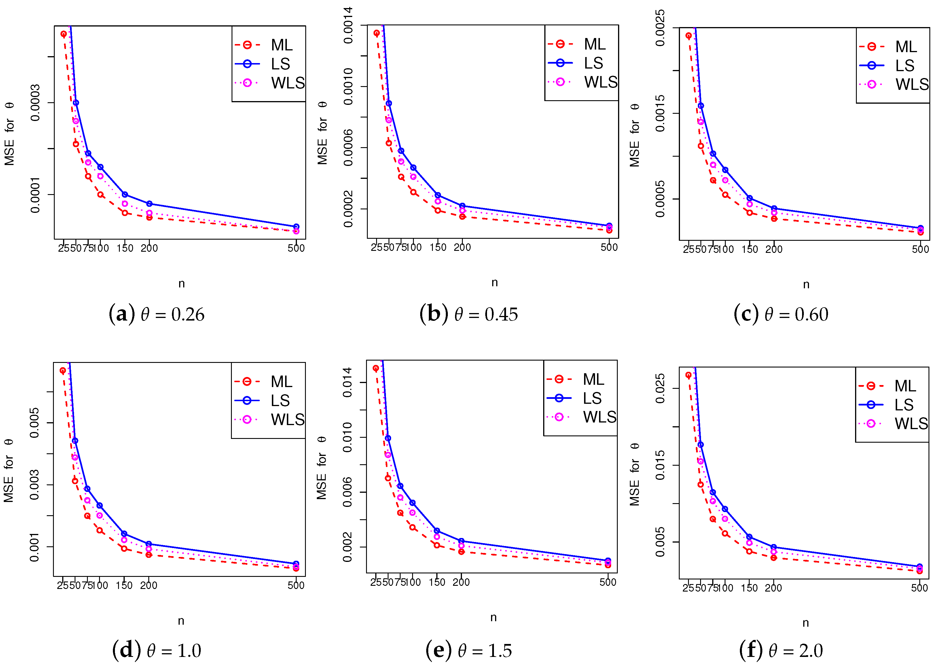
Figure 5.
(a) TTT plot and (b) histogram for the flood level data.

Figure 6.
(a) TTT plot and (b) histogram for secondary reactor pumps data.

Table 1.
Simulation results: MLEs, bias, and MSE.
| n | Bias() | MSE() | Bias() | MSE() | Bias() | MSE() | |||
| 25 | 0.26352 | 0.00352 | 0.00045 | 0.45610 | 0.00610 | 0.00135 | 0.60813 | 0.00813 | 0.00241 |
| 50 | 0.26164 | 0.00164 | 0.00021 | 0.45284 | 0.00284 | 0.00063 | 0.60379 | 0.00379 | 0.00112 |
| 75 | 0.26116 | 0.00116 | 0.00014 | 0.45200 | 0.00200 | 0.00041 | 0.60267 | 0.00267 | 0.00072 |
| 100 | 0.26074 | 0.00074 | 0.00010 | 0.45129 | 0.00129 | 0.00031 | 0.60172 | 0.00172 | 0.00055 |
| 150 | 0.26042 | 0.00042 | 0.00006 | 0.45074 | 0.00074 | 0.00019 | 0.60098 | 0.00098 | 0.00034 |
| 200 | 0.26028 | 0.00028 | 0.00005 | 0.45049 | 0.00049 | 0.00015 | 0.60065 | 0.00065 | 0.00027 |
| 500 | 0.26011 | 0.00011 | 0.00002 | 0.45019 | 0.00019 | 0.00006 | 0.60025 | 0.00025 | 0.00011 |
| n | Bias() | MSE() | Bias() | MSE() | Bias() | MSE() | |||
| 25 | 1.01355 | 0.01355 | 0.00669 | 1.52033 | 0.02033 | 0.01505 | 2.02711 | 0.02711 | 0.02676 |
| 50 | 1.00632 | 0.00632 | 0.00312 | 1.50948 | 0.00948 | 0.00702 | 2.01264 | 0.01264 | 0.01248 |
| 75 | 1.00446 | 0.00446 | 0.00200 | 1.50668 | 0.00668 | 0.00450 | 2.00891 | 0.00891 | 0.00800 |
| 100 | 1.00286 | 0.00286 | 0.00153 | 1.50429 | 0.00429 | 0.00344 | 2.00572 | 0.00572 | 0.00612 |
| 150 | 1.00163 | 0.00163 | 0.00094 | 1.50245 | 0.00245 | 0.00213 | 2.00327 | 0.00327 | 0.00378 |
| 200 | 1.00109 | 0.00109 | 0.00074 | 1.50164 | 0.00164 | 0.00166 | 2.00218 | 0.00218 | 0.00295 |
| 500 | 1.00041 | 0.00041 | 0.00030 | 1.50062 | 0.00062 | 0.00068 | 2.00082 | 0.00082 | 0.00121 |
Table 2.
Simulation results: LS estimates, bias, and MSE.
| n | Bias() | MSE() | Bias() | MSE() | Bias() | MSE() | |||
| 25 | 0.26122 | 0.00122 | 0.00069 | 0.45210 | 0.00210 | 0.00207 | 0.60280 | 0.00280 | 0.00368 |
| 50 | 0.25998 | −0.00002 | 0.00030 | 0.44997 | −0.00003 | 0.00089 | 0.59996 | −0.00004 | 0.00159 |
| 75 | 0.25997 | −0.00003 | 0.00019 | 0.44994 | −0.00006 | 0.00058 | 0.59992 | −0.00008 | 0.00103 |
| 100 | 0.25990 | −0.00010 | 0.00016 | 0.44983 | −0.00017 | 0.00047 | 0.59977 | −0.00023 | 0.00084 |
| 150 | 0.25954 | −0.00046 | 0.00010 | 0.44920 | −0.00080 | 0.00029 | 0.59893 | −0.00107 | 0.00051 |
| 200 | 0.26057 | 0.00057 | 0.00008 | 0.44914 | −0.00086 | 0.00022 | 0.59886 | −0.00114 | 0.00039 |
| 500 | 0.25980 | −0.00020 | 0.00003 | 0.44964 | −0.00036 | 0.00009 | 0.59953 | −0.00047 | 0.00016 |
| n | Bias() | MSE() | Bias() | MSE() | Bias() | MSE() | |||
| 25 | 1.00467 | 0.00467 | 0.01021 | 1.50701 | 0.00701 | 0.02297 | 2.00935 | 0.00935 | 0.04083 |
| 50 | 0.99993 | −0.00007 | 0.00442 | 1.49990 | −0.00010 | 0.00994 | 1.99986 | −0.00014 | 0.01768 |
| 75 | 0.99986 | −0.00014 | 0.00287 | 1.49979 | −0.00021 | 0.00646 | 1.99972 | −0.00028 | 0.01148 |
| 100 | 0.99961 | −0.00039 | 0.00233 | 1.49942 | −0.00058 | 0.00523 | 1.99923 | −0.00077 | 0.00930 |
| 150 | 0.99821 | −0.00179 | 0.00142 | 1.49732 | −0.00268 | 0.00319 | 1.99643 | −0.00357 | 0.00567 |
| 200 | 0.99809 | −0.00191 | 0.00109 | 1.49714 | −0.00286 | 0.00244 | 1.99619 | −0.00381 | 0.00434 |
| 500 | 0.99921 | −0.00079 | 0.00045 | 1.49881 | −0.00119 | 0.00101 | 1.99842 | −0.00158 | 0.00180 |
Table 3.
Simulation results: WLS estimates, bias, and MSE.
| n | Bias() | MSE() | Bias() | MSE() | Bias() | MSE() | |||
| 25 | 0.26141 | 0.00141 | 0.00062 | 0.45243 | 0.00243 | 0.00186 | 0.60324 | 0.00324 | 0.00330 |
| 50 | 0.26024 | 0.00024 | 0.00026 | 0.45041 | 0.00041 | 0.00078 | 0.60055 | 0.00055 | 0.00140 |
| 75 | 0.26018 | 0.00018 | 0.00017 | 0.45030 | 0.00030 | 0.00051 | 0.60041 | 0.00041 | 0.00090 |
| 100 | 0.26007 | 0.00007 | 0.00014 | 0.45012 | 0.00012 | 0.00041 | 0.60016 | 0.00016 | 0.00072 |
| 150 | 0.25971 | −0.00029 | 0.00008 | 0.44950 | −0.00050 | 0.00025 | 0.59934 | −0.00066 | 0.00044 |
| 200 | 0.25968 | −0.00032 | 0.00006 | 0.44944 | −0.00056 | 0.00019 | 0.59925 | −0.00075 | 0.00034 |
| 500 | 0.25986 | 0.00014 | 0.00001 | 0.44976 | −0.00024 | 0.00008 | 0.59968 | −0.00032 | 0.00014 |
| n | Bias() | MSE() | Bias() | MSE() | Bias() | MSE() | |||
| 25 | 1.00540 | 0.00540 | 0.00917 | 1.50809 | 0.00809 | 0.02063 | 2.01079 | 0.01079 | 0.03668 |
| 50 | 1.00091 | 0.00091 | 0.00388 | 1.50137 | 0.00137 | 0.00872 | 2.00182 | 0.00182 | 0.01550 |
| 75 | 1.00067 | 0.00067 | 0.00250 | 1.50101 | 0.00101 | 0.00562 | 2.00135 | 0.00135 | 0.00999 |
| 100 | 1.00026 | 0.00026 | 0.00201 | 1.50039 | 0.00039 | 0.00451 | 2.00052 | 0.00052 | 0.00802 |
| 150 | 0.99889 | −0.00111 | 0.00122 | 1.49834 | −0.00166 | 0.00275 | 1.99778 | −0.00222 | 0.00490 |
| 200 | 0.99876 | −0.00124 | 0.00093 | 1.49813 | −0.00187 | 0.00210 | 1.99751 | −0.00249 | 0.00373 |
| 500 | 0.99946 | −0.00054 | 0.00038 | 1.49919 | −0.00081 | 0.00087 | 1.99892 | −0.00108 | 0.00154 |
Table 4.
Posterior summary results (Case 1: ).
| n | Mean | SD | MCE | LB | UB | Median |
| 25 | 0.26217 | 0.01971 | 0.00300 | 0.22331 | 0.28030 | 0.26770 |
| 50 | 0.26834 | 0.01649 | 0.00213 | 0.24361 | 0.29064 | 0.26831 |
| 75 | 0.27247 | 0.01599 | 0.00206 | 0.25154 | 0.29064 | 0.27118 |
| 100 | 0.26770 | 0.01057 | 0.00175 | 0.25917 | 0.28695 | 0.26957 |
| 150 | 0.27098 | 0.00938 | 0.00154 | 0.25339 | 0.28218 | 0.26928 |
| 200 | 0.26300 | 0.00638 | 0.00123 | 0.25714 | 0.26781 | 0.26407 |
| 500 | 0.27236 | 0.00264 | 0.00109 | 0.26706 | 0.27597 | 0.27425 |
| n | Mean | SD | MCE | LB | UB | Median |
| 25 | 0.45493 | 0.04530 | 0.00889 | 0.36841 | 0.52298 | 0.45676 |
| 50 | 0.47560 | 0.02125 | 0.00716 | 0.43660 | 0.51318 | 0.46884 |
| 75 | 0.46305 | 0.02069 | 0.00598 | 0.41964 | 0.50306 | 0.46555 |
| 100 | 0.47071 | 0.01648 | 0.00517 | 0.42378 | 0.49429 | 0.47592 |
| 150 | 0.46769 | 0.01489 | 0.00393 | 0.42507 | 0.49429 | 0.46646 |
| 200 | 0.45651 | 0.00991 | 0.00262 | 0.44271 | 0.47886 | 0.45687 |
| 500 | 0.46907 | 0.00830 | 0.00231 | 0.44839 | 0.48607 | 0.46841 |
| n | Mean | SD | MCE | LB | UB | Median |
| 25 | 0.62836 | 0.05583 | 0.01269 | 0.51515 | 0.69347 | 0.65291 |
| 50 | 0.63488 | 0.03203 | 0.00815 | 0.55716 | 0.68275 | 0.63661 |
| 75 | 0.63130 | 0.02958 | 0.00740 | 0.54930 | 0.68275 | 0.63682 |
| 100 | 0.64362 | 0.02506 | 0.00657 | 0.59327 | 0.68275 | 0.65125 |
| 150 | 0.61670 | 0.02001 | 0.00473 | 0.59286 | 0.65175 | 0.60516 |
| 200 | 0.58433 | 0.01135 | 0.00361 | 0.56540 | 0.60849 | 0.58477 |
| 500 | 0.61527 | 0.00864 | 0.00333 | 0.60791 | 0.63575 | 0.61179 |
| n | Mean | SD | MCE | LB | UB | Median |
| 25 | 1.02150 | 0.08400 | 0.01689 | 0.84895 | 1.13786 | 1.02060 |
| 50 | 1.02859 | 0.08394 | 0.01243 | 0.94449 | 1.15295 | 1.02883 |
| 75 | 1.04385 | 0.04133 | 0.01163 | 0.92371 | 1.09369 | 1.04292 |
| 100 | 1.06278 | 0.04029 | 0.01001 | 1.02172 | 1.22162 | 1.05589 |
| 150 | 1.03099 | 0.03427 | 0.00846 | 0.98819 | 1.07907 | 1.03083 |
| 200 | 1.02172 | 0.02549 | 0.00573 | 0.99575 | 1.05466 | 1.02620 |
| 500 | 0.97150 | 0.01249 | 0.00484 | 0.94968 | 0.98967 | 0.97079 |
| n | Mean | SD | MCE | LB | UB | Median |
| 25 | 1.52918 | 0.14300 | 0.04025 | 1.31918 | 1.78305 | 1.50069 |
| 50 | 1.51870 | 0.11159 | 0.03641 | 1.17142 | 1.67897 | 1.55316 |
| 75 | 1.40491 | 0.09922 | 0.03165 | 1.20423 | 1.52690 | 1.42708 |
| 100 | 1.56450 | 0.07915 | 0.02093 | 1.25097 | 1.64389 | 1.57598 |
| 150 | 1.54486 | 0.05005 | 0.01196 | 1.47530 | 1.61097 | 1.55532 |
| 200 | 1.52040 | 0.02288 | 0.00591 | 1.50104 | 1.56919 | 1.52027 |
| 500 | 1.55005 | 0.02201 | 0.00390 | 1.52843 | 1.58571 | 1.55540 |
| n | Mean | SD | MCE | LB | UB | Median |
| 25 | 2.06736 | 0.15240 | 0.03757 | 1.74925 | 2.30008 | 2.13126 |
| 50 | 2.07023 | 0.14915 | 0.02789 | 1.75671 | 2.29423 | 2.09929 |
| 75 | 2.07862 | 0.11586 | 0.02615 | 1.92777 | 2.22704 | 2.06513 |
| 100 | 2.09001 | 0.07422 | 0.02596 | 1.99647 | 2.20813 | 2.07646 |
| 150 | 2.03891 | 0.07322 | 0.02149 | 1.75963 | 2.14525 | 2.06189 |
| 200 | 2.06265 | 0.05250 | 0.01654 | 1.99405 | 2.26134 | 2.05505 |
| 500 | 2.09538 | 0.04211 | 0.01636 | 2.06500 | 2.21627 | 2.06596 |
Table 5.
Posterior summary results (Case 2: ).
| n | Mean | SD | MCE | LB | UB | Median |
| 25 | 0.25141 | 0.05134 | 0.01312 | 0.04355 | 0.30548 | 0.26122 |
| 50 | 0.25790 | 0.04318 | 0.01151 | 0.15933 | 0.29794 | 0.26140 |
| 75 | 0.26324 | 0.03247 | 0.00592 | 0.24319 | 0.28917 | 0.26559 |
| 100 | 0.27617 | 0.01091 | 0.00322 | 0.25228 | 0.29550 | 0.27556 |
| 150 | 0.24699 | 0.01081 | 0.00208 | 0.23512 | 0.26737 | 0.24183 |
| 200 | 0.26654 | 0.01409 | 0.00285 | 0.25307 | 0.30800 | 0.26631 |
| 500 | 0.26818 | 0.01401 | 0.00159 | 0.26320 | 0.28228 | 0.26949 |
| n | Mean | SD | MCE | LB | UB | Median |
| 25 | 0.44924 | 0.04779 | 0.01029 | 0.37730 | 0.52804 | 0.44985 |
| 50 | 0.46277 | 0.03141 | 0.00797 | 0.41231 | 0.51942 | 0.46657 |
| 75 | 0.46092 | 0.02074 | 0.00545 | 0.41995 | 0.49405 | 0.45864 |
| 100 | 0.47382 | 0.01515 | 0.00498 | 0.44194 | 0.50921 | 0.47630 |
| 150 | 0.43418 | 0.01103 | 0.00326 | 0.41547 | 0.44902 | 0.43349 |
| 200 | 0.46069 | 0.01011 | 0.00263 | 0.44098 | 0.48238 | 0.46259 |
| 500 | 0.46553 | 0.00599 | 0.00182 | 0.45494 | 0.47738 | 0.46694 |
| n | Mean | SD | MCE | LB | UB | Median |
| 25 | 0.60442 | 0.05548 | 0.01444 | 0.49541 | 0.71972 | 0.60913 |
| 50 | 0.54888 | 0.03104 | 0.01281 | 0.49527 | 0.62074 | 0.55447 |
| 75 | 0.61557 | 0.02836 | 0.00759 | 0.57167 | 0.65640 | 0.61174 |
| 100 | 0.62561 | 0.01481 | 0.00538 | 0.60462 | 0.65368 | 0.62487 |
| 150 | 0.58561 | 0.01322 | 0.00402 | 0.55367 | 0.60185 | 0.58913 |
| 200 | 0.59753 | 0.01138 | 0.00449 | 0.58214 | 0.61691 | 0.59483 |
| 500 | 0.61042 | 0.01113 | 0.00361 | 0.59462 | 0.63647 | 0.61434 |
| n | Mean | SD | MCE | LB | UB | Median |
| 25 | 1.02150 | 0.08400 | 0.01689 | 0.84895 | 1.13786 | 1.02060 |
| 50 | 1.03794 | 0.06691 | 0.01658 | 0.89983 | 1.14142 | 1.04985 |
| 75 | 1.04394 | 0.05572 | 0.01330 | 0.90487 | 1.14142 | 1.04432 |
| 100 | 1.04440 | 0.04849 | 0.01302 | 0.92824 | 1.14142 | 1.03943 |
| 150 | 1.05009 | 0.04125 | 0.01278 | 0.98320 | 1.13767 | 1.05431 |
| 200 | 1.00869 | 0.07225 | 0.01869 | 0.90478 | 1.07876 | 1.01865 |
| 500 | 1.01614 | 0.06391 | 0.00458 | 1.00317 | 1.04602 | 1.01625 |
| n | Mean | SD | MCE | LB | UB | Median |
| 25 | 1.52918 | 0.14300 | 0.04025 | 1.31918 | 1.78305 | 1.50069 |
| 50 | 1.54627 | 0.07872 | 0.02170 | 1.38232 | 1.64742 | 1.55280 |
| 75 | 1.55881 | 0.06692 | 0.01959 | 1.44383 | 1.66958 | 1.55559 |
| 100 | 1.55876 | 0.04834 | 0.01311 | 1.45950 | 1.62751 | 1.55994 |
| 150 | 1.55805 | 0.03772 | 0.01221 | 1.48935 | 1.63206 | 1.55871 |
| 200 | 1.52328 | 0.10483 | 0.00849 | 1.45942 | 1.66891 | 1.52085 |
| 500 | 1.53107 | 0.09938 | 0.00683 | 1.51895 | 1.62075 | 1.51895 |
| n | Mean | SD | MCE | LB | UB | Median |
| 25 | 1.93826 | 0.19074 | 0.03847 | 1.58829 | 2.30034 | 1.93391 |
| 50 | 2.06358 | 0.14649 | 0.03532 | 1.62112 | 2.28823 | 2.10545 |
| 75 | 2.02426 | 0.13764 | 0.02461 | 1.86401 | 2.29424 | 2.01176 |
| 100 | 2.11171 | 0.10124 | 0.02076 | 1.85800 | 2.22242 | 2.11979 |
| 150 | 2.05937 | 0.10096 | 0.01815 | 1.97012 | 2.21942 | 2.07596 |
| 200 | 2.03326 | 0.10071 | 0.01678 | 1.94723 | 2.23003 | 2.03772 |
| 500 | 2.05469 | 0.06821 | 0.01188 | 1.98674 | 2.26369 | 2.06343 |
Table 6.
Flood level data.
| 0.654 | 0.613 | 0.315 | 0.449 | 0.297 | 0.402 | 0.379 | 0.423 |
| 0.379 | 0.324 | 0.269 | 0.740 | 0.418 | 0.412 | 0.494 | 0.416 |
| 0.338 | 0.392 | 0.484 | 0.265 |
Table 7.
The MLEs of the parameters with their standard errors, KS values, and the associated p-values.
Table 7.
The MLEs of the parameters with their standard errors, KS values, and the associated p-values.
| Distribution | MLE of the Parameters (Standard Error) | KS | p-Value |
|---|---|---|---|
| 0.2527 | 0.1555 | ||
| , | 0.3157 | 0.0372 | |
| 0.3182 | 0.0349 | ||
| 0.3352 | 0.0223 | ||
| 0.4128 | 0.0022 | ||
| 0.3941 | 0.0040 | ||
| 0.4598 | 0.0004 |
Table 8.
Log-likelihood, AIC, AICc, CAIC, and BIC values for flood level data.
| Distribution | Log-Likelihood | AIC | AICc | CAIC | BIC |
|---|---|---|---|---|---|
| 13.5818 | −25.1635 | −24.9414 | −23.1679 | −24.1678 | |
| 6.6716 | −9.3431 | −8.6373 | −5.3517 | −7.3517 | |
| 7.1410 | −12.2821 | −12.0598 | −10.2863 | −11.2864 | |
| 7.3682 | −12.7365 | −12.5142 | −10.7407 | −11.7407 | |
| 2.5110 | −3.0220 | −2.7998 | −1.0263 | −2.0263 | |
| 0.1124 | 1.7751 | 1.9974 | 3.7709 | 2.7708 | |
| 2.2856 | −2.5713 | −2.3489 | −0.5755 | −1.5756 |
Table 9.
The median of bootstrap estimators and bootstrap confidence intervals.
| Median of Estimates | Lower Limit | Upper Limit |
|---|---|---|
| 1.0815 | 1.4176 |
Table 10.
Secondary reactor pumps data.
| 0.2160 | 0.0150 | 0.4082 | 0.0746 | 0.0358 | 0.0199 | 0.0402 | 0.0101 |
| 0.0605 | 0.0954 | 0.1359 | 0.0273 | 0.0491 | 0.3465 | 0.0070 | 0.6560 |
| 0.1060 | 0.0062 | 0.4992 | 0.0614 | 0.5320 | 0.0347 | 0.1921 |
Table 11.
The MLEs of the parameters and their standard errors, KS values and the associated p-values.
Table 11.
The MLEs of the parameters and their standard errors, KS values and the associated p-values.
| Distribution | MLE of the Parameters (Standard Error) | KS | p-Value |
|---|---|---|---|
| 0.1366 | 0.7341 | ||
| , | 0.1584 | 0.5573 | |
| 0.3274 | 0.0107 | ||
| 0.1962 | 0.2982 | ||
| 0.2568 | 0.0796 | ||
| 0.2247 | 0.1678 | ||
| 0.4514 | 0.00008 | ||
| , | 0.1393 | 0.7123 | |
| , | 0.1542 | 0.5919 | |
| , | 0.1465 | 0.6536 | |
| , | 0.2243 | 0.1688 |
Table 12.
Log-likelihood, AIC, AICc, CAIC, and BIC values for secondary reactor pumps data.
| Distribution | Log-Likelihood | AIC | AICc | CAIC | BIC |
|---|---|---|---|---|---|
| 21.7499 | −41.4998 | −41.3093 | −39.3643 | −40.3643 | |
| 20.0761 | −36.1522 | −35.5522 | −31.8812 | −33.8812 | |
| 14.5035 | −27.0070 | −26.8165 | −24.8715 | −25.8715 | |
| 18.7827 | −35.5653 | −35.3749 | −33.4299 | −34.4298 | |
| 18.0840 | −34.1679 | −33.9775 | −32.0325 | −33.0324 | |
| 15.5307 | −29.0615 | −28.8709 | −26.9259 | −27.9259 | |
| 11.2067 | −20.2229 | −20.2229 | −18.2779 | −19.2778 | |
| 20.3296 | −36.6592 | −36.0592 | −32.3882 | −34.3883 | |
| 20.0285 | −36.0571 | −35.4570 | −31.7860 | −33.7861 | |
| 20.1709 | −36.3418 | −35.7418 | −32.0708 | −34.0708 | |
| 17.5294 | −31.0588 | −30.4588 | −26.7878 | −28.7878 |
Table 13.
The median of bootstrap estimators and bootstrap confidence intervals.
| Median of Estimates | Lower Limit | Upper Limit |
|---|---|---|
| 0.3154 | 0.4216 |
Publisher’s Note: MDPI stays neutral with regard to jurisdictional claims in published maps and institutional affiliations. |
© 2022 by the authors. Licensee MDPI, Basel, Switzerland. This article is an open access article distributed under the terms and conditions of the Creative Commons Attribution (CC BY) license (https://creativecommons.org/licenses/by/4.0/).
Share and Cite
MDPI and ACS Style
Krishna, A.; Maya, R.; Chesneau, C.; Irshad, M.R. The Unit Teissier Distribution and Its Applications. Math. Comput. Appl. 2022, 27, 12. https://doi.org/10.3390/mca27010012
AMA Style
Krishna A, Maya R, Chesneau C, Irshad MR. The Unit Teissier Distribution and Its Applications. Mathematical and Computational Applications. 2022; 27(1):12. https://doi.org/10.3390/mca27010012
Chicago/Turabian StyleKrishna, Anuresha, Radhakumari Maya, Christophe Chesneau, and Muhammed Rasheed Irshad. 2022. "The Unit Teissier Distribution and Its Applications" Mathematical and Computational Applications 27, no. 1: 12. https://doi.org/10.3390/mca27010012